Observation of Universal Expansion Anisotropy from Cold Atoms to Hot Quark-Gluon Plasma

Abstract

Azimuthal anisotropy has been ubiquitously observed in high-energy proton-proton, proton-nucleus, and nucleus-nucleus (heavy-ion) collisions, shaking the early belief that those anisotropies must stem from utterly strong interactions. This work reports a study of anisotropic expansion of cold ⁶Li Fermi gases, initially trapped in an anisotropic potential, as a function of the interaction strength that can be readily tuned by an external magnetic field. It is found that the expansion anisotropy builds up quickly at small interaction strength, without the need of utterly strong interactions. A universal behavior of the expansion anisotropy is quantitatively observed between cold-atom and heavy-ion systems, despite their vast differences in physics. This universality will potentially unify a variety of disciplines in nature, from the weakly interacting dilute systems of gases to the strongly interacting quark-gluon plasma of the early universe.

I Introduction

It is believed that the universe started with a big bang singularity—a vacuum where all charge quantum numbers are zero. The universe expanded, cooled down, and turned from a soup of quarks and gluons into particles like protons and neutrons at a temperature around $10^{12}$ Kelvin (or $\sim 200$ MeV) at a time of approximately $10~{}\mu$s after the big bang [1, 2]. Protons and neutrons make atomic nuclei and all visible matter of stars and galaxies we see today. To study the state of the early universe, physicists collide heavy nuclei at speeds over $99.99\%$ of the speed of light, at the Relativistic Heavy-Ion Collider (RHIC) at Brookhaven National Laboratory, New York and the Large Hadron Collider (LHC) at CERN, Geneva, to create the state similar to that in the early universe, called the quark-gluon plasma (QGP) [3, 4, 5]. Much like the early universe, the QGP expands, cools down, and undergoes a phase transition to a system of hadrons. Contrary to the early expectation of a free gas of quarks and gluons, the QGP was found to be strongly interacting [6]. One of the evidence for this finding is the large anisotropy in final-state particle momentum distribution, called anisotropic flow [7], observed in non-head-on collisions [3, 4, 5]. In those collisions, the nuclei are off center from each other, and the overlap portions of the nuclei on each other’s path form a region of an almond shape with extremely high temperature and energy density. The almond-shape region expands anisotropically because of interactions among the constituents, converting the initial spatial anisotropy into final-state momentum anisotropy [7]. The interaction must be strong, close to the hydrodynamic limit with minimal viscosity to entropy density ratio ($\eta$/$s$) [8], in order to attain the observed large anisotropy. In fact, the $\eta$/$s$ of the QGP was estimated to be 0.1 in the unit of $\hbar$/$k_{B}$ ($\hbar$ is the reduced Planck constant and $k_{B}$ is the Boltzmann constant), close to the conjectured quantum limit of $1/4\pi$ by string theory [8]. In other words, the QGP behaves like a nearly perfect fluid [6].

More recently, large anisotropies have also been observed in small systems, like proton-proton and proton-nucleus collisions, where the interactions were not perceived to be strong [9, 10]. This prompted several authors [11, 12, 13] to suggest that strong interactions may not be a necessary prerequisite for anisotropy generation – weak interactions or even a single collision may already be sufficient to cause enough anisotropic escape of particles resulting in a significant momentum anisotropy. This casts doubt on the robustness of the nearly perfect fluid conclusion and begs the question how anisotropy builds up as a function of the interaction strength. This is, unfortunately, a difficult question to answer with nuclear experiments beyond changing their beam species and collision impact parameter.

One can, however, tune interactions in cold-atom systems exploiting Feshbach resonances [14]. It has been shown that cold-atom gases in the strong interaction regime behave like a nearly perfect fluid with $\eta$/s estimated to be approximately 0.3 [15, 16]. Large anisotropic expansion has also been observed in strongly interacting cold Fermi gas [17]. These findings suggest that cold-atom gases and the QGP may share some commonalities in the limit of strong interactions. With tunability of the interaction strength, one may examine not only the strong interaction regime but also the weak and intermediate interaction regimes. Together with manufacturability of the geometry, cold-atom systems may offer a viable means to emulate the full range of nuclear collisions.

In this article, we perform a cold-atom expansion experiment, with systematic tuning of the interaction strength from zero to maximum and with two initial geometries of the gas cloud. Expansion anisotropies are measured as a function of the interaction strength. Comparisons are made to findings from relativistic heavy-ion collisions.

II Experiment

The experimental setup, methods for preparing and detecting cold-atom systems are described in Appendix A. A cold Fermi gas of neutral ⁶Li atoms is prepared in the two lowest energy states with opposite spins. The gas is trapped in an optical dipole trap (ODT) [18] formed by crossing laser beams and evaporatively cooled down by lowering the trap depth. The interaction strength (between atoms of opposite spins) of cold atom system is tuned over a wide range with a homogenous external magnetic field $B$. During evaporative cooling process, the $B$ is set to 841 G, near the Feshbach resonance value of 834 G to maximize interatomic interaction for efficient cooling [14]. At the end of this process, the ODT depth is stabilized at $\sim 50~{}\mu$K. The beam cross angle is $10^{\circ}$, and the anisotropic trapping frequencies are calculated to be $\omega_{r}/2\pi$ = 2140 Hz and $\omega_{z}/2\pi$ = 187 Hz along the radial and axial directions, respectively. The aspect ratio of the confined atom gas is given by $\beta=\omega_{z}/\omega_{r}=1/11.4$. The magnetic field is then ramped down to the desired value $B$, and the ODT trap is turned off abruptly (in less than $1~{}\mu$s) to let the gas expand.

The standard resonant absorption imaging (RAI) technique [19] is employed to evaluate the properties of expanding Fermi gas. The population in each spin state is observed to be $N\approx 5.2\times 10^{5}$, and the quantum degeneracy parameter is found to be $T/T_{F}=0.72$. Here, the gas temperature $T=4.6~{}\mu$K is determined by observing the time-of-flight (TOF) of interaction-free ballistic expansion at $B$ = 527 G. The Fermi temperature is given by $T_{F}=\hbar(6\omega_{r}^{2}\omega_{z}N)^{1/3}/k_{B}=6.4~{}\mu$K. Since the degeneracy parameter is higher than the quantum degeneracy criterion ($T/T_{F}~{}=~{}0.5$) [20, 21], the prepared cold-atom Fermi gas is in normal phase and can be treated as a thermal cloud.

When $B$ is tuned to the vicinity of the Feshbach resonance point, the gas expands anisotropically. The gas is imaged with the RAI technique at a given time. Since the imaging process is destructive, the gas is prepared with the same condition and the expansion experiment is repeated and imaged at each of several time instances. Figure 1 shows the absorption images of the expanding gas with $B$ = 831 G at several time instances. The trapped gas is initially of pencil shape; once released, it expands and reverses its aspect ratio at $\sim 0.8$ ms; the aspect ratio is $\beta\approx 1.95$ at 2.0 ms.

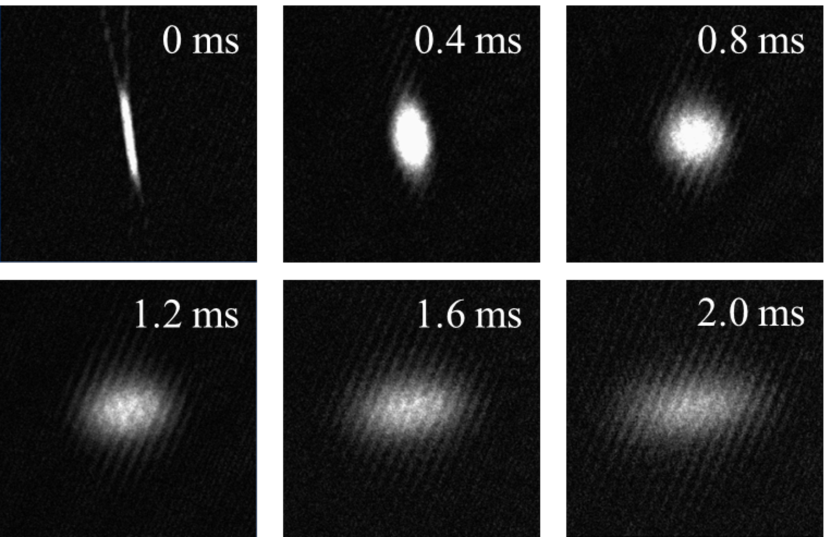
Figure 1: Absorption images of the strongly interacting Fermi gas with $B$ = 831 G at several time instances (indicated at top right of each image) after released from an anisotropic potential trap of aspect ratio of $\beta$ = 1/11.4 (crossing angle 10^∘). The field of view of each image is 0.94 mm $\times$ 0.94 mm.

We have also build a second version of ODT with the laser beam crossing angle changed to $35^{\circ}$, so that the aspect ratio of trapped atom gas is reduced to $\beta$ = 1/3.17. The prepared Fermi gas system has a total atom number $\sim 4.8\times 10^{5}$ and a degeneracy parameter $T/T_{F}$ = 0.68. The expansion experiment is repeated.

III Data Analysis

As described in Appendix C, the $z$ and $x$ projections of the absorption images are fitted with Gaussian function to extract the axial ($\sigma_{z}$) and transverse ($\sigma_{x}$) root-mean-square (RMS) size of the expanding Fermi gas, respectively. Figure 2(a) shows $\sigma_{z}$ and $\sigma_{x}$ as functions of the expansion time for $B$ = 831 G. Jitters in the data points reflect the size of statistical uncertainties, which becomes relatively large at long expansion time because of lower signal-to-noise ratio. The expansion in the axial direction is slow while it is rapid in the transverse (radial) direction; this causes the reversion of the aspect ratio. For comparison, the result with $B$ = 527 G is shown in Fig. 2(b) where the interaction vanishes and the expansion is ballistic; the aspect ratio does not reverse. Note that the measured axial size of the gas decreases initially because of absorption saturation; those axial data points are not used in subsequent analysis.

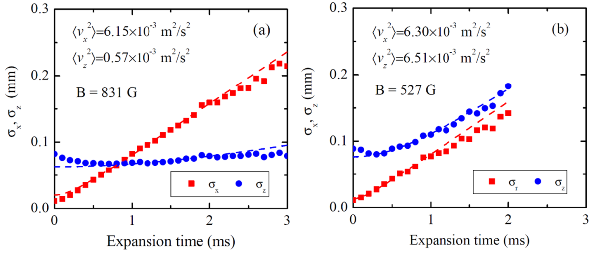
Figure 2: The RMS size of the cold-atom gas in the $z$ (axial) and $x$ (transverse) directions as functions of the expansion time. The external magnetic fields are $B$ = 831 G (a) and 527 G (b). The curves in (a) and (b) are fits to Eq.(1) within the range 1.0 – 2.0 ms and 0.3 – 1.0 ms, respectively; fitting parameters are written on the plots.

The anisotropic expansion is caused by redistribution of momentum among particles. It happens at the initial stage of expansion when interactions are strong. When the gas becomes dilute and interactions become negligible, the atoms stream freely. The late-time expansion of the cold gas cloud is treated as ballistic and can be described by [22, 23],

$$\sigma_{i}(t)^{2}=\sigma_{i}(0)^{2}+\left\langle\textit{v}_{i}^{2}\right\rangle\textit{t}^{2}\,,$$ (1)

where $i=x,y,z$ are cartesian components. Practically, free streaming starts to set in when the mean free path $\lambda=\left(\left\langle n\left(t\right)\right\rangle\sigma_{s}\right))^{-1}$ becomes larger than the average size of the expanding gas [24, 25], where $\left\langle n\left(t\right)\right\rangle$ is the mean atom density at expansion time $t$, and $\sigma_{s}$ is the s-wave scattering cross-section. At small $B$, this happens early, while for $B$ close to the Feshbach resonance point, it happens late. For $B$ = 831 G the time is found to be 0.8 ms, which is safely beyond the region of absorption saturation aforementioned. On the other hand, at long expansion time (after $\sim 2$ ms) the signal-to-noise ratio of the absorption image becomes too poor to yield a reliable RMS size. We therefore fit the 831 G data to Eq. (1) within expansion time 1.0 – 2.0 ms. The fitted $\left\langle v_{i}^{2}\right\rangle$ values along $z$ and $x$ directions are written on the plots. For $B$ = 831 G, $\left\langle v_{x}^{2}\right\rangle$ is significantly larger than $\left\langle v_{z}^{2}\right\rangle$, indicating stronger expansion in the $x$ direction than in the $z$ direction, a result of strong interactions among the atoms. Similarly, we fit the 527 G data within 0.3 – 1.0 ms. The fitted $\left\langle v_{x}^{2}\right\rangle$ and $\left\langle v_{z}^{2}\right\rangle$ values are comparable, indicating an isotropic and unchanged momentum distribution during the whole ballistic expansion process.

Results and Discussions

The momentum anisotropy of the expanding gas can be evaluated by the $v_{2}$ parameter [7],

$$\textit{v}_{2}=\frac{\left\langle v_{x}^{2}\right\rangle-\left\langle v_{z}^{2}\right\rangle}{\left\langle v_{x}^{2}\right\rangle+\left\langle v_{z}^{2}\right\rangle}\,.$$ (2)

The $v_{2}$ for $B$ = 527 G is practically zero, whereas that for 831 G is large. The interaction strength can be varied by tuning the magnetic field $B$. Figure 3 shows the $v_{2}$ parameter (red spheres) of the expanding Fermi gas as a function of the magnetic field $B$, which tunes the interaction strength. After an initial slow rise, the $v_{2}$ parameter increases rapidly with $B$ (hence the interaction strength) and apparently saturates around the Feshbach resonant value. The saturation $v_{2}$ value is large, well above 0.5.

Besides the interaction strength, the $v_{2}$ parameter also depends on the magnitude of the initial spatial anisotropy of the trapped Fermi gas. The experiment is repeated with crossing angle $35^{\circ}$, and the resultant $v_{2}$ is shown in Fig. 3 as the blue triangles. The $v_{2}$ parameter is found to be smaller than those obtained with the $10^{\circ}$ cross angle. The initial spatial anisotropy of the Fermi gas can be characterized by the eccentricity, $\varepsilon_{2}\equiv(1-\beta^{2})$/$(1+\beta^{2})$. The eccentricities of the two Fermi gases are $\varepsilon_{2}$ = 0.98 and 0.82, respectively. The observed $v_{2}$ difference is due, in part, to the difference in $\varepsilon_{2}$; one thus often divides $v_{2}$ by $\varepsilon_{2}$ when presenting data because the initial-state $\varepsilon_{2}$ is the root reason for the final-state $v_{2}$. The other part that causes a difference in $v_{2}$ is the interaction strengths of the gases that are slightly different between the two cross angles.

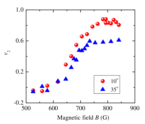
Figure 3: The $v_{2}$ parameter as a function of the magnetic field $B$. The expanding cold-atom gases are released from two ODT potential traps of differing shapes, one with beam cross angle of $10^{\circ}$ (red spheres) and the other with $35^{\circ}$ (blue triangles).

The amount of interaction can be quantified by the average number of collisions ($n$) an atom of the Fermi gas encounters during expansion. We term it opacity. For a particle traversing in a medium of uniform density $\rho$ over distance $L$ with interaction cross-section $\sigma$, it is simply $n=\rho\sigma L$. For our trapped atom gas, the opacity can be estimated by

$$\textit{n}=\frac{\sigma_{s}}{4\pi}\oint{\rho_{0}\exp\left[-\left(\frac{r^{2}\sin\theta^{2}}{2\sigma_{x}^{2}}+\frac{r^{2}\cos\theta^{2}}{2\sigma_{z}^{2}}\right)\right]\sin\theta drd\theta d\phi}\,,$$ (3)

corresponding to the average number of collisions a test atom encounters traversing out from the center of the trapped gas cloud. Here, $\rho_{0}=\frac{N}{(2\pi)^{3/2}\sigma_{x}^{2}\sigma_{z}}$ is the center density of the cold cloud of single spin. For initial RMS radii of $\sigma_{z}$ and $\sigma_{x}$ (and $\beta=\sigma_{x}/\sigma_{z}$), the integration gives $n=\frac{N\sigma_{s}}{4\pi\sigma_{x}\sigma_{z}}\frac{\arctan(\sqrt{1-\beta^{2}}/\beta)}{\sqrt{1-\beta^{2}}}$. Figure 4(a) shows $v_{2}$ (now divided by $\varepsilon_{2}$) as a function of $n$. The $v_{2}/\varepsilon_{2}$ versus $n$ data points appear to fall onto a common curve. Note that the $n$ values differ somewhat between the two cases because the initial geometries are slightly different between the two cross angles; the smaller $v_{2}$ for the $35^{\circ}$ cross angle is a combined effect of the smaller values of both $\varepsilon_{2}$ and $n$.

As mentioned in the introduction, strong elliptic flow has been observed in heavy-ion collisions. While the cold-atom gas is three-dimensional, the heavy-ion collision system is effectively two-dimensional because the longitudinal beam direction is approximately Lorentz boost invariant. The fireball created in heavy-ion collisions can be assumed to equilibrate at the typical strong interaction proper time $\tau\sim 1$ fm/$c$ with a longitudinal extent of $c\tau\sim 1$ fm, where $c$ is the velocity of light in vacuum. The initial Bjorken density [26] can be estimated by $\frac{dN_{ch}/dy}{S~{}c\tau}$ where $dN_{ch}/dy$ is the speudorapidity density of particle multiplicity and $S$ is the transverse overlap area of the two colliding nuclei. Again, taking a test particle flying out from the center of the fireball, the opacity can be estimated as $n=\frac{\sigma}{c\tau}\frac{dN_{ch}/dy}{\sqrt{\pi S}}$, where $\sigma$ = 3 mb is the parton-parton interaction cross-section. Here we have assumed isentropic evolution with entropy conservation, so one gluon turns into one final-state pion. Figure 4(b) shows the $v_{2}/\varepsilon_{2}$ as a function of $n$ in gold-gold (Au+Au) collisions over a wide range of collision energy and impact parameter [27, 28, 29, 30]. All the data points collapse onto a common curve similar to the cold-atom gas experiment. However, while the opacities are comparable, the magnitude of $v_{2}/\varepsilon_{2}$ is larger in cold-atom gas than that in heavy-ion collisions.

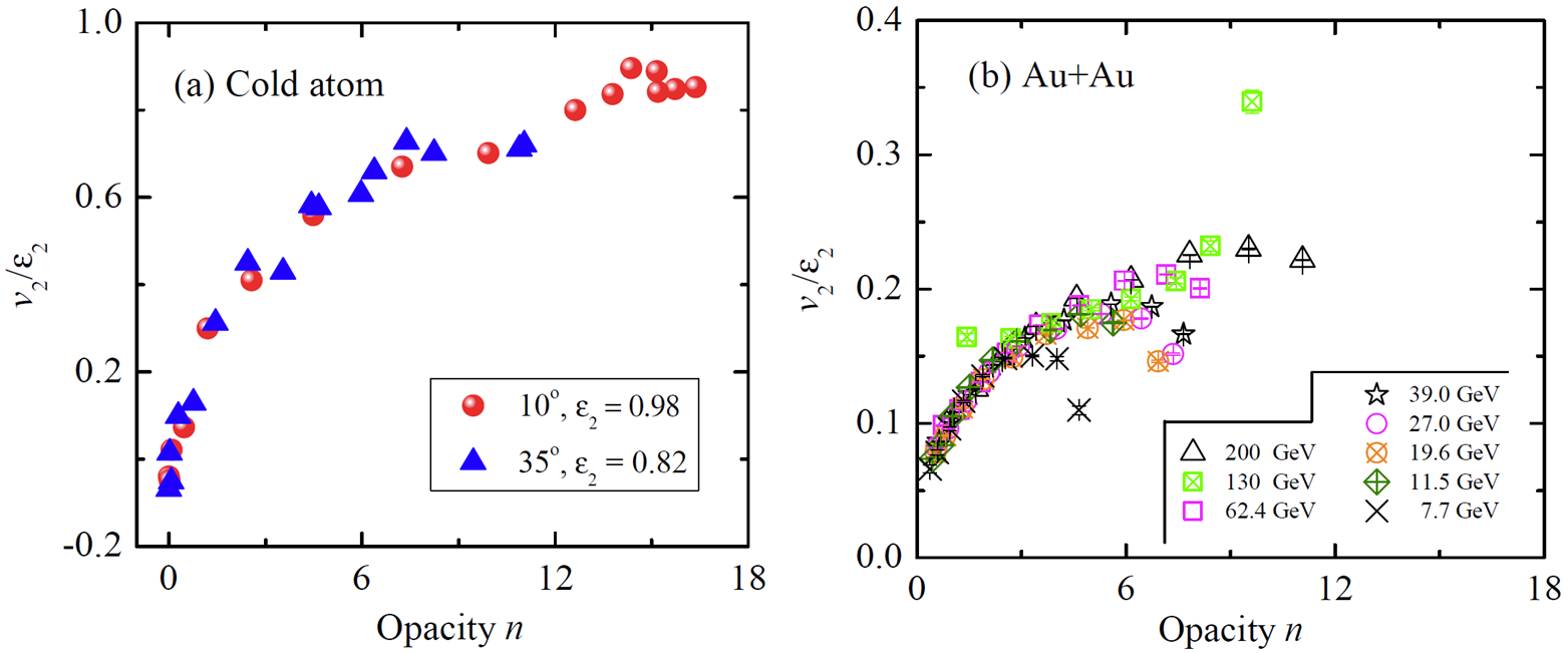
Figure 4: The eccentricity normalized $v_{2}/\varepsilon_{2}$ as a function of opacity ($n$) in cold-atom gas (a) and relativistic heavy-ion collisions (b). For the origin of heavy-ion data, please refer to Appendix G

.

There are at least two important differences between the observed $v_{2}$ from our cold atom experiment and the heavy-ion data. The first is technical: in heavy-ion experiment, the momentum is relativistic and measured particle by particle, and the $v_{2}$ parameter is averaged over all detected particles as $v_{2}=\left\langle\cos 2\phi\right\rangle=\left\langle\frac{p_{x}^{2}-p_{y}^{2}}{p_{x}^{2}+p_{y}^{2}}\right\rangle$, where $p_{x}$ and $p_{y}$ are the particle momentum components on the transverse $x$-$y$ plane [31]; in cold-atom systems which are non-relativistic, the average squared velocities are extracted from the two-dimensional density distributions obtained through absorption imaging, and the $v_{2}$ parameter is calculated by Eq.(2). To use the same definition as for cold atoms, the heavy-ion $v_{2}$ should be weighted by $p_{T}^{2}\equiv p_{x}^{2}+p_{y}^{2}$. Since $v_{2}$ is approximately proportional to transverse momentum $p_{T}$ in heavy-ion collisions, $v_{2}\propto p_{T}$ [31], and the $p_{T}$ distributions are typically exponential, $dN\propto p_{T}e^{-bp_{T}}dp_{T}$ where $b$ is a parameter related to the effective temperature [32], the $p_{T}^{2}$ weighting would amount to a factor of 2 difference: $\frac{\int p_{T}^{2}v_{2}dN}{\int p_{T}^{2}dN}$/$\frac{\int v_{2}dN}{\int dN}=2$. In other words, the $v_{2}$ in heavy-ion collisions would be a factor of 2 larger if it is calculated in the same way as in cold-atom experiment. The other difference is physical, namely non-linearity correction. The $\varepsilon_{2}$ of our cold-atom gases is close to the maximum of unity, whereas that in heavy-ion collisions is relatively small. According to hydrodynamic calculations of heavy-ion collisions [33], the effect of non-linearity for close to unity $\varepsilon_{2}$ can be as large as 50%. The linear and cubic responses are shown [33] to be approximately independent of centrality (or opacity). In other words, one should plot $v_{2}/\left[\varepsilon_{2}(1+\varepsilon_{2}^{2}/2)\right]$ in order to put systems of vastly different $\varepsilon_{2}$ onto the same footing. Such a plot is shown in Fig. 5. The cold-atom data and the heavy-ion data appear now to follow a similar trend. Ideally, one would want to make the eccentricity of the potential trap comparable to those in heavy-ion collisions by increasing the cross angle. However, this is not possible because of the space limitations around our experimental chamber. Note, for the two cold-atom gases with different $\varepsilon_{2}$, the nonlinearity corrections are similar, differing by only 10%. As such, the cold-atom gases appear consistent with each other even without nonlinearity corrections as in Fig. 4(a).

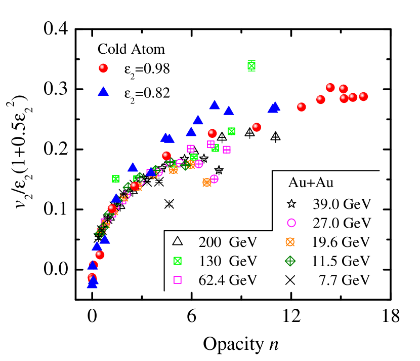
Figure 5: The $v_{2}/\left[\varepsilon_{2}(1+\varepsilon_{2}^{2}/2)\right]$ as functions of opacity ($n$). The cold-atom $v_{2}$ is first divided by 2 because of the different means to measure the $v_{2}$ from that in heavy-ion collisions (see text).

The similar trend shown in Fig. 5 suggests that the expansion dynamics is universal in interacting systems, from weak to strong. This is remarkable considering the vast differences between the two systems — the density of the QGP is $\sim 10^{39}$ cm^-3 [34] and that of a typical cold-atom gas is $\sim 10^{12}$ cm^-3 (about 7 orders thinner than air); the temperature of the QGP is $\sim 10^{12}$ K and that of a cold-atom gas is $\sim 10^{-6}$ K; the physics governing the QGP is the strong interaction of quantum chromodynamics (QCD) and that governing cold-atom gases is electromagnetic interaction of quantum electrodynamics (QED).

The universal trend exhibits two distinct regions: a sharp rise at small $n$ up to $n\approx 2$ and a flattening increase at larger $n$. This may indicate two phases with a phase transition at $n\approx 2$: a gas phase at small $n$ with minimal interactions where the anisotropy is primarily generated by the escape mechanism [11], and a liquid phase at large $n$ where the system is strongly interacting, asymptotically approaching hydrodynamics [6, 17]. It suggests that 1-2 interactions per constituent may be sufficient for a system to reach equilibrium.

Strongly interacting systems are common in nature, e.g. black holes [35], neutron stars [36], strongly coupled Bose fluid [37], superfluid liquid helium [38], and other condensed matter [39] and quantum systems [40], in addition to the QGP and cold-atom Fermi gas. Studies of quantum cold-atom gases, with their advantages of tunable interactions and variable geometries, may shed lights on non-perturbative many-body interactions in a variety of disciplines in the future [41, 42].

IV Summary

To summarize, we have carried out a cold-atom experiment with two trap geometries to systematically study the expansion behavior as a function of the interaction strength, tuned by an external magnetic field. The interaction strength is characterized by the opacity variable $n$. It is found that the anisotropy builds up quickly at small $n<2$, without the need of utterly strong interactions. The anisotropy is found to increase with interaction strength, more slowly at larger $n$. A universal behavior is quantitatively observed between the vastly different systems of cold-atom gases and heavy-ion collisions, where the non-linearity corrected eccentricity normalized elliptic anisotropy parameter $v_{2}$ follows the same trend in opacity $n$. This universality suggests that all interacting systems behave similarly in their expansion dynamics, over a wide range in interaction strength from weakly interacting systems to strongly interacting ones. The two apparently distinct regions in $n$ may suggest a phase transition from weakly interacting gas phase at small $n<2$ to strongly interacting liquid phase at large $n>2$. It indicates that 1-2 interactions per constituent may be sufficient to drive a system to equilibrium.

Our cold-atom experiment emulator can be improved in a number of ways. For example, the temperature of the atom gas can be lowered to superfluid regime to study effects of phase transition on expansion dynamics; the atom density may be increased to reach higher opacity to investigate the expansion behavior at even higher interaction strength; and the geometry of the gas cloud can be varied and a triangular geometry may be manufactured to study triangular flow expansion. The cold-atom experiment can also be extended for other tests. For example, with addition of an ion trap, one may shoot an energetic ion through a cold-atom gas to study their interactions. This would be similar to the jet quenching phenomenon [43] observed in relativistic heavy-ion collisions, another evidence for the strongly interacting QGP besides the anisotropic flow. At ion speed higher than the speed of sound of the atom gas, the Mach-cone shock wave phenomenon may be studied.

Appendix A The cold Fermi gas of ⁶Li atoms

The laser source constructing the optical dipole trap (ODT) [18] is derived from the infrared emission of a fiber laser (IPG Photonics, YLR-100-1064-LP) which is centered at 1064 nm and has a maximum power of 100 W. The beam waist of the ODT laser is $\sim 40~{}\mu$m, corresponding to a calculated trap depth of $\sim 1.8$ mK at full power. The laser is split into two parts equally, which propagate on the horizontal plane with orthogonal polarizations and are finally focused and intersected at the focal points with a crossing angle $\theta$. The crossed beams produce an anisotropic trapping potential, which can be described by a three-dimensional harmonic oscillator, $U=\frac{1}{2}m(\omega_{x}^{2}x^{2}+\omega_{y}^{2}y^{2}+\omega_{z}^{2}z^{2})$, where $m$ is the mass of ⁶Li atom, and $\omega_{i}$ is the trapping frequency along $i$-direction ($i=x,y,z$) and $\omega_{x}=\omega_{y}=\omega_{r}$. The trapping frequencies are determined mainly by the potential depth $U$, the beam waist $w_{0}$, and the crossing angle $\theta$.

The ODT is loaded with a sample of cold ⁶Li atoms directly from a magneto-optical trap (MOT) [44]. After loading, the laser power is ramped down from full power to 30 W where the trap depth is $\sim 550~{}\mu$K. The atomic population in each spin state of ⁶Li atoms, $\left|1/2,\pm 1/2\right\rangle$ [45], is resolved by using the standard RAI technique at high magnetic field to be $\sim 8.2\times 10^{5}$. The population difference between the two states is less than 12%.

The temperature of the atom gas is further lowered through two-stage evaporative cooling [46, 47]. The first stage is the so-called free evaporative cooling process, during which the external magnetic field $B$ = 841 G is switched on and the laser power is maintained at 30 W for 300 ms. Then the second stage, a forced evaporative cooling process, is conducted by lowering the laser power according to an optimized ramping trajectory. The complete process of the forced evaporative cooling takes 900 ms. Finally the laser power is reduced to 1 W, corresponding to a trap depth of $\sim 50~{}\mu$K.

Properties of the prepared Fermi gases are tabulated in Table 1. The trap depth is based on theoretical calculation; $T$ is measured with TOF of ballistic expansion; $T_{F}$ is the Fermi temperature, and $N$ is the number of atoms in a single spin state. $N$ is smaller than the initial loaded population because of evaporation during the cooling processes.

Table 1: Properties of the prepared Fermi gases

Crossing-angle	Trap Depth	$N(\times 10^{5})$	$T$	$T_{F}$	$T/T_{F}$
10∘	50 $\mu$K	5.2 $\pm$0.3	4.6 $\mu$K	6.4 $\mu$K	0.72
35∘	67 $\mu$K	2.4 $\pm$ 0.3	6.4 $\mu$K	9.4 $\mu$K	0.68

Appendix B Feshbach resonance

At zero magnetic field, the $2S_{1/2}$ ground state of ⁶Li atoms splits into two hyperfine states with total angular momentum ($\hbar$/2 and 3$\hbar$/2). In an external magnetic field $B\neq 0$, they split further into six Zeeman states as shown in Fig. 6(a), labeled $\left|i\right\rangle$ (i=1,2,…,6) [45]. The ODT can trap atoms in all of these spin states. For simplicity, our confined cold atoms are prepared in the two lowest energy states $\left|1\right\rangle$ and $\left|2\right\rangle$.

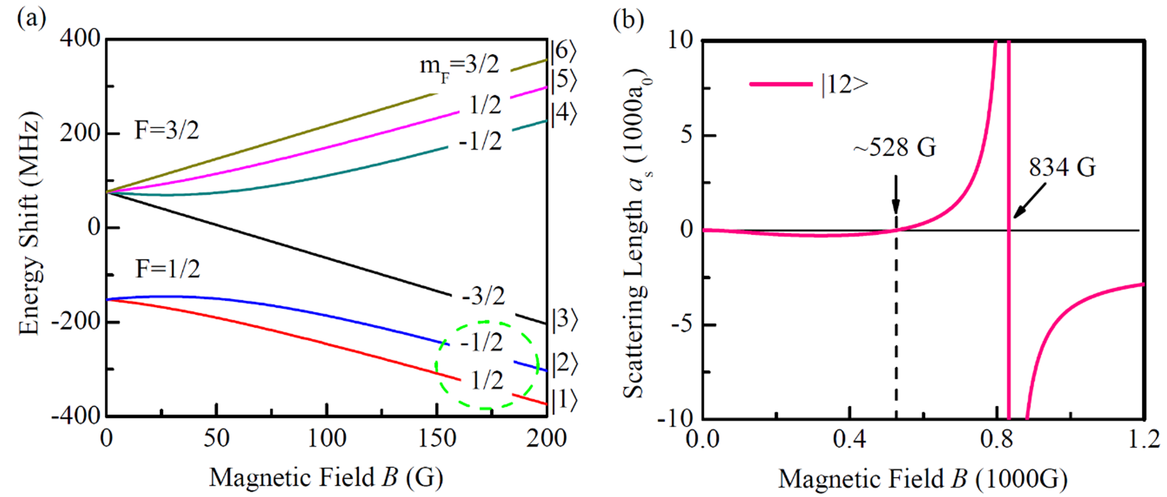
Figure 6: (a) Energy splitting of the ⁶Li $2S_{1/2}$ ground state in external magnetic field. (b) Theoretical s-wave scattering length $a_{s}$ between states $\left|1\right\rangle$ and $\left|2\right\rangle$ a function of the external magnetic field $B$; $a_{0}$ is the Bohr radius.

The interaction strength between ⁶Li atoms populated in spin states $\left|1\right\rangle$ and $\left|2\right\rangle$ can be described with a single parameter, the s-wave elastic scattering length $a_{s}$, which is controllable with the external magnetic field $B$ as shown in Fig. 6 [48]. The Feshbach resonant point between atom populated in spin states $\left|1\right\rangle$ and $\left|2\right\rangle$ is measured with Radio-Frequency (RF) Spectroscopy technique with high precision [49, 50]. In our experiment, we employ the RF spectroscopy method to determine $B$ with an accuracy of 10 mG. The s-wave scattering cross-section between atoms of different spin states is given by  [45]

$$\sigma_{s}=\frac{4\pi a_{s}^{2}}{1+k^{2}a_{s}^{2}}\,,$$ (4)

where $k=\sqrt{2mk_{B}T/\hbar^{2}}$ is the typical relative wave number of two colliding atoms. For $\left|ka_{s}\right|\gg 1$, the scattering cross-section becomes unitary limited, $\sigma_{s}=4\pi/k^{2}$; for $\left|ka_{s}\right|\ll 1$, $\sigma_{s}=4\pi a_{s}^{2}$.

As shown in Fig. 6(b), $a_{s}$ is tuned with the same magnetic field $B$ that causes the splitting of hyperfine states. When the magnetic field is tuned across 527 G, $a_{s}$ crosses zero and becomes positive. When $B$ is further approaching the Feshbach resonance point of 834 G, $a_{s}$ grows to positive infinity. For several representative magnetic field strengths of $B$ = 685, 763 and 831 G, the scattering lengths are $\sigma_{s}$ = 0.07, 0.236, and 18.6 $\mu$m, and the values of $k_{F}a_{s}$ are 0.87, 3.5, and 241, respectively. Here, $k_{F}=\sqrt{2mk_{B}T_{F}/\hbar^{2}}$ is the Fermi wave number [24].

Appendix C Resonant absorption imaging (RAI)

In our experiment, $z$-$x$ plane is horizontal with the $z$-axis lies in the axial direction and the $x$-axis in one of the radial directions, as shown Fig. 7. The external magnetic field $B$ is along the vertical direction ($y$-axis, pointing upward). The imaging beam propagates in the vertical direction and is $\sigma^{-}$ polarized (antiparallel to $B$). During imaging process, only the ODT is switched off while $B$ is kept on. After expansion time $t$, a 10 $\mu$s probe pulse is fired with light frequency finely tuned to be on resonant with the specific spin state at the given $B$. The behavior of the expanding Fermi gas can be assessed by imaging atoms populated in any one of the spin states. In our experiment, we mainly detect atoms in spin state $\left|1\right\rangle$.

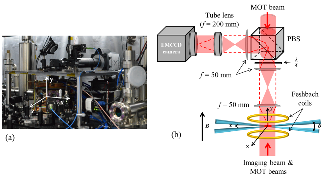
Figure 7: (a) Setup of the Fermi gas expansion experiment. (b) Schematic drawing of the detection method by absorption imaging. The magnetic field $B$ generated by a pair of Holmholtz coils (Feshbach coils) is in vertical direction ($y$-axis). Axial direction lies in $z$-axis, and the horizontal radial direction is $x$-axis. The $\theta$ refers to the crossing angle.

The center intensity of the probe light is $I_{\rm probe}=0.23$ mW/cm², corresponding to a saturation parameter $I_{\rm probe}/I_{\rm sat}\sim 0.09$, which ensures the population in the spin state is not disturbed during imaging. Here, $I_{\rm sat}=~{}2.54$ mW/cm² is the saturation intensity of D2-line transition of ⁶Li atom. The imaging system consists of two stages. The first stage is a 1:1 image-relay, which is formed with an $f$ = 50 mm lens pair. The image-relay has a numerical aperture of 0.2, corresponding to an optical resolution $\sim 2~{}\mu$m. The relayed image is magnified and projected onto the electron multiplying charge coupled device (EMCCD) camera. The pixel size of the camera sensor is 13 $\mu$m and the overall magnification of the imaging system is calibrated to be $\sim 4.15$, resulting in a spatial resolution of 3.1 $\mu$m.

Figure 8 illustrates the time sequence of the resonance absorption imaging (RAI). At the end of forced evaporative cooling, the magnetic field is ramped down from $B$ = 841 G to the set value $B$ (527–841 G) at a rate of 10 G/ms and stablized for 10 ms. The ODT laser power is then switched off and the Fermi gas is released to expand. At a given expansion time $t$, the gas is shined by a resonant light pulse of 10 $\mu$s and the absorption image $I_{\rm atom}(x,z)$ is recorded by the EMCCD camera. Two more images are recorded, each at 1500 ms later. Because the RAI technique is desctructive, the second image $I_{\rm light}(x,z)$ is recorded as a reference with no absorption. The third image $I_{\rm dark}(x,z)$ is recorded with all light blocked to serve as the dark counts of the EMCCD camera.

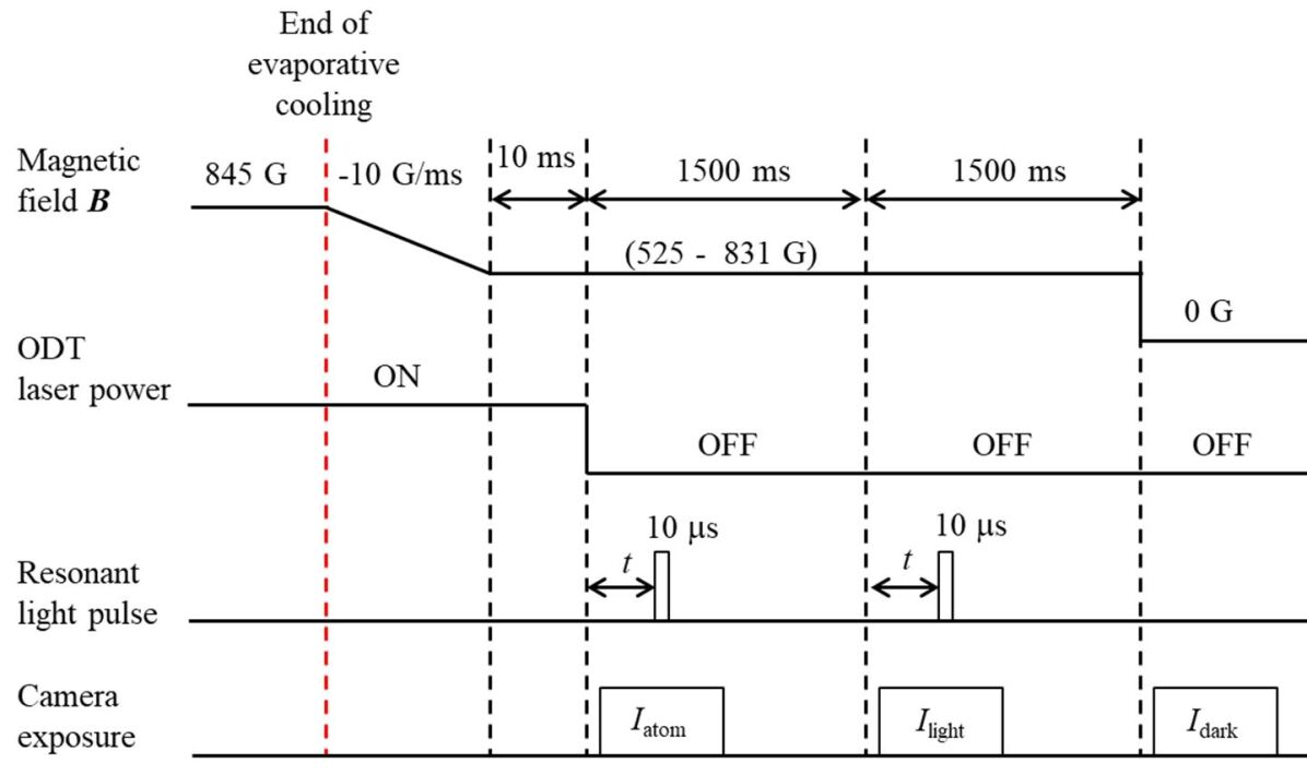
Figure 8: Time sequence of the resonance absorption imaging (RAI). Absorption imaging is conducted at non-zero magnetic field $B$ ranging from 527 G to 841 G. The ODT laser power is switched off by Acoustic Optical Modulator (AOM) in less than 1 $\mu$s.

The recorded images are digitized into two-dimensional matrices to obtain the optical density profile, $\ln\left[\frac{I_{\rm light}-I_{\rm dark}}{I_{\rm atom}-I_{\rm dark}}\right]$. The atom number per pixel in the recorded spin state is $A_{eff}/\sigma_{0}$ times the optical density, where $\sigma_{0}$ = 0.143 $\mu$m² is the resonant absorption cross-section and $A_{eff}$ = 9.81 $\mu$m² is the effective area of each pixel after considering magnification. When the optical density drops below unity, signal-to-noise ratio of the absorption image is too poor to yield reliable measurement.

Appendix D Gaussian fit

In our experiment ($T/T_{F}>0.5$), the density profile of the expanding gas can be well described by Gaussian function, $\frac{N}{(2\pi)^{3/2}\sigma_{x}\sigma_{y}\sigma_{z}}\exp\left[-\left(\frac{x^{2}}{2\sigma_{x}^{2}}+\frac{y^{2}}{2\sigma_{y}^{2}}+\frac{z^{2}}{2\sigma_{z}^{2}}\right)\right]$, in both weak and strong interaction regime, as shown in Fig. 9. This is the case described in [20].

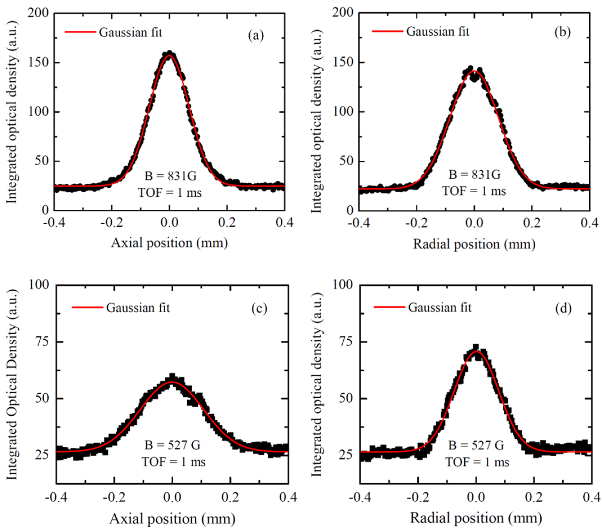
Figure 9: Axial and radial projections of the optical density profiles of the cold Fermi gases at time-of-flight (TOF) of 1 ms after their release from potential traps, for the strongly interacting case at $B$ = 831 G in (a) and (b), and for the non-interacting case at $B$ = 527 G in (c) and (d). Curves in red are Gaussian fits.

Appendix E Ballistic expansion and temperature measurement

According to [23], the scaled RMS size $b_{i}=\sigma_{i}(t)/\sigma_{i}(0)$ of ballistically expanding gas fulfills a simple differential equation, $b_{i}^{{}^{\prime\prime}}(t)-\omega_{i}^{2}/b_{i}(t)^{3}=0$, where $\omega_{i}$ is the trapping frequency along $i$-axis. This equation has an analytical solution $b_{i}(t)=\sqrt{1+(\omega_{i}t)^{2}}$ at the given initial condition, $b_{i}(0)=1$ and $b_{i}^{{}^{\prime}}(0)=0$. The radius $\sigma_{i}(t)$ is thus described by $\sigma_{i}(t)=\sigma_{i}(0)\sqrt{1+(\omega_{i}t)^{2}}$, where $\sigma_{i}(0)=(k_{B}T/m\omega_{i}^{2})^{1/2}$ is the initial in-trap RMS radius. This can be rewritten into Eq.(1) in the main text, where $\left\langle v_{i}^{2}\right\rangle=k_{B}T_{i}/m$. Equation (1) is widely used as a fitting function to extract temperature of non-interaction cold-atom systems [22, 23].

In our experiment, the confining potential is ellipsoidal with $\omega_{x}\sim\omega_{y}=\omega_{r}$ and $\beta=\omega_{z}/\omega_{r}<1$; $\beta$ determines the in-trap aspect ratio. The aspect ratio of the ballistically expanding Fermi gas is then given by  [23]

$$\frac{\sigma_{r}(t)}{\sigma_{z}(t)}=\frac{\omega_{z}}{\omega_{r}}\frac{\sqrt{1+(\omega_{r}t)^{2}}}{\sqrt{1+(\omega_{z}t)^{2}}}\,.$$ (5)

According to Eq. 5,the aspect ratio of the expanding non-interacting Fermi gas approaches unity asymptotically.

As shown in Fig. 6(b), the s-wave scattering length $a_{s}$ vanishes at $B$ = 527 G. At the end of evaporative cooling, the magnetic field is tuned to 527 G, and then the ODT laser light is switched off abruptly. The released gas expands in the homogeneous magnetic field stabilized at 527 G. Since the gas is non-interacting and follows ballistic expansion, the temperature can be extracted by fitting Eq.(1) to the size of the expanding gas from a series of TOF images, as shown in Fig. 2(b). The temperature parameters obtained from expansion data in the $x$ and $z$ directions are similar, $T_{x}=4.56~{}\mu$K and $T_{z}=4.71~{}\mu$K; the momentum distribution of the released Fermi gas is indeed isotropic. The mean value $T=(2T_{x}+T_{z})/3$ is used as the temperature $T$ in Table 1.

It should be noted that the expansion time range that can be used for temperature fitting is limited. For short expansion time, center atom density of the expanding gas is still high such that the absorption image is strongly saturated, resulting in an artificially larger RMS size extracted from Gaussian fitting. Moreover, the gas size is small at short expansion time, comparable to the spatial resolution of the imaging system. As a result the diffraction effect is significant in the radial direction ($x$-axis shown in Fig. 7), such that the fitted RMS size is also artificially larger than truth. Last, a strong loss of atoms is unavoidable when $B$ is tuned across 650 G; it is found that the atom number drops by half after $B$ is swept to 527 G. This puts a limitation on the longest applicable expansion time for imaging with high enough signal-to-noise ratios. Based on the above considerations, only data points within the range 0.3 – 1.0 ms are chosen for temperature fitting at $B$ = 527 G.

Appendix F Anisotropic expansion

In our experiment ($T>0.5~{}T_{F}$), the gas is still in normal state. When $B$ is tuned to the vicinity of the Feshbach resonance point of 834 G, an anisotropic expansion can be observed after the gas is released. This can be treated as hydrodynamic expansion where the positive s-wave scattering length is extremely large and the collisional cross-section is unitary limited [24]. Whereas the anisotropic expansion in Ref.(17) is observed at large and negative $s$-wave scattering length ($a_{s}\sim-10^{4}~{}a_{0}$) and the gas is highly degenerate ($T\sim 0.1~{}T_{F}$). Here, $a_{0}=0.53\times 10^{-10}$ m is the Bohr radius. Fig. 10 shows one-dimensional optical density profile at different expansion times. The external magnetic field is set to $B$ = 831 G, where the $s$-wave scattering length is positive ($a_{s}>$ 0) and extremely large and in the unitary limit regime. The gas expands rapidly in the radial direction (Fig. 10(b)) while remains nearly stationary in the axial direction (Fig. 10(a)) in the measured time range from 0.3 ms to 1.8 ms. The RMS sizes of the atom Fermi gas are extracted from Gaussian fits to the density profile, as shown in Fig. 2. Similar exercises are performed with other $B$ values.

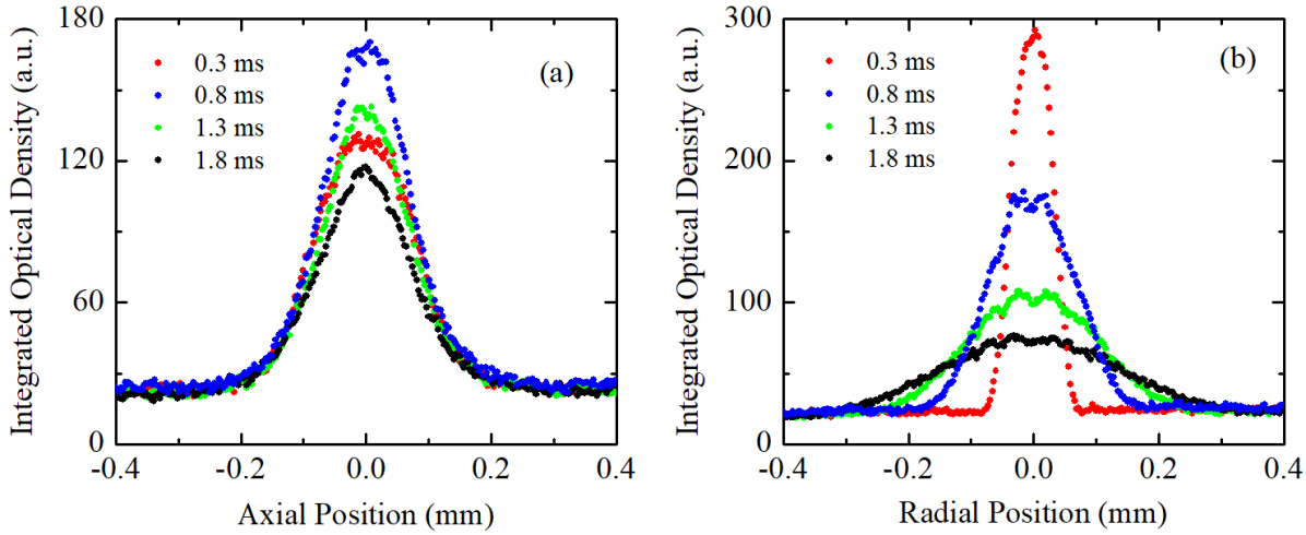
Figure 10: Integrated one-dimensional optical density profile at different expansion times, 0.3 ms (red), 0.8 ms (blue), 1.3 ms (green) and 1.8 ms (black), along axial (a) and radial direction (b). Because of absorption saturation, the axial profile of the center density at 0.3 ms is lower than that at 0.8 ms and 1.3 ms. These profiles are obtained at $B$ = 831 G.

Figure 11 shows the aspect ratio as a function of expansion time for four $B$ values. At $B$ = 527 G, the expansion is ballistic and the aspect ratio approaches unity and does not reverse. When the magnetic field is set at 685 G, a moderate reversion of the aspect ratio is observed. When the magnetic field is tuned to values around the Feshbach resonance, namely 763 and 831 G, the aspect ratio quickly exceeds unity at expansion time shorter than 1 ms. The solid curves in Fig. 11 are theoretical calculations with a set of coupled nonlinear equations as described in Ref (23) in the main text,

$$b_{i}^{{}^{\prime\prime}}(t)-\frac{\omega_{i}^{2}}{b_{i}^{3}(t)}+\frac{3}{2}\chi\omega_{i}^{2}\left(\frac{1}{b_{i}^{3}(t)}-\frac{1}{b_{i}(t)V(t)}\right)=0\,,$$ (6)

where $\chi$ quantifies the interaction strength, and $V\left(t\right)=b_{x}\left(t\right)b_{y}\left(t\right)b_{z}\left(t\right)$ is the scaled volume. For ballistic expansion at $B$ = 527 G, $\chi$ = 0; while for $B$ = 685, 763 and 831 G, $\chi$ = 0.5, 0.63 and 0.66 is chosen respectively. The high $\chi$ value represents a strong interaction strength within the gas when $B$ is tuned to the vicinity of Feshbach resonance point ($B$ = 834 G). These comparisons support the collisional hydrodynamic picture of anisotropic expansion of Fermi gas at large interaction strengths in normal state.

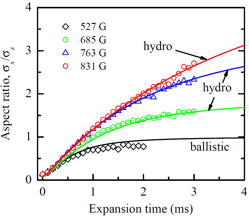
Figure 11: Aspect ratio of the expanding cold atom ⁶Li Fermi gas as a function of expansion time. The points are experimental data. The solid curves are theoretical calculations of ballistic expansion (black) and collisional hydrodynamic fits (blue, green, red) with different $\chi$ values. See text for details.

Appendix G Heavy-ion collision data

For Au+Au collisions at the nucleon-nucleon center-of-mass energy $\sqrt{s_{NN}}$ = 200 GeV and 62.4 GeV, the $v_{2}$ data are taken from Ref. [34], and the charged hadron multiplicity $dN_{ch}/dy$ and collision geometry parameters $S$ are taken from Ref. [32]. For Au+Au collisions at $\sqrt{s_{NN}}$ = 130 GeV, the $v_{2}$ data and the collision geometry parameters are taken from Ref. [28], and the multiplicity data are taken from Ref. [32]. For Au+Au collisions at $\sqrt{s_{NN}}$ = 39, 27, 19.6, 11.5, 7.7 GeV, the $v_{2}$ data and the collision geometry parameters are taken from Ref. [29], and the multiplicity data are taken from Ref. [30]. The eccentricities are calculated from nuclear collision geometry using the Glauber model [51]. The systematic uncertainties are usually large in central (small impact parameter) collisions, which is seen in the spread of the data points in Fig. 4(b) and Fig. 5. The eccentricity for the most peripheral (large impact parameter) data point at 130 GeV may also have a large uncertainty as this was one of the earliest results at RHIC [28].

References

- Shuryak [1978] E. V. Shuryak, Quark-Gluon Plasma and Hadronic Production of Leptons, Photons and Psions, Phys. Lett. B 78, 150 (1978).
- Allton et al. [2003] C. R. Allton, S. Ejiri, S. J. Hands, O. Kaczmarek, F. Karsch, E. Laermann, and C. Schmidt, The Equation of state for two flavor QCD at nonzero chemical potential, Phys. Rev. D 68, 014507 (2003), arXiv:hep-lat/0305007 .
- Adams et al. [2005] J. Adams et al. (STAR Collaboration), Experimental and theoretical challenges in the search for the quark gluon plasma: The STAR Collaboration’s critical assessment of the evidence from RHIC collisions, Nucl. Phys. A 757, 102 (2005), arXiv:nucl-ex/0501009 .
- Adcox et al. [2005] K. Adcox et al. (PHENIX Collaboration), Formation of dense partonic matter in relativistic nucleus-nucleus collisions at RHIC: Experimental evaluation by the PHENIX collaboration, Nucl. Phys. A 757, 184 (2005), arXiv:nucl-ex/0410003 .
- Roland et al. [2014] G. Roland, K. Safarik, and P. Steinberg, Heavy-ion collisions at the LHC, Prog. Part. Nucl. Phys. 77, 70 (2014).
- Gyulassy and McLerran [2005] M. Gyulassy and L. McLerran, New forms of QCD matter discovered at RHIC, Nucl. Phys. A 750, 30 (2005), arXiv:nucl-th/0405013 .
- Ollitrault [1992] J.-Y. Ollitrault, Anisotropy as a signature of transverse collective flow, Phys. Rev. D 46, 229 (1992).
- Kovtun et al. [2005] P. Kovtun, D. T. Son, and A. O. Starinets, Viscosity in strongly interacting quantum field theories from black hole physics, Phys. Rev. Lett. 94, 111601 (2005), arXiv:hep-th/0405231 .
- Dusling et al. [2016] K. Dusling, W. Li, and B. Schenke, Novel collective phenomena in high-energy proton–proton and proton–nucleus collisions, Int. J. Mod. Phys. E 25, 1630002 (2016), arXiv:1509.07939 [nucl-ex] .
- Nagle and Zajc [2018] J. L. Nagle and W. A. Zajc, Small System Collectivity in Relativistic Hadronic and Nuclear Collisions, Ann. Rev. Nucl. Part. Sci. 68, 211 (2018), arXiv:1801.03477 [nucl-ex] .
- He et al. [2016] L. He, T. Edmonds, Z.-W. Lin, F. Liu, D. Molnar, and F. Wang, Anisotropic parton escape is the dominant source of azimuthal anisotropy in transport models, Phys. Lett. B 753, 506 (2016), arXiv:1502.05572 [nucl-th] .
- Romatschke [2018] P. Romatschke, Relativistic fluid dynamics far from local equilibrium, Phys. Rev. Lett. 120, 012301 (2018).
- Kurkela et al. [2019] A. Kurkela, U. A. Wiedemann, and B. Wu, Opacity dependence of elliptic flow in kinetic theory, Eur. Phys. J. C 79, 759 (2019), arXiv:1805.04081 [hep-ph] .
- Chin et al. [2010] C. Chin, R. Grimm, P. Julienne, and E. Tiesinga, Feshbach resonances in ultracold gases, Rev. Mod. Phys. 82, 1225 (2010).
- Thomas [2010] J. E. Thomas, The nearly perfect Fermi gas, Physics Today 63, 34 (2010).
- Schäfer and Teaney [2009] T. Schäfer and D. Teaney, Nearly Perfect Fluidity: From Cold Atomic Gases to Hot Quark Gluon Plasmas, Rept. Prog. Phys. 72, 126001 (2009), arXiv:0904.3107 [hep-ph] .
- O’Hara et al. [2002] K. M. O’Hara, S. L. Hemmer, M. E. Gehm, S. R. Granade, and J. E. Thomas, Observation of a strongly interacting degenerate fermi gas of atoms, Science 298, 2179 (2002).
- Grimm et al. [2000] R. Grimm, M. Weidemüller, and Y. B. Ovchinnikov, Optical dipole traps for neutral atoms (Academic Press, 2000) pp. 95–170.
- Anderson et al. [1995] M. H. Anderson, J. R. Ensher, M. R. Matthews, C. E. Wieman, and E. A. Cornell, Observation of Bose-Einstein Condensation in a Dilute Atomic Vapor, Science 269, 198 (1995).
- Butts and Rokhsar [1997] D. A. Butts and D. S. Rokhsar, Trapped Fermi gases, Phys. Rev. A 55, 4346 (1997).
- DeMarco and Jin [1998] B. DeMarco and D. S. Jin, Exploring a quantum degenerate gas of fermionic atoms, Phys. Rev. A 58, R4267 (1998).
- Weiss et al. [1989] D. S. Weiss, E. Riis, Y. Shevy, P. J. Ungar, and S. Chu, Optical molasses and multilevel atoms: experiment, J. Opt. Soc. Am. B 6, 2072 (1989).
- Menotti et al. [2002] C. Menotti, P. Pedri, and S. Stringari, Expansion of an Interacting Fermi Gas, Phys. Rev. Lett. 89, 250402 (2002).
- Giorgini et al. [2008] S. Giorgini, L. P. Pitaevskii, and S. Stringari, Theory of ultracold atomic Fermi gases, Rev. Mod. Phys. 80, 1215 (2008).
- Bourdel et al. [2003] T. Bourdel, J. Cubizolles, L. Khaykovich, K. M. F. Magalhães, S. J. J. M. F. Kokkelmans, G. V. Shlyapnikov, and C. Salomon, Measurement of the Interaction Energy near a Feshbach Resonance in a 6Li Fermi Gas, Phys. Rev. Lett. 91, 020402 (2003).
- Bjorken [1983] J. D. Bjorken, Highly relativistic nucleus-nucleus collisions: The central rapidity region, Phys. Rev. D 27, 140 (1983).
- Agakishiev et al. [2012] G. Agakishiev et al. (STAR Collaboration), Energy and system-size dependence of two- and four-particle measurements in heavy-ion collisions at and 200 GeV and their implications on flow fluctuations and nonflow, Phys. Rev. C 86, 014904 (2012).
- Adler et al. [2002] C. Adler et al. (STAR Collaboration), Elliptic flow from two- and four-particle correlations in AuAu collisions at GeV, Phys. Rev. C 66, 034904 (2002).
- Adamczyk et al. [2012] L. Adamczyk et al. (STAR Collaboration), Inclusive charged hadron elliptic flow in AuAu collisions at –39 GeV, Phys. Rev. C 86, 054908 (2012).
- Adamczyk et al. [2017] L. Adamczyk et al. (STAR Collaboration), Bulk properties of the medium produced in relativistic heavy-ion collisions from the beam energy scan program, Phys. Rev. C 96, 044904 (2017).
- Poskanzer and Voloshin [1998] A. M. Poskanzer and S. A. Voloshin, Methods for analyzing anisotropic flow in relativistic nuclear collisions, Phys. Rev. C 58, 1671 (1998).
- Abelev et al. [2009] B. I. Abelev et al. (STAR Collaboration), Systematic measurements of identified particle spectra in , , and AuAu collisions at the star detector, Phys. Rev. C 79, 034909 (2009).
- Noronha-Hostler et al. [2016] J. Noronha-Hostler, L. Yan, F. G. Gardim, and J.-Y. Ollitrault, Linear and cubic response to the initial eccentricity in heavy-ion collisions, Phys. Rev. C 93, 014909 (2016).
- Adams et al. [2004] J. Adams et al. (STAR Collaboration), Identified particle distributions in and AuAu collisions at GeV, Phys. Rev. Lett. 92, 112301 (2004).
- Hawking [1975] S. W. Hawking, Particle Creation by Black Holes, Commun. Math. Phys. 43, 199 (1975).
- Hewish et al. [1968] A. Hewish, S. J. Bell, J. D. H. Pilkington, P. F. Scott, and R. A. Collins, Observation of a rapidly pulsating radio source, Nature 217, 709 (1968).
- LeClair [2011] A. LeClair, On the viscosity to entropy density ratio for unitary bose and fermi gases, New J. Phys. 13, 055015 (2011).
- Penrose and Onsager [1956] O. Penrose and L. Onsager, Bose-Einstein Condensation and Liquid Helium, Phys. Rev. 104, 576 (1956).
- Bloch et al. [2008] I. Bloch, J. Dalibard, and W. Zwerger, Many-body physics with ultracold gases, Rev. Mod. Phys. 80, 885 (2008), arXiv:0704.3011 [cond-mat.other] .
- Georgescu et al. [2014] I. M. Georgescu, S. Ashhab, and F. Nori, Quantum simulation, Rev. Mod. Phys. 86, 153 (2014).
- Zinner and Jensen [2013] N. T. Zinner and A. S. Jensen, Comparing and contrasting nuclei and cold atomic gases, J. Phys. G 40, 053101 (2013).
- Levinsen et al. [2017] J. Levinsen, P. Massignan, S. Endo, and M. M. Parish, Universality of the unitary fermi gas: a few-body perspective, Journal of Physics B: Atomic, Molecular and Optical Physics 50, 072001 (2017).
- Wang and Gyulassy [1992] X.-N. Wang and M. Gyulassy, Gluon shadowing and jet quenching in collisions at GeV, Phys. Rev. Lett. 68, 1480 (1992).
- Lindquist et al. [1992] K. Lindquist, M. Stephens, and C. Wieman, Experimental and theoretical study of the vapor-cell zeeman optical trap, Phys. Rev. A 46, 4082 (1992).
- O’Hara et al. [2000] K. M. O’Hara, M. E. Gehm, S. R. Granade, S. Bali, and J. E. Thomas, Stable, Strongly Attractive, Two-State Mixture of Lithium Fermions in an Optical Trap, Phys. Rev. Lett. 85, 2092 (2000).
- Granade et al. [2002] S. R. Granade, M. E. Gehm, K. M. O’Hara, and J. E. Thomas, All-Optical Production of a Degenerate Fermi Gas, Phys. Rev. Lett. 88, 120405 (2002).
- Barrett et al. [2001] M. D. Barrett, J. A. Sauer, and M. S. Chapman, All-Optical Formation of an Atomic Bose-Einstein Condensate, Phys. Rev. Lett. 87, 010404 (2001).
- Jochim et al. [2002] S. Jochim, M. Bartenstein, G. Hendl, J. H. Denschlag, R. Grimm, A. Mosk, and M. Weidemüller, Magnetic Field Control of Elastic Scattering in a Cold Gas of Fermionic Lithium Atoms, Phys. Rev. Lett. 89, 273202 (2002).
- Bartenstein et al. [2005] M. Bartenstein, A. Altmeyer, S. Riedl, R. Geursen, S. Jochim, C. Chin, J. H. Denschlag, R. Grimm, A. Simoni, E. Tiesinga, C. J. Williams, and P. S. Julienne, Precise Determination of Cold Collision Parameters by Radio-Frequency Spectroscopy on Weakly Bound Molecules, Phys. Rev. Lett. 94, 103201 (2005).
- Zürn et al. [2013] G. Zürn, T. Lompe, A. N. Wenz, S. Jochim, P. S. Julienne, and J. M. Hutson, Precise Characterization of Feshbach Resonances Using Trap-Sideband-Resolved RF Spectroscopy of Weakly Bound Molecules, Phys. Rev. Lett. 110, 135301 (2013).
- Miller et al. [2007] M. L. Miller, K. Reygers, S. J. Sanders, and P. Steinberg, Glauber modeling in high energy nuclear collisions, Ann. Rev. Nucl. Part. Sci. 57, 205 (2007), arXiv:nucl-ex/0701025 .