Probabilistic tube-based control synthesis of stochastic multi-agent systems under signal temporal logic

Eleftherios E. Vlahakis1, Lars Lindemann2, Pantelis Sopasakis3 and Dimos V. Dimarogonas1 This work was supported by the Swedish Research Council (VR), the Knut & Alice Wallenberg Foundation (KAW), the Horizon Europe Grant SymAware and the ERC Consolidator Grant LEAFHOUND. 1Division of Decision and Control Systems, School of Electrical Engineering and Computer Science, KTH Royal Institute of Technology, 10044, Stockholm, Sweden. Email: {vlahakis,dimos}@kth.se. 2Thomas Lord Department of Computer Science, Viterbi School of Engineering, University of Southern California, Los Angeles, 90089, CA, USA. Email: llindema@usc.edu. 3School of Electronics, Electrical Engineering and Computer Science, Queen’s University Belfast, Northern Ireland, UK. Email: p.sopasakis@qub.ac.uk
Abstract

We consider the control design of stochastic discrete-time linear multi-agent systems (MASs) under a global signal temporal logic (STL) specification to be satisfied at a predefined probability. By decomposing the dynamics into deterministic and error components, we construct a probabilistic reachable tube (PRT) as the Cartesian product of reachable sets of the individual error systems driven by disturbances lying in confidence regions (CRs) with a fixed probability. By bounding the PRT probability with the specification probability, we tighten all state constraints induced by the STL specification by solving tractable optimization problems over segments of the PRT, and convert the underlying stochastic problem into a deterministic one. This approach reduces conservatism compared to tightening guided by the STL structure. Additionally, we propose a recursively feasible algorithm to attack the resulting problem by decomposing it into agent-level subproblems, which are solved iteratively according to a scheduling policy. We demonstrate our method on a ten-agent system, where existing approaches are impractical.

I Introduction

Multi-agent systems (MASs) can be found in many applications, such as robotics, autonomous vehicles, and cyber-physical systems. When these systems are stochastic, the formal specification of system properties can be formulated in a probabilistic setting, enabling a trade-off between quantifying uncertainty and adjusting feasibility. As the complexity in control synthesis from temporal logic under uncertainty grows with the dimensionality of the overall system, existing approaches typically focus on single-agent schemes [1] or non-stochastic systems [2, 3].

In this paper, we focus on signal temporal logic (STL) [4], as a tool to formally formulate and verify specifications for a wide range of MAS applications. STL employs predicates as atomic elements, coupled with Boolean and temporal operators, allowing precise specification of complex spatio-temporal properties in a dynamical system. In a deterministic setting, it is possible to design sound and complete control algorithms that guarantee STL satisfaction [5], based on the quantitative semantics of STL [6]. Here we consider stochastic MASs and a stochastic optimal control problem, where the goal is to satisfy a multi-agent STL specification with a predefined probability.

To address stochasticity in the STL framework, the works in [7, 8, 9] propose risk constraints over predicates while preserving Boolean and temporal operators. Probabilistic STL in [10] allows one to express uncertainty by incorporating random variables into predicates, while [11] introduces chance-constrained temporal logic for modeling uncertainty in autonomous vehicles. Similar approaches are found in [12, 13]. Top-down approaches imposing chance constraints on the entire specification are explored in [1, 14, 15]. Although important, these works focus on single-agent or low-dimensional systems and lack guidance on extending to MASs. An extension of [1] to stochastic MASs under STL has recently been presented in [16], considering, however, only a single joint task per agent and bounded distributions.

Here, we propose a two-stage approach to solve a stochastic optimal control problem for discrete-time linear MASs subject to additive stochastic perturbations and a global STL specification permitting multiple individual and joint tasks per agent. First, we decompose the multi-agent dynamics into a deterministic system and an error closed-loop stochastic system, for which we construct a probabilistic reachable tube (PRT) [17] as the Cartesian product of reachable sets of individual error systems. These are driven by stochastic disturbances within confidence regions (CRs) with a fixed probability. By assuming independence among individual disturbances, we show that the PRT probability can be controlled by the product of probabilities selected for each individual CR and a union-bound argument applied over time. Thus, by lower bounding the PRT probability by the specification probability, we can tighten all state constraints induced by the STL specification by solving tractable optimization problems over segments of the PRT. For multi-agent STL specifications, this is a less conservative alternative to tightening approaches relying on the STL structure [1, 16]. An attainable feasible solution to the resulting deterministic problem can then be used to synthesize multi-agent trajectories that satisfy the STL specification with the desired confidence level. To the best of the authors’ knowledge, this work is the first to address stochastic MASs under STL utilizing PRTs. Subsequently, to enhance scalability, we decompose the resulting deterministic problem into agent-level subproblems, which are solved iteratively according to a scheduling policy. We show that this iterative procedure is recursively feasible, ensures satisfaction of local tasks, and guarantees nondecreasing robustness for joint tasks.

The remainder of the paper is organized as follows. Preliminaries and the control problem setup are in Sec. II. The construction of PRTs, the constraint tightening and the distributed control synthesis, are in Sec. III. An illustrative numerical example is in Sec. IV, whereas concluding remarks are discussed in Sec. V.

II Problem setup

II-A Notation and Preliminaries

Notation: The sets of real numbers and nonnegative integers are ${\rm I\!R}$ and ${\rm I\!N}$, respectively. Let $N\in{\rm I\!N}$. Then, ${\rm I\!N}_{[0,N]}=\{0,1,\ldots,N\}$. The transpose of $\xi$ is $\xi^{\intercal}$. The identity matrix is $I_{n}\in{\rm I\!R}^{n\times n}$. Let $x_{1},\ldots,x_{n}$ be vectors. Then, $x=(x_{1},\ldots,x_{n})=[x_{1}^{\intercal}\;\cdots\;x_{n}^{\intercal}]^{\intercal}$. We denote by $\bm{x}(a:b)=(x(a),\ldots,x(b))$ an aggregate vector consisting of $x(t)$, $t\in{\rm I\!N}_{[a,b]}$, representing a trajectory. When it is clear from the context, we write $\bm{x}(t)$, omitting the endpoint. When $x(t)$, $t\in{\rm I\!N}_{[a,b]}$, are random vectors, $\bm{x}(a:b)=(x(a),\ldots,x(b))$ is a random process. Let $x_{i}(t)$, for $t\in{\rm I\!N}_{[0,N]}$ and $i\in{\rm I\!N}_{[1,M]}$. Then, $\bm{x}(0:N)=(x(0),\ldots,x(N))$ denotes an aggregate trajectory when $x(t)=(x_{1}(t),\ldots,x_{M}(t))$, $t\in{\rm I\!N}_{[0,N]}$. The remainder of the division of $a$ by $b$ is $\mathrm{mod}(a,b)$. A random variable (vector) $w$ following a distribution $\mathcal{D}_{w}$ is denoted as $w\sim\mathcal{D}_{w}$, the support of $\mathcal{D}_{w}$ is $\mathrm{supp}(\mathcal{D}_{w})$, the expected value of $w$ is $\mathbb{E}(w)$, and the variance (covariance matrix) of $w$ is $\mathrm{Var}(w)$ ($\mathrm{Cov}(w)$). The probability of event $Y$ is $\mathrm{Pr}\{Y\}$. The cardinality of a set $\mathcal{V}$ is $|\mathcal{V}|$. The Minkowski sum and the Pontryagin set difference of $S_{1}\subseteq{\rm I\!R}^{n}$ and $S_{2}\subseteq{\rm I\!R}^{n}$ are $S_{1}\oplus S_{2}=\{s_{1}+s_{2}\;|\;s_{1}\in S_{1},\;s_{2}\in S_{2}\}$ and $S_{1}\ominus S_{2}=\{s_{1}\in S_{1}\;|\;s_{1}+s_{2}\in S_{1},\forall s_{2}\in S_{2}\}$, respectively.

Lemma 1 (Distributivity of Minkowski sum)

Let $\mathcal{X}_{i},\mathcal{Y}_{i}$ $\subseteq{\rm I\!R}^{n_{i}}$, $i\in{\rm I\!N}_{[1,M]}$. Then, $(\mathcal{X}_{1}\times\cdots\times\mathcal{X}_{M})\oplus(\mathcal{Y}_{1}\times\cdots\times\mathcal{Y}_{M})=(\mathcal{X}_{1}\oplus\mathcal{Y}_{1})\times\cdots\times(\mathcal{X}_{M}\oplus\mathcal{Y}_{M})$.

Proof.

It holds that $(\mathcal{X}_{1}\times\ldots\times\mathcal{X}_{M})\oplus(\mathcal{Y}_{1}\times\ldots\times\mathcal{Y}_{M})=\{(x_{1},\ldots,x_{M})+(y_{1},\ldots\,y_{M})\;|\;\forall x_{i}\in\mathcal{X}_{i},\;i\in{\rm I\!N}_{[1,M]},\mathrm{and}\;\forall y_{i}\in\mathcal{Y}_{i},\;i\in{\rm I\!N}_{[1,M]}\}=\{(x_{1}+y_{1},\ldots,x_{M}+y_{M})\;|\;\forall x_{i}\in\mathcal{X}_{i},y_{i}\in\mathcal{Y}_{i},\;i\in{\rm I\!N}_{[1,M]}\}=(\mathcal{X}_{1}\oplus\mathcal{Y}_{1})\times\ldots\times(\mathcal{X}_{M}\oplus\mathcal{Y}_{M})$. ∎

We consider STL formulas with standard syntax:

$$\varphi{}\coloneqq{}\top{}\mid{}\pi{}\mid{}\lnot\phi{}\mid{}\phi_{1}\wedge\phi_{2}{}\mid{}\phi_{1}U_{[t_{1},t_{2}]}\phi_{2},$$ (1)

where $\pi:=(\mu(x)\geq 0)$ is a predicate, $\mu(x):=a^{\intercal}x+b$ is an affine predicate function, with $a\in{\rm I\!R}^{n_{x}}$, $x\in{\rm I\!R}^{n_{x}}$, and $b\in{\rm I\!R}$, and $\phi$, $\phi_{1}$, and $\phi_{2}$ are STL formulas, which are built recursively using predicates $\pi$, logical operators $\neg$ and $\wedge$, and the until temporal operator $U$, with $[t_{1},t_{2}]\equiv{\rm I\!N}_{[t_{1},t_{2}]}$. We omit $\lor$ (or), $\lozenge$ (eventually) and $\square$ (always) operators from (1) and the sequel, as these may be defined by (1), e.g., $\phi_{1}\lor\phi_{2}=\neg(\neg\phi_{1}\wedge\neg\phi_{2})$, $\lozenge_{[t_{1},t_{2}]}\phi=\top U_{[t_{1},t_{2}]}\phi$, and $\square_{[t_{1},t_{2}]}\phi=\lnot\lozenge_{[t_{1},t_{2}]}\lnot\phi$.

Let $\pi$ be a predicate and $\phi$ an STL formula. We write $\pi\in\phi$ to indicate that $\pi$ is part of the formula $\phi$. We denote by $\bm{x}(t)\models\phi$, $t\in{\rm I\!N}$, the satisfaction of $\phi$ verified over $\bm{x}(t)=(x(t),x(t+1),\ldots)$. The validity of a formula $\phi$ can be verified using Boolean semantics: $\bm{x}(t)\models\pi\Leftrightarrow\mu(x(t))\geq 0$, $\bm{x}(t)\models\lnot\phi\Leftrightarrow\lnot(\bm{x}(t)\models\phi)$, $\bm{x}(t)\models\phi_{1}\land\phi_{2}\Leftrightarrow\bm{x}(t)\models\phi_{1}\land\bm{x}(t)\models\phi_{2}$, $\bm{x}(t)\models\phi_{1}U_{[a,b]}\phi_{2}\Leftrightarrow\exists\tau\in t\oplus{\rm I\!N}_{[a,b]}$, s.t. $\bm{x}(\tau)\models\phi_{2}\land\forall\tau^{\prime}\in{\rm I\!N}_{[t,\tau]},\bm{x}(\tau^{\prime})\models\phi_{1}$.

Based on the semantics introduced above, the horizon of a formula is recursively defined as [4]: $N^{\pi}=0$, $N^{\lnot\phi}=N^{\phi}$, $N^{\phi_{1}\land\phi_{2}}=\max(N^{\phi_{1}},N^{\phi_{2}})$, $N^{\phi_{1}\;U_{[a,b]}\phi_{2}}=b+\max(N^{\phi_{1}},N^{\phi_{2}})$.

STL is endowed with robustness metrics for assessing the robust satisfaction of a formula [6]. A scalar-valued function $\rho^{\phi}:{\rm I\!R}^{n}\times\cdots\times{\rm I\!R}^{n}\to{\rm I\!R}$ of a signal indicates how robustly a signal $\bm{x}(t)$ satisfies a formula $\phi$. The robustness function is defined recursively as follows: $\rho^{\pi}(\bm{x}(t))=\mu(x(t))$, $\rho^{\lnot\phi}(\bm{x}(t))=-\rho^{\phi}(\bm{x}(t))$,
$\rho^{\phi_{1}\land\phi_{2}}(\bm{x}(t))=\min(\rho^{\phi_{1}}(\bm{x}(t)),\rho^{\phi_{2}}(\bm{x}(t)))$,
${\tiny\rho^{\phi_{1}U_{[a,b]}\phi_{2}}(\bm{x}(t))=\max_{\tau\in t\oplus{\rm I\!N}_{[a,b]}}\left(\min(Y_{1}(\tau),Y_{2}(\tau^{\prime}))\right)}$, with $Y_{1}(\tau)=\rho^{\phi_{1}}(\bm{x}(\tau))$, $Y_{2}(\tau^{\prime})=\min_{\tau^{\prime}\in{\rm I\!N}_{[t,\tau]}}\rho^{\phi_{2}}(\bm{x}(\tau^{\prime}))$, $\pi$ being a predicate, and $\phi$, $\phi_{1}$, and $\phi_{2}$ being STL formulas.

Definition 1

Let $\mathcal{G}=(\mathcal{V},\mathcal{E})$ be an undirected graph containing no self-loops, with node set $\mathcal{V}$, cardinality $M=|\mathcal{V}|$, and edge set $\mathcal{E}$. Let also $\mathcal{V}^{\prime}\subseteq\mathcal{V}$, with $|\mathcal{V}^{\prime}|>1$, and define $\mathcal{E}_{\mathcal{V}^{\prime}}\subseteq\mathcal{E}$ as the set of edges attached to nodes $\mathcal{V}^{\prime}$. Then, $\mathcal{G}^{\prime}=(\mathcal{V}^{\prime},\mathcal{E}_{\mathcal{V}^{\prime}})$ is a clique [18], i.e., a complete subgraph of $\mathcal{G}$, if $\mathcal{E}_{\mathcal{V}^{\prime}}$ contains all possible edges between nodes $\mathcal{V}^{\prime}$. The set of cliques of $\mathcal{G}$ is defined as

$\displaystyle\mathcal{K}=\{\nu\subseteq\mathcal{V}:(\nu,\mathcal{E}_{\nu})\text{ is a complete subgraph of }\mathcal{G}\}.$ (2)

Consider a graph $\mathcal{G}=(\mathcal{V},\mathcal{E})$ with clique set $\mathcal{K}$, a clique $\nu\in\mathcal{K}$, with $\nu=(i_{1},\ldots,i_{|\nu|})$, and vectors $x_{i_{j}}(t)$, $j\in{\rm I\!N}_{[1,|\nu|]}$, with $t\in{\rm I\!N}$, Then, $x_{\nu}(t)=(x_{i_{1}}(t),\ldots,x_{i_{|\nu|}}(t))$ is an aggregate vector. We denote by $\bm{x}_{\nu}(t)\models\phi_{\nu}$ the validity of an STL formula defined over the aggregate trajectory $\bm{x}_{\nu}(t)=(x_{\nu}(t),x_{\nu}(t+1),\ldots)$. If $\pi_{\nu}\in\phi_{\nu}$, $\pi_{\nu}:=(\mu_{\nu}(x_{\nu})\geq 0)$, where $\mu_{\nu}(x_{\nu})$ is an affine predicate function of $x_{\nu}$, with $x_{\nu}=(x_{i_{1}},\ldots,x_{i_{|\nu|}})$.

II-B Multi-agent system

II-B1 Dynamics

We consider $M$ agents with dynamics

$$x_{i}(t+1)=A_{i}x_{i}(t)+B_{i}u_{i}(t)+w_{i}(t),$$ (3)

where $x_{i}(t)\in\mathcal{X}_{i}\subseteq{\rm I\!R}^{n_{i}}$, $u_{i}\in\mathcal{U}_{i}\subseteq{\rm I\!R}^{m_{i}}$, and $w_{i}(t)\in\mathcal{W}_{i}\subseteq{\rm I\!R}^{n_{i}}$ are the state, input and disturbance vectors, respectively, the initial condition, $x_{i}(0)$, is known, $(A_{i},B_{i})$ is a stabilizable pair, with $A_{i}\in{\rm I\!R}^{n_{i}\times n_{i}}$, $B_{i}\in{\rm I\!R}^{n_{i}\times m_{i}}$, $i\in{\rm I\!N}_{[1,M]}$, and $t\in{\rm I\!N}$. By collecting individual state, input, and disturbance vectors, as $x(t)=(x_{1}(t),\ldots,x_{M}(t))\in\mathcal{X}\subseteq{\rm I\!R}^{n}$, $u(t)=(u_{1}(t),\ldots,u_{M}(t))\in\mathcal{U}\subseteq{\rm I\!R}^{m}$, and $w(t)=(w_{1}(t),\ldots,w_{M}(t))\in\mathcal{W}\subseteq{\rm I\!R}^{n}$, respectively, we write the dynamics of the entire MAS as

$$x(t+1)=Ax(t)+Bu(t)+w(t),$$ (4)

where $A=\operatorname{diag}(A_{1},\ldots,A_{M})$, $B=\operatorname{diag}(B_{1},\ldots,B_{M})$, and the state, input, and disturbance sets are $\mathcal{X}=\mathcal{X}_{1}\times\cdots\times\mathcal{X}_{M}$, $\mathcal{U}=\mathcal{U}_{1}\times\cdots\times\mathcal{U}_{M}$, and $\mathcal{W}=\mathcal{W}_{1}\times\cdots\times\mathcal{W}_{M}$, respectively.

II-B2 Disturbance

We assume that the uncertain sequence $\bm{w}_{i}(0)=(w_{i}(0),w_{i}(1),\ldots)$, with $i\in{\rm I\!N}_{[1,M]}$, is an independent and identically distributed random process, and that $w_{i}(t)$ is a random vector with mean $\mathbb{E}(w_{i}(t))=0$ and positive definite covariance matrix $\mathrm{Cov}(w_{i}(t))=Q_{i}$, which is known, for all $t\in{\rm I\!N}$. We also assume that $w_{i}(t)$, $i\in{\rm I\!N}_{[1,M]}$, are independent for $t\in{\rm I\!N}$. We denote by $\mathcal{D}_{w_{i}}$ the distribution of the disturbance $w_{i}(t)\in\mathcal{W}_{i}$, where $\mathcal{W}_{i}$ is its support, which may be unbounded. We also may write that $w(t)\sim\mathcal{D}_{w}$, with $\mathrm{supp}(\mathcal{D}_{w})=\mathcal{W}=\mathcal{W}_{1}\times\cdots\times\mathcal{W}_{M}$, $\mathbb{E}(w(t))=0$, $\mathrm{Cov}(w(t))=\operatorname{diag}(Q_{1},\ldots,Q_{M})=Q$.

Because the sequence $\bm{w}(0)=(w(0),w(1),\ldots,)$ is uncertain, the trajectory of the MAS (4) becomes a random process, $\bm{x}(0)=(x(0),x(1),\ldots)$, where $x(t)$, $t\in{\rm I\!N}$, are random vectors (except $x(0)=x_{0}$), each determined by the dynamics (4) and admissible input and disturbance sequences $\bm{u}(0:t-1)$ and $\bm{w}(0:t-1)$, respectively, with $t\in{\rm I\!N}_{\geq 1}$. To avoid confusion, we do not alter notation for different realizations of $\bm{x}(\cdot)$, $\bm{u}(\cdot)$, $\bm{w}(\cdot)$.

II-B3 STL specification

Let $\mathcal{V}=\{1,\ldots,M\}$ be the set collecting the indices of all agents. The MAS is subject to a conjunctive STL formula $\phi$ with syntax as in (1), where each conjunct is either a local subformula $\phi_{i}$ involving agent $i\in\mathcal{V}$, or a joint subformula $\phi_{\nu}$ involving a subset of agents $\nu\subseteq\mathcal{V}$. We call $\nu$ a clique. By collecting all cliques $\nu$ in $\mathcal{K}_{\phi}$, the global STL task is

$\displaystyle\phi=\bigwedge_{i\in\mathcal{V}}\phi_{i}\wedge\bigwedge_{\nu\in\mathcal{K}_{\phi}}\phi_{\nu}.$ (5)

The structure of $\phi$ in (5) induces an interaction graph $\mathcal{G}=(\mathcal{V},\mathcal{E})$, where $\mathcal{V}$ is the set of nodes, and $\mathcal{E}=\{(\nu_{i},\nu_{j})\mid\nu_{i},\nu_{j}\in\nu,\;i\neq j,\;\nu\in\mathcal{K}_{\phi}\}$ is the set of edges. Let $\pi\coloneqq(\mu(y)\geq 0)$ be a predicate in $\phi$, where $\mu(y)=a^{\intercal}y+b$, with $a,y\in{\rm I\!R}^{n_{y}}$ and $b\in{\rm I\!R}$. The vector $y\in{\rm I\!R}^{n_{y}}$ represents either an individual state vector, $x_{i}\in{\rm I\!R}^{n_{i}}$, $i\in{\rm I\!N}_{[1,M]}$, or an aggregate vector, $x_{\nu}\in{\rm I\!R}^{n_{\nu}}$, collecting the states of agents in the clique $\nu\in\mathcal{K}_{\phi}$. Formula $\phi$ can specify tasks between subsets of agents, by representing their entirety as a clique. For instance, let $\nu^{\prime},\nu^{\prime\prime}\subseteq\mathcal{V}$ and consider formulas $\phi^{\prime}$, $\phi^{\prime\prime}$, involving agents from $\nu^{\prime}$, $\nu^{\prime\prime}$, respectively. Then, it is possible to specify $\phi_{\nu}=\phi^{\prime}\ast\phi^{\prime\prime}$, with $\ast\in\{\wedge,\lor,U\}$, by defining the clique $\nu=\nu^{\prime}\cup\nu^{\prime\prime}$. Without loss of generality, we assume the following.

Assumption 1

Let $\pi$ be a predicate. Then, if $\pi\in\phi$, $\neg\pi\notin\phi$.

II-C Problem statement

We wish to solve the stochastic optimal control problem

$\displaystyle\operatorname*{Min.}_{\begin{subarray}{c}\bm{u}(0),\\ \bm{x}(0)\end{subarray}}\mathbb{E}\left[\sum_{i=1}^{M}\big{(}\sum_{t=0}^{N-1}(\ell_{i}(x_{i}(t),u_{i}(t)))+V_{f,i}(x_{i}(N))\big{)}\right]$ (6a)
$\displaystyle\mathrm{s.t.\leavevmode\nobreak\ }x(t+1)=Ax(t)+Bu(t)+w(t),\;t\in{\rm I\!N}_{[0,N)},$ (6b)
$\displaystyle\;\;\;\;\;\;\mathrm{Pr}\{\bm{x}(0)\models\phi\}\geq\theta,\;\mathrm{with}\;x(0)=x_{0},$ (6c)

where $\ell_{i}:{\rm I\!R}^{n_{i}}\times{\rm I\!R}^{m_{i}}\to{\rm I\!R}$ and $V_{f,i}:{\rm I\!R}^{n_{i}}\to{\rm I\!R}$ are cost functions penalizing the first $N$ elements of the trajectories $\bm{x}_{i}(0)$, $\bm{u}_{i}(0)$, and the end point $x_{i}(N)$, respectively, with $i\in{\rm I\!N}_{[1,M]}$, the multi-agent input trajectory $\bm{u}(0)$ is the optimization variable driving the trajectory $\bm{x}(0)=(x(0),\ldots,x(N))$, originating at $x_{0}$, to satisfy the formula $\phi$ with probability $\theta\in(0,1)$, as stated in (6c), and $N$ is the underlying horizon of the formula. In fact, (6) is a planning problem, where minimization is taken over sequences of control actions, rather than over control policies. Solving the problem directly is challenging due to the probabilistic constraint, the expectation operator in the cost function, and uncertain dynamics. To handle complexity, especially with large number of agents and complex $\phi$, we transform it into a deterministic problem, which subsequently, we decompose into smaller agent-level subproblems. Additionally, we make the following assumption.

Assumption 2

For $x(0)=x_{0}$ and given $\theta\in(0,1)$, Problem (6) is feasible: There exists a sequence $\bm{u}(0)$ such that the corresponding sequence of states, $\bm{x}(0)$, satisfies $\phi$ with probability at least $\theta$.

Remark 1

Setting $\theta=1$ in (6c), enforcing $\bm{x}(0)\models\phi$ $\forall\bm{w}(0)$, typically makes sense if $\mathrm{supp}(\mathcal{D}_{w})$ is bounded.

III Main results

III-A Error dynamics and construction of probabilistic tubes

Due to the linearity in (3), the state of each agent can be decomposed into a deterministic part, $z_{i}(t)$, and an error, $e_{i}(t)$, i.e., $x_{i}(t)=z_{i}(t)+e_{i}(t)$. Consider the causal control law $u_{i}(t)=K_{i}e_{i}(t)+v_{i}(t)$, where $K_{i}\in{\rm I\!R}^{m_{i}\times n_{i}}$ is a stabilizing state-feedback gain for the pair $(A_{i},B_{i})$. Then, we may write

$\displaystyle z_{i}(t+1)$ $\displaystyle=A_{i}z_{i}(t)+B_{i}v_{i}(t),$ (7a)
$\displaystyle e_{i}(t+1)$ $\displaystyle=\bar{A}_{i}e_{i}(t)+w_{i}(t),$ (7b)

where $z_{i}(0)=x_{i}(0)$, $e_{i}(0)=0$, and $\bar{A}_{i}=A_{i}+B_{i}K_{i}$. The above choice of $u_{i}(t)$ will allows us to control the size of the reachable sets of (7b), in light of the probabilistic constraint in (6c). By defining the deterministic and stochastic components of $x(t)$, as $z(t)=(z_{1}(t),\ldots,z_{M}(t))$ and $e(t)=(e_{1}(t),\ldots,e_{M}(t))$, respectively, a deterministic input $v(t)=(v_{1}(t),\ldots,v_{M}(t))$, a block-diagonal state-feedback gain $K=\operatorname{diag}(K_{1},\ldots,K_{M})\in{\rm I\!R}^{m\times n}$, and an aggregate block-diagonal closed-loop matrix $\bar{A}=\operatorname{diag}(\bar{A}_{1},\ldots,\bar{A}_{M})$, we decompose (4) into

$\displaystyle z(t+1)$ $\displaystyle=Az(t)+Bv(t),$ (8a)
$\displaystyle e(t+1)$ $\displaystyle=\bar{A}e(t)+w(t).$ (8b)

Given a particular state feedback gain $K$, the error system (8b) can be analyzed independently of (8a). As a closed-loop system driven by the random vector $w(t)$, we can predict its trajectory $\bm{e}(0)=(e(0),\ldots,e(N))$, with $e(0)=0$, by calculating its reachable sets probabilistically. Probabilistic reachable sets and tubes for system (8b) are defined next.

Definition 2

A set $E(t)\subseteq{\rm I\!R}^{n}$, $t\in{\rm I\!N}_{[0,N]}$, is called a $t$-step probabilistic reachable set ($t$-PRS) for (8b) at probability level $\hat{\theta}_{t}\in[0,1]$, if $\mathrm{Pr}\{e(t)\in E(t)\mid e(0)=0\}\geq\hat{\theta}_{t}$.

Since $e(0)=0$, it follows that $E(0)=\{0\}$. Also, it is worth noting that for a probability level $\hat{\theta}_{t}$ a $t$-PRS $E(t)$, $t\in{\rm I\!N}_{[0,N]}$, for (8b) is not unique.

Definition 3

Let $\bm{e}(0)=(e(0),\ldots,e(N))$ be a trajectory of (8b). Then, $\bm{E}\subseteq{\rm I\!R}^{n}\times\cdots\times{\rm I\!R}^{n}$ is called a probabilistic reachable tube (PRT) for (8b) at probability level $\Theta\in[0,1]$, if $\mathrm{Pr}\{\bm{e}(0)\in\bm{E}\}\geq\Theta$.

Next, we show how to obtain $t$-PRSs for (8b) at probability levels $\hat{\theta}_{t}$, $t\in{\rm I\!N}_{[0,N]}$, by identifying subsets of $\mathcal{W}$ with a degree of concentration of $\mathcal{D}_{w}$ [17].

Definition 4

Let $w\sim\mathcal{D}_{w}$, with $\mathrm{supp}(\mathcal{D}_{w})=\mathcal{W}$. We call $\mathscr{E}_{\theta}(\mathcal{D}_{w})\subseteq\mathcal{W}$ a confidence region (CR) for $w\in\mathcal{W}$ at probability level $\theta$, if $\mathrm{Pr}\{w\in\mathscr{E}_{\theta}(\mathcal{D}_{w})\}\geq\theta$.

CRs for $w_{i}(t)$, $i\in{\rm I\!N}_{[1,M]}$, can be approximated via Monte Carlo methods or computed analytically using concentration inequalities depending on the properties of $\mathcal{D}_{w}$. Here, since we only know that $\mathbb{E}(w_{i}(t))=0$ and $\mathrm{Cov}(w_{i}(t))=Q_{i}>0$, for $t\in{\rm I\!N}$ and $i\in{\rm I\!N}_{[1,M]}$, we construct ellipsoidal CRs at probability level $\theta_{i}$ as $\mathscr{E}_{\theta_{i}}(\mathcal{D}_{w_{i}})=\{w_{i}\in{\rm I\!R}^{n_{i}}\;|\;w_{i}^{\intercal}Q_{i}^{-1}w_{i}\leq n_{i}/\theta_{i}\}$, by the multivariate Chebyshev’s inequality. Next, we show how to construct a CR for the aggregate random vector $w(t)=(w_{1}(t),\ldots,w_{M}(t))$.

Lemma 2

Let $\mathscr{E}_{\theta_{i}}(\mathcal{D}_{w_{i}})$ be a CR for $w_{i}(t)\in\mathcal{W}_{i}$, $i\in{\rm I\!N}_{[1,M]}$, at probability level $\theta_{i}$, for all $t\in{\rm I\!N}$. Then, $\mathscr{E}_{\hat{\theta}}(\mathcal{D}_{w}){}\supseteq{}\mathscr{E}_{\theta_{1}}(\mathcal{D}_{w_{1}})\times\cdots\times\mathscr{E}_{\theta_{M}}(\mathcal{D}_{w_{M}})$, is a CR of $w(t)\in\mathcal{W}$ at probability level $\hat{\theta}$ for all $t\in{\rm I\!N}$, where $\hat{\theta}\geq\Pi_{i=1}^{M}\theta_{i}$.

Proof.

Without loss of generality let $M=2$. Then, $\mathrm{Pr}\{w(t)\in\mathscr{E}_{\hat{\theta}}(\mathcal{D}_{w})\}{}\geq{}\mathrm{Pr}\{(w_{1}(t)\in\mathscr{E}_{\theta_{1}}(\mathcal{D}_{w_{1}}))\wedge(w_{2}(t)\in\mathscr{E}_{\theta_{2}}(\mathcal{D}_{w_{2}}))\}{}={}\mathrm{Pr}\{w_{1}(t)\in\mathscr{E}_{\theta_{1}}(\mathcal{D}_{w_{1}})\}\mathrm{Pr}\{w_{2}(t)\in\mathscr{E}_{\theta_{2}}(\mathcal{D}_{w_{2}})\}{}\geq{}\theta_{1}\theta_{2}$, which is true due to independence of $w_{1}(t)$, $w_{2}(t)$, for all $t\in{\rm I\!N}$. ∎

Based on the CR construction of the disturbance $w(t)$, we construct $t$-PRSs at certain probability levels for the multi-agent error system (8b) as follows.

Proposition 1

Let $\mathscr{E}_{\hat{\theta}}(\mathcal{D}_{w}){}={}\mathscr{E}_{\theta_{1}}(\mathcal{D}_{w_{1}})\times\cdots\times\mathscr{E}_{\theta_{M}}(\mathcal{D}_{w_{M}})$ be a CR for $w(t)$, where $\mathscr{E}_{\theta_{i}}(\mathcal{D}_{w_{i}})$ is an ellipsoidal CR for $w_{i}(t)$ at probability level $\theta_{i}$, with $i\in{\rm I\!N}_{[1,M]}$. Then, the sets $E(t)\subseteq{\rm I\!R}^{n}$, $t\in{\rm I\!N}_{[0,N]}$, which are recursively defined as $E(t+1)=\bar{A}E(t)\oplus\mathscr{E}_{\hat{\theta}}(\mathcal{D}_{w})$, with $E(0)=\{0\}\times\cdots\times\{0\}$, are $t$-PRSs for (8b) at probability level $\hat{\theta}\geq\Pi_{i=1}^{M}\theta_{i}$, and $E(t)=E_{1}(t)\times\cdots\times E_{M}(t)$, $t\in{\rm I\!N}_{[0,N]}$, where $E_{i}(t)$ is a $t$-PRS for (7b) at probability level $\theta_{i}$, with $i\in{\rm I\!N}_{[1,M]}$.

Proof.

Since $E(0)=\{0\}\times\cdots\times\{0\}$, we may write $E(0)=E_{1}(0)\times\cdots\times E_{M}(0)$, with $E_{i}(0)=\{0\}$, $i\in{\rm I\!N}_{[1,M]}$, from which we compute $E(1){}={}\bar{A}E(0)\oplus\mathscr{E}_{\hat{\theta}}(\mathcal{D}_{w}){}={}(\operatorname{diag}(\bar{A}_{1},\ldots,\bar{A}_{M})E_{1}(0)\times\cdots\times E_{M}(0)){}\oplus{}(\mathscr{E}_{\theta_{1}}(\mathcal{D}_{w_{1}})\times\cdots\times\mathscr{E}_{\theta_{M}}(\mathcal{D}_{w_{M}})){}={}(\bar{A}_{1}E_{1}(0)\times\cdots\times\bar{A}_{M}E_{M}(0)){}\oplus{}(\mathscr{E}_{\theta_{1}}(\mathcal{D}_{w_{1}})\times\cdots\times\mathscr{E}_{\theta_{M}}(\mathcal{D}_{w_{M}}))$, which from Lemma 1 results in $E(1){}={}\bar{A}_{1}E_{1}(0){}\oplus{}\mathscr{E}_{\theta_{1}}(\mathcal{D}_{w_{1}})\times\cdots\times\bar{A}_{M}E_{M}(0){}\oplus{}\mathscr{E}_{\theta_{M}}(\mathcal{D}_{w_{M}})$, that is, $E(1)=E_{1}(1)\times\cdots\times E_{M}(1)$, with $E_{i}(1)=\bar{A}_{i}E_{i}(0)\oplus\mathscr{E}_{\theta_{i}}(\mathcal{D}_{w_{i}})$, $i\in{\rm I\!N}_{[1,M]}$. Following the recursion, one can show that $E_{i}(t+1)=\bar{A}_{i}E_{i}(t)\oplus\mathscr{E}_{\theta_{i}}(\mathcal{D}_{w_{i}})$, for $t\in{\rm I\!N}_{[0,N-1]}$, and $E(t)=E_{1}(t)\times\cdots\times E_{M}(t)$ for $t\in{\rm I\!N}_{[0,N]}$.

Let now $\mathcal{D}_{e_{i}(t)}$ be the distribution of $e_{i}(t)$, and $\mathscr{E}_{\theta_{i}}(\mathcal{D}_{e_{i}(t)})$ be a CR for $e_{i}(t)$ at probability $\theta_{i}$. Since, $\mathscr{E}_{\theta_{i}}(\mathcal{D}_{e_{i}(0)})\subseteq E_{i}(0)=\{0\}$, we have $\bar{A}_{i}\mathscr{E}_{\theta_{i}}(\mathcal{D}_{e(0)})\oplus\mathscr{E}_{\theta_{i}}(\mathcal{D}_{w_{i}})\subseteq\bar{A}_{i}E_{i}(0)\oplus\mathscr{E}_{\theta_{i}}(\mathcal{D}_{w_{i}})=E_{i}(1)$, so $\mathscr{E}_{\theta_{i}}(\mathcal{D}_{e_{i}(1)})\subseteq E_{i}(1)$, as $\mathscr{E}_{\theta_{i}}(\mathcal{D}_{e_{i}(t+1)})\subseteq\bar{A}_{i}\mathscr{E}_{\theta_{i}}(\mathcal{D}_{e_{i}(t)})\oplus\mathscr{E}_{\theta_{i}}(\mathcal{D}_{w_{i}})$ for all $t\in{\rm I\!N}$, since $\mathscr{E}_{\theta_{i}}(\mathcal{D}_{w_{i}})$ is an ellipsoidal region by [17, Cor. 4]. Inductively we show that $\mathscr{E}_{\theta_{i}}(\mathcal{D}_{e_{i}(t)})\subseteq E_{i}(t)$, $i\in{\rm I\!N}_{[1,M]}$, for all $t\in{\rm I\!N}$. The latter implies that $\mathrm{Pr}\{e_{i}(t)\in E_{i}(t)\}\geq\theta_{i}$, $i\in{\rm I\!N}_{[1,M]}$, from which we have $\mathrm{Pr}\{e(t)\in E(t)\}=\mathrm{Pr}\{(e_{1}(t)\in E_{1}(t))\wedge\cdots\wedge(e_{M}(t)\in E_{M}(t))=\mathrm{Pr}\{(e_{1}(t)\in E_{1}(t))\}\cdots\mathrm{Pr}\{(e_{M}(t)\in E_{M}(t))\}\geq\theta_{1}\theta_{2}\cdots\theta_{M}$, which follows from the independence of $E_{i}(t)$, $i\in{\rm I\!N}_{[1,M]}$, by construction, for all $t\in{\rm I\!N}$. ∎

Proposition 1 leads to the following PRT result.

Theorem 1

Let $\mathscr{E}_{\hat{\theta}}(\mathcal{D}_{w})=\mathscr{E}_{\theta_{1}}(\mathcal{D}_{w_{1}})\times\cdots\times\mathscr{E}_{\theta_{M}}(\mathcal{D}_{w_{M}})$ be a CR for $w(t)$, and define $t$-PRSs, $E(t)$, $t\in{\rm I\!N}_{[0,N]}$ for system (8b) at probability level $\hat{\theta}\geq\Pi_{i=1}^{M}\theta_{i}$, where $\theta_{i}$ is the confidence level of the region $\mathscr{E}_{\theta_{i}}(\mathcal{D}_{w_{i}})$, $i\in{\rm I\!N}_{[1,M]}$, as in Proposition 1. Then, i) $\bm{E}_{i}=E_{i}(0)\times\cdots\times E_{i}(N)$ is a PRT for (7b) at probability level $\Theta_{i}\geq 1-N(1-\theta_{i})$, where $E_{i}(t)$, $t\in{\rm I\!N}_{[0,N]}$, is a $t$-PRS for (7b) at probability level $\theta_{i}$. ii) $\bm{E}=E(0)\times\cdots\times E(N)$ is a PRT for (8b) at probability level $\Theta=\Pi_{i=1}^{M}\Theta_{i}$. iii) Let $e_{\nu}(t+1)=\bar{A}_{\nu}e_{\nu}(t)+w_{\nu}(t)$ be the aggregate system collecting individual error systems from the clique $\nu\in\mathcal{K}_{\phi}$, where $\nu=(i_{1},\ldots,i_{|\nu|})$, $e_{\nu}(t)=(e_{i_{1}}(t),\ldots,e_{i_{|\nu|}}(t))$, $w_{\nu}(t)=(w_{i_{1}}(t),\ldots,w_{i_{|\nu|}}(t))$, and $\bar{A}_{\nu}=\operatorname{diag}(\bar{A}_{i_{1}},\ldots,\bar{A}_{i_{|\nu|}})$, and let $E_{\nu}(t)=E_{i_{1}}(t)\times\cdots\times E_{i_{|\nu|}}(t)$, $t\in{\rm I\!N}_{[0,N]}$, be its $t$-PRSs, with $E_{i_{j}}(t)$, being $t$-PRS for (7b) at probability level $\theta_{i_{j}}$, with $j\in{\rm I\!N}_{[1,|\nu|]}$. Then, $\bm{E}_{\nu}=E_{\nu}(0)\times\cdots\times E_{\nu}(N)$ is a PRT at probability level $\Theta=\Pi_{j=1}^{|\nu|}\Theta_{i_{j}}$.

Proof.

i) From Proposition 1, we have $E(t)=E_{1}(t)\times\cdots\times E_{M}(t)$, where $E_{i}(t)$ is a $t$-PRS for (7b) at probability level $\theta_{i}$. Let $\bm{e}_{i}(0)=(e_{i}(0),\ldots,e_{i}(N))$ be a trajectory of (7b). Then, $\mathrm{Pr}\{\bm{e}_{i}(0)\in\bm{E}_{i}\}=\mathrm{Pr}\{(e_{i}(0)\in E_{i}(0))\wedge\cdots\wedge(e_{i}(N)\in E_{i}(N))\}=1-\mathrm{Pr}\{(e_{i}(0)\notin E_{i}(0))\lor\cdots\lor(e_{i}(N)\notin E_{i}(N))\}\geq 1-\sum_{t=0}^{N}\mathrm{Pr}\{e_{i}(t)\notin E_{i}(t)\}=1-N(1-\theta_{i})$, where we used Boole’s inequality (BI), that $E_{i}(t)$, $t\in{\rm I\!N}_{[0,N]}$, is a $t$-PRS at probability level $\theta_{i}$, and $\mathrm{Pr}(e_{i}(0)\notin E_{i}(0)\}=0$. ii) $\mathrm{Pr}\{\bm{e}(0)\in\bm{E}\}=\mathrm{Pr}\{\left((e_{1}(0)\in E_{1}(0))\wedge\cdots\wedge(e_{M}(0)\in E_{M}(0))\right)\wedge\cdots\wedge\left((e_{1}(N)\in E_{1}(N))\wedge\cdots\wedge(e_{M}(N)\in E_{M}(N))\right)\}=\mathrm{Pr}\{\left((e_{1}(0)\in E_{1}(0))\wedge\cdots\wedge(e_{1}(N)\in E_{1}(N))\right)\wedge\cdots\wedge\left((e_{M}(0)\in E_{M}(0))\wedge\cdots\wedge(e_{M}(N)\in E_{M}(N))\right)\}=\mathrm{Pr}\{(\bm{e}_{1}(0)\in\bm{E}_{1})\wedge\cdots\wedge(\bm{e}_{M}(0)\in\bm{E}_{M})\}=\mathrm{Pr}\{\bm{e}_{1}(0)\in\bm{E}_{1}\}\cdots\mathrm{Pr}\{\bm{e}_{M}(0)\in\bm{E}_{M}\}=\Pi_{i=1}^{M}\Theta_{i}$, which follows from the independence of the PRTs $\bm{E}_{i}$, $i\in{\rm I\!N}_{[1,M]}$, by construction. iii) By setting $M=|\nu|$ the result follows from Proposition 1 and item ii) herein. ∎

Remark 2

Note that our PRT construction reduces conservatism for a large number of agents, while utilizing the union-bound argument only over time. This may require conservative choices for the probability levels, $\theta_{i}$, for the CRs of $w_{i}(t)$, $i\in{\rm I\!N}_{[1,M]}$, for large horizons. To construct, e.g., a PRT for (8b) at probability level $\Theta$, one may select uniform probability levels for the CRs as $\theta_{i}\geq 1-\frac{1-\Theta^{\frac{1}{M}}}{N}$, where $\theta_{i}\to 1$ for large $N$, regardless of $\Theta$.

III-B Constraint tightening

Based on the decomposition of (4) into deterministic and stochastic components, we aim to design a trajectory for the deterministic system (8a) that satisfies an STL formula derived from $\phi$, incorporating tighter predicates. The following proposition underpins this approach.

Proposition 2

Let $\bm{x}(0)=(x(0),\ldots,x(N))$ be a trajectory of (6b), and $\bm{z}(0)=(z(0),\ldots,z(N))$ and $\bm{e}(0)=(e(0),\ldots,e(N))$ be its deterministic and stochastic components with respect to the dynamics (8a) and (8b), respectively, that is, $\bm{x}(0)=\bm{z}(0)+\bm{e}(0)$. Suppose that $\mathrm{Pr}\{\bm{e}(0)\in\bm{E}\}\geq\theta$, for some $\bm{E}=E(0)\times\cdots\times E(N)$, with $E(t)\subseteq{\rm I\!R}^{n}$, $t\in{\rm I\!N}$. If $\bm{z}(0)+\bm{e}(0)\models\phi$ for all $\bm{e}(0)\in\bm{E}$, then $\mathrm{Pr}\{\bm{x}(0)\models\phi\}\geq\theta$.

Proof.

Define events $Y_{x}:=\bm{x}(0)\models\phi$, $Y_{e}:=\bm{e}(0)\in\bm{E}$, and $Y_{e}^{\prime}:=\bm{e}(0)\notin\bm{E}$. From the law of total probability, we have $\mathrm{Pr}\{Y_{x}\}=\mathrm{Pr}\{Y_{x}|Y_{e}\}\mathrm{Pr}\{Y_{e}\}+\mathrm{Pr}\{Y_{x}|Y_{e}^{\prime}\}\mathrm{Pr}\{Y_{e}^{\prime}\}\geq\theta$, since by assumption, $\mathrm{Pr}\{Y_{x}|Y_{e}\}=1$ and $\mathrm{Pr}\{Y_{e}\}\geq\theta$, and $\mathrm{Pr}\{Y_{x}|Y_{e}^{\prime}\}\mathrm{Pr}\{Y_{e}^{\prime}\}\geq 0$. ∎

Let $\bm{E}$ be a PRT for (8b) at probability level $\theta$. Next, we construct a formula $\psi$ such that $\bm{z}(0)\models\psi$ implies $\bm{z}(0)+\bm{e}(0)\models\phi$, for all $\bm{e}(0)\in\bm{E}$, that is, $\mathrm{Pr}\{\bm{x}(0)\models\phi\}\geq\theta$, by Proposition 2. Formula $\psi$ has identical Boolean and temporal operators with $\phi$ in (5), and retains its multi-agent structure:

$\displaystyle\psi=\bigwedge_{i\in\mathcal{V}}\psi_{i}\wedge\bigwedge_{\nu\in\mathcal{K}_{\phi}}\psi_{\nu}.$ (9)

Let $\pi:=(a^{\intercal}y+b\geq 0)$ be a predicate, with $a,y\in{\rm I\!R}^{n_{y}}$, $b\in{\rm I\!R}$. We denote by $\tau(\pi)$ the tighter version of $\pi$, where $\tau(\pi)\in\psi$ if $\pi\in\phi$, and $\neg\tau(\pi)\in\psi$ if $\neg\pi\in\phi$, with

$\displaystyle\tau(\pi):=(a^{\intercal}y+b+\min_{g\in G}a^{\intercal}g\geq 0),\;\text{if\;}\tau(\pi)\in\psi,$ (10a)
$\displaystyle\tau(\pi):=(a^{\intercal}y+b+\max_{g\in G}a^{\intercal}g\geq 0),\text{if\;}\neg\tau(\pi)\in\psi.$ (10b)

Here, $G=\bigcup_{t=1}^{N}E_{i}(t)$ if $y=x_{i}(t)$, for some $i\in\mathcal{V}$, or $G=\bigcup_{t=1}^{N}E_{\nu}(t)$ if $y=x_{\nu}(t)$ for some $\nu\in\mathcal{K}_{\phi}$. Also, $a$, $b$ in (10) indicate the parameters of predicate functions associated with predicates contained in $\phi_{i}$ or $\phi_{\nu}$ (retained in $\psi_{i}$ or $\psi_{\nu}$, as per (10)), with $i\in\mathcal{V}$, $\nu\in\mathcal{K}_{\phi}$. Distinguishing tightening between (10a) or (10b) while constructing $\psi$ is possible by Assumption 1, which is not restrictive since we can always have $\pi,\neg\pi^{\prime}\in\phi$, where $\pi^{\prime}=\pi$. We also remark that the optimizations in (10) are tractable since the domain $G$ is the union of finitely many convex and compact sets by the construction of $t$-PRSs, $E_{i}(t)$, $E_{\nu}(t)$, $t\in{\rm I\!N}_{[1,N]}$, in Proposition 1 and Theorem 1. Practically, the tightening in (10) can be retrieved by solving a convex optimization by taking the convex hull of $G$, or, better, by solving $N$ convex optimization problems, one for every $E_{i}(t)$, $E_{\nu}(t)$, $t\in{\rm I\!N}_{[1,N]}$, and selecting the worst-case (minimum for (10a) and maximum for (10b)) solution among them. We are now ready to state the following result.

Theorem 2

Let $\psi$ be the STL formula resulting from $\phi$ according to (9)-(10), and assume that the deterministic problem:

$\displaystyle\operatorname*{Minim.}_{\begin{subarray}{c}\bm{v}(0),\\ \bm{z}(0)\end{subarray}}\sum_{i=1}^{M}\left(\sum_{t=0}^{N-1}(\ell_{i}(z_{i}(t),v_{i}(t)))+V_{f,i}(z_{i}(N))\right)$ (11a)
$\displaystyle\mathrm{s.t.\leavevmode\nobreak\ }z(t+1)=Az(t)+Bv(t),\;t\in{\rm I\!N}_{[0,N)},$ (11b)
$\displaystyle\;\;\;\;\;\;\bm{z}(0)\models\psi,\;\mathrm{with}\;z(0)=x_{0},$ (11c)

has a feasible solution $\bm{v}(0)=(v(0),\ldots,v(N-1))$, with $v(t)\in\mathcal{U}\ominus KE(t)$, $t\in{\rm I\!N}_{[0,N-1]}$, where $K$ is a stabilising gain for $(A,B)$ in (8b), and $E(t)=E_{1}(t)\times\cdots\times E_{M}(t)$, $E_{i}(t)$, $i\in{\rm I\!N}_{[1,M]}$, being $t$-PRS for (7b), at probability level $\theta_{i}$, such that $\Pi_{i=1}^{M}\left(1-N(1-\theta_{i})\right)\geq\theta$. Let $\bm{e}(0)=(e(0),\ldots,e(N))$ be a trajectory of (8b). Then, $\bm{u}(0)=\tilde{K}\bm{e}(0)+\bm{v}(0)$ is a feasible solution for (6), where $\tilde{K}=\operatorname{diag}(K,\ldots,K)$.

Proof.

By Theorem 1, $\bm{E}=E(0)\times\cdots\times E(N)$ is a PRT for (8b) at probability level $\Theta\geq\theta$, that is, $\mathrm{Pr}\{\bm{e}(0)\in\bm{E}\}\geq\theta$. Let $\bm{z}(0)$ be a trajectory resulting from the input trajectory $\bm{v}(0)$ starting from $z(0)=x_{0}$, satisfying (11c), that is, $\bm{z}(0)\models\psi$. By the tightening in (10), we have that for all $\pi\in\phi$, $\tau(\pi)\in\psi$, such that if $\bm{z}(0)\models\tau(\pi)$, then $\bm{z}(0)+\bm{e}(0)\models\pi$ for all $\bm{e}(0)\in\bm{E}$, and for all $\neg\pi^{\prime}\in\phi$, $\neg\tau(\pi^{\prime})\in\psi$, such that if $\bm{z}(0)\models\neg\tau(\pi^{\prime})$, then $\bm{z}(0)+\bm{e}(0)\models\neg\pi^{\prime}$ for all $\bm{e}(0)\in\bm{E}$. Since $\phi$ and $\psi$ differ only in predicates in the aforementioned manner, it follows that if $\bm{z}(0)\models\psi$, then $\bm{z}(0)+\bm{e}(0)\models\phi$ for all $\bm{e}(0)\in\bm{E}$. Since $\bm{u}(0)=\tilde{K}\bm{e}(0)+\bm{v}(0)$ is a feasible input trajectory for (4) for all $\bm{e}(0)\in\bm{E}$, the resulting state trajectory of (4), $\bm{x}(0)=\bm{z}(0)+\bm{e}(0)$, ensures that $\mathrm{Pr}\{\bm{x}(0)\models\phi\}=1$ for all $\bm{e}(0)\in\bm{E}$. Then, the result follows by Proposition 2 since $\mathrm{Pr}\{\bm{e}(0)\in\bm{E}\}\geq\theta$. ∎

Clearly, apart from the volume of $\bm{E}$, the gain $K$ affects the feasible domain of (11) too. Due to space limitations, we will present its construction in future work. By selecting $\|{}\cdot{}\|_{1}$-based costs, problem (11) can be formulated as a mixed-integer linear program (MILP) using binary encoding for STL constraints [5]. The complexity of (11), which grows with the dimension of the MAS, is addressed in the next section.

III-C Distributed control synthesis

We propose an iterative procedure that handles the complexity of (11), extending the practicality of the multi-agent framework at hand. First, we assume the following.

Assumption 3

Let the $t$-PRSs, $E(t)$, $t\in{\rm I\!N}_{[0,N]}$, for (8b), and the stabilizing gain, $K$, for the pair $(A,B)$, be as constructed in Theorem 2. Then, (11) has a feasible solution $\bm{v}(0)=(v(0),\ldots,v(N-1))$, where $v(t)\in\mathcal{U}\ominus KE(t)$, $t\in{\rm I\!N}_{[0,N-1]}$.

III-C1 Decomposition of STL formula $\psi$

For a node $i$ participating in at least one clique, i.e., $i\in\nu$, with $\nu\in\mathcal{K}_{\phi}$, we define $\mathcal{T}_{i}$ by the set of cliques containing $i$ excluding $i$, i.e.,

$$\mathcal{T}_{i}=\{\nu\setminus i:\nu\in\operatorname{cl}(i)\},$$ (12)

where $\operatorname{cl}(i)=\{\nu\in\mathcal{K}_{\phi},\;\nu\ni i\}$ is the set of cliques that contain $i$. Let $j\in\mathcal{T}_{i}$, with $j=(i_{1},\ldots,i_{|j|})$. Let a trajectory $\bm{z}_{ij}(0)=(z_{ij}(0),\ldots,z_{ij}(N))$, where $z_{ij}(t)=(z_{i_{1}}(t),\ldots,z_{i}(t),\ldots,z_{i_{|j|}}(t))$, with $t\in{\rm I\!N}_{[0,N]}$, and the order $i_{1}<\ldots<i<\ldots<i_{|j|}$ being specified by the lexicographic ordering of the node set $\mathcal{V}={\rm I\!N}_{[1,M]}$. Using (12), an equivalent formula to the tighter formula (9)-(10), $\psi$, is defined as $\hat{\psi}=\bigwedge_{i\in\mathcal{V}}\hat{\psi}_{i}$, where

$$\hat{\psi}_{i}=\psi_{i}\wedge\bigwedge_{j\in\mathcal{T}_{i}}\psi_{ij}.$$ (13)

III-C2 Iterative algorithm

For simplicity, we drop the time argument and introduce an iteration index as a superscript in the trajectory notation, e.g., $\bm{z}_{i}^{k}$ ($\bm{z}_{ij}^{k}$) indicates a trajectory $\bm{z}_{i}(0)$ ($\bm{z}_{ij}(0)$) that is retrieved at the $k$th iteration of the following procedure. To initialize the procedure, we generate initial guesses on the agents’ trajectories by solving

$\displaystyle\operatorname*{Minimize}_{\begin{subarray}{c}\bm{v}_{i}^{0},\bm{z}_{i}^{0}\end{subarray}}\sum_{t=0}^{N-1}(\ell_{i}(z_{i}^{0}(t),v_{i}^{0}(t)))+V_{f,i}(z_{i}^{0}(N))$ (14a)
$\displaystyle\mathrm{s.t.\leavevmode\nobreak\ }z_{i}^{0}(t+1)=A_{i}z_{i}^{0}(t)+B_{i}u_{i}^{0}(t),\;t\in{\rm I\!N}_{[0,N)},$ (14b)
$\displaystyle\;\;\;\;\;\;\bm{z}_{i}^{0}\models\psi_{i},\;\mathrm{with}\;z_{i}^{0}(0)=x_{0,i},$ (14c)

at $k=0$ for $i\in{\rm I\!N}_{[1,M]}$. Note that by Assum. 3, Problem (14) is guaranteed to be feasible. After performing the above initialization routine, at iteration $k\geq 1$, only a subset of agents, denoted by $\mathcal{O}_{k}{\subset}\mathcal{V}$, are allowed to update their input sequences by performing an optimization, while the remaining agents retrieve their input sequences from the previous iteration $k-1\geq 0$. Roughly, the set $\mathcal{O}_{k}\subset\mathcal{V}$ is constructed so that any combination of its elements does not belong to a clique $\nu\in\mathcal{K}_{\phi}$. Due to space limitations, we simply construct $\mathcal{O}_{k}$ as a singleton, which only affects the number of agents’ trajectories that can be optimized in parallel per iteration. For the graph $\mathcal{G}=(\mathcal{V},\mathcal{E})$, with $\mathcal{V}={\rm I\!N}_{[1,M]}$, $\mathcal{O}_{k}=\mathrm{mod}(\mathcal{O}_{k-1},M)+1$, for $k>1$, with $\mathcal{O}_{1}=1$. We refer readers to [19, Sec. V.B] for a more efficient construction of $\mathcal{O}_{k}$ enabling parallel computations at each iteration (see Sec. IV for a numerical example).

At the $k$th iteration, with $k\geq 1$, if $i\notin\mathcal{O}_{k}$, then, $\bm{z}_{i}^{k}=\bm{z}_{i}^{k-1}$ and $\bm{v}_{i}^{k}=\bm{v}_{i}^{k-1}$. Otherwise, the input sequence of the $i$th agent is updated by solving

$\displaystyle\operatorname*{Minim.}_{\begin{subarray}{c}\bm{v}_{i}^{k},\bm{z}_{i}^{k}\end{subarray}}\sum_{t=0}^{N-1}(\ell_{i}(z_{i}^{k}(t),v_{i}^{k}(t)))+V_{f,i}(z_{i}^{k}(N))-\mu_{ij_{k}}^{k}$ (15a)
$\displaystyle\mathrm{s.t.\leavevmode\nobreak\ }z_{i}^{k}(t+1)=A_{i}z_{i}^{k}(t)+B_{i}v_{i}^{k}(t),\;t\in{\rm I\!N}_{[0,N)},$ (15b)
$\displaystyle\;\;\;\;\;\;\bm{z}_{i}^{k}\models\psi_{i},\;\mathrm{with}\;z_{i}(0)=x_{0,i},$ (15c)
$\displaystyle\;\;\;\;\;\;\rho^{\psi_{ij_{k}}}(\bm{z}_{ij_{k}}^{k})\geq\mu_{ij_{k}}^{k},\;j_{k}=\operatorname*{argmin}_{j\in\mathcal{T}_{i}}\{\rho^{\psi_{ij}}(\bm{z}_{ij}^{k-1})\},$ (15d)
$\displaystyle\;\;\;\;\;\;\mu_{ij_{k}}^{k}\geq\min\left(0,\rho^{\psi_{ij_{k}}}(\bm{z}_{ij_{k}}^{k-1})\right),$ (15e)
$\displaystyle\;\;\;\;\;\;\rho^{\psi_{ij}}(\bm{z}_{ij}^{k})\geq\min\left(0,\rho^{\psi_{ij}}(\bm{z}_{ij}^{k-1})\right),\;\forall j\in\mathcal{T}_{i}\setminus j_{k},$ (15f)

where $\rho^{\psi_{ij}}(\bm{z}_{ij}^{k})$ is the robustness function of the formula $\psi_{ij}$ evaluated over the trajectory $\bm{z}_{ij}^{k}$. Agent-$i$, with $i\in\mathcal{O}_{k}$, by solving (15), retrieves an input sequence that guarantees 1) the satisfaction of the individual task $\psi_{i}$ (see constraint (15c)), 2) the improvement of the most violating (or least robust) joint task $\psi_{ij_{k}}$ (see constraints (15d)-(15e)), and 3) either improvement on or non-violation of the remaining joint tasks (see constraint (15f)). The inclusion of the $\min$ operator in the constraints (15e)-(15f) relaxes the satisfaction of joint tasks that have already been found to be satisfiable in previous iterations. This allows the algorithm to emphasize the satisfaction of joint tasks with the smallest robustness function verified on trajectories attained in previous iterations. Based on the following result, these key features are ensured to persist at each iteration. The algorithm may terminate if it exceeds a maximum number of iterations, denoted as $k_{\mathrm{max}}$ and defined by the designer. Alternatively, termination occurs when verifying the satisfiability of all joint tasks, i.e., when $\mu_{ij}^{k}\geq 0$ for all $i\in\mathcal{V}$, $j\in\mathcal{T}_{i}$, and some $k\leq k_{\mathrm{max}}$. Given that the algorithm is not required to operate online, $k_{\mathrm{max}}$ may be determined ad-hoc. The overall iterative procedure is summarized in Algorithm 1.

Theorem 3

At each iteration $k\geq 1$, the optimization problem (15) is feasible for all $i\in\mathcal{O}_{k}$.

Proof.

Let $k=1$. The lower bounds in (15d)-(15f) are defined over trajectories, $\bm{z}_{i}^{0}$, $i{\in}\mathcal{O}_{1}$, obtained by solving (14) at $k{=}0$. Thus $\bm{z}_{i}^{0}$ satisfies the constraints (15d)-(15f) for all $i{\in}\mathcal{O}_{1}\subset\mathcal{V}$. Moreover, the constraint in (15c) is satisfied by $\bm{z}_{i}^{0}$, since (14) is feasible by Assum. 3. Hence, $\bm{u}_{i}^{1}=\bm{u}_{i}^{0}$ is a feasible solution of (15) at iteration $k=1$. Now, let $k{>}1$. Similarly, the lower bounds in (15d)-(15f) are defined over trajectories, $\bm{z}_{i}^{k-1}$, obtained by the solutions $\bm{u}_{i}^{k-1}$, $i{\in}\mathcal{O}_{k}$, at iteration $k-1$. Thus, $\bm{z}_{i}^{k-1}$, $i{\in}\mathcal{O}_{k}$, satisfy the constraints (15d)-(15f). Additionally, the constraint in (15c) is satisfied by $\bm{z}_{i}^{k-1}$, $i\in\mathcal{O}_{k}$, since it is retrieved by $\bm{u}_{i}^{k-1}$, which is obtained by solving (15) or (14) at some iteration $\kappa\in{\rm I\!N}_{[0,k-1]}$. Thus, $\bm{u}_{i}^{k}{=}\bm{u}_{i}^{k-1}$ is a feasible solution of (15) at iteration $k>1$. We have shown that (15) is feasible for all $i\in\mathcal{O}_{k}$ at $k{=}1$ and any $k{>}1$, so the result follows. ∎

Algorithm 1 Iterative procedure for solving (11)
1:Compute $\mathcal{T}_{i}$ and construct $\hat{\psi}_{i}$ by (13), for $i\in{\rm I\!N}_{[1,M]}$
2:Solve (14) and store $\bm{v}_{i}^{0}$, $\bm{z}_{i}^{0}$, for $i\in{\rm I\!N}_{[1,M]}$
3:Construct $\mathcal{O}_{k}$, for $k\in{\rm I\!N}_{[1,k_{\mathrm{max}}]}$
4:for $k$ in $1:k_{\mathrm{max}}$ do
5:     if $i\in\mathcal{O}_{k}$ solve (15), store $\bm{v}_{i}^{k}$ and compute $\bm{z}_{i}^{k}$
6:     if $i\notin\mathcal{O}_{k}$ update $\bm{v}_{i}^{k}=\bm{v}_{i}^{k-1}$ and $\bm{z}_{i}^{k}=\bm{z}_{i}^{k-1}$
7:     Construct $\bm{v}(0)$ from $\bm{v}_{i}^{k}$, $\bm{z}(0)$ from $\bm{z}_{i}^{k}$, $i\in{\rm I\!N}_{[1,M]}$
8:     if $\rho^{\psi}(\bm{z}(0))\geq 0$ go to 9
9:return $\bm{v}(0)$, $\bm{z}(0)$
Remark 3

Algorithm 1 yields a minimally violating solution within a designer-defined iteration limit. If a solution is obtained before reaching the maximum iterations, it is guaranteed to be feasible for (11). By Theorem 2, a feasible solution for (6) can then be efficiently constructed.

IV Example

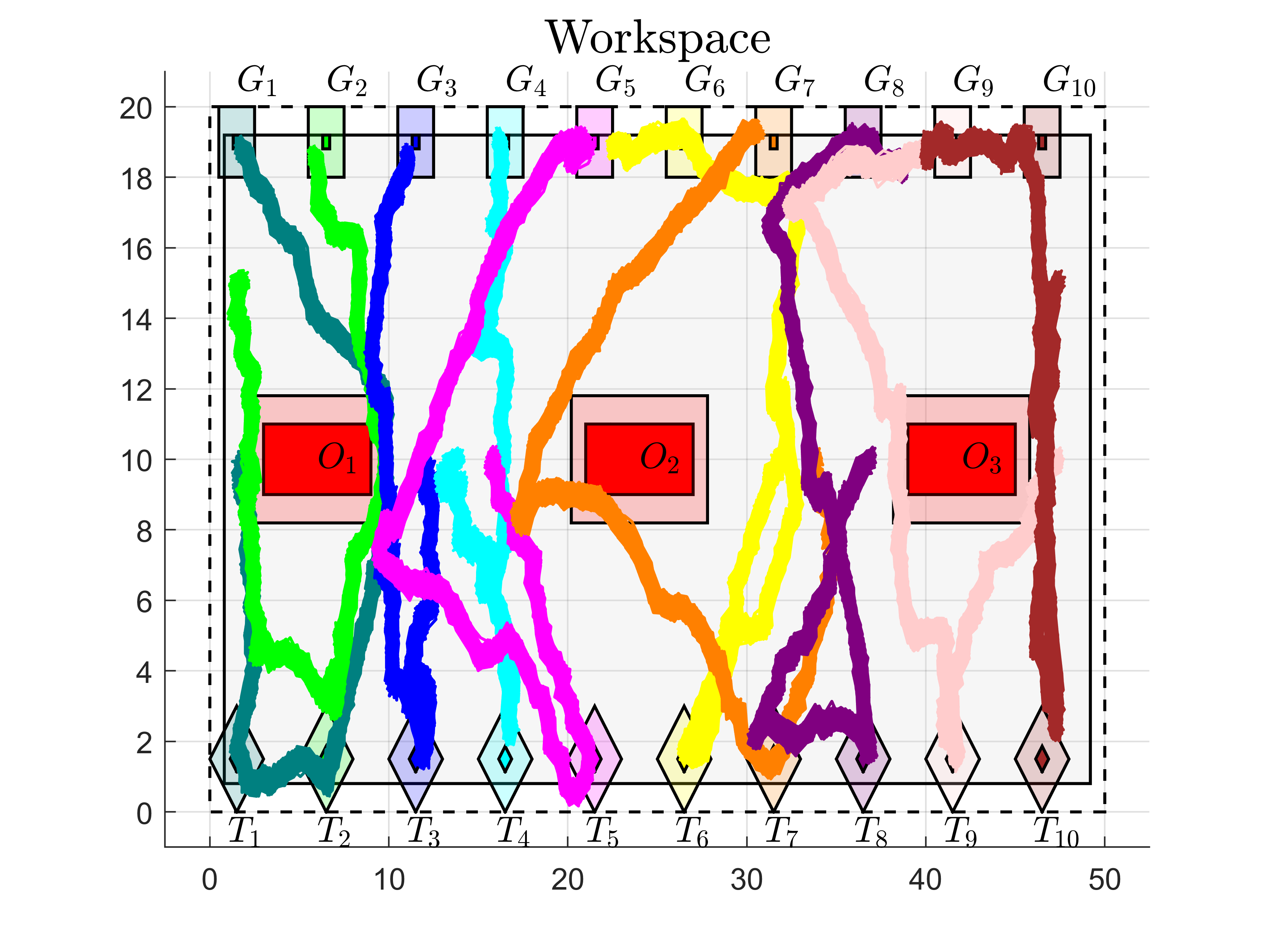
We consider a MAS of ten agents with global dynamics given by $x(t+1)=x(t)+u(t)+w(t)$, where $x(t)=(x_{1}(t),..,x_{10}(t))\in{\rm I\!R}^{20}$, $u(t)=(u_{1}(t),..,u_{10}(t))\in{\rm I\!R}^{20}$, and $w(t)=(w_{1}(t),..,w_{10}(t))\in{\rm I\!R}^{20}$. Individual states are constrained by $x_{i}(t)\in\mathcal{X}$, where $\mathcal{X}$ is the workspace of MAS, confined by the dashed border shown in Fig. 4, individual inputs are constrained by $\|u_{i}(t)\|_{\infty}\leq 0.8$, and individual disturbances, $w_{i}(t)$, are Gaussian random vectors, independent time- and agent-wise, with zero mean and covariance, $Q_{i}=0.05I_{2}$, for all $t\in{\rm I\!N}$ and $i\in{\rm I\!N}_{[1,10]}$. The MAS is assigned a global specification $\phi=\bigwedge_{i=1}^{10}\phi_{i}\wedge\bigwedge_{\nu\in\mathcal{K}_{\phi}}\phi_{\nu}$, with horizon $N=100$, where $\mathcal{K}_{\phi}$ is the set of cliques, each shown in Fig. 1 in different colors, and $\phi_{i}$, $\phi_{\nu}$, are tasks assigned to agent $i$, and the agents of the clique $\nu\in\mathcal{K}_{\phi}$, respectively. We solve (6), with cost functions $\ell_{i}(x_{i}(t),u_{i}(t))=\|u_{i}(t)\|_{1}$, $V_{f,i}(x_{i}(100))=0$, and probability level $\theta=0.70$.

Let $\phi_{i}=\left(\square_{[0,100]}(\phi_{i}^{\mathcal{X}}\wedge\neg\phi_{i}^{O_{1}}\wedge\neg\phi_{i}^{O_{2}}\wedge\neg\phi_{i}^{O_{3}})\right)\wedge\left(\lozenge_{[10,50]}\phi_{i}^{T_{i}}\right)\wedge\left(\lozenge_{[70,100]}\phi_{i}^{G_{i}}\right)$ be an individual task, which requires agent-$i$, starting from an initial position, $x_{i}(0)$, to pass through a region $T_{i}$ within the interval ${\rm I\!N}_{[10,50]}$, and reach a destination $G_{i}$ within the interval ${\rm I\!N}_{[70,100]}$, while always staying within workspace $\mathcal{X}$ and avoiding obstacles $O_{1}$, $O_{2}$ and $O_{3}$. Regions $T_{i}$, $G_{i}$, $i\in{\rm I\!N}_{[1,10]}$, and obstacles $O_{1}$, $O_{2}$, $O_{3}$, are shown in Fig. 4. For each region, $\mathcal{Y}=\{\mathcal{X},O_{1},O_{2},O_{3},T_{1},\ldots,T_{10},G_{1},\ldots,G_{10}\}$, the associated STL formula $\phi^{\mathcal{Y}}_{i}=\pi^{\mathcal{Y}}_{i,1}\wedge\pi^{\mathcal{Y}}_{i,2}\wedge\pi^{\mathcal{Y}}_{i,3}\wedge\pi^{\mathcal{Y}}_{i,4}$, where $\pi^{\mathcal{Y}}_{i,j}:=((a_{i,j}^{\mathcal{Y}})^{\intercal}x_{i}(t)+b_{i,j}^{\mathcal{Y}}\geq 0)$ is a predicate associated with a halfspace that intersects with the entire $j$th facet of the polyhedron $\mathcal{Y}$, with $j\in{\rm I\!N}_{[1,4]}$.

Let $\phi_{\nu}=\lozenge_{[0,100]}\left(\|C_{\nu}x_{\nu}(t)\|_{\infty}\leq 1\right)$, where $C_{\nu}={\tiny\begin{bmatrix}I&-I\end{bmatrix}}$ if $|\nu|=2$ or $C_{\nu}={\tiny\begin{bmatrix}I&-I&0\\ 0&I&-I\\ I&0&-I\end{bmatrix}}$ if $|\nu|=3$, be a joint task requiring agents in $\nu\in\mathcal{K}_{\phi}$ to approach one another at least once within the horizon. All joint tasks $\phi_{\nu}$, $\nu\in\mathcal{K}_{\phi}$, are shown in Fig. 1. Note that $\phi_{\nu}$, with, e.g., $\nu=(3,4)$, is written as $\phi_{34}=\lozenge_{[0,100]}(\pi_{34}^{1}\wedge\pi_{34}^{2})\lor(\pi_{34}^{3}\wedge\pi_{34}^{4})$, where $\pi_{34}^{1}:=([1\;0][-I\;I]x_{34}(t)+1\geq 0)$, $\pi_{34}^{2}:=([0\;1][-I\;I]x_{34}(t)+1\geq 0)$, $\pi_{34}^{3}:=([1\;0][I\;-I]x_{34}(t)+1\geq 0)$, and $\pi_{34}^{4}:=([0\;1][I\;-I]x_{34}(t)+1\geq 0)$.

23478101569$\phi_{123}$ $\phi_{34}$ $\phi_{15}$ $\phi_{56}$ $\phi_{47}$ $\phi_{78}$

$\phi_{68}$

$\phi_{69}$ $\phi_{8\;10}$

$\phi_{9\;10}$

$\phi_{45}$

Figure 1: Graph representing the couplings in formula $\phi$.

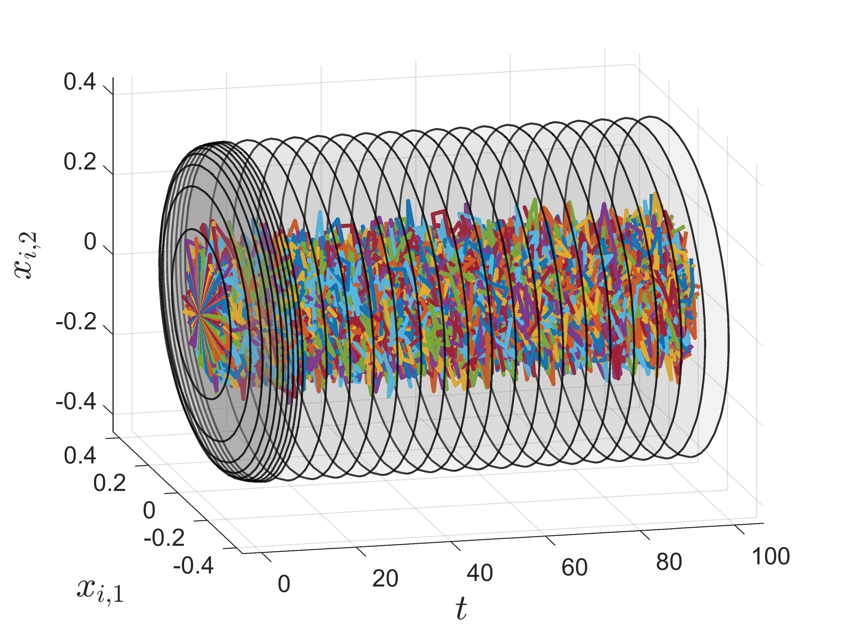
First, to transform (6) into the deterministic problem (11), we define the tighter formula $\psi$ by (9)-(10). To perform the optimizations in (10), we construct $t$-PRSs, $E_{i}(t)$, $t\in{\rm I\!N}_{[0,100]}$, for (7b) at probability levels $\theta_{i}$, $i\in{\rm I\!N}_{[1,10]}$, such that $\Pi_{i=1}^{10}\left(1-100(1-\theta_{i})\right)\geq 0.7$, and select $\theta_{i}=1-\frac{1-0.7^{\frac{1}{10}}}{100}=0.9996$ $\forall i\in{\rm I\!N}_{[1,10]}$, by homogeneity. Since $w_{i}(t)$ is zero-mean Gaussian with covariance $Q_{i}=0.05I_{2}$, $\mathscr{E}_{\theta_{i}}(\mathcal{D}(w_{i}(t))=\{w_{i}|w_{i}^{\intercal}Q_{i}^{-1}w_{i}\leq\chi_{2}^{2}(\theta_{i})\}$, where $\chi_{2}^{2}$ is the chi-squared distribution of degree $2$, is an ellipsoidal CR for $w_{i}(t)$ at probability level $\theta_{i}$. Then, we compute $E_{i}(t)$, $t\in{\rm I\!N}_{[0,100]}$, recursively by $E_{i}(t+1)=\bar{A}_{i}E_{i}(t)\oplus\mathscr{E}_{\theta_{i}}(\mathcal{D}_{w_{i}})$, with $E_{i}(0)=\{0\}$. The closed-loop matrix $\bar{A}_{i}=I_{2}+K_{i}$, where we select $K_{i}=-0.5I_{2}$, for $i\in{\rm I\!N}_{[1,10]}$. The sets $E_{i}(t)$, $t\in{\rm I\!N}_{[0,100]}$, are shown in Fig. 2. Note that, by Theorem 1, our selections of $\theta_{i}$, $i\in{\rm I\!N}_{[1,10]}$, guarantee that $\bm{E}=E(0)\times\cdots\times E(100)$, with $E(t)=E_{1}(t)\times\cdots\times E_{10}(t)$, $t\in{\rm I\!N}_{[0,100]}$, is a PRT for (8b) at probability level $\Theta=0.7$.

Refer to caption
Figure 2: Trajectories for (7b) lying in $\bm{E}_{i}=E_{i}(0)\times\cdots\times E_{i}(100)$, with probability $\Theta_{i}\geq 1-100(1-\theta_{i})=0.965$.

After we have derived $\psi$, we formulate (11) as an MILP using the YALMIP toolbox [20], in MATLAB. However, possibly due to the high dimensionality of the problem, the GUROBI solver [21] could not return a solution in a reasonable time. As a remedy, we implement the iterative optimization procedure presented in Section III-C, after decomposing $\psi$ according to (13), based on the sets $\mathcal{T}_{1}=\{(2,3),5\}$, $\mathcal{T}_{2}=\{(1,3)\}$, $\mathcal{T}_{3}=\{(1,2),4\}$, $\mathcal{T}_{4}=\{3,5\}$, $\mathcal{T}_{5}=\{1,4,6\}$, $\mathcal{T}_{6}=\{5,8,9\}$, $\mathcal{T}_{7}=\{4,8\}$, $\mathcal{T}_{8}=\{6,7,10\}$, $\mathcal{T}_{9}=\{6,10\}$, and $\mathcal{T}_{10}=\{8,9\}$. By selecting sets $\mathcal{O}_{k}$, $k>1$, as $\mathcal{O}_{1}=\{1,4,6,10\}$, $\mathcal{O}_{2}=\{3,5,7,9\}$, $\mathcal{O}_{3}=\{8,9,2,5\}$, $\mathcal{O}_{4}=\mathcal{O}_{1}$, $\mathcal{O}_{5}=\mathcal{O}_{2}$, $\mathcal{O}_{6}=\mathcal{O}_{3}$, $\mathcal{O}_{7}=\mathcal{O}_{1}$, and so on, we run Algorithm 1, which terminates after seven iterations returning a multi-agent trajectory that satisfies the global STL task $\psi$. Computational aspects of Algorithm 1 are depicted in Fig. 3 (left), while Fig. 3 (right) illustrates the evolution of the robustness function computed at the agent level during the execution of Algorithm 1. Fig. 4 displays $10^{3}$ realizations of noisy multi-agent trajectories, illustrating also the impact of constraint tightening on the workspace $\mathcal{X}$, obstacles $O_{1}$, $O_{2}$, $O_{3}$, and the regions $T_{i}$, $G_{i}$ ($i\in{\rm I\!N}_{[1,10]}$). By evaluating the robustness function of the global STL specification $\phi$ for numerous noisy realizations, we see that $\phi$ is violated in less than $30\%$ of the total realizations, verifying Theorem 2.

$10^{1}$ $10^{2}$Runtime (s)
$2$ $4$ $6$ $-15$ $-10$ $-5$00Iterations$\rho^{\hat{\psi}_{i}}$12345678910
Figure 3: (Left) Compute time distribution for computations performed on an i7-1185G7 CPU at 3.00GHz. (Right) Robustness function of local formula $\hat{\psi}_{i}$ evaluated per iteration.
Refer to caption
Figure 4: $10^{3}$ realizations of the MAS with initial conditions $x_{1}(0)=(1.5,10)$, $x_{2}(0)=(1.5,15)$, $x_{3}(0)=(11.5,10)$, $x_{4}(0)=(13.5,10)$, $x_{5}(0)=(15.5,10)$, $x_{6}(0)=(31.5,10)$, $x_{7}(0)=(33.5,10)$, $x_{8}(0)=(36.5,10)$, $x_{9}(0)=(47,10)$, $x_{10}(0)=(47,15)$, and effect of tightening in $\mathcal{X}$, $O_{1}$, $O_{2}$, $O_{3}$, and $T_{i}$, $G_{i}$, $i\in{\rm I\!N}_{[1,10]}$.

V Conclusion

We have addressed the control synthesis of stochastic multi-agent systems under STL specifications formulated as probabilistic constraints. Leveraging linearity, we extract the stochastic component from the MAS dynamics for which we construct a PRT at probability level bounded by the specification probability. We use segments of this PRT to define a tighter STL formula and convert the underlying stochastic optimal control problem into a deterministic one with a tighter domain. Our PRT-based tightening reduces conservatism compared to approaches relying on the STL specification structure. To enhance scalability, we propose a recursively feasible iterative procedure where the resulting problem is decomposed into agent-level subproblems, reducing its complexity. Although our method fits a large-scale MAS setting, the conservatism introduced by the construction of PRTs increases with the specification horizon. This will be addressed in future work by utilizing more efficient, sampling-based techniques, avoiding union-bound arguments.

References

  • [1] S. S. Farahani, R. Majumdar, V. S. Prabhu, and S. Soudjani, “Shrinking horizon model predictive control with signal temporal logic constraints under stochastic disturbances,” IEEE TAC, vol. 64, no. 8, pp. 3324–3331, 2019.
  • [2] Z. Liu, B. Wu, J. Dai, and H. Lin, “Distributed communication-aware motion planning for multi-agent systems from stl and spatel specifications,” in IEEE CDC, 2017, pp. 4452–4457.
  • [3] A. T. Buyukkocak, D. Aksaray, and Y. Yazıcıoğlu, “Planning of heterogeneous multi-agent systems under signal temporal logic specifications with integral predicates,” IEEE Rob. and Autom. Letters, vol. 6, no. 2, pp. 1375–1382, 2021.
  • [4] O. Maler and D. Nickovic, “Monitoring Temporal Properties of Continuous Signals,” in Formal Techniques, Modelling and Analysis of Timed and Fault-Tolerant Systems, Y. Lakhnech and S. Yovine, Eds.   Berlin, Heidelberg: Springer Berlin Heidelberg, 2004, pp. 152–166.
  • [5] V. Raman, M. Maasoumy, A. Donze, R. M. Murray, A. Sangiovanni-Vincentelli, and S. A. Seshia, “Model predictive control with signal temporal logic specifications,” in Proceedings of the IEEE Conf. on Decis. and Cont.   IEEE, 2014, pp. 81–87.
  • [6] A. Donzé and O. Maler, “Robust Satisfaction of Temporal Logic over Real-Valued Signals,” in 8th International Conference on Formal Modeling and Analysis of Timed Systems, FORMATS, 2010, Klosterneuburg, Austria, 2010, pp. 92–106.
  • [7] S. Safaoui, L. Lindemann, D. V. Dimarogonas, I. Shames, and T. H. Summers, “Control Design for Risk-Based Signal Temporal Logic Specifications,” IEEE L-CSS, vol. 4, no. 4, pp. 1000–1005, 2020.
  • [8] L. Lindemann, G. J. Pappas, and D. V. Dimarogonas, “Control Barrier Functions for Nonholonomic Systems under Risk Signal Temporal Logic Specifications,” in Proceedings of the IEEE Conf. on Decis. and Cont., 2020, pp. 1422–1428.
  • [9] ——, “Reactive and Risk-Aware Control for Signal Temporal Logic,” IEEE Trans. Autom. Control, vol. 67, no. 10, pp. 5262–5277, 2022.
  • [10] D. Sadigh and A. Kapoor, “Safe Control under Uncertainty with Probabilistic Signal Temporal Logic,” in Proceedings of Robotics: Science and Systems, jun 2016.
  • [11] S. Jha, V. Raman, D. Sadigh, and S. A. Seshia, “Safe Autonomy Under Perception Uncertainty Using Chance-Constrained Temporal Logic,” Journal of Automated Reasoning, vol. 60, no. 1, pp. 43–62, 2018.
  • [12] J. Li, P. Nuzzo, A. Sangiovanni-Vincentelli, Y. Xi, and D. Li, “Stochastic contracts for cyber-physical system design under probabilistic requirements,” in MEMOCODE 2017 - 15th ACM-IEEE International Conference on Formal Methods and Models for System Design, 2017, pp. 5–14.
  • [13] P. Kyriakis, J. V. Deshmukh, and P. Bogdan, “Specification mining and robust design under uncertainty: A stochastic temporal logic approach,” ACM Trans. on Emb. Comp. Syst., vol. 18, no. 5s, 2019.
  • [14] G. Scher, S. Sadraddini, R. Tedrake, and H. Kress-Gazit, “Elliptical slice sampling for probabilistic verification of stochastic systems with signal temporal logic specifications,” in Proceedings of the 25th ACM International Conference on Hybrid Systems: Computation and Control, ser. HSCC ’22.   New York, NY, USA: Association for Computing Machinery, 2022.
  • [15] G. Scher, S. Sadraddini, and H. Kress-Gazit, “Robustness-based synthesis for stochastic systems under signal temporal logic tasks,” in IEEE IROS, 2022, pp. 1269–1275.
  • [16] T. Yang, Y. Zou, S. Li, and Y. Yang, “Distributed model predictive control for probabilistic signal temporal logic specifications,” IEEE Trans. on Autom. Sc. and Eng., pp. 1–11, 2023.
  • [17] L. Hewing, A. Carron, K. P. Wabersich, and M. N. Zeilinger, “On a correspondence between probabilistic and robust invariant sets for linear systems,” in ECC, 2018, pp. 1642–1647.
  • [18] J. Orlin, “Contentment in graph theory: Covering graphs with cliques,” Indagationes Mathematicae, vol. 80, no. 5, pp. 406–424, 1977.
  • [19] E. E. Vlahakis, L. Lindemann, and D. V. Dimarogonas, “Distributed sequential receding horizon control of multi-agent systems under recurring signal temporal logic,” arXiv:2311.06890v1, 2023.
  • [20] J. Löfberg, “Yalmip : A toolbox for modeling and optimization in matlab,” in In Proceedings of the CACSD Conference, Taiwan, 2004.
  • [21] “Gurobi optimizer,” https://www.gurobi.com, 2023.