Authentic Majorana versus singlet Dirac neutrino contributions to $\mu^{-}\mu^{-}\to\ell^{-}\ell^{-}$ $(\ell=e,\tau)$ transitions

Abstract

We revisited the computation of the cross section for the $\mu^{-}\mu^{-}\to\ell^{-}\ell^{-}$ $(\ell^{-}=\tau^{-},\,e^{-})$ transitions in the presence of new heavy Majorana neutrinos. We focus on scenarios where the masses of the new states are around some few TeV, the so-called low-scale seesaw models. Our analysis is set in a simple model with only two new heavy Majorana neutrinos considering the current limits on the heavy-light mixings. Our results illustrate the difference between the genuine effects of two nondegenerate heavy Majorana states and the degenerate case where they form a Dirac singlet field.

I Introduction

The evidence of neutrino oscillation phenomena [1, 2, 3] establishes mixing in the leptonic sector that, for three lepton families, is parameterized by the ($3\times 3$) unitary PMNS matrix [4, 5], analogous to the CKM matrix in the quark sector [6, 7]. Furthermore, the neutrino oscillation phenomena demand an explanation of the origin and nature of neutrino masses. One of the simplest models to address these questions is the so-called $\nu$SM [8], which introduces singlet right-handed components for neutrino states and generates their masses after spontaneous symmetry breaking via Yukawa couplings with the Higgs field in a manner completely analogous to the rest of the fermions. However, the $\nu$SM would require tiny Yukawa couplings to account for the observed neutrino masses.

Additionally, since the neutrino right-handed fields are Standard Model (SM) singlets, they may introduce Majorana mass terms, which could define a new energy scale and suggest the possibility of an alternative mass-generation mechanism. This is the idea behind the so-called high seesaw scenarios, where the tininess of neutrino masses is owing to the tree-level exchange of very heavy fields, such as right-handed singlet fermions (type-I seesaw) [9, 10, 11, 12], scalar triplets (type-II seesaw) [13, 14, 15, 16, 17], or fermion triplets (type-III seesaw) [18].

On the other hand, another consequence of neutrino oscillation is the fact that lepton flavor is not conserved, at least in the neutrino sector. Furthermore, massive neutrinos will induce charged lepton flavor violation (cLFV) at the one-loop level, even though these processes have never been observed. This fact can be well explained in minimal massive neutrino models such as the two previously mentioned, namely, the $\nu$SM and type-I seesaw models. In the former, there is a suppression factor of $(m_{\nu}/E)^{2}$ (with $E$ as the scale of the processes) for the contribution of the light active neutrinos, while in the latter, the contributions of the new heavy sector have a suppression of the order $(E/m_{N})^{2}$ in the heavy-light mixing of the heavy states, which is equally small.

In contrast, cLFV can emerge considerably in other well-motivated extensions. Therefore, searching for cLFV processes is one of the most compelling ways to reveal new physics. Nowadays, the so-called three ’golden’ cLFV processes—$\mu\to e\gamma$, $\mu\to e\bar{e}e$, and $\mu-e$ conversion—set limits with sensitivities of the order $10^{-13}$ for the former two and $10^{-12}$ for the latter process [19, 20, 21], respectively. Nevertheless, a completely new generation of experiments would be able to considerably improve such limits. Specifically, the MEG-II, Mu3e, and PRISM (COMET) collaborations will reach sensitivities of $6\times 10^{-14}$ [22, 23] for $\mu\to e\gamma$, $10^{-16}$ [24] for $\mu\to e\bar{e}e$, and $10^{-18}$ [25] for $\mu-e$(Ti) conversion ($10^{-17}$ [26] for $\mu-e$(Al) conversion), respectively .

Additionally, the potential advent of muon colliders [48, 49, 50, 51, 52, 53, 54] opens another route for complementary searches of NP, including cLFV processes [55, 56, 57, 58, 59]. This idea includes the possibility of both muon-antimuon ($\mu^{-}\mu^{+}$) [48, 49, 50, 51, 60] and same-sign ($\mu^{-}\mu^{-}$) muon colliders [61, 62, 63, 64, 65] with a center-of-mass energy in the TeV scale. Motivated by this, in this work, we compute the cross section for the $\mu^{-}\mu^{-}\to\ell^{-}\ell^{-}$ ($\ell^{-}=\tau^{-},\,e^{-}$) transitions in scenarios that introduce new heavy neutrino states. Our attention is focused on models with massive Majorana neutrinos around the TeV scale. Furthermore, our results address some comments on previous computations for the $e^{-}e^{-}\to\mu^{-}\mu^{-}$ [66] and $\mu^{-}\mu^{-}\to\ell^{-}\ell^{-}$ ($\ell^{-}=\tau^{-},\,e^{-}$) channels [67]. In those previous works, only the contributions of one-loop box diagrams with explicit lepton number-violating (LNV) vertices are included. However, we highlight that an accurate estimation requires another set of diagrams, omitted in Refs. [66, 67] .

The manuscript is structured as follows: Section II introduces a simple model that captures all the relevant effects of new heavy neutrinos to cLFV transitions. This minimal scenario will allow us to estimate the genuine effects of two nondegenerate Majorana states and compare it with the degenerate case, where they define a Dirac singlet field. After that, section III is devoted to the meaningful aspect of our computation introducing the $\mu^{-}\mu^{-}\to\ell^{-}\ell^{-}$ ($\ell=e,\,\tau$) one-loop amplitudes in massive neutrino models (some important details and identities used in our computation are left to the appendix). Then section IV estimates the total cross-section for these processes based on both the current limits of the heavy-light mixings and a perturbative condition. Finally, the conclusions and a summary of our results are presented in section V.

II The model

We work in a simplified model previously presented in Refs. [68, 69]. Here, the neutrino sector is composed of five self-conjugate states whose left-handed components $\chi_{Li}$ include the three active neutrinos ($i=1,2,3$) plus two sterile spinors $\chi_{\{4,5\}}$ of opposite lepton number. The Lagrangian defining the neutrino masses is assumed to have the form:

$$-\mathcal{L}\supset\,\sum_{i}^{3}Y_{i}\Phi^{\dagger}L_{i}\overline{\chi_{5}^{c}}+M\,\overline{\chi_{5}^{c}}\chi_{4}+\frac{1}{2}\mu\,\overline{\chi}_{5}\chi_{5}^{c}+\textrm{h.c.}\,,$$ (II.1)

where $\Phi$ and $L_{i}$ are the Higgs and lepton SM doublets, respectively; whereas $Y_{i}$ corresponds to Yukawa couplings. After the spontaneous electroweak symmetry breaking, the neutrino mass matrix is written as:

$$\mathcal{M^{\nu}}=\left(\begin{tabular}[]{ccccc}$0$&$0$&$0$&$0$&$m_{1}$\\ $0$&$0$&$0$&$0$&$m_{2}$\\ $0$&$0$&$0$&$0$&$m_{3}$\\ $0$&$0$&$0$&$0$&$M$\\ $m_{1}$&$m_{2}$&$m_{3}$&$M$&$\mu$\\ \end{tabular}\right),$$ (II.7)

with the masses $m_{i}\equiv Y_{i}v/\sqrt{2}$ for ($i=1,2,3$), and $v\approx 256\,$GeV the vacuum expectation value (VEV) of the Higgs field. The diagonalization of Eq. (II.7) leads to three massless neutrinos $\nu_{i}$ and two heavy neutrino states with masses

$$m_{\{N_{1},N_{2}\}} =\frac{1}{2}\left(\sqrt{4(m^{2}+M^{2})+\mu^{2}}\pm\mu\right)\,,$$ (II.8)

with the definition $m^{2}\equiv m_{1}^{2}+m_{2}^{2}+m_{3}^{2}$.

On the other hand, the weak charged lepton currents necessary for computing the cLFV processes are described by [68, 69] (arising, at one-loop level, through the mixing of the leptonic sector)

$$\mathcal{L}_{W^{\pm}}=-\frac{g}{\sqrt{2}}W_{\mu}^{-}\sum_{i=1}^{3}\sum_{j=1}^{5}B_{ij}\,\bar{\ell}_{i}\gamma_{\mu}P_{L}\chi_{j}+\textrm{h.c.}\,.$$ (II.9)

Working in the Feynman-’t Hooft gauge would also require considering the interaction of the unphysical charged Goldstone bosons with a pair of leptons, those vertices are described by [68, 69]

$$\mathcal{L}_{G^{\pm}}=-\frac{g}{\sqrt{2}}G^{-}\sum_{i=1}^{3}\sum_{j=1}^{5}B_{ij}\,\bar{\ell}_{i}\left(\frac{m_{\ell_{i}}}{M_{W}}P_{L}-\frac{m_{X_{j}}}{M_{W}}P_{R}\right)\chi_{j}+\textrm{h.c.}\,.$$ (II.10)

In the above expressions, $B_{ij}$ is a rectangular $3\times 5$ matrix defining the mixing in the leptonic sector. The elements involving the heavy new states $N_{1,2}$ are crucial in the description of both lepton number violating (LNV) and cLFV effects, they can be written as:

$$B_{kN_{1}}=-i\frac{r^{1/4}}{\sqrt{1+r^{1/2}}}s_{\nu_{k}},\quad B_{kN_{2}}=\frac{1}{\sqrt{1+r^{1/2}}}s_{\nu_{k}},$$ (II.11)

with the definition $r\equiv m_{N_{2}}^{2}/m_{N_{1}}^{2}$, and $s_{\nu_{k}}$ ($k=e,\,\mu,\,\tau$) define the angles of the heavy states with the three flavors, they are expressed as follows

$$s_{\nu_{k}}^{2}=\frac{m_{k}}{\sqrt{m_{N_{1}}m_{N_{2}}}}.$$ (II.12)

Something appealing about this scenario is that all the phenomenology of the leptonic mixing is described in terms of only five independent parameters, namely; a heavy mass $m_{N_{1}}$, the ratio $r$ and the three heavy-light mixings $s_{\nu_{k}}$.

It is important to mention that this is a simplified model unable to explain the masses and mixings of the light active neutrinos, however, it suffices to describe the main motivation of this work, namely, the study of cLFV effects in the presence of new heavy neutrino states with masses around $\mathcal{O}$(TeV). As already mentioned, this parametrization allows us to describe the effects of two heavy Majorana states and compare their contribution with the case of two degenerate neutrino states defining a singlet Dirac field $(r=1)$. We address this point in detail in section IV providing an estimation of the maximal total cross-section (consistent with the current limits on the heavy-light mixings) for both cases.

III Computation

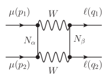
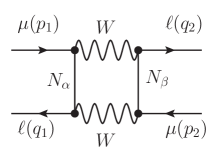
(a)	(b)

Figure 1: Feynman diagrams for the $\mu^{-}(p_{1})\mu^{-}(p_{2})\to\ell^{-}(q_{1})\ell^{-}(q_{2})$ $(\ell=e,\,\tau)$ transitions in the presence of heavy Majorana neutrinos. Working in the Feynman-’t Hooft gauge must include the four possible diagrams for the (a) and (b) contributions involving the $W$’s gauge bosons and the scalar-charged Goldstone vertices, see Appendix A.

In the presence of heavy Majorana neutrino states, Fig. 1 shows the two kinds of one-loop box diagrams contributing to the processes $\mu^{-}(p_{1})\mu^{-}(p_{2})\to\ell^{-}(q_{1})\ell^{-}(q_{2})$ ($\ell=e,\,\tau$). We will refer to diagrams (a) as those diagrams introducing explicit LNV vertices. However, for Majorana states, a complete computation must involve also the contribution of diagrams (b) . Therefore, in contrast with previous works [66, 67] that include only diagram (a) contributions, we incorporate the (b) contributions remarking their importance for an accurate estimation of the $\mu^{-}\mu^{-}\to\ell^{-}\ell^{-}$ ($\ell=e,\,\tau$) cross section. We work in the approximation where the masses of the external charged leptons are neglected . After some algebraic steps and the use of some Fierz identities (see Appendix A for further details), we have verified that the total amplitude $\mathcal{M}=\mathcal{M}_{(a)}+\mathcal{M}_{(b)}$ can be expressed in a very simple form as follows

$$\mathcal{M}=\frac{\alpha_{W}}{16\pi}\frac{e^{2}}{s_{W}^{2}}F(s,t)\,\Gamma_{L}\odot\Gamma^{R},$$ (III.1)

where $e$ is the electric charge, $\alpha_{W}\equiv\alpha/s_{W}^{2}$ with $\alpha$ the fine structure constant, and $s_{W}^{2}\equiv\sin^{2}\theta_{W}$ the Weinberg angle. We also have introduced the notation

$$\Gamma_{L}\odot\Gamma^{R}\equiv[\bar{v}(p_{1})P_{L}u(p_{2})][\bar{u}(q_{1})P_{R}v(q_{2})],$$ (III.2)

denoting a bi-spinor product, where $P_{L,R}=(1\mp\gamma_{5})/2$ stand for the chirality projectors. The $F(s,t)$ function, in Eq. (III.1) is given as follows

$$F(s,t) =\sum_{\alpha,\beta=1}^{5}\bigg{[}(B_{\mu\alpha}^{*}B_{\ell\beta})^{2}\,(\mathcal{A}+\mathcal{A}^{\prime})-2B_{\ell\alpha}B_{\mu\alpha}^{*}B_{\ell\beta}B_{\mu\beta}^{*}\,\left(\mathcal{B}+\mathcal{B}^{\prime}\right)\bigg{]},$$ (III.3)

where the factors $\mathcal{A}$, $\mathcal{A}^{\prime}$, $\mathcal{B}$, and $\mathcal{B}^{\prime}$ encode all the relevant one-loop tensor integrals given in terms of the Passiarino-Veltman functions (see Appendix B), they depend on two invariants, namely, $s=(p_{1}+p_{2})^{2}$ and $t=(p_{1}-q_{2})^{2}$; and the masses of the internal particles involved in the loop computation.

Taking the square of the amplitude in Eq. (III.1), it is straightforward to verify that the differential cross-section for the $\mu^{-}(p_{1})\mu^{-}(p_{2})\to\ell^{-}(q_{1})\ell^{-}(q_{2})$ $(\ell=e,\,\tau)$ transitions can be written as follows

$$\frac{d\sigma}{dt}=\frac{1}{2}\,\frac{1}{64\pi}\left(\frac{\alpha_{W}}{16\pi}\frac{e^{2}}{s_{W}^{2}}\right)^{2}\,|F(s,t)|^{2}\,,$$ (III.4)

where the $1/2$ factor comes from the statistical property of having two indistinguishable particles in the final state and the invariant $t$ is evaluated in the range:

$$t_{max(min)}=m_{\mu}^{2}+m_{\ell}^{2}-\frac{s}{2}\pm\frac{\lambda^{1/2}(s,m_{\mu}^{2},m_{\mu}^{2})\lambda^{1/2}(s,m_{\ell}^{2},m_{\ell}^{2})}{2s}\,,$$ (III.5)

with $\lambda(x,y,z)=x^{2}+y^{2}+z^{2}-2(xy+xz+yz)$ the so-called Källen function .

IV Numerical Evaluation

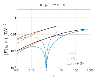
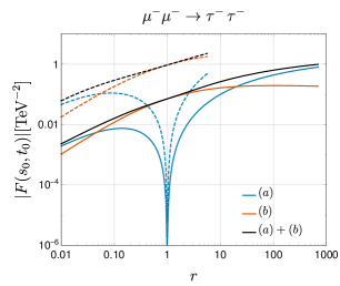
(a)	(b)

Figure 2: $F(s,t)$ factor in terms of the mass splitting $r\equiv m_{N_{2}}^{2}/m_{N_{1}}^{2}$ of the two new heavy states. The heavy-light mixings are fixed by their maximum values according to expression (IV.1), and we also have considered that $(\sqrt{s_{0}},\sqrt{|t_{0}|})=(6,0.1)$ TeV. The left (right) side of the figure illustrates the $\mu^{-}\mu^{-}\to e^{-}e^{-}$ $(\tau^{-}\tau^{-})$ channel, where the behavior of the (a) and (b) contributions are represented by the cyan and orange lines, respectively; whereas the black line stands for the total contribution. The solid (dashed) line depicts a fixed value for $m_{N_{1}}=6$ ($20$) TeV.

We now present an estimation for the $\mu^{-}\mu^{-}\to\ell^{-}\ell^{-}$ ($\ell=e,\,\tau$) cross-section in the presence of heavy Majorana neutrinos. We have considered the current experimental upper limits presented in Ref. [71] for the values of the heavy-light mixings

$$s_{\nu_{e}}<4.3\times 10^{-3},\quad s_{\nu_{\mu}}<1.61\times 10^{-2},\quad s_{\nu_{\tau}}<2.1\times 10^{-2}.$$ (IV.1)

Furthermore, we considered a perturbative limit assuming that the Yukawa couplings must satisfy the condition $|Y_{i}|^{2}<4\pi$. In our framework, this translates into the relation

$$r_{max}=\left(\frac{v\,\sqrt{2\pi}}{m_{N_{1}}\,\rm{max}\{s_{\nu_{i}}\}}\right)^{4}.$$ (IV.2)

Then considering Eqs. (IV.1) and (IV.2) we plot in Fig. 2 the relevant $F(s,t)$ factor in terms of the mass splitting $r$ of the two new heavy states. Here, we used the maximum values from Eq. (IV.1) for the heavy-light mixings, along with a fixed point in the integration phase space set at $(\sqrt{s_{0}},\sqrt{|t_{0}|})=(6,0.1)$ TeV. In Fig. 2(a), the left (right) side illustrates the $\mu^{-}\mu^{-}\to e^{-}e^{-}$ $(\tau^{-}\tau^{-})$ channel, where the contributions of (a) and (b) are depicted by cyan and orange colors, respectively. Meanwhile, the black lines denote the total contribution, with solid (dashed) lines indicating the value for $m_{N_{1}}=6$ ($20$) TeV. Some noteworthy observations from this figure are as follows:

It turns out clear that in the limit when $r\to 1$, the (a) contributions tend to zero, as expected, since in such a case the two new heavy states are degenerate forming a Dirac singlet field and recovering lepton number as a symmetry of our model. In such a case, the cross-section for the $\mu^{-}\mu^{-}\to\ell^{-}\ell^{-}$ ($\ell=e,\,\tau$) transitions would be determined exclusively by the diagrams (b). This is a different result to previous estimations in [66, 67] where the contributions (b) were omitted. Note that for $m_{N_{1}}=6$ TeV and $r$ in the range $(0.1,10)$, the contributions (a) consistently remain below those from diagrams (b), and only for values of $r\gtrsim 11$ the contributions (a) become dominant. Moreover, if we consider both the maximum values in (IV.1) for the heavy-light mixings and $m_{N_{1}}=20$ TeV, then the upper limit of $r$ consistent with Eq. (IV.2) would be $r_{max}=4.64$ (this is depicted in Fig. 2 where the dashed lines end).

Additionally, Fig. 2(b) illustrates a suppression of approximately two orders of magnitude for $\mu^{-}\mu^{-}\to e^{-}e^{-}$ in comparison with the $\mu^{-}\mu^{-}\to\tau^{-}\tau^{-}$. This difference arises from the more restrictive experimental limits of the heavy-light mixings in Eq. (IV.1) involving electrons. Therefore, we will concentrate on the $\mu^{-}\mu^{-}\to\tau^{-}\tau^{-}$ channel.

In Figure 3(a) we integrate Eq. (III.4) over the $t$ invariant to plot the total cross-section as a function of the invariant mass $\sqrt{s}$. Here, we have considered the mass of the heavy neutrino to be $m_{N_{1}}=20$ TeV and $r_{\text{max}}=4.64$ consistent with Eq. (IV.2). We observe from this that taking an energy of collision around $\sqrt{s}\approx 6$ TeV, the maximal cross-section for the $\mu^{-}\mu^{-}\to\tau^{-}\tau^{-}$ channel would be of the order $\mathcal{O}(10^{-2})$ fb. Thus, if we consider the expected sensitivity reported in reference [63] for an expected total integrated luminosity (at $\sqrt{s}=6$ TeV) of around 12 fb^-1 year^-1, we would have approximately one $\mu^{-}\mu^{-}\to\tau^{-}\tau^{-}$ event for every nine years of collisions. Nevertheless, following a more optimistic scenario, as presented in Ref. [64], where the authors study similar transitions in the type-II seesaw model. If we consider an integrated luminosity of $10$ ab^-1 with the center of mass energy $\sqrt{s}=10$ TeV, we estimated around $300$ events for the $\mu^{-}\mu^{-}\to\tau^{-}\tau^{-}$ channel in low scale seesaw models with masses of the new neutrinos around some TeV, as presented in Fig. 3(a).

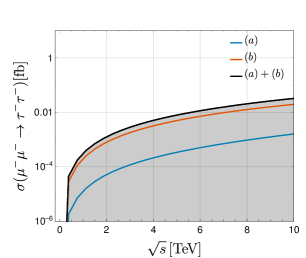
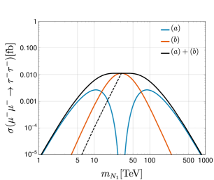
(a)	(b)

Figure 3: Left (Right): Cross-section of the $\mu^{-}\mu^{-}\to\tau^{-}\tau^{-}$ transition as a function of $\sqrt{s}$ ($m_{N_{1}}$). The contributions of diagrams (a) and (b) are represented by the cyan and orange lines, respectively. The black lines stand for the total contribution. In the left plot, we have considered $m_{N_{1}}=20$ TeV and $r_{\text{max}}=4.64$ consistent with Eq. (IV.2). The shadow area here represent the cross-section considering the heavy-light mixings below the current limits in expression (IV.1) and $r<r_{\textrm{max}}$.

It is also important to stress that from a phenomenological point of view, these processes would be crucial to compare the genuine effects of heavy Majorana states with the contributions of new heavy Dirac singlets. In this regard, Fig. 3(b) depicts the behavior of the cross-section as a function of the heavy neutrino mass $m_{N_{1}}$ considering a transferred energy of $\sqrt{s}=6$ TeV, and $r=r_{max}$ (solid black lines) . The cyan and orange lines stand for the contributions of diagrams (a) and (b), respectively. Note that since the black line consistently lies above both the orange and cyan lines, the contributions of diagrams (a) and (b) in Figure 1 interfere constructively.

From Figure 3(b), we can also see that for $m_{N_{1}}<13$ TeV and $m_{N_{1}}>65$ TeV, the dominant contribution arises from diagrams (a), which introduce explicit lepton number violation (LNV) vertices. Conversely, for $m_{N_{1}}$ within the interval $(13,65)$ TeV, diagrams (b) become dominant, reaching a maximum of around $10^{-2}$ fb for $m_{N_{1}}\approx(20-50)$ TeV. Note that the cyan line tends towards zero as $m_{N_{1}}$ approaches 32 TeV because this corresponds to the scenario where $r_{\text{max}}=1$ and diagram (a) vanishes, as discussed previously. Finally, for comparative purposes, we include the Dirac singlet scenario ($r=1$), indicated by the black dashed line. In this case, $m_{N_{1}}<31$ TeV since beyond this range, $r=1$ contradicts eq.(IV.2). An important point to highlight here is that even in the absence of lepton number violation (LNV) in the theory, we still obtain non-zero values of the cross-section, reaching up to the limit of $\sigma\approx 10^{-2}$ fb.

V Conclusions

Some experimental collaborations expect to substantially improve the current limits on an extensive list of cLFV processes, including leptonic, hadron, and heavy boson decays [22, 23, 24, 25, 26]. These searches will either provide thrilling indications of new physics or impose even more stringent limits on extensions to the Standard Model.

In this work, motivated by the potential of future muon colliders, we investigate the $\mu^{-}\mu^{-}\to\ell^{-}\ell^{-}$ $(\ell=\tau,\,e)$ processes as part of complementary cLFV searches. We calculate the complete cross-section for these processes within scenarios featuring new heavy Majorana states. Our analysis is based on a setup involving only two new heavy Majorana neutrinos, while taking into account the current constraints on their mixings with the light sector.

Our results shows that the observation of the $\mu^{-}\mu^{-}\to\tau^{-}\tau^{-}$ cLFV transition due to the presence of new heavy Majorana neutrinos (with masses around $m_{N_{1}}\approx 20$ TeV) in low scale seesaw models could be possible in a future same-sign muon collider only in the case of an energy of collision $\sqrt{s}\gtrsim 10$ TeV and an integrated luminosity of order $\mathcal{O}(\rm{ab}^{-1})$. We also underscore the importance of considering both (a) and (b) contributions to estimate the $\mu^{-}\mu^{-}\to\ell^{-}\ell^{-}$ cross-section accurately. Whether the dominant contribution arises from diagrams (a) with explicit LNV or not depends on the specific values of the $(m_{N_{2}},m_{N_{1}})$ masses of the new Majorana neutrinos. This distinction is crucial in distinguishing between the scenario with two nondegenerate heavy Majorana states and the degenerate case where they form a Dirac singlet field.

Appendix A Amplitudes

Before presenting the amplitudes of diagrams in Fig 1, let us introduce the following notation to avoid cumbersome expressions:

$$\Gamma_{X}^{\{1,\mu,\mu\nu\}}\odot\Gamma^{Y}_{\{1,\alpha,\alpha\beta\}} \equiv\left[\bar{v}(p_{1})\{1,\gamma^{\mu},\sigma^{\mu\nu}\}P_{X}u(p_{2})\right]\,\left[\bar{u}(q_{1})\{1,\gamma_{\alpha},\sigma_{\alpha\beta}\}P_{Y}v(q_{2})\right],$$ (A.1)

$$\Gamma_{X}^{\{1,\mu,\mu\nu\}}\otimes\Gamma^{Y}_{\{1,\alpha,\alpha\beta\}} \equiv\left[\bar{u}(q_{1})\{1,\gamma^{\mu},\sigma^{\mu\nu}\}P_{X}u(p_{1})\right]\,\left[\bar{u}(q_{2})\{1,\gamma_{\alpha},\sigma_{\alpha\beta}\}P_{Y}u(p_{2})\right],$$ (A.2)

where $P_{X}$ and $P_{Y}$ represent either the left or right projection operator.

A.1 Diagrams with explicit LNV vertices

The amplitudes for diagrams (a), namely, those with explicit LNV vertices can be expressed in a general form as follows

$$\mathcal{M}_{LNV}^{a_{1}a_{2}} =\frac{\alpha_{W}}{16\pi}\frac{e^{2}}{s_{W}^{2}}\sum_{\alpha,\beta}^{5}(B_{\mu\alpha}^{*}B_{\ell\beta})^{2}\,M^{a_{1}a_{2}}_{LNV},$$ (A.3)

where the superscript $a_{1}$ $(a_{2})$ denotes the contribution of the particle ($W$ gauge boson or $\phi$ Goldstone boson) in the up (down) vertices of diagrams 1(a). We have found that

$$M_{LNV}^{WW} =A_{1}\,\Gamma_{L}\odot\Gamma^{R},$$ (A.4)

$$M_{LNV}^{\phi W+W\phi} =A_{2}\,\Gamma_{L}\odot\Gamma^{R}+\Gamma_{L}^{\mu\alpha}\odot\Gamma^{R}_{\mu\beta}\left(B_{1}\,q_{2_{\alpha}}p_{1}^{\beta}+B_{2}\,q_{2_{\alpha}}p_{2}^{\beta}\right)$$

$$+\Gamma_{L}^{\mu\nu}\odot\Gamma^{R}\left(C_{1}\,p_{1_{\mu}}q_{2_{\nu}}+C_{2}\,p_{2_{\mu}}q_{2_{\nu}}\right)+C_{3}\,\Gamma_{L}\odot\Gamma^{R}_{\mu\nu}\,p_{1}^{\mu}p_{2}^{\nu},$$ (A.5)

$$M_{LNV}^{\phi\phi} =A_{3}\,\Gamma_{L}\odot\Gamma^{R}.$$ (A.6)

In the approximation limit where the masses of the external particles are identically zero, after some Dirac algebraic steps, Eq. (A.5) is simplified by using the following identities:

$$\Gamma_{L}^{\mu\alpha}\odot\Gamma^{R}_{\mu\beta}\,q_{2_{\alpha}}p_{(1,2)}^{\beta} =\pm q_{2}\cdot p_{(1,2)}\,\Gamma_{L}\odot\Gamma^{R},$$ (A.7)

$$\Gamma_{L}^{\mu\nu}\odot\Gamma^{R}\,p_{(1,2)_{\mu}}q_{2_{\nu}} =\mp i\,(p_{(1,2)}\cdot q_{2})\,\Gamma_{L}\odot\Gamma^{R},$$ (A.8)

$$\Gamma_{L}\odot\Gamma_{\mu\nu}^{R}\,p_{1}^{\mu}\,p_{2}^{\nu} =-i(q_{1}-q_{2})\cdot p_{2}\,\Gamma_{L}\odot\Gamma^{R}.$$ (A.9)

Therefore, the sum of expressions (A.4), (A.5), and (A.6) is given by the simply expression

$$M_{LNV} =M_{LNV}^{WW}+M_{LNV}^{\phi W+W\phi}+M_{LNV}^{\phi\phi},$$

$$=\mathcal{A}\,\Gamma_{L}\odot\Gamma^{R}\,,$$ (A.10)

where $\mathcal{A}=\left(A_{1}+A_{2T}+A_{3}\right)$, and we also have defined

$$A_{2T} \equiv A_{2}+(q_{2}\cdot p_{1})\left(B_{1}-iC_{1}\right)+(q_{2}\cdot p_{2})\left(iC_{2}-B_{2}\right)-i(q_{1}-q_{2})\cdot p_{2}\,C_{3}.$$ (A.11)

Similarly, the sum of the diagrams exchanging the final leptons ($\ell(q_{1})\leftrightarrow\ell(q_{2}))$ in Fig. (1) is identified straightforwardly from Eq. (A.10) by the replacement $M_{LNV}\rightarrow M_{LNV}^{\prime}$, with

$$M_{LNV}^{\prime} =(-1)\mathcal{A}^{\prime}\,\Gamma_{L}\odot\Gamma^{\prime\,R}\,,$$

$$=(A_{1}^{\prime}+A_{2T}^{\prime}+A_{3}^{\prime})\Gamma_{L}\odot\Gamma^{R},$$ (A.12)

where $A^{\prime}_{i}\equiv A_{i}\,(q_{1}\leftrightarrow q_{2})$. The minus sign comes after considering the Feynman rules of Majorana fermions shown in Ref. [70]. Therefore, all the contributions of diagrams (a) is given by

$$\mathcal{M}_{(a)}=\frac{\alpha_{W}}{16\pi}\frac{e^{2}}{s_{W}^{2}}\sum_{\alpha,\beta}^{5}(B_{\mu\alpha}^{*}B_{\ell\beta})^{2}(\mathcal{A}+\mathcal{A^{\prime}})\,\Gamma_{L}\odot\Gamma^{R},$$ (A.13)

A.2 Diagram (b) contributions

The amplitudes of diagrams (b) can be written in the generic form

$$\mathcal{M}_{LNC}^{b_{1}b_{2}} =\frac{\alpha_{W}}{16\pi}\frac{e^{2}}{s_{W}^{2}}\sum_{\alpha,\beta}B_{\ell\alpha}B_{\mu\alpha}^{*}B_{\ell\beta}B_{\mu\beta}^{*}\,M^{b_{1}b_{2}}_{LNC},$$ (A.14)

with

$$M_{LNC}^{WW} =\alpha_{1}\,\Gamma^{\mu}_{L}\otimes\Gamma_{\mu}^{L}+\beta_{1}\,\Gamma^{\mu}_{L}\otimes\Gamma_{\nu}^{L}q_{2\mu}\,q_{1}^{\nu},$$ (A.15)

$$M_{LNC}^{\phi W+W\phi} =\alpha_{2}\,\Gamma^{\mu}_{L}\otimes\Gamma_{\mu}^{L},$$ (A.16)

$$M_{LNC}^{\phi\phi} =\alpha_{3}\,\Gamma^{\mu}_{L}\otimes\Gamma_{\mu}^{L}+\left(\beta_{2}\,p_{2\mu}q_{1}^{\nu}+\beta_{3}\,q_{2\mu}\,q_{1}^{\nu}\right)\,\Gamma^{\mu}_{L}\otimes\Gamma_{\nu}^{L}.$$ (A.17)

Considering the approximation where the masses of the external particles are zero, the sum of the above expressions is given by

$$M_{LNC} =M_{LNC}^{WW}+M_{LNC}^{\phi W+W\phi}+M_{LNC}^{\phi\phi},$$

$$=\mathcal{B}\,\Gamma_{L}^{\mu}\otimes\Gamma^{L}_{\mu},$$ (A.18)

where, in the above expression, we have used the identity

$$\Gamma_{L}^{\mu}\otimes\Gamma^{L}_{\nu}\,q_{2\mu}q_{1}^{\nu}=\Gamma_{L}^{\mu}\otimes\Gamma^{L}_{\nu}\,p_{2\mu}q_{1}^{\nu}=(p_{2}\cdot q_{1})\Gamma_{L}^{\mu}\otimes\Gamma^{L}_{\mu}\,$$ (A.19)

and we have defined $\mathcal{B}\equiv\alpha_{1T}+\alpha_{2}+\alpha_{3T}$, where

$$\alpha_{1T} =\alpha_{1}+(p_{2}\cdot q_{1})\beta_{1}$$ (A.20)

$$\alpha_{3T} =\alpha_{3}+(p_{2}\cdot q_{1})(\beta_{2}+\beta_{3}).$$ (A.21)

Similar to the (a) contributions, the inclusion of the diagrams with the final charged leptons exchanged is added to the amplitude after the change $q_{1}\leftrightarrow q_{2}$ in the above expressions, which takes to

$$\mathcal{M}_{(b)}=\frac{\alpha_{W}}{16\pi}\frac{e^{2}}{s_{W}^{2}}\sum_{\alpha,\beta}^{5}B_{\ell\alpha}B_{\mu\alpha}^{*}B_{\ell\beta}B_{\mu\beta}^{*}(\mathcal{B}+\mathcal{B}^{\prime})\,\Gamma_{L}^{\mu}\otimes\Gamma^{L}_{\mu}.$$ (A.22)

The sum of Eqs. (A.13) and (A.22) can be done immediately by considering the Fierz identity

$$\Gamma^{\mu}_{L}\otimes\Gamma_{\mu}^{L}=-2\Gamma_{L}\odot\Gamma^{R}.$$ (A.23)

Thus, the total contribution $\mathcal{M}=\mathcal{M}_{(a)}+\mathcal{M}_{(b)}$ is given by Eq. (III.1) .

Appendix B Loop functions

All the relevant factors coming from the loop integration presented in the previous appendix are given in terms of Passarino-Veltman (PaVe) functions. We have used the software Package X [72] for our computaion and we have found the following expression

$$A_{1} =4m_{N_{\alpha}}m_{N_{\beta}}\overline{D}_{0},$$ (B.1)

$$A_{2T} =-2\frac{m_{N_{\alpha}}m_{N_{\beta}}}{m_{W}^{2}}\bigg{[}4\overline{D}_{00}-t\left(\overline{D}_{0}+\overline{D}_{1}+2\overline{D}_{2}+\overline{D}_{3}\right.\left.+2(\overline{D}_{12}+\overline{D}_{13}+\overline{D}_{22}+\overline{D}_{23})\right)\bigg{]},$$

$$A_{3} =\frac{m_{N_{\alpha}}^{3}m_{N_{\beta}}^{3}}{m_{W}^{4}}\overline{D}_{0}.$$ (B.2)

Note that these are the same expressions obtained in Ref.[66], except for a minus sign in the eq.(B). We have introduced the following notation to express the argument of the Passarino-Veltman functions involved in the contributions of diagrams (a)

$$\overline{D}_{i}\equiv D_{i}(0,0,0,0;s,t;m_{W},m_{N_{\alpha}},m_{W},m_{N_{\beta}}).$$ (B.3)

Regarding the diagrams (b) contributions we have found the relevant expressions

$$\alpha_{1T} =4D_{00}-2t(D_{0}+D_{1}+D_{3}+D_{13})\,,$$ (B.4)

$$\alpha_{2} =-2\frac{m_{N_{\alpha}}^{2}m_{N_{\beta}}^{2}}{m_{W}^{2}}D_{0}\,$$ (B.5)

$$\alpha_{3T} =\frac{m_{N\alpha}^{2}m_{N\beta}^{2}}{2m_{W}^{2}}(2D_{00}-D_{13}),$$ (B.6)

where, this time, the arguments of the Passarino-Veltman function are given by

$$D_{i}\equiv D_{i}(0,0,0,0;u,t;m_{N_{\alpha}},m_{W},m_{N_{\beta}}).$$ (B.7)

Defining the invariant $u\equiv(p_{1}-q_{1})^{2}=(p_{2}-q_{2})^{2}$ and taking $\mathcal{A}^{\prime}$ ( $\mathcal{B}^{\prime}$) factor related with $\mathcal{A}(\mathcal{B})$ by the change $t\leftrightarrow u$ in the corresponding PaVe functions.

Appendix C Expressions in terms of the massive states

Using the neutrino’s mass framework introduced in section II, we can rearrange the sum over all the mass eigenstates shown in eq.(III.3) in terms only of the heavy states as follows

$$\sum_{\alpha,\beta=1}^{5}B_{\ell\alpha}B_{\mu\alpha}^{*}B_{\ell\beta}B_{\mu\beta}^{*}d(m_{\alpha},m_{\beta})\equiv \sum_{\alpha,\beta=4}^{5}B_{\ell\alpha}B_{\mu\alpha}^{*}B_{\ell\beta}B_{\mu\beta}^{*}\left(d(m_{\alpha},m_{\beta})-d(0,m_{\beta})\right.$$

$$\left.-d(m_{\alpha},0)+d(0,0)\right)\,,$$

where $d(m_{\alpha},m_{\beta})$ an arbitrary function that depends on the neutrino masses. It is important to remark that this simplification is valid only for this specific model where the light neutrinos have masses identically zero.

References

- [1] Y. Fukuda et al. Evidence for oscillation of atmospheric neutrinos. Phys. Rev. Lett., 81:1562–1567, 1998.
- [2] Q. R. Ahmad et al. Measurement of the rate of interactions produced by 8B solar neutrinos at the Sudbury Neutrino Observatory. Phys. Rev. Lett., 87:071301, 2001.
- [3] Q. R. Ahmad et al. Direct evidence for neutrino flavor transformation from neutral current interactions in the Sudbury Neutrino Observatory. Phys. Rev. Lett., 89:011301, 2002.
- [4] B. Pontecorvo. Inverse beta processes and nonconservation of lepton charge. Zh. Eksp. Teor. Fiz., 34:247, 1957.
- [5] Ziro Maki, Masami Nakagawa, and Shoichi Sakata. Remarks on the unified model of elementary particles. Prog. Theor. Phys., 28:870–880, 1962.
- [6] Nicola Cabibbo. Unitary Symmetry and Leptonic Decays. Phys. Rev. Lett., 10:531–533, 1963.
- [7] Makoto Kobayashi and Toshihide Maskawa. CP Violation in the Renormalizable Theory of Weak Interaction. Prog. Theor. Phys., 49:652–657, 1973.
- [8] R. N. Mohapatra and P. B. Pal. Massive neutrinos in physics and astrophysics. Second edition, volume 60. 1998.
- [9] Peter Minkowski. at a Rate of One Out of Muon Decays? Phys. Lett. B, 67:421–428, 1977.
- [10] Tsutomu Yanagida. Horizontal gauge symmetry and masses of neutrinos. Conf. Proc. C, 7902131:95–99, 1979.
- [11] Murray Gell-Mann, Pierre Ramond, and Richard Slansky. Complex Spinors and Unified Theories. Conf. Proc. C, 790927:315–321, 1979.
- [12] Rabindra N. Mohapatra and Goran Senjanovic. Neutrino Mass and Spontaneous Parity Nonconservation. Phys. Rev. Lett., 44:912, 1980.
- [13] M. Magg and C. Wetterich. Neutrino Mass Problem and Gauge Hierarchy. Phys. Lett. B, 94:61–64, 1980.
- [14] J. Schechter and J. W. F. Valle. Neutrino Masses in SU(2) x U(1) Theories. Phys. Rev. D, 22:2227, 1980.
- [15] T. P. Cheng and Ling-Fong Li. Neutrino Masses, Mixings and Oscillations in SU(2) x U(1) Models of Electroweak Interactions. Phys. Rev. D, 22:2860, 1980.
- [16] George Lazarides, Q. Shafi, and C. Wetterich. Proton Lifetime and Fermion Masses in an SO(10) Model. Nucl. Phys. B, 181:287–300, 1981.
- [17] Rabindra N. Mohapatra and Goran Senjanovic. Neutrino Masses and Mixings in Gauge Models with Spontaneous Parity Violation. Phys. Rev. D, 23:165, 1981.
- [18] Robert Foot, H. Lew, X. G. He, and Girish C. Joshi. Seesaw Neutrino Masses Induced by a Triplet of Leptons. Z. Phys. C, 44:441, 1989.
- [19] J. Adam et al. New constraint on the existence of the decay. Phys. Rev. Lett., 110:201801, 2013.
- [20] U. Bellgardt et al. Search for the Decay . Nucl. Phys. B, 299:1–6, 1988.
- [21] Wilhelm H. Bertl et al. A Search for muon to electron conversion in muonic gold. Eur. Phys. J. C, 47:337–346, 2006.
- [22] A. M. Baldini et al. The design of the MEG II experiment. Eur. Phys. J. C, 78(5):380, 2018.
- [23] G. Cavoto, A. Papa, F. Renga, E. Ripiccini, and C. Voena. The quest for and its experimental limiting factors at future high intensity muon beams. The European Physical Journal C, 78(1):37, 2018.
- [24] A. Blondel et al. Research Proposal for an Experiment to Search for the Decay . 1 2013.
- [25] A. Alekou et al. Accelerator system for the PRISM based muon to electron conversion experiment. In Snowmass 2013: Snowmass on the Mississippi, 10 2013.
- [26] Yoshitaka Kuno. A search for muon-to-electron conversion at J-PARC: The COMET experiment. PTEP, 2013:022C01, 2013.
- [27] Bernard Aubert et al. Searches for Lepton Flavor Violation in the Decays and . Phys. Rev. Lett., 104:021802, 2010.
- [28] K. Hayasaka et al. Search for lepton-flavor-violating decays into three leptons with 719 million produced pairs. Phys. Lett. B, 687:139–143, 2010.
- [29] Y. Miyazaki et al. Search for lepton flavor violating decays into , and . Phys. Lett. B, 648:341–350, 2007.
- [30] Bernard Aubert et al. Search for Lepton Flavor Violating Decays , , . Phys. Rev. Lett., 98:061803, 2007.
- [31] Y. Miyazaki et al. Search for lepton-flavor-violating decays into a lepton and a vector meson. Phys. Lett. B, 699:251–257, 2011.
- [32] R. L. Workman et al. Review of Particle Physics. PTEP, 2022:083C01, 2022.
- [33] E. Abouzaid et al. Search for lepton flavor violating decays of the neutral kaon. Phys. Rev. Lett., 100:131803, 2008.
- [34] D. Ambrose et al. New Limit on Muon and Electron Lepton Number Violation from decay. Phys. Rev. Lett., 81:5734–5737, 1998.
- [35] Aleksey Sher et al. Improved upper limit on the decay . Phys. Rev. D, 72:012005, 2005.
- [36] M. Ablikim et al. Search for the Lepton Flavor Violation Process at BESIII. Phys. Rev. D, 87:112007, 2013.
- [37] M. Ablikim et al. Search for the lepton flavor violation processes and . Phys. Lett. B, 598:172–177, 2004.
- [38] Bernard Aubert et al. Measurements of branching fractions, rate asymmetries, and angular distributions in the rare decays and . Phys. Rev. D, 73:092001, 2006.
- [39] J. P. Lees et al. Search for the decay modes . Phys. Rev. D, 86:012004, 2012.
- [40] R. Aaij et al. Search for the lepton-flavor violating decays and . Phys. Rev. Lett., 111:141801, 2013.
- [41] Bernard Aubert et al. Searches for the decays and (l=e, ) using hadronic tag reconstruction. Phys. Rev. D, 77:091104, 2008.
- [42] W. Love et al. Search for Lepton Flavor Violation in Upsilon Decays. Phys. Rev. Lett., 101:201601, 2008.
- [43] Georges Aad et al. Search for the lepton flavor violating decay Z→e in pp collisions at TeV with the ATLAS detector. Phys. Rev. D, 90(7):072010, 2014.
- [44] R. Akers et al. A Search for lepton flavor violating decays. Z. Phys. C, 67:555–564, 1995.
- [45] P. Abreu et al. Search for lepton flavor number violating - decays. Z. Phys. C, 73:243–251, 1997.
- [46] Vardan Khachatryan et al. Search for lepton flavour violating decays of the Higgs boson to and in proton–proton collisions at 8 TeV. Phys. Lett. B, 763:472–500, 2016.
- [47] Albert M Sirunyan et al. Search for lepton flavour violating decays of the Higgs boson to and e in proton-proton collisions at 13 TeV. JHEP, 06:001, 2018.
- [48] Jean Pierre Delahaye, Marcella Diemoz, Ken Long, Bruno Mansoulié, Nadia Pastrone, Lenny Rivkin, Daniel Schulte, Alexander Skrinsky, and Andrea Wulzer. Muon Colliders. 1 2019.
- [49] M. Bogomilov et al. Demonstration of cooling by the Muon Ionization Cooling Experiment. Nature, 578(7793):53–59, 2020.
- [50] Richard Keith Ellis et al. Physics Briefing Book: Input for the European Strategy for Particle Physics Update 2020. 10 2019.
- [51] K. Long, D. Lucchesi, M. Palmer, N. Pastrone, D. Schulte, and V. Shiltsev. Muon colliders to expand frontiers of particle physics. Nature Phys., 17(3):289–292, 2021.
- [52] J. C. Gallardo et al. Collider: Feasibility Study. eConf, C960625:R4, 1996.
- [53] Hind Al Ali et al. The muon Smasher’s guide. Rept. Prog. Phys., 85(8):084201, 2022.
- [54] M. Antonelli, M. Boscolo, R. Di Nardo, and P. Raimondi. Novel proposal for a low emittance muon beam using positron beam on target. Nuclear Instruments and Methods in Physics Research Section A: Accelerators, Spectrometers, Detectors and Associated Equipment, 807:101–107, 2016.
- [55] Mohammad M. Alsharoa et al. Recent Progress in Neutrino Factory and Muon Collider Research within the Muon Collaboration. Phys. Rev. ST Accel. Beams, 6:081001, 2003.
- [56] Steve Geer. Muon Colliders and Neutrino Factories. Ann. Rev. Nucl. Part. Sci., 59:347–365, 2009.
- [57] Vladimir Shiltsev. When Will We Know a Muon Collider is Feasible? Status and Directions of Muon Accelerator R&D. Mod. Phys. Lett. A, 25:567–577, 2010.
- [58] Dario Buttazzo, Diego Redigolo, Filippo Sala, and Andrea Tesi. Fusing Vectors into Scalars at High Energy Lepton Colliders. JHEP, 11:144, 2018.
- [59] Mauro Chiesa, Fabio Maltoni, Luca Mantani, Barbara Mele, Fulvio Piccinini, and Xiaoran Zhao. Measuring the quartic Higgs self-coupling at a multi-TeV muon collider. JHEP, 09:098, 2020.
- [60] Carlotta Accettura et al. Towards a muon collider. Eur. Phys. J. C, 83(9):864, 2023. [Erratum: Eur.Phys.J.C 84, 36 (2024)].
- [61] Clemens A. Heusch and Frank Cuypers. Physics with like-sign muon beams in a TeV muon collider. AIP Conf. Proc., 352:219–231, 1996.
- [62] Yu Hamada, Ryuichiro Kitano, Ryutaro Matsudo, Hiromasa Takaura, and Mitsuhiro Yoshida. TRISTAN. PTEP, 2022(5):053B02, 2022.
- [63] Yu Hamada, Ryuichiro Kitano, Ryutaro Matsudo, and Hiromasa Takaura. Precision and elastic scatterings. PTEP, 2023(1):013B07, 2023.
- [64] Kåre Fridell, Ryuichiro Kitano, and Ryoto Takai. Lepton flavor physics at ++ colliders. JHEP, 06:086, 2023.
- [65] P. S. Bhupal Dev, Julian Heeck, and Anil Thapa. Neutrino mass models at TRISTAN. Eur. Phys. J. C, 84(2):148, 2024.
- [66] M. Cannoni, S. Kolb, and O. Panella. On the heavy Majorana neutrino and light sneutrino contribution to , (). Eur. Phys. J. C, 28:375–380, 2003.
- [67] Jin-Lei Yang, Chao-Hsi Chang, and Tai-Fu Feng. The leptonic di-flavor and di-number violation processes at high energy colliders. 2 2023.
- [68] A. Ilakovac and A. Pilaftsis. Flavor violating charged lepton decays in seesaw-type models. Nucl. Phys. B, 437:491, 1995.
- [69] G. Hernández-Tomé, J. I. Illana, M. Masip, G. López Castro, and P. Roig. Effects of heavy Majorana neutrinos on lepton flavor violating processes. Phys. Rev. D, 101(7):075020, 2020.
- [70] Ansgar Denner, H. Eck, O. Hahn, and J. Kublbeck. Feynman rules for fermion number violating interactions. Nucl. Phys. B, 387:467–481, 1992.
- [71] Mattias Blennow, Enrique Fernández-Martínez, Josu Hernández-García, Jacobo López-Pavón, Xabier Marcano, and Daniel Naredo-Tuero. Bounds on lepton non-unitarity and heavy neutrino mixing. JHEP, 08:030, 2023.
- [72] Hiren H. Patel. Package-X: A Mathematica package for the analytic calculation of one-loop integrals. Comput. Phys. Commun., 197:276–290, 2015.