Efficient Text-driven Motion Generation via Latent Consistency Training

Abstract

Motion diffusion models excel at text-driven motion generation but struggle with real-time inference since motion sequences are time-axis redundant and solving reverse diffusion trajectory involves tens or hundreds of sequential iterations. In this paper, we propose a Motion Latent Consistency Training (MLCT) framework, which allows for large-scale skip sampling of compact motion latent representation by constraining the consistency of the outputs of adjacent perturbed states on the precomputed trajectory. In particular, we design a flexible motion autoencoder with quantization constraints to guarantee the low-dimensionality, succinctness, and boundednes of the motion embedding space. We further present a conditionally guided consistency training framework based on conditional trajectory simulation without additional pre-training diffusion model, which significantly improves the conditional generation performance with minimal training cost. Experiments on two benchmarks demonstrate our model’s state-of-the-art performance with an 80% inference cost saving and around 14 ms on a single RTX 4090 GPU.

Keywords quantized representation  $\cdot$ latent consistency training  $\cdot$ motion generation

1 Introduction

Synthesizing human motion sequences under specified conditions is a fundamental task in robotics and virtual reality. Research in recent years has explored the text-to-motion diffusion framework [1, 2, 3] to generate realistic and diverse motions, which gradually recovers the motion representation from a prior distribution with multiple iterations. These works show more stable distribution estimation and stronger controllability than traditional single-step methods (e.g., GANs [4] or VAEs [5, 6]), but at the cost of a hundredfold increase in computational burden. Such a high-cost sampling mechanism is expensive in time and memory, limiting the model’s accessibility in real-time applications.

To mitigate inference cost, previous text-to-motion diffusion frameworks try to trade off between fidelity and efficiency from two perspectives: i) mapping high-dimensional and length-varying original motion sequences into low-dimension and regular motion latent representations [7, 8] to reduce the complexity of motion sequences, and ii) utilizing skip-step sampling strategy [7, 9] to minimize expensive and repetitive function evaluation iterations. The first perspective is inspired by the excellent performance of the latent diffusion model based on the variational autoencoder in text-to-image synthesis [10]. However, unlike image data support containing over ten million samples, the high cost of motion capture limits trainable samples for text-driven motion generation. As an example, the current widely-used human motion dataset [5] contains no more than fifteen thousand samples after employing data augmentation. Searching for motion latent representations in an unbounded and dense latent space is prone to overlearning in the presence of limited training resources. As reported by MLD [7], the smaller the variable latent space, the better the generated performance instead. The second perspective follows the theoretical cornerstone that the forward diffusion process corresponds to a reverse diffusion process without a stochastic term and is known as the probabilistic flow ordinary differential equation (PF-ODE) [11]. Some numerical ODE solvers [12, 13] have been constructed to effectively compress to 50-100 number of function evaluations (NFE), but suffer low fidelity when NFE is much smaller due to the nonlinear nature of the PF-ODE and the cumulative error of the discrete ODE sampling. One another promising candidate approach has recently emerged known as the consistency model [14]. It maintains the consistency of the output of adjacent perturbed states on the same PF-ODE trajectory, thus achieving a single-step or multiple-step inference. Typical PF-ODE trajectory generation methods are consistency distillation [15, 16], which generates trajectories with pre-trained diffusion models, or consistency training [17], which simulates trajectories from original data. The former relies on well-trained diffusion models as teacher models, and training them from scratch is computationally expensive and time-consuming. In addition, the distillation process is limited by the performance of the teacher model and inevitably involves distillation errors. Less costly consistency training frameworks avoid additional pre-trained models but also suffer from poor generation performance caused by inaccuracies in trajectory simulation, especially the insufficient exploration of conditional PF-ODE trajectories. It results in vanilla consistency-training-based models without significant advantages over consistency-distillation-based models on generation quality.

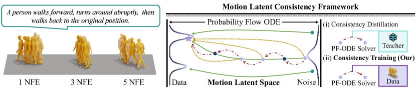
Figure 1: Our work achieves fewer NFE inferences via maintaining the consistency of the outputs of adjacent perturbed states on the precomputed PF-ODE trajectory. Following the consistency training pipeline, our approach is not limited by the additional pre-trained models required for consistency distillation when constructing trajectories. The color of humans darkens over time.

Upon the above limitations, we propose a Motion Latent Consistency Training (MLCT) framework for fast, high-fidelity, and text-matched motion generation. The first insight is to extend a motion autoencoder with the quantization constraint to extract low-dimension motion representations. It differs significantly from the widely-used variational representations in that the former are bounded finite states while the latter are unbounded continuous states. We restrict the representation boundaries with the hyperbolic tangent (Tanh) function and force the continuous representation to map to the nearest predefined clustering center. It allows flexibility in adjusting the upper limit of the latent space state to streamline the motion embedding space under inadequate training data. In addition, previous practice demonstrates that the boundedness of the representations contributes to sustaining stable inference in classifier-free guidance (CFG) techniques [18]. The second insight is to present a conditionally guided consistency training framework based on conditional trajectory simulation. The core insight is to consider ground truth motion representations as the simulation of a conditional initial state prediction and to replace the unconditional initial state estimation with an online updating unconditional consistency model based on additional loss items. Such a process without additional pre-training diffusion models, significantly improving the conditional generation performance.

We evaluate the proposed framework on two widely used datasets: KIT and HumanML. The results of our 1, 3, and 5 NFE generation are shown in Figure 1. Extensive experiments indicate the effectiveness of MLCT and its components. The proposed framework achieves state-of-the-art performance in motion generation in around few NFE ($\sim$14 ms).

To sum up, the contributions of this paper are as follows:

• We extend a flexible motion latent representation based on the quantization constraint, which are bounded finite states, providing a flexible and powerful latent space embedding scheme.

• We present the conditionally guided consistency training framework in latent representation space. To the best of our knowledge, we have explored consistency training in latent space for the first time, and are also the first to introduce CFG into consistency training.

• Our work achieves state-of-the-art results on two challenge datasets, saving over 80% of function evaluation iterations in latent space for real-time text-driven motion generation.

2 Related Work

Human motion generation. Human motion generation aims to synthesize human motion sequence under specified conditions, such as action categories [19, 20], audio [21, 22], and textual description [23, 2, 7]. Some multi-step generative methods have emerged recently with great success, such as auto-regressive [24, 25] and diffusion methods [1, 2, 7]. In particular, the latter is gradually dominating the research frontiers due to its stable distribution estimation capability and high-quality sampling results. Motiondiffuse [1] and MDM [2] were the pioneers in implementing diffusion frameworks for motion generation. MLD [7] realizes the latent space diffusion, which significantly improves the efficiency. M2DM [8] represents motion as discrete features and diffusion processes in finite state space with state-of-the-art performance. Some recent work [9] has focused on more controlled generation with equally excellent results. These works validate the outstanding capabilities of the motion diffusion framework and receive continuous attention.

Efficient diffusion sampling. Efficient diffusion sampling is the primary challenge of diffusion frameworks oriented to real-time generation tasks. Score-based method [11] relates the diffusion framework to a stochastic differential equation and notes that it has a special form known as the probability flow ODE. This is a milestone achievement. It guides the following works either to steer a simplified diffusion process through a specially designed form of ODE [26, 27, 14], or to skip a sufficiently large number of sampling steps via the more sophisticated ODE approximation solution strategy [12, 13]. While these works have proven effective in computer vision, they have received only finite reflections in motion diffusion frameworks. Previous state-of-the-art methods such as MLD [7] and GraphMotion [9] have utilized VAE-based representations and DDIM sampling strategies. These methods struggle to maintain generative performance with fewer NFE, and real-time inference remains challenging.

Consistency model. The consistency model [12] is a flexible diffusion sampling framework that allows the model to make trade-offs between fewer NFE and generation quality. Most studies [15, 16, 28, 29, 30, 31, 32] pile up on the application of consistency distillation in different tasks. Recent approaches [33, 32] have also investigated the application of Lora and control net to consistency modeling with impressive results. These methods rely on a strong teacher model as the distillation target, and training from scratch requires not only a large dataset support but also a lot of computational resources. ICM [17] further explores and improves consistency training methods to obtain similar performance to consistency distillation without pre-trained models. However, its lack of reflection on conditional PF-ODE trajectories limited its potential in the conditional diffusion framework. In addition, there is a gap in exploring consistency training frameworks in latent spaces. Upon the above limitation, our work focuses on building a latent consistency training framework with conditional PF-ODE trajectories simulation, which achieves few NFE and high-fidelity motion generation with minimal training cost.

3 Preliminaries

3.1 Score-based Diffusion Models

The diffusion model [34] i s a generative model that gradually injects Gaussian noise into the data and then generates samples from the noise through a reverse denoising process. Specifically, it gradually transforms the data distribution $p_{data}(x_{0})$ into a well-sampled prior distribution $p(x_{T})$ via a Gaussian perturbation kernel $p(x_{t}|x_{0})=\mathcal{N}(x_{t}|\alpha_{t}x_{0},\sigma_{t}^{2}I)$, where $\alpha_{t}$ and $\sigma_{t}$ are noise schedules. Recent studies have formalized it into a continuous time form, described as stochastic differential equations (SDEs),

$$dx_{t}=f(t)x_{t}dt+g(t)dw_{t},$$ (1)

where $t\in[\epsilon,T]$, $\epsilon$ and $T$ are the fixed positive constant, $w_{t}$ denotes the standard Brownian motion, $f$ and $g$ are the drift and diffusion coefficients respectively with follow from,

$$f(t)=\frac{d\log\alpha_{t}}{dt},\quad g^{2}(t)=\frac{d\sigma_{t}^{2}}{dt}-2\frac{d\log\alpha_{t}}{dt}\sigma_{t}^{2}.$$ (2)

Previous work has revealed that the reverse process of Equation 1 shares the same marginal probabilities with the probabilistic flow ODE:

$$dx_{t}=[f(t)x_{t}-\frac{1}{2}g^{2}(t)\nabla_{x_{t}}\log p(x_{t})]dt,$$ (3)

where $\nabla_{x}\log p(x_{t})$ is named the score function, which is the only unknown term in the sampling pipeline. An effective approach is training a time-dependent score network $\mathcal{S}_{\theta}(x_{t},t)$ to estimate $\nabla_{x}\log p(x_{t})$ based on conditional score matching, parameterized as the prediction of noise or initial value in forward diffusion. Further, Equation 3 can be solved in finite steps by numerical ODE solvers such as Euler [11] and Heun solvers [35]. Upon the above study, previous work also has explored conditional probabilities $p(x_{t}|y)$ for the more controlled generation, where $y$ is the condition such as text or action. One successful approach is known as Classifier-Free Guidance (CFG), which is parameterized as a linear combination of unconditional and conditional noise predictions, i.e. $\widetilde{z}_{\theta}(x_{t},t,c)=(1+\omega)z_{\theta}(x_{t},t,c)-\omega z_{\theta}(x_{t},t,\emptyset)$, where $\omega$ is guidance scale.

3.2 Consistency Models

Theoretically, the reverse process expressed by Equation 3 is deterministic, and the consistency model (CM) [14] achieves one-step or few-step generation by pulling in outputs on the same ODE trajectory. It is more formally expressed as,

$$\mathcal{S}_{\psi}(x_{t},t)\approx\mathcal{S}_{\psi}(x_{t^{\prime}},t^{\prime})\approx\mathcal{S}_{\psi}(x_{\epsilon},\epsilon)\quad\forall t,t^{\prime}\in[\epsilon,T],$$ (4)

which is known as the self-consistency property. To maintain the boundary conditions, existing consistency models are commonly parameterized by skip connections, i.e.,

$$\mathcal{S}_{\psi}(x_{t},t):=c_{skip}(t)x_{t}+c_{out}(t)\hat{\mathcal{S}}_{\psi}(x_{t},t)$$ (5)

where $c_{skip}(t)$ and $c_{out}(t)$ are differentiable functions satisfied $c_{skip}(\epsilon)=1$ and $c_{out}(\epsilon)=0$. For stabilize training, the consistency model maintaining target model $\mathcal{S}_{\psi}^{-}$, trained with the exponential moving average (EMA) of rate $\gamma$, that is $\psi^{-}\leftarrow\gamma\psi^{-}+(1-\gamma)\psi$. The consistency loss can be formulated as,

$$\mathcal{L}_{cm}(\psi,\psi^{-})=\mathbb{E}_{x,t}\big{[}d\big{(}\mathcal{S}_{\psi}(x_{t_{n+1}},t_{n+1}),\mathcal{S}_{\psi^{-}}(\hat{x}_{t_{n}},t_{n})\big{)}\big{]}$$ (6)

where $d(\cdot,\cdot)$ is a metric function such as mean square or pseudo-huber metric, and $\hat{x}_{t_{n}}$ is a one-step estimation from $x_{t_{n+1}}$ with ODE solvers applied in Equation 3.

4 Motion Latent Consistency Training

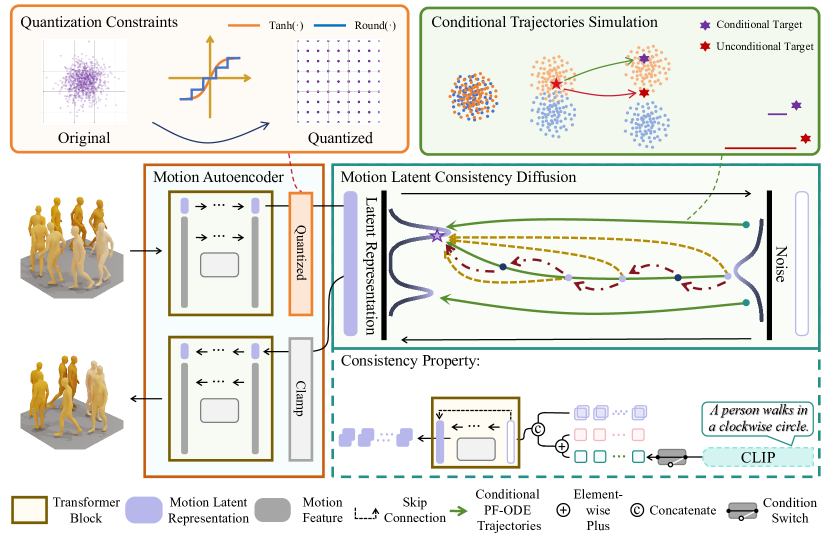
Figure 2: The overview of the proposed MLCT for fast, high-fidelity, and text-matched motion sequence generation. It consists of a motion autoencoder with the quantization constraint, which is used to learn various motion representations in low-dimensional, bounded and regularized latent spaces, and a motion consistency model that simulates conditional PF-ODE trajectories for capturing the corresponding motion latent presentation distributions and sampling with few NFE.

In this section, we focus on the conditional consistency training pipeline within motion latent representation. The overview of the proposed MLCT is shown in Figure 2.

4.1 Motion Latent Representation with the Quantization Constraint

We construct a motion autoencoder $\mathcal{G}=\{\mathcal{E},\mathcal{D}\}$ to realize encoding and reconstructing between motion sequences $x$ and motion latent representations $z$. Inspired by recent quantitative work [36] and the success of consistency training in raw pixel space, we utilize the quantization constraint to adjust the upper limit of motion state in the latent space and thus constrain the bounded and regularity of $z$. Specifically, each dimension of $z$ is sampled from a finite set $\mathcal{M}$ of size $2l+1$ as follow,

$$\mathcal{M}=\{z_{i};-1,-j/l,\cdots,0,\cdots,j/l,\cdots,1\}_{j=0}^{l}.$$ (7)

It is structurally analogous to the normalized raw pixel representation. Our work denotes $z\in\mathcal{R}^{n,d}$ as $n$ learnable tokens with $d$ dimension, aggregating the motion sequence features via attention computation [37]. We employ a hyperbolic tangent (tanh) function on the output of the encoder $\mathcal{E}$ to constrain the boundaries of the representation, and then quantize the result by a rounding operator $\mathcal{R}$. Furthermore, the gradient of quantized items is simulated by the previous state gradient to backpropagate the gradient normally, which is known as the straight-through estimator (STE) [38]. The motion latent representations $z_{m}$ are sampled by the following format,

$$z_{m}=\mathcal{R}\Big{(}l\cdot tanh(\mathcal{E}(x))\Big{)}/l.$$ (8)

The standard optimization target is to reconstruct motion information from $z$ with the decoder $\mathcal{D}$, i.e., to optimize the $l_{1}$ smooth error loss,

$$\mathcal{L}_{z}=\mathbb{E}_{x}\Big{[}d\Big{(}x,\mathcal{D}(z_{m})\Big{)}+\lambda_{j}d\Big{(}\mathcal{J}(x),\mathcal{J}(\mathcal{D}(z_{m}))\Big{)}\Big{]},$$ (9)

where $\mathcal{J}$ is a function to transform features such as joint rotations into joint coordinates, and it is also applied in MLD [7] and GraphMotion [9]. $\lambda_{j}$ is the balancing weight.

4.2 Conditionally Guided Consistency Training

For conditional motion generation, Class-Free Guidance (CFG) is crucial for synthesizing high-fidelity samples in most successful cases of motion diffusion models, such as MLD or GraphMotion. Previous work introduced CFG into the consistency distillation, demonstrating the feasibility of the consistency model on conditional PF-ODE trajectories. However, they rely on powerful pre-trained teacher models, which not only involve additional training costs but performance is limited by distillation errors. Therefore, we are motivated to simulate CFG more efficiently from the original motion latent representation following the consistency training framework to alleviate the computational burden.

The diffusion stage of MLCT begins with the variance preserving schedule [11] to perturbed motion latent representations $x_{\epsilon}=z$ with perturbation kernel $\mathcal{N}(x_{t};\alpha(t)x_{0},\sigma^{2}(t)I)$,

$$\alpha_{t}:=e^{-\frac{1}{4}t^{2}(\beta_{1}-\beta_{0})-\frac{1}{2}t\beta_{0}},\quad\sigma_{t}:=\sqrt{1-e^{2\alpha(t)}}.$$ (10)

The consistency model $\mathcal{S}_{\theta}$ has been constructed to predict $x_{\epsilon}$ from perturbed $x_{t}$ in a given PF-ODE trajectory. To maintain the boundary conditions that $\mathcal{S}_{\psi}(x_{\epsilon},\epsilon,c)=x_{\epsilon}$, we employ the same skip setting for Equation 5 as in LCM [15], which parameterized as follow:

$$\mathcal{S}_{\psi}(x_{t},t,c):=\frac{\eta^{2}}{(10t)^{2}+\eta^{2}}\cdot x_{t}+\frac{10t}{\sqrt{(10t)^{2}+\eta^{2}}}\cdot\widetilde{\mathcal{S}}_{\psi}(x_{t},t,c),$$ (11)

where $\widetilde{\mathcal{S}}_{\psi}$ is a transformer-based network and $\eta$ is a hyperparameter, which is usually set to 0.5. Following the self-consistency property (as detailed in Equation 4), the model $\mathcal{S}_{\psi}$ has to maintain the consistency of the output at the given perturbed state $x_{t}$ with the previous state $\widetilde{x}_{t-\Delta t}$ on the same ODE trajectory. The latter can be estimated via the DPM++ solver:

$$\widetilde{x}_{t-\Delta t}\approx\Phi(x_{\epsilon}^{\Phi},x_{t},x_{t-\Delta t})=\frac{\sigma_{t-\Delta t}}{\sigma_{t}}\cdot x_{t}-\alpha_{t-\Delta t}\cdot(e^{-h_{t}}-1)\cdot x_{\epsilon}^{\Phi},$$ (12)

where $h_{t}:=\lambda_{t-\Delta t}-\lambda_{t}$, $\lambda_{t}:=\log(\alpha_{t}/\sigma_{t})$, and $x_{\epsilon}^{\Phi}$ is the estimation of $x_{\epsilon}$ under the different sampling strategies. In particular, $x_{\epsilon}^{\Phi}$ can be parameterized as a linear combination of conditional and unconditional latent presentation prediction following the CFG strategy, i.e.,

$$x_{\epsilon}^{\Phi}(x_{t},t,c)=(1+\omega)\cdot\mathcal{F}_{\psi}(x_{t},t,c)-\omega\mathcal{F}_{\psi}(x_{t},t,\emptyset),$$ (13)

where $\mathcal{F}_{\psi}(\cdot)$ is well-trained and $x_{\epsilon}$-prediction-based motion diffusion model.

It is worth noting that $x_{\epsilon}$ can be utilized to simulate $\mathcal{F}_{\psi}(x_{t},t,c)$ as used in the vanilla consistency training pipeline. Furthermore, $\mathcal{F}_{\psi}(x_{t},t,\emptyset)$ can be replaced by $\mathcal{S}_{\psi}(x_{t},t,\emptyset)$ with online updating based on the additional unconditional loss item. Thus Equation 13 can be rewritten as:

$$x_{\epsilon}^{\Phi}(x_{t},t,c)=(1+\omega)\cdot x_{\epsilon}-\omega\mathcal{S}_{\psi}(x_{t},t,\emptyset).$$ (14)

We refer to Equation 14 as the conditional trajectory simulation. The optimization objective of the consistency model $\mathcal{S}_{\theta}$ is that,

$$\mathcal{L}_{c}=\mathbb{E}_{x,t}\Big{[}\underbrace{\frac{1}{\Delta t}d\Big{(}\mathcal{S}_{\psi}(x_{t},t,c),\mathcal{S}_{\psi^{-}}(\widetilde{x}_{t-\Delta t},t-\Delta t,c)\Big{)}}_{\text{Consistency Loss}}+\lambda_{c}\underbrace{d\Big{(}\mathcal{S}_{\psi}(x_{t},t,\emptyset),x_{\epsilon}\Big{)}}_{\text{Unconditional Loss}}\Big{]},$$ (15)

where $d(x,y)=\sqrt{(x-y)^{2}+\gamma^{2}}-\gamma$ is pseudo-huber metric, $\gamma$ is a constant, $\lambda_{c}$ is a balancing term. The target network $\mathcal{S}_{\psi^{-}}$ is updated after each iteration via EMA. More details of consistency training setting as well as training and inference pseudo-code are shown in the Appendix B.

5 Experiments

5.1 Experimental Setup

Datasets. We evaluate the proposed framework on two mainstream benchmarks for text-driven motion generation tasks, which are the KIT [39] and the HumanML3D [5]. The former contains 3,911 motions and their corresponding 6,363 natural language descriptions. The latter is a large 3D human motion dataset comprising the HumanAct12 [40] and AMASS [41] datasets, containing 14,616 motions and 44,970 descriptions.

Evaluation Metrics. Consistent with previous work, we evaluate the proposed framework in four parts. (a) Motion quality: we utilize the frechet inception distance (FID) to evaluate the distance in feature distribution between the generated data and the real data. (b) Condition matching: we first employ the R-precision to measure the correlation between the text description and the generated motion sequence and record the probability of the first $k=1,2,3$ matches. Then, we further calculate the distance between motions and texts by multi-modal distance (MM Dist). (c) Motion diversity: we compute differences between features with the diversity metric and then measure generative diversity in the same text input using multimodality (MM) metric. (d) Calculating burden: we first use the number of function evaluations (NFE) to evaluate the resource consumption required for inferring. We affirm that the NFE metric is only evaluated in this paper in the context of the reverse diffusion stage, as reported in LCM. Then, we further utilize the Average Inference Time per Sentence (AITS) measured in seconds to evaluate the inference efficiency of diffusion models.

Implementation Details. Our models are both transformer architectures with long skip connections [42]. Specifically, both the encoder $\mathcal{E}$ and decoder $\mathcal{D}$ contain 7 layers of transformer blocks with input dimensions 256, and each block contains 3 learnable tokens. The size of the finite set $\mathcal{M}$ is default setting as 2001, i.e. $l=1000$, and guidance scales $\omega$ default setting as 1 on HumanML3D and 2 on KIT. The consistency model $\mathcal{S}$ contains 11 layers of transformer blocks with input dimensions 512. The frozen CLIP-ViT-L-14 model [43] is used to be the text encoder. As shown in Figure 2, the text encoder encodes the text to a pooled output $p\in\mathcal{R}^{1,768}$ and then projects it as text embedding to sum with the time embedding before the input of each block. For the diffusion strategy 10, we follow the general settings of $\beta_{0}=0.002$ and $\beta_{1}=1$. All experiments except those specifically stated were configured by default to 5 NFE. For balance training, we set $\lambda_{j}$ as $10^{-3}$ and $\lambda_{c}$ as 1. All the proposed models are trained with the AdamW optimizer with a learning rate of $10^{-4}$.

Table 1: Comparisons to state-of-the-art methods on the HumanML test set. We repeat all the evaluations 20 times and report the average with a 95% confidence interval. "$\uparrow$" denotes that higher is better. "$\downarrow$" denotes that lower is better. "$\rightarrow$" denotes that results are better if the metric is closer to the real motion. ${\dagger}$ denotes that classifier-free guidance is utilized, causing a double inference burden in each NFE. Bold and underlined indicate the best and second-best results, respectively. The gray background color indicates the default configuration.

Method	R-Precision $\uparrow$			FID $\downarrow$	MM-Dist$\downarrow$	Diversity$\rightarrow$	MModality$\uparrow$	NFE$\downarrow$
	Top-1	Top-2	Top-3
Real	$0.511^{\pm.003}$	$0.703^{\pm.003}$	$0.797^{\pm.002}$	$0.002^{\pm.000}$	$2.974^{\pm.008}$	$9.503^{\pm.065}$	-	-
T2M[5]	$0.457^{\pm.002}$	$0.639^{\pm.003}$	$0.740^{\pm.003}$	$1.067^{\pm.002}$	$3.340^{\pm.008}$	$9.188^{\pm.002}$	$2.090^{\pm.083}$	-
MDM [2]	$0.320^{\pm.005}$	$0.498^{\pm.004}$	$0.611^{\pm.007}$	$0.544^{\pm.044}$	$\underline{5.566}^{\pm.027}$	$\underline{9.559}^{\pm.086}$	$2.799^{\pm.072}$	1000
MotionDiffuse [1]	$0.491^{\pm.001}$	$0.681^{\pm.001}$	$\underline{0.782}^{\pm.001}$	$0.630^{\pm.001}$	$\underline{3.113}^{\pm.001}$	$9.410^{\pm.049}$	$1.553^{\pm.042}$	1000
MLD† [7]	$0.481^{\pm.003}$	$0.673^{\pm.003}$	$0.772^{\pm.002}$	$0.473^{\pm.013}$	$3.196^{\pm.010}$	$9.724^{\pm.082}$	$2.413^{\pm.079}$	50
GraphMotion†[9]	$\textbf{0.504}^{\pm.003}$	$\textbf{0.699}^{\pm.002}$	$\textbf{0.785}^{\pm.002}$	$\underline{0.116}^{\pm.007}$	$\textbf{3.070}^{\pm.008}$	$9.692^{\pm.067}$	$2.766^{\pm.096}$	150
T2M-GPT [24]	$0.491^{\pm.003}$	$0.680^{\pm.003}$	$0.775^{\pm.002}$	$\underline{0.116}^{\pm.004}$	$3.118^{\pm.011}$	$9.761^{\pm.081}$	$1.856^{\pm.011}$	51
M2DM [8]	$\underline{0.497}^{\pm.003}$	$\underline{0.682}^{\pm.002}$	$0.763^{\pm.003}$	$0.352^{\pm.005}$	$3.134^{\pm.010}$	$9.926^{\pm.073}$	$\textbf{3.587}^{\pm.072}$	100
Our	$0.483^{\pm.002}$	$0.676^{\pm.002}$	$0.775^{\pm.002}$	$0.143^{\pm.005}$	$3.133^{\pm.009}$	$9.613^{\pm.082}$	$2.872^{\pm.072}$	5
Our	$0.484^{\pm.003}$	$0.672^{\pm.002}$	$0.771^{\pm.002}$	$\textbf{0.114}^{\pm.005}$	$3.133^{\pm.009}$	$\textbf{9.507}^{\pm.085}$	$\underline{2.982}^{\pm.066}$	10

Table 2: Comparisons to state-of-the-art methods on the KIT test set. Marker meaning is consistent with Table 1.

Method	R-Precision $\uparrow$			FID $\downarrow$	MM-Dist$\downarrow$	Diversity$\rightarrow$	MModality$\uparrow$	NFE$\downarrow$
	Top-1	Top-2	Top-3
Real	$0.424^{\pm.005}$	$0.649^{\pm.006}$	$0.779^{\pm.006}$	$0.031^{\pm.004}$	$2.788^{\pm.012}$	$11.08^{\pm.097}$	-	-
T2M[5]	$0.370^{\pm.005}$	$0.569^{\pm.007}$	$0.693^{\pm.007}$	$2.770^{\pm.109}$	$3.401^{\pm.008}$	$10.91^{\pm.119}$	$1.482^{\pm.065}$	-
MDM [2]	$0.164^{\pm.004}$	$0.291^{\pm.004}$	$0.396^{\pm.004}$	$0.497^{\pm.021}$	$9.191^{\pm.022}$	$10.85^{\pm.109}$	$1.907^{\pm.214}$	1000
MotionDiffuse [1]	$0.417^{\pm.004}$	$0.621^{\pm.004}$	$0.739^{\pm.004}$	$1.954^{\pm.062}$	$2.958^{\pm.005}$	$\textbf{11.10}^{\pm.143}$	$0.730^{\pm.013}$	1000
MLD† [7]	$0.390^{\pm.008}$	$0.609^{\pm.008}$	$0.734^{\pm.007}$	$0.404^{\pm.027}$	$3.204^{\pm.027}$	$10.80^{\pm.117}$	$2.192^{\pm.071}$	50
GraphMotion †[9]	$0.429^{\pm.007}$	$0.648^{\pm.006}$	$\underline{0.769}^{\pm.006}$	$\textbf{0.313}^{\pm.013}$	$3.076^{\pm.022}$	$11.12^{\pm.135}$	$\textbf{3.627}^{\pm.113}$	150
T2M-GPT [24]	$0.416^{\pm.006}$	$0.627^{\pm.006}$	$0.745^{\pm.006}$	$0.514^{\pm.029}$	$3.007^{\pm.023}$	$10.921^{\pm.108}$	$1.570^{\pm.0.39}$	51
M2DM [8]	$0.416^{\pm.004}$	$0.628^{\pm.004}$	$0.743^{\pm.004}$	$0.515^{\pm.029}$	$3.015^{\pm.017}$	$11.417^{\pm.970}$	$\underline{3.325}^{\pm.370}$	100
Our	$\textbf{0.450}^{\pm.007}$	$\underline{0.660}^{\pm.005}$	$\textbf{0.785}^{\pm.005}$	$\underline{0.321}^{\pm.015}$	$\textbf{2.765}^{\pm.018}$	$11.045^{\pm.121}$	$1.353^{\pm.028}$	5
Our	$\underline{0.444}^{\pm.005}$	$\textbf{0.665}^{\pm.006}$	$\textbf{0.785}^{\pm.004}$	$0.341^{\pm.013}$	$\underline{2.768}^{\pm.020}$	$\underline{11.044}^{\pm.123}$	$1.327^{\pm.029}$	10

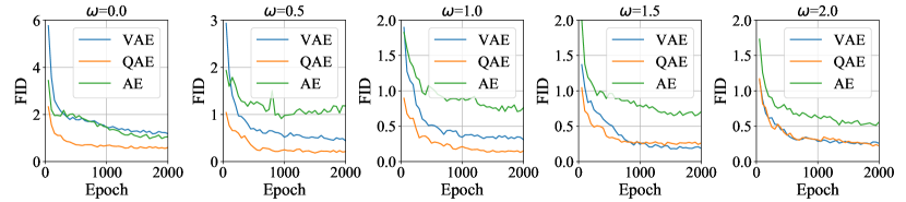
Figure 3: Ablation study of the quantized autoencoder employed in our framework with the conventional variational autoencoder and the vanilla autoencoder under different guidance scales on the HumanML test set. We repeat all evaluations 3 times at each 50 epoch and report the average values.

Table 3: Ablation study of our framework with more generation metrics under different guidance parameters on the HumanML3D test set. Marker meaning is consistent with Table 1.

$\omega$	R-Precision $\uparrow$			FID $\downarrow$	MM-Dist$\downarrow$	Diversity$\rightarrow$	MModality$\uparrow$
	Top-1	Top-2	Top-3
Real	$0.511^{\pm.003}$	$0.703^{\pm.003}$	$0.797^{\pm.002}$	$0.002^{\pm.000}$	$2.974^{\pm.008}$	$9.503^{\pm.065}$	-
0	$0.410^{\pm.002}$	$0.595^{\pm.003}$	$0.705^{\pm.003}$	$0.582^{\pm.015}$	$3.546^{\pm.009}$	$9.171^{\pm.067}$	$\textbf{3.959}^{\pm.085}$
0.5	$0.464^{\pm.002}$	$\underline{0.676}^{\pm.002}$	$\underline{0.775}^{\pm.002}$	$\underline{0.217}^{\pm.008}$	$3.244^{\pm.009}$	$\textbf{9.447}^{\pm.069}$	$\underline{3.396}^{\pm.078}$
1	$\textbf{0.484}^{\pm.002}$	$\underline{0.676}^{\pm.002}$	$\underline{0.775}^{\pm.002}$	$\textbf{0.143}^{\pm.005}$	$\textbf{3.133}^{\pm.009}$	$\underline{9.613}^{\pm.082}$	$2.872^{\pm.072}$
1.5	$\underline{0.479}^{\pm.004}$	$0.673^{\pm.004}$	$0.774^{\pm.003}$	$0.249^{\pm.008}$	$3.171^{\pm.010}$	$9.802^{\pm.089}$	$2.458^{\pm.059}$
2	$\textbf{0.484}^{\pm.002}$	$\textbf{0.677}^{\pm.003}$	$\textbf{0.776}^{\pm.002}$	$0.268^{\pm.008}$	$\underline{3.167}^{\pm.007}$	$9.889^{\pm.083}$	$2.231^{\pm.040}$

Table 4: Ablation study of different number of token on the HumanML3D test set. Marker meaning is consistent with Table 1.

Token	R-Precision Top-3$\uparrow$	FID $\downarrow$	MModality $\uparrow$
2	$0.772^{\pm.002}$	$0.247^{\pm.009}$	$\underline{2.935}^{\pm.073}$
3	$0.775^{\pm.003}$	$\textbf{0.143}^{\pm.005}$	$2.872^{\pm.072}$
4	$\underline{0.780}^{\pm.003}$	$0.218^{\pm.005}$	$2.828^{\pm.053}$
5	$\textbf{0.781}^{\pm.002}$	$\underline{0.204}^{\pm.007}$	$2.812^{\pm.061}$
6	$0.775^{\pm.002}$	$0.222^{\pm.010}$	$\textbf{2.986}^{\pm.067}$

Table 5: Ablation study of different sizes of representation finite set on the HumanML3D test set. Marker meaning is consistent with Table 1.

$l$	R-Precision Top-3 $\uparrow$	FID $\downarrow$	MModality $\uparrow$
100	$\underline{0.779}^{\pm.002}$	$0.224^{\pm.008}$	$2.764^{\pm.056}$
500	$0.776^{\pm.002}$	$0.190^{\pm.006}$	$2.995^{\pm.064}$
1000	$0.775^{\pm.003}$	$\textbf{0.143}^{\pm.005}$	$2.872^{\pm.072}$
1500	$0.775^{\pm.002}$	$0.208^{\pm.007}$	$2.848^{\pm.066}$
2000	$\textbf{0.780}^{\pm.002}$	$\underline{0.157}^{\pm.006}$	$\underline{2.878}^{\pm.065}$

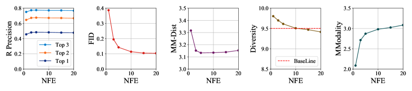
Figure 4: Comparison of generation performance under few NFE on the HumanML3D test set. Our model achieves the trade-off between generation performance and inference cost in around 5 NFE.

5.2 Comparisons to State-of-the-art Methods

The test results of HumanML and KIT are shown in Table 1 and Table 2, respectively. Our framework achieves state-of-the-art generation performance. Compared to existing motion diffusion generation frameworks with more than 50-1000 iterations (e.g., MDM, MotionDiffuse, and MLD), our approach reduces the computational burden by over tenfold without severely degrading the generation quality (the FID metric under 5 NFE of 0.143 vs. 0.116 for GraphMotion and T2M-GPT). With the payment of additional computational effort, our FID metric can be further reduced to 0.144 under 10 NFE. In addition, we observed remarkably controllable and excellent generation quality on datasets with limited data amounts such as KIT. Remarkably, our inference pipeline is without additional text preprocessing as used in GraphMotion. Sampling in fewer steps also has not significantly reduced diversity and multi-modality metrics on HumanML3D, which remain competitive. Our proposed framework achieves an optimal trade-off between controllability, generation quality, diversity, and inference efficiency.

5.3 Ablation Study

Effectiveness of each component. We explore the generative performance of the classifier-free guidance and the results are reported in Figure 3. For the control group, we set up two widespread motion latent representations: the first is the variational latent representation with KL constraints, and the second is the vanilla latent representation without any regularity constraint. Both of them are unbounded continuous representations. When the guidance scale $\omega$ equals 0, the model degenerates into a vanilla consistency model. We discover that various levels of classifier-free guidance contribute to significantly improving the generation quality under each representation even if the scale is small enough. There is no significant difference between vanilla representations and variational representations in the vanilla consistency training, but the irregular nature under the conditionally guided strategy is detrimental to generative performance. Our proposed latent representations based on quantization constraints are bounded and succinct and show stronger performance advantages over variational representations. In more detail, we discuss more comprehensive generation metrics at different guidance parameters and the results are reported in Table 3. The optimal generation performance is achieved when $\omega$ reaches 1. As the guidance parameters increase, controllability gradually improves, with a corresponding decrease in diversity.

Ablation study on the different model hyperparameters. In Table 5 and Table 5, we test the model performance with different hyperparameters. Consistent with the findings of MLD, increasing the number of tokens does not remarkably increase the generation quality. Appropriately increasing the size of the finite set $2l+1$ is beneficial in improving the generation results.

Ablation study on the different sampling steps. The results at different sampling steps are shown in Figure 4. As the NFE increases, there is a corresponding increase in generation quality and diversity. The two main controllability metrics peak at around 5 NFEs, followed by a slow decline.

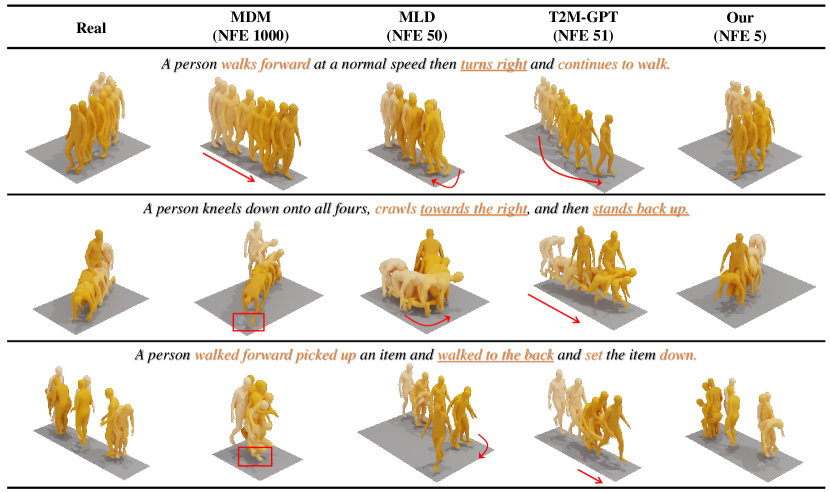
Figure 5: Qualitative analysis of our model and previous models. We provide three textual prompts for the motion visualization results. We achieve better motion generation performance to match some text conditions with fewer NFE.

Table 6: Comparison of Average Inference Time per Sentence (AITS) with previous SOTA models on single RTX 4090 GPU. We repeat the evaluations 100 times and report the average metric.

Method	MDM	MotionDiffuse	MLD	T2M-GPT	GraphMotion	Our (3 NFE)	Our (5 NFE)	Our (10 NFE)
AITS (s)	7.5604	5.8745	0.0786	0.2168	0.5417	0.0104	0.0148	0.0247

5.4 Time Cost and Qualitative Results

For the HumanML dataset, our motion autoencoder and consistency model were trained on an RTX 4090 GPU for 1500 and 2000 epochs, in about 12 and 15 hours, respectively. The training configurations are consistent on the KIT dataset and only require 2 and 2.5 hours. Figure 5 and Table 6 show the comparison of the qualitative results and the average inference time with the previous model, respectively. We achieve better text-matching capabilities while saving over 80% inference time than the existing fastest model. In particular, we reduce over 95% of the inference cost for the same FID compared to GraphMotion (the FID metric under 10 NFE of 0.114 vs. 0.116 for GraphMotion).

6 Conclusion

In this paper, we propose a motion latent consistency training framework, called MLCT, for fast, high-fidelity, and text-matched motion generation. It encodes motion sequences of arbitrary length into representational tokens with the quantization constraint and constrains the consistency of outputs on the same conditional PF-ODE trajectory with minimal training costs. Our model and each of its components have been validated through extensive experiments and achieve the best trade-off between performance and computational burden in few NFE. Our approach can provide a reference for subsequent latent consistency model training for different tasks.

This appendix provides additional discussions (Section A), more implementation details (Section B), additional ablation study (Section C), more qualitative results (Section D), user study (Section E), and details of evaluation metric (Section F).

Code. Our code will soon be open source.

Appendix A Additional Discussions

A.1 Potential Negative Societal Impacts

Our work enhances the efficiency of human motion synthesis and may be applied to generate fake information, which may threaten information security and intellectual property rights. In embodied intelligence, it may generate irrational robot joint mappings, which may cause property damage and security risks.

A.2 Limitation

Our work still has some directions for improvement: (i) The MLCT follows the diffusion modeling framework, and its stochastic nature favors diversity, but may sometimes produce undesired results. (ii) We aim at efficient motion generation and lack a discussion on fine-grained motion control. Fortunately, our proposed method is a generalized diffusion model training framework with fewer NFE. Some recent common textual controllers (such as GraphMotion) can be integrated into our work. (iii) Our set of textual instructions focuses on the annotated data of HumanML3D, but it may be limited, and out-of-domain instructions may occur resulting in unreasonable sample generation. This concern also arises in previous work such as GraphMotion or MLD.

A.3 Future Work

We would like to include more physical constraints in our follow-up work to minimize undesired motion generation and adopt a more appropriate text extractor for fine-grained motion control. Noting the rise of large language models, subsequent works could utilize them to assist in understanding a broader context of semantic instructions. In addition, zero-shot editing for consistency training based on large language models is also worthy of research.

Input: Train set $\Gamma=\{(x^{(n)},c^{(n)})\}^{N}_{n=1}$, Motion AutoEncoder $\mathcal{G}=\{\mathcal{E},\mathcal{D}\}$ with initial parameter $\theta$, size $2l+1$ of finite set $\mathcal{M}$, Joint Transform Function $\mathcal{J}$, Motion Consistency Model $\mathcal{S}$ with initial parameter $\psi$ and $\psi^{-}$, ODE Solver $\Phi$, Timestep Scheduler $\{t_{i}\}_{i=0}^{I}$, Guidance Scale $\omega$, Learning Ratio $\eta$, EMA Ratio $\gamma$, Balance Weight $\lambda_{j}$ and $\lambda_{c}$;

1

2# Stage 1: Motion AutoEncoder Training.

3repeat

4       Sample motion $x\sim\Gamma$;

      $z_{e}\leftarrow\mathcal{E}(x)$;

        // Motion Encoding.

5      

      $z_{m}\leftarrow\mathcal{R}\Big{(}l\cdot tanh(z_{e})\Big{)}/l$;

        // Quantization Constraint.$\mathcal{R}$ denotes Rounding Operator.

6      

      $\mathcal{L}_{z}\leftarrow\mathbb{E}_{x}\Big{[}d\Big{(}x,\mathcal{D}(z_{m})\Big{)}+\lambda_{j}d\Big{(}\mathcal{J}(x),\mathcal{J}(\mathcal{D}(z_{m}))\Big{)}\Big{]}$;

        // Loss.

7      

      $\theta\leftarrow\theta-\eta\nabla_{\theta}\mathcal{L}_{z}$.

        // Update $\theta$.

8      

9until convergence

10# Stage 2: Motion Consistency Training.

11repeat

12       Sample motion $x$ and condition $c\sim\Gamma$, noise $z\sim\mathcal{N}(0,I)$, timestep $t_{i},t_{i-1}\sim\{t_{i}\}_{i=0}^{I}$;

      $x_{\epsilon}\leftarrow\mathcal{R}\Big{(}l\cdot tanh(\mathcal{E}(x))\Big{)}/l$;

        // Motion Encoding with the Quantization Constraint.

13      

      $x_{t_{i}}\leftarrow\alpha_{t_{i}}\cdot x_{\epsilon}+\sigma_{t_{i}}\cdot z$;

        // Perturbed Data. $\alpha_{t}$ and $\sigma_{t}$ Detailed in Equation 10.

14      

      $x_{\epsilon}^{\Phi}\leftarrow(1+\omega)\cdot x_{\epsilon}-\omega\mathcal{S}_{\psi}(x_{t_{i}},t_{i},\emptyset);$

        // CFG in Consistency Training.

15      

      $x_{\epsilon}^{\Phi}\leftarrow\text{clamp}(x_{\epsilon}^{\Phi},-1,1);$

        // Clamp.

16      

      $\widetilde{x}_{t_{i-1}}\leftarrow\Phi(x_{\epsilon}^{\Phi},t_{i},t_{i-1})$;

        // One-step Numerical Estimation with Equation 12.

17      

      $\mathcal{L}_{c}\leftarrow\mathbb{E}_{x,t}\Big{[}\frac{1}{t_{i}-t_{i-1}}d\Big{(}\mathcal{S}_{\psi}(x_{t_{i}},t_{i},c),\mathcal{S}_{\psi^{-}}(\widetilde{x}_{t_{i-1}},t_{i-1},c)\Big{)}+\lambda_{c}d\Big{(}\mathcal{S}_{\psi}(x_{t_{i}},t_{i},\emptyset),x_{\epsilon}\Big{)}\Big{]}$;

        // Loss.

18      

      $\psi\leftarrow\psi-\eta\nabla_{\psi}\mathcal{L}_{c}$;

        // Update $\psi$.

19      

      $\psi^{-}\leftarrow\text{stopgrad}(\gamma\psi^{-}+(1-\gamma)\psi).$

        // Update $\psi^{-}$.

20      

21until convergence

Algorithm 1 Motion Latent Consistency Training.

Appendix B More Implementation Details

For diffusion time horizon $[\epsilon,T]$ into $N-1$ sub-intervals, we set $\epsilon$ is 0.002, $T$ is 1, $N$ is 50. We follow the consistency model [14] to determine $t_{i}=(\epsilon^{1/\rho}+\frac{i-1}{N-1}(T^{1/\rho}-\epsilon^{1/\rho}))^{\rho}$, where $\rho=2$. In addition, we set the EMA rate to $\gamma=0.995$ in all experiments. For better reproducibility, we provide pseudo-code for training and inference, as shown in Algorithm 1 and Algorithm 2, respectively.

Input: Motion AutoEncoder $\mathcal{G}=\{\mathcal{E},\mathcal{D}\}$, Joint Transform Function $\mathcal{J}$, Motion Consistency Model $\mathcal{S}$, Condition $c$, Max Number of Function Evaluations $N$, Timestep Scheduler $\{t_{i}\}_{i=0}^{N}$;

Result: Motion Sequence $x$.

1

2Sample $x_{t_{N}},z\sim\mathcal{N}(0,I)$;

3for i=N to 1 do

4       if i != N then

             $x_{t_{i}}\leftarrow\alpha_{t_{i}}\cdot x_{\epsilon}+\sigma_{t_{i}}\cdot z$;

              // Perturbed Data.

5            

      $x_{\epsilon}^{pred}\leftarrow\mathcal{S}_{\psi}(x_{t_{i}},t_{i},c)$;

        // Denoising.

6      

      $x_{\epsilon}^{pred}\leftarrow\text{clamp}(x_{\epsilon}^{pred},-1,1)$;

        // Clamp.

7      

$x=\mathcal{D}(x_{t})$.

  // Motion Decoding.

Algorithm 2 Motion Latent Consistency Inferring.

Appendix C Additional Ablation Study

Table 7: Ablation study of more different guidance scales on two challenging benchmark. Marker meaning is consistent with Table 1.

Dataset	$\omega$	R-Precision $\uparrow$			FID $\downarrow$	MM-Dist $\downarrow$	Diversity $\rightarrow$	MModality $\uparrow$
		Top-1	Top-2	Top-3
HumanML	Real	$0.511^{\pm.003}$	$0.703^{\pm.003}$	$0.797^{\pm.002}$	$0.002^{\pm.000}$	$2.974^{\pm.008}$	$9.503^{\pm.065}$	-
	0	$0.410^{\pm.002}$	$0.595^{\pm.003}$	$0.705^{\pm.003}$	$0.582^{\pm.015}$	$3.546^{\pm.009}$	$9.171^{\pm.067}$	$\textbf{3.959}^{\pm.085}$
	1	$\textbf{0.484}^{\pm.002}$	$\underline{0.676}^{\pm.002}$	$\underline{0.775}^{\pm.002}$	$\textbf{0.143}^{\pm.005}$	$\textbf{3.133}^{\pm.009}$	$\underline{9.613}^{\pm.082}$	$\underline{2.872}^{\pm.072}$
	2	$\textbf{0.484}^{\pm.002}$	$\textbf{0.677}^{\pm.003}$	$\textbf{0.776}^{\pm.002}$	$0.268^{\pm.008}$	$3.167^{\pm.007}$	$9.889^{\pm.083}$	$2.231^{\pm.040}$
	3	$\textbf{0.484}^{\pm.002}$	$\underline{0.676}^{\pm.001}$	$\underline{0.775}^{\pm.002}$	$\underline{0.171}^{\pm.005}$	$\underline{3.134}^{\pm.007}$	$9.790^{\pm.088}$	$2.169^{\pm.048}$
	4	$0.476^{\pm.002}$	$0.671^{\pm.002}$	$0.770^{\pm.002}$	$0.284^{\pm.006}$	$3.199^{\pm.010}$	$9.929^{\pm.083}$	$2.073^{\pm.046}$
	5	$\underline{0.477}^{\pm.002}$	$0.669^{\pm.002}$	$0.769^{\pm.002}$	$0.279^{\pm.005}$	$3.192^{\pm.009}$	$\textbf{9.493}^{\pm.083}$	$2.080^{\pm.054}$
	6	$\underline{0.477}^{\pm.002}$	$0.667^{\pm.002}$	$0.767^{\pm.002}$	$0.215^{\pm.004}$	$3.197^{\pm.008}$	$9.777^{\pm.004}$	$2.019^{\pm.040}$
	7	$0.421^{\pm.003}$	$0.613^{\pm.003}$	$0.720^{\pm.002}$	$0.485^{\pm.012}$	$3.587^{\pm.010}$	$9.771^{\pm.083}$	$1.519^{\pm.036}$
KIT	Real	$0.424^{\pm.005}$	$0.649^{\pm.006}$	$0.779^{\pm.006}$	$0.031^{\pm.004}$	$2.788^{\pm.012}$	$11.08^{\pm.097}$	-
	0	$0.414^{\pm.007}$	$0.632^{\pm.006}$	$0.775^{\pm.005}$	$0.585^{\pm.027}$	$2.996^{\pm.048}$	$\textbf{10.967}^{\pm.111}$	$\textbf{2.106}^{\pm.048}$
	1	$0.439^{\pm.005}$	$0.662^{\pm.007}$	$0.783^{\pm.005}$	$0.373^{\pm.016}$	$2.766^{\pm.018}$	$11.084^{\pm.106}$	$\underline{1.511}^{\pm.028}$
	2	$\textbf{0.450}^{\pm.007}$	$0.660^{\pm.005}$	$0.785^{\pm.005}$	$\textbf{0.321}^{\pm.015}$	$2.765^{\pm.018}$	$11.045^{\pm.121}$	$1.353^{\pm.028}$
	3	$\underline{0.449}^{\pm.006}$	$\underline{0.665}^{\pm.006}$	$\underline{0.788}^{\pm.004}$	$\underline{0.366}^{\pm.014}$	$\underline{2.761}^{\pm.021}$	$11.002^{\pm.112}$	$1.359^{\pm.035}$
	4	$0.445^{\pm.007}$	$\textbf{0.672}^{\pm.004}$	$\textbf{0.789}^{\pm.005}$	$0.403^{\pm.020}$	$\textbf{2.756}^{\pm.018}$	$\textbf{10.967}^{\pm.074}$	$1.324^{\pm.031}$
	5	$0.440^{\pm.005}$	$0.663^{\pm.005}$	$0.785^{\pm.003}$	$0.445^{\pm.016}$	$2.804^{\pm.020}$	$11.033^{\pm.114}$	$1.167^{\pm.027}$
	6	$0.443^{\pm.005}$	$0.662^{\pm.005}$	$0.786^{\pm.004}$	$0.503^{\pm.021}$	$2.789^{\pm.017}$	$11.002^{\pm.118}$	$1.183^{\pm.026}$
	7	$0.437^{\pm.006}$	$0.656^{\pm.005}$	$0.781^{\pm.004}$	$0.509^{\pm.002}$	$2.797^{\pm.017}$	$\underline{10.976}^{\pm.112}$	$1.248^{\pm.035}$

Additional ablation study on guidance scales. We note that previous diffusion models can usually be set up with large CFG guidance scales (typically up to 7.5). Therefore, we show ablation experiments with more guidance scales, and the results are reported in Table 7. The results with the introduction of conditional guidance all outperform the vanilla consistency training. The optimal configuration focuses on $\omega$ equal to 1 to 3, while larger guidance scales will compromise the quality of generation. Larger guidance scales may lead to unexpected results, while the clamp operator, which is designed to make training stable, enforces constraints on the boundaries, which in turn introduces numerical errors leading to poorer results.

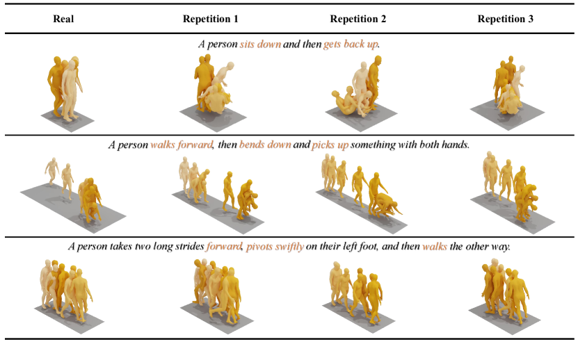
Figure 6: Qualitative analysis of the diversity. Our MLCT can generate diverse samples based on given textual prompts.

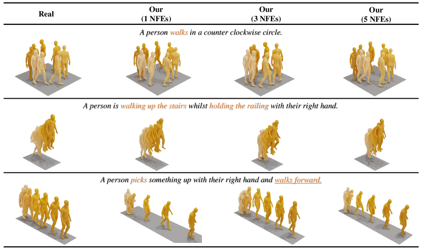
Figure 7: Qualitative analysis of few NFE inference. Our MLCT allows the generation of high-quality samples in extremely few iterations.

Appendix D More Qualitative Results

Diversity. We provide visualization results for multiple motion sequences generated from the same text prompt, as shown in Figure 6. It validates the potential of MLCT for diverse motion generation.

Few NFE inference. We show the qualitative results under few NFE inference in Figure 7. In most cases, our model requires only 1 function evaluation to generate the desired motion sequences. Moreover, the details will be refined as the amount of computation increases.

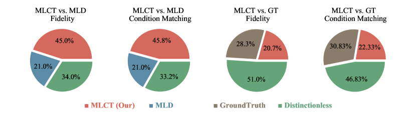
Figure 8: User studies for quantitative comparison. We follow MLD [7] that utilize the force-choice paradigm to ask "which of the two motions is more realistic?" and "which of the two motions corresponds better to the text prompt?" We show the preference rate of MLCT over the MLD and Ground Truth data.

Appendix E User Study

Following the configuration in MLD, we set up UserStudy. We randomly generated 30 sets of text descriptions in the test set of the HumanML3D dataset and used MLCT and MLD to generate the corresponding text, respectively. We invited 20 participants to provide two comparisons: the MLCT and the MLD, and the MLCT and the ground truth motion in the dataset. Each set of motions will be compared for fidelity and condition matching. The results are reported in Figure 8. Our method outperforms MLD with a low inference cost of 5 NFE and is even competitive with ground truth results provided by motion capture devices in terms of fidelity and condition matching.

Appendix F Details of Evaluation Metric

We utilize the standard feature extractor [5] to calculate the features of motions and texts. The parameters of metrics are consistent with previous work [7, 9].

Frechet Inception Distance (FID). FID is the principal metric to evaluate the generation quality, which examines the similarity between the generated motion distribution and the ground truth motion distribution. It is formalized as:

$$\text{FID}=\|\mu_{gt}-\mu_{gen}\|^{2}+\text{Tr}(\Sigma_{gt}+\Sigma_{gen}-2(\Sigma_{gt}\cdot\Sigma_{gen})^{\frac{1}{2}}),$$ (16)

where $\mu$ and $\Sigma$ denote the mean and the covariance matrix of motion features, and Tr denotes the trace of the corresponding matrix.

R-Precision. Given a motion feature and 32 textual descriptions (one of ground truth and the others are randomly selected mismatched descriptions), we calculate the matching accuracy of text and motion for Top 1/2/3.

Multimodal Distance (MM-Dist). For $N$ randomly generated motions, we calculate the average Euclidean distances between motion features and text features. It is formalized as:

$$\text{MM-Dist}=\dfrac{1}{N}\sum_{i=1}^{N}\|f_{m,i}-f_{t,i}\|,$$ (17)

where $f_{m,i}$ and $f_{t,i}$ denote the feature of $i$-th motion and text.

Diversity. We calculate the average Euclidean distances between two randomly divided groups of generated motion features $\{x\}_{i=1}^{N}$ and $\{x^{\prime}\}_{i=1}^{N}$. It is formalized as:

$$\text{Diversity}=\dfrac{1}{N}\sum_{i=1}^{N}\|x_{i}-x_{i}^{\prime}\|.$$ (18)

Multimodality (MModality). For $J$ text descriptions, we are randomly sampled two subsets of same size $N$ from all motions generated by $j$-th text descriptions, with motion features $\{x_{j,1},\cdots,x_{j,N}\}$ and $\{x_{j,1}^{\prime},\cdots,x_{j,N}^{\prime}\}$. We calculate the average Euclidean distance formalized as:

$$\text{MModality}=\dfrac{1}{J\times N}\sum_{j=1}^{J}\sum_{n=1}^{N}\|x_{j,n}-x_{j,n}^{\prime}\|.$$ (19)

Average Inference Time per Sentence (AITS). We repeatedly testing $N$ times for generating the longest motion, and report the average inference time.

The Number of Function Evaluation (NFE). We report the number of iterations in the reverse diffusion process.

References

- [1] Mingyuan Zhang, Zhongang Cai, Liang Pan, Fangzhou Hong, Xinying Guo, Lei Yang, and Ziwei Liu. Motiondiffuse: Text-driven human motion generation with diffusion model. arXiv preprint arXiv:2208.15001, 2022.
- [2] Guy Tevet, Sigal Raab, Brian Gordon, Yonatan Shafir, Daniel Cohen-Or, and Amit H Bermano. Human motion diffusion model. In International Conference on Learning Representations, 2023.
- [3] Mingyuan Zhang, Xinying Guo, Liang Pan, Zhongang Cai, Fangzhou Hong, Huirong Li, Lei Yang, and Ziwei Liu. Remodiffuse: Retrieval-augmented motion diffusion model. In Proceedings of the IEEE/CVF International Conference on Computer Vision (ICCV), pages 364–373, October 2023.
- [4] Haoye Cai, Chunyan Bai, Yu-Wing Tai, and Chi-Keung Tang. Deep video generation, prediction and completion of human action sequences. In Proceedings of the European conference on computer vision (ECCV), pages 366–382, 2018.
- [5] Chuan Guo, Shihao Zou, Xinxin Zuo, Sen Wang, Wei Ji, Xingyu Li, and Li Cheng. Generating diverse and natural 3d human motions from text. In Proceedings of the IEEE/CVF Conference on Computer Vision and Pattern Recognition, pages 5152–5161, 2022.
- [6] Mathis Petrovich, Michael J Black, and Gül Varol. Temos: Generating diverse human motions from textual descriptions. In European Conference on Computer Vision, pages 480–497. Springer, 2022.
- [7] Xin Chen, Biao Jiang, Wen Liu, Zilong Huang, Bin Fu, Tao Chen, and Gang Yu. Executing your commands via motion diffusion in latent space. In Proceedings of the IEEE/CVF Conference on Computer Vision and Pattern Recognition, pages 18000–18010, 2023.
- [8] Hanyang Kong, Kehong Gong, Dongze Lian, Michael Bi Mi, and Xinchao Wang. Priority-centric human motion generation in discrete latent space. In Proceedings of the IEEE/CVF International Conference on Computer Vision, pages 14806–14816, 2023.
- [9] Peng Jin, Yang Wu, Yanbo Fan, Zhongqian Sun, Yang Wei, and Li Yuan. Act as you wish: Fine-grained control of motion diffusion model with hierarchical semantic graphs. arXiv preprint arXiv:2311.01015, 2023.
- [10] Robin Rombach, Andreas Blattmann, Dominik Lorenz, Patrick Esser, and Björn Ommer. High-resolution image synthesis with latent diffusion models. In Proceedings of the IEEE/CVF conference on computer vision and pattern recognition, pages 10684–10695, 2022.
- [11] Yang Song, Jascha Sohl-Dickstein, Diederik P Kingma, Abhishek Kumar, Stefano Ermon, and Ben Poole. Score-based generative modeling through stochastic differential equations. In International Conference on Learning Representations, 2021.
- [12] Jiaming Song, Chenlin Meng, and Stefano Ermon. Denoising diffusion implicit models. In International Conference on Learning Representations, 2021.
- [13] Cheng Lu, Yuhao Zhou, Fan Bao, Jianfei Chen, Chongxuan Li, and Jun Zhu. Dpm-solver: A fast ode solver for diffusion probabilistic model sampling in around 10 steps. Advances in Neural Information Processing Systems, 35:5775–5787, 2022.
- [14] Yang Song, Prafulla Dhariwal, Mark Chen, and Ilya Sutskever. Consistency models. In International Conference on Machine Learning, 2023.
- [15] Simian Luo, Yiqin Tan, Longbo Huang, Jian Li, and Hang Zhao. Latent consistency models: Synthesizing high-resolution images with few-step inference. arXiv preprint arXiv:2310.04378, 2023.
- [16] Xiang Wang, Shiwei Zhang, Han Zhang, Yu Liu, Yingya Zhang, Changxin Gao, and Nong Sang. Videolcm: Video latent consistency model. arXiv preprint arXiv:2312.09109, 2023.
- [17] Song Yang and Dhariwal Prafulla. Improved techniques for training consistency models. In International Conference on Learning Representations (ICLR), pages 1–14, 2024.
- [18] Jonathan Ho and Tim Salimans. Classifier-free diffusion guidance. In NeurIPS 2021 Workshop on Deep Generative Models and Downstream Applications, 2021.
- [19] Taeryung Lee, Gyeongsik Moon, and Kyoung Mu Lee. Multiact: Long-term 3d human motion generation from multiple action labels. In Proceedings of the AAAI Conference on Artificial Intelligence, volume 37, pages 1231–1239, 2023.
- [20] Liang Xu, Ziyang Song, Dongliang Wang, Jing Su, Zhicheng Fang, Chenjing Ding, Weihao Gan, Yichao Yan, Xin Jin, Xiaokang Yang, et al. Actformer: A gan-based transformer towards general action-conditioned 3d human motion generation. In Proceedings of the IEEE/CVF International Conference on Computer Vision, pages 2228–2238, 2023.
- [21] Buyu Li, Yongchi Zhao, Shi Zhelun, and Lu Sheng. Danceformer: Music conditioned 3d dance generation with parametric motion transformer. In Proceedings of the AAAI Conference on Artificial Intelligence, volume 36, pages 1272–1279, 2022.
- [22] Kunkun Pang, Dafei Qin, Yingruo Fan, Julian Habekost, Takaaki Shiratori, Junichi Yamagishi, and Taku Komura. Bodyformer: Semantics-guided 3d body gesture synthesis with transformer. ACM Transactions on Graphics (TOG), 42(4):1–12, 2023.
- [23] Chaitanya Ahuja and Louis-Philippe Morency. Language2pose: Natural language grounded pose forecasting. In 2019 International Conference on 3D Vision (3DV), pages 719–728. IEEE, 2019.
- [24] Jianrong Zhang, Yangsong Zhang, Xiaodong Cun, Shaoli Huang, Yong Zhang, Hongwei Zhao, Hongtao Lu, and Xi Shen. T2m-gpt: Generating human motion from textual descriptions with discrete representations. arXiv preprint arXiv:2301.06052, 2023.
- [25] Chuan Guo, Yuxuan Mu, Muhammad Gohar Javed, Sen Wang, and Li Cheng. Momask: Generative masked modeling of 3d human motions. 2023.
- [26] Xingchao Liu, Chengyue Gong, and Qiang Liu. Flow straight and fast: Learning to generate and transfer data with rectified flow. In International Conference on Learning Representations, 2022.
- [27] Yilun Xu, Ziming Liu, Max Tegmark, and Tommi Jaakkola. Poisson flow generative models. Advances in Neural Information Processing Systems, 35:16782–16795, 2022.
- [28] Dongjun Kim, Chieh-Hsin Lai, Wei-Hsiang Liao, Naoki Murata, Yuhta Takida, Toshimitsu Uesaka, Yutong He, Yuki Mitsufuji, and Stefano Ermon. Consistency trajectory models: Learning probability flow ode trajectory of diffusion. In International Conference on Learning Representations (ICLR), pages 1–33, 2023.
- [29] Zhen Ye, Wei Xue, Xu Tan, Jie Chen, Qifeng Liu, and Yike Guo. Comospeech: One-step speech and singing voice synthesis via consistency model. In Proceedings of the 31st ACM International Conference on Multimedia, MM ’23, page 1831–1839, New York, NY, USA, 2023. Association for Computing Machinery.
- [30] Yiwen Lu, Zhen Ye, Wei Xue, Xu Tan, Qifeng Liu, and Yike Guo. Comosvc: Consistency model-based singing voice conversion. arXiv preprint arXiv:2401.01792, 2024.
- [31] Zhengcong Fei, Mingyuan Fan, and Junshi Huang. Music consistency models. arXiv preprint arXiv:2404.13358, 2024.
- [32] Jie Xiao, Kai Zhu, Han Zhang, Zhiheng Liu, Yujun Shen, Yu Liu, Xueyang Fu, and Zheng-Jun Zha. Ccm: Adding conditional controls to text-to-image consistency models. ArXiv, abs/2312.06971, 2023.
- [33] Simian Luo, Yiqin Tan, Suraj Patil, Daniel Gu, Patrick von Platen, Apolinário Passos, Longbo Huang, Jian Li, and Hang Zhao. Lcm-lora: A universal stable-diffusion acceleration module. arXiv preprint arXiv:2311.05556, 2023.
- [34] Jonathan Ho, Ajay Jain, and Pieter Abbeel. Denoising diffusion probabilistic models. Advances in neural information processing systems, 33:6840–6851, 2020.
- [35] Tero Karras, Miika Aittala, Timo Aila, and Samuli Laine. Elucidating the design space of diffusion-based generative models. Advances in Neural Information Processing Systems, 35:26565–26577, 2022.
- [36] Fabian Mentzer, David Minnen, Eirikur Agustsson, and Michael Tschannen. Finite scalar quantization: Vq-vae made simple. arXiv preprint arXiv:2309.15505, 2023.
- [37] Ashish Vaswani, Noam Shazeer, Niki Parmar, Jakob Uszkoreit, Llion Jones, Aidan N. Gomez, Łukasz Kaiser, and Illia Polosukhin. Attention is all you need. In Proceedings of the 31st International Conference on Neural Information Processing Systems, NIPS’17, page 6000–6010, Red Hook, NY, USA, 2017. Curran Associates Inc.
- [38] Yoshua Bengio, Nicholas Léonard, and Aaron Courville. Estimating or propagating gradients through stochastic neurons for conditional computation. arXiv preprint arXiv:1308.3432, 2013.
- [39] Matthias Plappert, Christian Mandery, and Tamim Asfour. The kit motion-language dataset. Big data, 4(4):236–252, 2016.
- [40] Chuan Guo, Xinxin Zuo, Sen Wang, Shihao Zou, Qingyao Sun, Annan Deng, Minglun Gong, and Li Cheng. Action2motion: Conditioned generation of 3d human motions. In Proceedings of the 28th ACM International Conference on Multimedia, pages 2021–2029, 2020.
- [41] Naureen Mahmood, Nima Ghorbani, Nikolaus F Troje, Gerard Pons-Moll, and Michael J Black. Amass: Archive of motion capture as surface shapes. In Proceedings of the IEEE/CVF international conference on computer vision, pages 5442–5451, 2019.
- [42] Olaf Ronneberger, Philipp Fischer, and Thomas Brox. U-net: Convolutional networks for biomedical image segmentation. In Medical Image Computing and Computer-Assisted Intervention–MICCAI 2015: 18th International Conference, Munich, Germany, October 5-9, 2015, Proceedings, Part III 18, pages 234–241. Springer, 2015.
- [43] Alec Radford, Jong Wook Kim, Chris Hallacy, Aditya Ramesh, Gabriel Goh, Sandhini Agarwal, Girish Sastry, Amanda Askell, Pamela Mishkin, Jack Clark, et al. Learning transferable visual models from natural language supervision. In International conference on machine learning, pages 8748–8763. PMLR, 2021.