Linear Convergence of Independent Natural Policy Gradient in Games with Entropy Regularization
Abstract
This work focuses on the entropy-regularized independent natural policy gradient (NPG) algorithm in multi-agent reinforcement learning. In this work, agents are assumed to have access to an oracle with exact policy evaluation and seek to maximize their respective independent rewards. Each individual’s reward is assumed to depend on the actions of all the agents in the multi-agent system, leading to a game between agents. We assume all agents make decisions under a policy with bounded rationality, which is enforced by the introduction of entropy regularization. In practice, a smaller regularization implies the agents are more rational and behave closer to Nash policies. On the other hand, agents with larger regularization acts more randomly, which ensures more exploration. We show that, under sufficient entropy regularization, the dynamics of this system converge at a linear rate to the quantal response equilibrium (QRE). Although regularization assumptions prevent the QRE from approximating a Nash equilibrium, our findings apply to a wide range of games, including cooperative, potential, and two-player matrix games. We also provide extensive empirical results on multiple games (including Markov games) as a verification of our theoretical analysis.
I INTRODUCTION
In the emerging field of reinforcement learning (RL), the topic of multi-agent reinforcement learning (MARL) has been increasingly gaining attention. This surge in interest may be attributed to the fact that many real-world problems are multi-agent in nature, including tasks such as robotics [18], modern production systems [3], economic decision making [23], and autonomous driving [20].
Although applying single-agent RL algorithms, like policy gradient (PG) and natural policy gradient (NPG), to individual agents in MARL may seem straightforward, analyzing multi-agent systems presents numerous challenges. In the single-agent setting, the optimal policy selects the action with the highest cumulative reward and converges to the unique global optimal solution. However, in the multi-agent setting, the global policy is constructed by taking the product of the local policies. Agents have individual rewards in general, but each individual reward depends on the global actions of all, leading to a game between agents. Even for a game as simple as a two-agent cooperative matrix game, there can be potentially multiple local stationary points. These stationary points are known as Nash Equilibria (NE), where no agent can enjoy a larger reward by unilaterally changing its strategy.
For general games, it is known that a system where each agent follows the policy gradient update (i.e., gradient play) can easily fail [21]. For a game to converge to an NE through gradient play, additional assumptions are needed, such as the assumption of a potential function and isolatedness of the Nash equilibria [22]. In addition, in MARL we encounter similar challenges as in single-agent RL, including navigating sub-optimal regions characterized by flat curvatures and managing the exploration-exploitation trade-off. One mitigation strategy in practice is to enforce an entropy regularization [15, 11, 12].
Intuitively speaking, the addition of an entropy regularization term penalizes the policies that are not stochastic enough. The entropy regularization places rationality into agents, where decisions are selected to be satisfactory rather than optimal, this encourages the exploration of agents and prevents the system from being stuck at local sub-optimal policies caused by pure strategies. The introduction of entropy was also highlighted by Soft Actor Critic [10], which is widely used today in Robotics. When entropy is introduced into the problem, the system converges to the quantal response equilibrium (QRE) [14] instead of NE. A QRE refers to an equilibrium with bounded rationality, which we formally define in Def. II.2.
In this paper, we consider a general static game, where the system state is assumed to be fixed and no additional assumptions on rewards for all agents are imposed. Our framework subsumes various settings, such as cooperative games, potential games, and two-player matrix games.
I-A Contributions
Motivated by the effectiveness of entropy regularization in both single-agent RL and certain multi-agent settings in games, we have adapted the entropy-regularized natural policy gradient algorithm to games. While some existing works like [5] use QRE to approximate NE for some structured games, we consider the regularization as a given factor, and study the convergence for general games. We summarize our contribution as follows.
-
1.
We consider the NPG update with entropy regularization in games, and provide the exact algorithm update in Section III-A
-
2.
We study the convergence properties of the proposed algorithm and show in Section III-B that the system can reach a QRE at a linear convergence rate when entropy regularization is large enough.
-
3.
In Section IV, we present extensive numerical experiments demonstrating the effectiveness of the algorithm, and provide some discussion on its performance across various settings.
Although our theoretical analysis only considers the static game setting, in Section IV-C we conduct experiments for stochastic (Markov) games. We show that similar empirical results also hold for Markov games, the theoretical investigation of which is useful for future work.
I-B Related Works
This section offers a review of the related literature on the topics of policy gradient-based algorithms in RL and independent learning in games.
Policy Gradient
There is a lot of interest in the theoretical understanding of policy gradient methods in recent literature [1, 4]. There are many variations of policy gradient methods under different parameterizations. An important extension of the policy gradient method is the natural policy gradient (NPG) method [1, 13, 16], which introduces the addition of pre-conditioning in the policy update based on the problem’s geometry. To promote exploration and improve stochasticity within the system, entropy regularization has been introduced. In general, entropy regularization has been shown to accelerate convergence rates for several algorithms. Policy gradient methods with entropy regularization include [15] for PG and [6] for NPG. Additionally, a broad class of convex regularizers has been proposed in [12, 25].
Independent Learning in Games
Recent years have witnessed significant progress in understanding the system dynamics of independent learning algorithms in games. It has been shown in game theory that a system where agents use simple gradient play in a game could fail to converge, such as the “cycling problem” shown in [19]. Therefore, additional settings, namely a competitive setting and a cooperative setting have been considered. For the competitive setting, zero-sum games have been studied by [9, 24]. A framework more general than the cooperative setting is the potential game setting [5], where agents do not have the same rewards, but there exists a potential function tracking the value changes across all agents.
These settings have also been extended from static games to stochastic games, where the system follows a Markov state transition model. A series of works tackle the system convergence rate in the Markov potential games setting [27, 26, 22].
Entropy regularization is also widely considered in games. The convergence rate has been shown to be linear for two-player zero-sum games [8, 7], and sub-linear for potential games [5]. In particular, [5] studies NPG for potential games with entropy regularization and is of great relevance to our work.
We note that although there are many works consider entropy regularization in games and study the system convergence to QRE, most of the previous works, including [5], address arbitrarily small regularization factors and view QRE as an approximation of NE. Although these works provide theoretical insights that effectively demonstrate the intended use case, their effectiveness is largely confined to games with structure, such as zero-sum games or potential games. These works do not consider more general games. In contrast, our work considers regularization as a constant penalizing factor and discusses the convergence of the system dynamics for regularized system rewards.
II PROBLEM FORMULATION
In this section, we introduce the basic setting for a general multi-player game with the consideration of entropy regularization.
Throughout this paper, we use to denote the norm of and for the norm. We denote . For the time varying sequence of a set of parameters , we use superscript to denote the -th time step and subscript to denote the -th item in the set.
II-A Multi-Agent Games
Consider a tabular strategic game consisting of agents. The global discrete action space is the product of individual action spaces, with the global action denoted by . The reward for each agent is denoted as .
A mixed strategy for the entire system is a decentralized multi-agent policy [26], where all agents make decisions independently. Therefore, the global system policy is denoted by , where denotes the probability simplex operator. We can write , where is the local policy for agent . We also denote the combined policy of all agents other than as , so that . Similarly, we denote the combined action as , where .
With a slight abuse of notation, we represent the expectation of the reward under policy as
We also define the marginalized reward function of reward with respect to the policy as
We note that the calculation of the marginalized reward requires , the current policy of all players in the network. Furthermore, is omitted in notation when the corresponding policy is clear from context.
Next, we introduce the notion of Nash equilibrium (NE) [17] in games.
Definition II.1 (Nash Equilibrium)
A joint policy is a Nash equilibrium if
It is known that if mixed strategies (where a player assigns a strictly positive probability to every pure strategy) are allowed, at least one NE exists in any finite game [17].
II-B Entropy Regularization in Games
The Shannon entropy of policy , defined as
measures the level of randomness in actions of agent . When entropy is added to the problem, the regularized objective for agent is modified to .
With the consideration of entropy, a new type of equilibrium for the system has been defined in [14], referred to as the quantal response equilibrium (QRE) or logit equilibrium.
Definition II.2 (Quantal Response Equilibrium)
A joint policy is a quantal response equilibrium when it holds that for any given ,
It can be easily verified that when a QRE has been reached, each agent uses a policy that assigns a probability of actions according to the marginalized reward, .
This is often referred to by the literature as the policy with bounded rationality [5] with rationality parameter . Intuitively, an NE refers to a perfectly rational policy with , whereas a fully random policy with is considered as completely non-rational.
III MAIN RESULTS
In this section, we study the dynamics of a multi-agent system where each agent seeks a policy to maximize their individual regularized reward. We first provide the exact algorithm update in Section III-A, then in Section III-B we show that with under sufficient entropy regularization, the game converges to a QRE at a linear rate.
III-A Algorithm Update
We first formulate the NPG update applied on agents, which has been studied for single-agent RL by [1].
Since policies are constrained on the probability simplex, in order to relax this constraint, the softmax parameterization has been widely adopted. A set of unconstrained parameters are updated, and the policy is calculated by
In the static games setting, the NPG algorithm performs gradient updates that are pre-conditioned on the problem geometry,
| (1) |
where denoted the step-size. Based on the definition of the regularized reward , the policy gradient for agent can be calculated as
|
|
III-B Convergence Analysis
Before presenting our main theorem, we first introduce the notion of QRE-gap as
|
|
where the maximum is taken when given in (3).
For the case of , the agents become pure rational, and the QRE-gap recovers NE-gap. It is easily verified that a system has reached a QRE if and only if . We study the convergence of the QRE-gap in this section. For the ease of notation, we denote the QRE-gap at iteration (i.e., policy ) by .
Given the definition of in (3), we have:
| (4) | ||||
Motivated by [6], we introduce the following auxiliary sequence to help with further analysis.
| (5) | ||||
By the definition of the auxiliary sequence, two consecutive iterates and satisfy the following equality
|
|
(6) |
It can be observed that according to Equations (2) and (5). We introduce the following lemma to establish direct relationships between and .
Lemma III.1 ([6])
For any two probability distributions that satisfy
with , the following inequality holds
The proof of this lemma is provided by [6]. Next, we introduce the following lemma regarding decentralized multi-agent policies.
Lemma III.2
For two sets of policies , where each policy , we have the following inequality:
|
|
i.e., for two global policies ,
The proof of which is in Section Appendix. From Lemma III.2, we are able to evaluate the difference between the marginalized rewards of two consecutive iterations, which is used to prove the theorem below:
Theorem III.3
Consider a static game with independent NPG update shown in (2), with the regularization factor and learning rate . We have
|
|
where .
Proof:
For agent , we know that the marginalized reward is is upper-bounded by , with the help of Lemma III.2, we have
|
|
where the second to last inequality follows from Lemma III.1, and the last inequality follows from the definition of
We can then provide an upper bound on the following term,
|
|
Here, the first inequality is provided given the properties of the auxiliary sequence in (6), the second inequality comes directly from the previous upper bound, the bound is finished by recursion.
With the help of (4), we can bound the QRE-gap by,
|
|
We apply the Hölder’s inequality in the second line, then Lemma III.1 and the previous inequality are used to complete the proof.
∎
Theorem III.3 presents an interesting perspective on the choice of the regularization factor . For a small , the system is not guaranteed to converge. A moderate selection of will guarantee convergence to a QRE. As increases further, the rate of convergence becomes faster, yet the corresponding QRE becomes less rational and more stochastic and is generally less desirable. As shown in the next section, it is crucial to find a suitable that has a fast convergence speed but still retains rationality.
IV NUMERICAL RESULTS
In the previous section, we established the convergence rate for QRE-gap in games. In this section, we verify the analytical results through three sets of experiments.
network zero-sum games.
network zero-sum games.
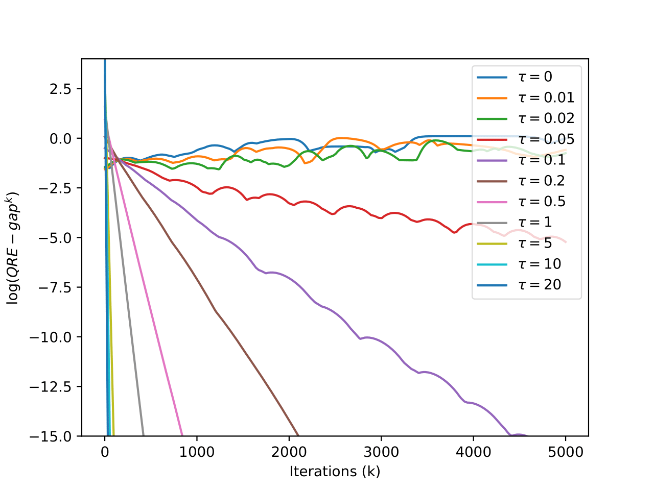
IV-A Synthetic Game Setting
We first consider a multi-agent system where the rewards are generated randomly and independently. We set the number of agents to , with each agent having a different discrete action space size, . At the start of the experiment, all agents are initialized with random policies. This setting is similar to that of [22]; however, the rewards assigned to the agents in [22] satisfy the potential game assumption, but they are set to be independent in our experiments. We use the same randomized reward and initial policy across a selection of regularization factors. The learning rate is set to , which is within the range given in Theorem III.3 that guarantees convergence.
The results are presented in Fig. 1 in log-scale. It can be seen that when there is no regularization, or the regularization factor is negligible, the system fails to converge. As increases, the system converges without strict monotonicity. When is large enough, the QRE-gap decreases monotonically and converges to zero at a linear rate, with the decay rate increasing as gets larger. The system dynamics in Fig. 1 perfectly verifies our finding on conditions of and the convergence rate in Theorem III.3.
Analytical results and experiments both indicate that the system converges faster when there is a larger weight on regularization, with the system actually failing to converge if the regularization term is too small. This observation aligns with our analytical results in Theorem III.3. In practice, a trade-off needs to be maintained, such that the system convergence is guaranteed, yet the QRE is still meaningful. Furthermore, we find that for the synthetic reward experiment above, a regularization factor of is enough for the system to converge with a linear rate. Interestingly, this requirement is significantly smaller than the requirement provided in Theorem III.3. This could be due to the random generation of rewards, whereas the theorem provides a bound in the worst-case scenario.
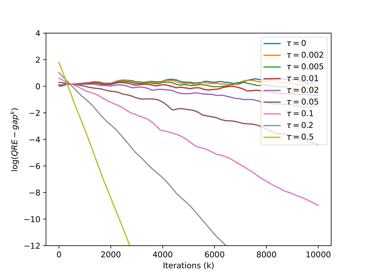
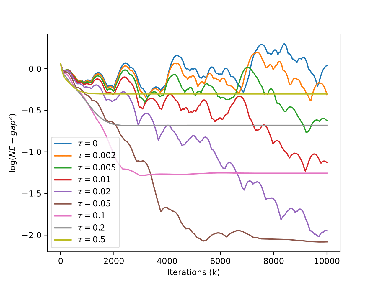
IV-B Network Zero-Sum Games
Next, we focus on the special game setting of zero-sum games in the network setting with polymatrix rewards [2]. This problem cannot be solved using the vanilla independent NPG update and requires additional design elements such as using extra-gradient methods [6]. However, most of the methods are restricted to the two-agent setting and cannot be adapted to the network setting.
We consider a 5-agent network with a ring graph. Each edge denotes a randomly generated zero-sum matrix game between the two neighbors. All agents are assumed to have the same action space .
We first present the QRE-gap in Fig. 2(a) (linear scale). It can be seen that the convergence properties in this setting mirror those of the synthetic game in Section IV-A. We also present the results on the NE-gap of the system shown in Fig. 2(b). As previously mentioned, NE-gap can be recovered by setting in QRE-gap. We note that NE-gap only depends on the current policy and is independent of the algorithm updates. The results largely mirror our first experiment, With a moderate regularization, the system is able to converge to stationarity with relatively small NE-gap. When the regularization term is too large, the system does converge but with a somewhat undesirable NE-gap.
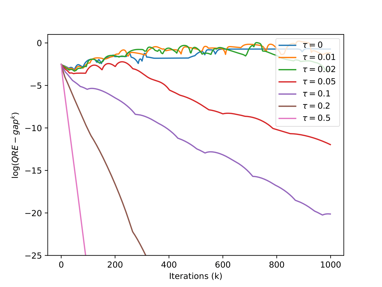
IV-C Markov Games
We now extend our experiments to the stochastic setting and use independent NPG to solve general Markov games. The Markov games setting can be seen as a generalization of the Markov decision process used in single-agent RL. Both the policy and reward depend on the current state of the system, which evolves according to a transition probability kernel , and the agent value function becomes a discounted cumulative reward.
We refer to [26] for the exact problem formulation and definition for natural gradients. We define the exact update for entropy-regularized NPG in Markov games as
where denotes the marginalized advantage function defined therein.
We consider a synthetic Markov game with agent number , each with action space , with the total number of states set to .
V CONCLUSIONS AND FUTURE WORKS
In this paper, we have studied the independent NPG algorithm with entropy regularization under the general multi-agent game setting. We have shown that the system converges to QRE under independent NPG updates, and that the rate of convergence is linear. However, such convergence only occurs with a sufficiently large regularization. On the other hand, a system with inadequate regularization may fail to converge. Experimental results were provided for both cases across various settings.
There are still many open problems that could be studied for policy gradient-based algorithms in games. A future direction of this work is to extend the analytical results to the stochastic (Markov) game setting. Our preliminary experiments have suggested that stochastic games could enjoy similar convergence to static games. This topic may contribute to multi-agent reinforcement learning, where the system is generally assumed to be Markov. Another potential direction is to consider the scenario where oracle information is unavailable, and the policy gradient needs to be estimated via sampling. Lastly, our analysis can be extended to policy gradient-based algorithms such as safe MARL, robust MARL, and multi-objective MARL, following recent literature in single-agent RL [28, 29].
VI ACKNOWLEDGMENTS
This material is based upon work partially supported by the US Army Contracting Command under W911NF-22-1-0151 and W911NF2120064, US National Science Foundation under CMMI-2038625, and US Office of Naval Research under N00014-21-1-2385.
References
- [1] Alekh Agarwal, Sham M Kakade, Jason D Lee, and Gaurav Mahajan. On the theory of policy gradient methods: Optimality, approximation, and distribution shift. The Journal of Machine Learning Research, 22(1):4431–4506, 2021.
- [2] James P Bailey and Georgios Piliouras. Multi-agent learning in network zero-sum games is a hamiltonian system. Momentum, 10:1, 2019.
- [3] Jupiter Bakakeu, Schirin Baer, Hans-Henning Klos, Joern Peschke, Matthias Brossog, and Joerg Franke. Multi-agent reinforcement learning for the energy optimization of cyber-physical production systems. Artificial Intelligence in Industry 4.0: A Collection of Innovative Research Case-studies that are Reworking the Way We Look at Industry 4.0 Thanks to Artificial Intelligence, pages 143–163, 2021.
- [4] Jalaj Bhandari and Daniel Russo. Global optimality guarantees for policy gradient methods. Operations Research, 2024.
- [5] Shicong Cen, Fan Chen, and Yuejie Chi. Independent natural policy gradient methods for potential games: Finite-time global convergence with entropy regularization. In 2022 IEEE 61st Conference on Decision and Control (CDC), pages 2833–2838. IEEE, 2022.
- [6] Shicong Cen, Chen Cheng, Yuxin Chen, Yuting Wei, and Yuejie Chi. Fast global convergence of natural policy gradient methods with entropy regularization. Operations Research, 70(4):2563–2578, 2022.
- [7] Shicong Cen, Yuejie Chi, Simon Shaolei Du, and Lin Xiao. Faster last-iterate convergence of policy optimization in zero-sum markov games. In The Eleventh International Conference on Learning Representations, 2022.
- [8] Shicong Cen, Yuting Wei, and Yuejie Chi. Fast policy extragradient methods for competitive games with entropy regularization. Advances in Neural Information Processing Systems, 34:27952–27964, 2021.
- [9] Constantinos Daskalakis, Dylan J Foster, and Noah Golowich. Independent policy gradient methods for competitive reinforcement learning. Advances in neural information processing systems, 33:5527–5540, 2020.
- [10] Tuomas Haarnoja, Aurick Zhou, Pieter Abbeel, and Sergey Levine. Soft actor-critic: Off-policy maximum entropy deep reinforcement learning with a stochastic actor. In International conference on machine learning, pages 1861–1870. PMLR, 2018.
- [11] Woojun Kim and Youngchul Sung. An adaptive entropy-regularization framework for multi-agent reinforcement learning. In International Conference on Machine Learning, pages 16829–16852. PMLR, 2023.
- [12] Guanghui Lan. Policy mirror descent for reinforcement learning: Linear convergence, new sampling complexity, and generalized problem classes. Mathematical programming, 198(1):1059–1106, 2023.
- [13] Yanli Liu, Kaiqing Zhang, Tamer Basar, and Wotao Yin. An improved analysis of (variance-reduced) policy gradient and natural policy gradient methods. Advances in Neural Information Processing Systems, 33:7624–7636, 2020.
- [14] Richard D McKelvey and Thomas R Palfrey. Quantal response equilibria for normal form games. Games and economic behavior, 10(1):6–38, 1995.
- [15] Jincheng Mei, Chenjun Xiao, Csaba Szepesvari, and Dale Schuurmans. On the global convergence rates of softmax policy gradient methods. In International Conference on Machine Learning, pages 6820–6829. PMLR, 2020.
- [16] Johannes Müller and Guido Montúfar. Geometry and convergence of natural policy gradient methods. Information Geometry, 7(Suppl 1):485–523, 2024.
- [17] John F Nash Jr. Equilibrium points in n-person games. Proceedings of the national academy of sciences, 36(1):48–49, 1950.
- [18] Guillaume Sartoretti, Yue Wu, William Paivine, TK Satish Kumar, Sven Koenig, and Howie Choset. Distributed reinforcement learning for multi-robot decentralized collective construction. In Distributed Autonomous Robotic Systems: The 14th International Symposium, pages 35–49. Springer, 2019.
- [19] Florian Schäfer and Anima Anandkumar. Competitive gradient descent. Advances in Neural Information Processing Systems, 32, 2019.
- [20] Shai Shalev-Shwartz, Shaked Shammah, and Amnon Shashua. Safe, multi-agent, reinforcement learning for autonomous driving. arXiv preprint arXiv:1610.03295, 2016.
- [21] Lloyd Shapley. Some topics in two-person games. Advances in game theory, 52:1–29, 1964.
- [22] Youbang Sun, Tao Liu, Ruida Zhou, PR Kumar, and Shahin Shahrampour. Provably fast convergence of independent natural policy gradient for markov potential games. Advances in Neural Information Processing Systems, 36, 2024.
- [23] Alexander Trott, Sunil Srinivasa, Douwe van der Wal, Sebastien Haneuse, and Stephan Zheng. Building a foundation for data-driven, interpretable, and robust policy design using the ai economist. Interpretable, and Robust Policy Design using the AI Economist (August 5, 2021), 2021.
- [24] Chen-Yu Wei, Chung-Wei Lee, Mengxiao Zhang, and Haipeng Luo. Last-iterate convergence of decentralized optimistic gradient descent/ascent in infinite-horizon competitive markov games. In Conference on learning theory, pages 4259–4299. PMLR, 2021.
- [25] Wenhao Zhan, Shicong Cen, Baihe Huang, Yuxin Chen, Jason D Lee, and Yuejie Chi. Policy mirror descent for regularized reinforcement learning: A generalized framework with linear convergence. SIAM Journal on Optimization, 33(2):1061–1091, 2023.
- [26] Runyu Zhang, Jincheng Mei, Bo Dai, Dale Schuurmans, and Na Li. On the global convergence rates of decentralized softmax gradient play in markov potential games. Advances in Neural Information Processing Systems, 35:1923–1935, 2022.
- [27] Runyu Zhang, Zhaolin Ren, and Na Li. Gradient play in stochastic games: stationary points, convergence, and sample complexity. IEEE Transactions on Automatic Control, 2024.
- [28] Ruida Zhou, Tao Liu, Min Cheng, Dileep Kalathil, PR Kumar, and Chao Tian. Natural actor-critic for robust reinforcement learning with function approximation. Advances in neural information processing systems, 2023.
- [29] Ruida Zhou, Tao Liu, Dileep Kalathil, PR Kumar, and Chao Tian. Anchor-changing regularized natural policy gradient for multi-objective reinforcement learning. Advances in Neural Information Processing Systems, 2022.
Appendix
VI-A Calculating the Policy Gradient
We provide the exact calculations of the derivative here. We note that
First by the chain rule of composition of derivatives,
where by the definition of , we can calculate as
We next compute the Jacobian matrix , for the -th element, we have
Therefore, we can write the derivative of
VI-B Proof of Lemma III.2
Proof:
We provide the proof for . For the case where , we can consider the first probability distributions as a joint distribution, and the lemma is proven by induction.
For , we denote the first set of policies as , and the second set as , respectively. We note that
The total variation distance can be bounded by the following inequality,
∎