Wobbling motion in triaxial nuclei

Abstract

The experimental evidence for the collective wobbling motion of triaxial nuclei is reviewed. The classification into transverse and longitudinal in the presence of quasiparticle excitations is discussed. The description by means of the quasiparticle+triaxial rotor model is discussed in detail. The structure of the states is analyzed using the spin-coherent-state and spin-squeezed-state representations of the reduced density matrices of the total and particle angular momenta, which distill the corresponding classical precessional motions. Various approximate solutions of the quasiparticle+triaxial rotor model are evaluated. The microscopic studies of wobbling in the small-amplitude random phase approximation are discussed. Selected studies of wobbling by means of the triaxial projected shell model are presented, which focus on how this microscopic approach removes certain deficiencies of the semi-microscopic quasiparticle+triaxial rotor model.

I Introduction

I review the work on the wobbling mode from my perspective. Section II discusses the triaxial rotor (TR) model. Based on its correspondence with the rotation of the classical TR, the TR eigenstates are classified as "wobbling" and "flip" states. The accuracy of this classification is justified. Section III is devoted to the particle+triaxial rotor (PTR) model. The classification of the PTR eigenstates as "transverse wobbling" (TW) and "longitudinal wobbling" (LW) based on the topology of the precession cones of the corresponding classical the angular momentum with respect to the principal axes is introduced. Subsection III.1 reviews the evidence for TW in strongly deformed nuclei, and discusses the details for a selected case. In the same way subsection III.2 reviews the evidence for TW in normal deformed nuclei. Three selected nuclei are discussed in detail, where the controversy about the TW interpretation is addressed. The instability of the TW mode and the transition to LW is discussed in subsection III.3. The evidence for LW in normal deformed nuclei is reviewed in subsection III.4. One selected case is presented in more detail. Subsection III.5 presents my perspective on the various approximate solutions of the PTR model. Section IV reviews the studies of the wobbling mode by means of the microscopic random phase approximation (RPA). Section V gives a short introduction to the microscopic description of wobbling in the frame work of the triaxial projected shell model (TPSM). It presents its application to two nuclei only because the TPSM is comprehensively reviewed in Chapter 11. Section VI addresses wobbling in nuclei with soft triaxiality.

II The triaxial rotor

Nuclei are composed of identical nucleons. This implies that the orientation of the nuclear density with respect to a symmetry axis cannot be specified, and collective rotation about this axis does not exist. The rational bands of deformed axial nuclei reflect the collective rotation about the axis perpendicular to the symmetry axis. The axial rotor Hamiltonian is simply $(\hat{R}^{2}-\hat{R}_{3}^{2})/2{\cal J}$ with 3 being the symmetry axis and ${\cal J}$ the moment of inertia (MoI). For reflection-symmetric nuclei the rotational band built on the ground state is the sequence $I(I+1)/2{\cal J}$, $I$= 0, 2, 4, …. The odd $I$ do not appear because a rotation ${\cal R}_{\bot}(\pi)$ about an axis perpendicular to the symmetry axis leaves the intrinsic state of the rotor invariant. In their textbook BMII , Bohr and Mottelson discussed in detail the rotational features of the axial rotor when the intrinsic state contains excited quasiparticles.

For triaxial shape, specified by the deformation parameters $\beta$ and $\gamma$, (see BMII ) collective rotation about the third axis becomes possible. The new degree of freedom leads to a new class of collective excitations - the "wobbling" mode, which is described by the triaxial rotor Hamiltonian

$$H_{\textrm{TR}}=\sum_{i=1,2,3}A_{i}\hat{J}_{i}^{2},~{}~{}~{}A_{i}=\frac{1}{2{\mathcal{J}_{i}}},$$ (1)

where $i$ refers to the three principal axes of the triaxial density distribution.

The model parameters are the three MoI’s $\mathcal{J}_{i}$. Their choice is restricted by the fundamental condition that collective rotation about a symmetry axis is not allowed. More specifically, the more the density of a principal axis deviates from rotational symmetry the larger is its MoI, which requires the order $\mathcal{J}_{m}>\mathcal{J}_{s}>\mathcal{J}_{l}$. In the following, we associate the axes $i$= 1, 2, 3, with the short, medium, and long principal axes of the density distribution, respectively, using the short-hand notation $s-$, $m-$ and $l-$ axes.

The eigenstates are determined by the asymmetry parameter of the MoI’s

$$\kappa=\frac{2A_{1}-A_{2}-A_{3}}{A_{2}-A_{3}},~{}~{}A_{2}\leq A_{1}\leq A_{3}.$$ (2)

The inertia ellipsoid changes from a prolate spheroid for $\kappa=-1,~{}A_{1}=A_{3}$ to an oblate spheroid for $\kappa=1,~{}A_{1}=A_{2}$ with maximal triaxiality at $\kappa=0$.

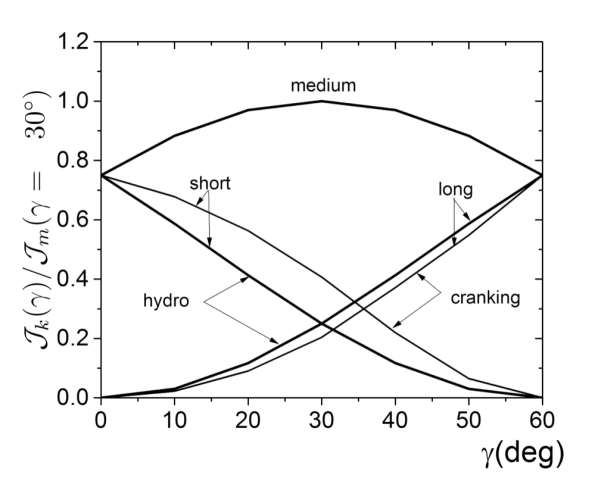
Figure 1: Thick curves: Irotational flow MoI’s as functions of the triaxiality parameter $\gamma$ (Copenhagen convention). Thin curves: Microscopic cranking calculations for $Z=68$, $N=96$, $\Delta_{p}=1.1$ MeV, $\Delta_{n}=1.0$ MeV, $\varepsilon=0.25$. Reproduced with permission from Ref.  Frauendorf2018PRC (where the Lund convention with the opposite sign of $\gamma$ was used).

.

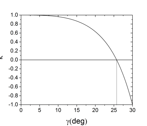
Figure 2: The asymmetry parameter $\kappa(\gamma)$ Eq. (2) for irrotational flow MoI’s.

The condition is obeyed by the assumption that the ratios between MoI’s agree with the ones of irrotational flow of an ideal liquid BMII Eq. (6B-17),

$$\mathcal{J}_{i}(\beta,\gamma)=\mathcal{J}_{0}(\beta)\sin^{2}\left(\gamma-\frac{2\pi i}{3}\right),$$ (3)

where $\mathcal{J}(\beta)$ sets the scale. Fig. 1 shows the irrotational-flow MoI’s and Fig. 2 the pertaining asymmetry parameter as functions of $\gamma$. Below $15^{\circ}$, where ${\cal{J}}_{3}$ is small, the inertia ellipsoid does not change much. For $\gamma=25.76^{\circ}$ it is maximal triaxial. Above, it rapidly develops to a prolate spheroid with ${\cal{J}}_{2}>>{\cal{J}}_{1}\approx{\cal{J}}_{3}$.

The analysis of of the rotational energies and E2 matrix element from COULEX experiments  Allmond2017PLB demonstrated that the dependence of MoI’s on the triaxiality parameter $\gamma$ is well accounted for by Eq. (3). Microscopic calculations by means of the cranking model Frauendorf2018PRC demonstrated that the MoI’s approach the ratios (3) for strong pairing correlations. Fig. 1 includes the MoI’s for realistic pairing. For weak pairing substantial deviations appear. However the deviations do not indicate an approach to the ratios of rigid body flow, because these contradict the no-rotation-about-a-symmetry-axis restriction of the nuclear many body system. The moment of the medium axis is always the largest because the density distribution maximally deviates from axial symmetry.

Not all solutions of the triaxial rotor (TR) Hamiltonian are accepted for nuclei. Restricting the discussion to the case that the intrinsic triaxial ground state is invariant with respect to the three rotations ${\cal R}_{i}(\pi)$ only the TR solutions that are symmetric with respect to the three rotations are rotational excitations of the intrinsic ground state (completely symmetric representations of the D₂ point group) are allowed..

The TR Hamiltonian is diagonalized in the basis of the axial rotor states $|IMK\rangle$, where $M$ is the angular momentum projection on the laboratory $z$-axis and $K$ the projection the 3-axis axes of the rotor. The TR eigenstates

$$|IM\nu\rangle=\sum_{K=-I}^{I}C_{IK}^{(\nu)}|IMK\rangle$$ (4)

are given by the amplitudes $C_{IK}^{(\nu)}$, which depend only on $K$. the angular momentum projection on one of the body-fixed principal axes. The symmetry restricts $K$ to be even and requires $C_{I-K}^{(\nu)}=(-1)^{I}C_{IK}^{(\nu)}$.

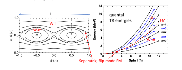
Figure 3: Left panel: Classical orbits of the triaxial rotor states that are connected by the vertical line at $I=8$ the right panel. The energies are equal to their quantal energies in the right panel, labelled in ascending order. Right panel: Energies of the triaxial rotor as functions of the angular momentum $R$. The states are labelled by the wobbling quantum number $n$. The dashed line represents the energy of the separatrix $I(I+1)/(2\mathcal{J}_{s})$. Reproduced with permission from Ref. Chen_Frauendorf2022EPJA and Frauendorf2014PRC and augmented.

The right panel of Fig. 3 shows the TR energies with the MoI’s $\mathcal{J}_{m}=30~{}\hbar^{2}$/MeV, $\mathcal{J}_{s}=10~{}\hbar^{2}$/MeV, $\mathcal{J}_{l}=5~{}\hbar^{2}$/MeV. Their ratios correspond to $\kappa=0.24$, which is close to 0 of maximal asymmetry oft the inertia ellipsoid. It is instructive to classify the states using quasiclassic correspondence. The left hand panel shows the classical orbits of the angular momentum vector $\mathbf{R}$ with respect to the principal axes of the triaxial shape, where

$$R_{1}=R\sin\theta\cos\phi,~{}R_{2}=R\sin\theta\sin\phi,~{}R_{3}=R\cos\theta.$$ (5)

The orbits are determined by the conservation of the angular momentum $R^{2}=I(I+1)$ and the energy $E_{TR}(I)$, Eq. (1), which is set equal to the quantal energies in right panel. The panel shows the orbits for the states $I_{\nu}=8_{\nu}$ which are connected by the vertical line at $I=8$ in the right panel. There are two types of orbits, which are separated by the separatrix shown as the dashed orbit in the left panel. For the states inside the separatrix the angular momentum revolves around the $m$-axis with the maximal MoI, and for the ones outside it revolves around the $l$-axis with the minimal MoI. The orbits are numbered by their energy in ascending order. For the lowest states the motion is harmonic as seen by the elliptic shape of the orbit.

Using semiclassical correspondence the states are classified by their topology. On page 190 of their textbook Nuclear Structure II BMII Bohr and Mottelson introduced the name "wobbling" as "…the precessional motion of the axes with respect to the direction of I; for small amplitudes this motion has the character of a harmonic vibration… ". This clearly describes the states that correspond to the orbits inside the separatrix. Hence it is appropriate to call these states wobbling excitations. Accordingly, the states labelled by $n=$ 0, 1, 2, ….are called zero, single, double, … wobbling excitation, respectively. In Ref. Lawrie2020 (see Chapter 6) the authors suggested restricting the name "wobbling" to the elliptic (harmonic) precession cones and call the other tilted precession (TiP) cones (see the detailed discussion below). In my view this is an unnecessary complication. It does not comply with Bohr and Mottelson, who associate wobbling with a general precession and then add harmonic vibration as a special case. I recommend using the simple topological classification with respect to the separatrix.

It is instructive indicating the axis about which the angular momentum vector precesses. In the TR model one has the m-axis wobbling states which correspond to the orbits inside the separatrix and the l-axis wobbling states which correspond to the orbits outside it.

Classically, the separatrix represent the unstable rotation about the s-axis with the intermediate MoI. The orbits in its vicinity represent a number of revolutions about the unstable axis and then a rapid change to rotation about the opposite orientation of the unstable axis for another number of revolutions and back to the original orientation, and so on. This behavior of the triaxial top is also known as the Dzhanibekov effect after the Russian cosmonaut who observed it when he unscrewed a wing nut, which flipped off his hand and floated around. Instructive videos can be found in Wikipedia. In Ref. Chen_Frauendorf2022EPJA , Chen and Frauendorf suggested the name "flip mode" (FM) for the states corresponding to orbits close to the separatrix. The right panel of Fig. 3, demonstrates how new FM states are born at the energy of the separatrix while the lowest wobbling states become more and more harmonic when the angular moment increases. The anharmonicity of the mode increases with the wobbling number $n$. There is no sharp borderline between the wobbling and flip regimes.

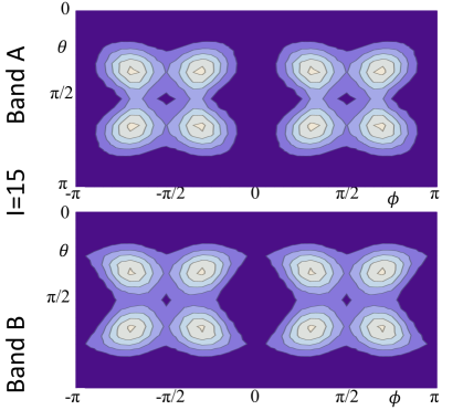
Figure 4: Probability distribution of the angular momentum orientation $P(\theta\phi)_{I\nu}$ generated from the reduced density matrix of the particle-hole plus TR calculation for ¹³⁴Pr in Ref. Stefan-Jie. The SCS map shows that the distributions of the chiral partner bands are almost the same at $I=15$ where the two bands are nearly degenerate. Reproduced with permission from Ref. Frauendorf2015Conf .

The Spin Coherent State (SCS) representation distills the semiclassical features from the TR states. The probability of the angular momentum orientation is given by

$$P(\theta\phi)_{I\nu} =\frac{2I+1}{4\pi}\sin\theta$$

$$\times\sum\limits_{K,K^{\prime}=-I}^{I}D^{I*}_{IK}(0,\theta,\phi)\rho^{(\nu)}_{KK^{\prime}}D^{I}_{K^{\prime}I}(0,\theta,\phi).$$ (6)

In the case of the TR the density matrix is

$$\rho^{(\nu)}_{KK^{\prime}}=C^{(\nu)}_{IK}C^{(\nu)*}_{IK^{\prime}}$$ (7)

with $\nu=n$ being the wobbling number. Plots of $P(\theta\phi)_{I\nu}$ (SCS maps) have first been produced for the two-particle triaxial rotor model  Frauendorf2015Conf (see Fig 4) in order to visualize the appearance of the chiral geometry of the quantal results. In these cases $\rho^{(\nu)}_{KK^{\prime}}$ is the reduced density matrix. Subsequently Chen et al. F.Q.Chen2017PRC published the visualization technique under the name “azimuthal plots" for the projected shell model. Later on it has been used quite a bit to illustrate the chiral and wobbling geometry.

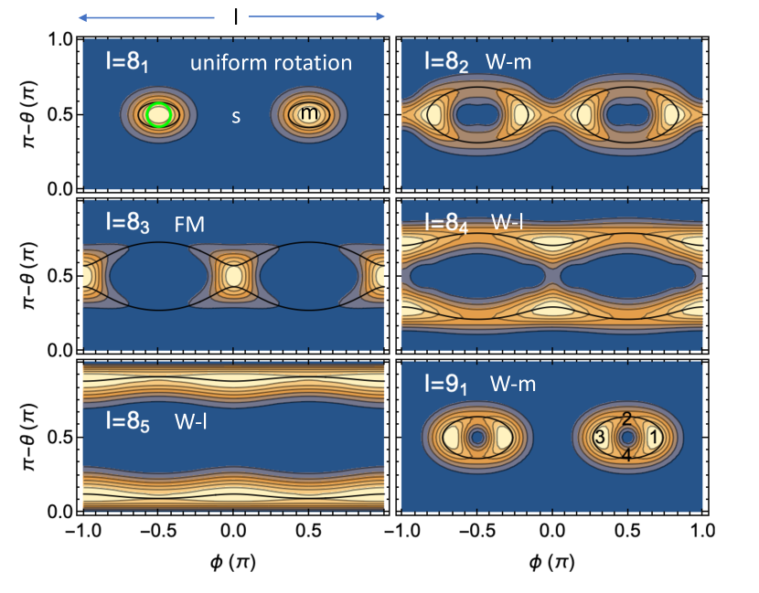
Figure 5: SCS probability densities of the angular momentum orientation $P(\theta\phi)_{I\nu}$ of the triaxial rotor states $I_{\nu}=8_{1}$, … $8_{5}$ and $9_{1}$ shown in Fig. 3. The states are labelled by $I_{\nu}$ in direction of ascending energy. The color sequence with increasing probability is dark blue $-$ zero, light blue, dark brown, light brown, white. The densities are normalized. The classical orbits are shown as black full curves. The energies are equal to their quantal energies in Fig. 3. The numbers indicate the turning points. The green circle indicates the finite resolution of the plot caused by the non-orthogonaliy of the SCS basis. Reproduced with permission from Ref. Chen_Frauendorf2022EPJA .

The SCS map in Fig. 5 shows that the distributions are fuzzy rims tracing the classical orbits, which are included as black curves. As discussed in detail in Ref. Chen_Frauendorf2022EPJA , the quantal values of $P(\theta\phi)_{I\nu}d\sin\theta d\phi$ correspond to the ratio $dt/T$ of the time $dt$ the classical orbit spends within the area $d\sin\theta d\phi$ and $T$ the time for one revolution.

Inspecting the figure, it is instructive to remember the physical pendulum, for which the elongation angle $\varphi$ and the momentum $p=\mathcal{J}d\varphi/dt$ are canonical variables. In analogy, the angle $\phi$ and $R_{3}=R\cos\theta$ are the conjugate position and momentum of the classical TR. For small energy the motion is harmonic (mathematical pendulum), and the phase space curve is an ellipse. With increasing energy the curve deforms. Along with this, the time near the two turning points increases and the time near $\phi=\pi/2$ or $\varphi=0$ deceases. At the critical energy of the separatrix the pendulum takes the unstable position $\varphi=\pm\pi$ and the TR the position $\phi=0$ corresponding to the unstable rotation about the s-axis. For energies slightly below the pendulum stays a long time at the turning points to swing rapidly through $\varphi=0$. For energies slightly above the pendulum very slowly passes over $\varphi=\pi$ and keeps going, i. e. it rotates about its axis. The relative passage time through $\varphi=\pi$ decreases with a further increase of the energy. In analogy, for energies above the critical value the TR angular momentum precesses around the l-axis instead about the m-axis as for the energies below. For energies near the critical value the TR angular momentum vector stays very long near the s-axis and moves rapidly through $\phi=\pi/2$, like the rapid passage of $\varphi=0$ of the pendulum.

The state $8_{3}$ has an energy somewhat above the critical value. Its angular momentum stays long near the s-axis $\phi=0$, rapidly moves (flips) to the negative s-axis $\phi=\pm\pi$, stays long, flips back to the positive s-axis $\phi=0$, and so on. Accordingly it is called the "flip mode" and labelled by FM in Fig. 3, where the lower states are labelled as W-m and the higher as W-l according to their precession axes.

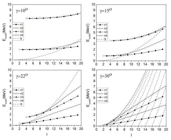
Figure 6: Experimental wobbling energies Eq. (8) for $\gamma=10^{\circ},~{}15^{\circ},~{}22^{\circ},~{}30^{\circ}$ assuming irrotational-flow MoI’s Eq.(3). The respective inertia asymmetry parameters are $\kappa=$ 0.96, 0.87, 0.47, -1. The energies are normalized to $E(2^{+}_{1})$. The dashed curves show the separatrix, except for $\gamma=30^{\circ}$, where they connect the sequences with the same projection $K$ on the m-axis.

"Experimental" wobbling energies of the TR spectrum are defined as the excitation energies above the yrast states,

$$E_{w}(I)=E(I)-\left(E(I-1)_{yrast}+E(I+1)_{yrast}\right)/2$$ (8)

Fig. 6 shows $E_{w}(I)$ of the TR with irrotational-flow MoI’s for different $\gamma$. For the lowest states and sufficiently high angular momentum, located far enough below the separatrix, the harmonic approximation BMII , p. 190 ff, Frauendorf2014PRC becomes valid. The TR energies are given by

$$E_{n}(I)=A_{3}I(I+1)+\left(n+\frac{1}{2}\right)\hbar\omega_{w},~{}~{}A_{i}=1/2\mathcal{J}_{i}$$ (9)

where $n$ is the number of wobbling quanta and the wobbling frequency $\hbar\omega_{w}$ is equal to

$$\hbar\omega_{w}=2I\,[(A_{1}-A_{2})(A_{3}-A_{2})]^{1/2}.$$ (10)

Reduced transition probabilities are given in Refs. BMII and Frauendorf2014PRC (where the different axes assignment $A_{1}\geq A_{2}\geq A_{3}$ was used). An example is the case $\gamma=22^{\circ}$ with $\kappa$=0.47 in Fig. 6, where for $I>15$ the distance between lowest wobbling excitations $n$=1, 2, 3 is about the same.

For $\gamma=30^{\circ}$ the irrotational-flow MoI’s have the ratios $\mathcal{J}_{m}:\mathcal{J}_{s}:\mathcal{J}_{l}=4:1:1$. The TR is a symmetric top (Meyer-ter-Ven limit MtV1975 ) with the energy expression

$$E_{n}(I)=I(I+1)A_{s}+K^{2}(A_{m}-A_{s}),$$ (11)

where $K=I-n$ is the angular moment projection on the m-axis, which takes even values between $I$ and $-I$. The expressions for the transition probabilities can be obtained from Ref. BMII by relabelling the axes.

The states group into sequences of fixed $K$, which are displayed by the dashed curves in Fig. 6. The full lines display the lowest bands to be seen experimentally. As usual, these states are connected by strong E2 transitions. Their corresponding classical motion is a precession of the angular momentum around the m-axis, where the orbit in the s-l-plane is a circle with the radius $n=I-K$, which is a special case of wobbling. When $\gamma$ increases toward $30^{\circ}$ the elliptical orbits develop into circles and the separatrix approaches the $K=0$ sequence.

Lawrie et al. Lawrie2020 (see Chapter 6) introduced a different terminology for the classical orbits. They restrict the name wobbling to the elliptical orbits which can be approximated as harmonic oscillations. All other orbits are called Tilted Precessions (TiP). The qualitative properties of the TiP orbits are described as the ones of the $\gamma=30^{\circ}$symmetric top, and the authors use the angular momentum projection on the m-axis $K$ to label the TiP bands. The TR Hamiltonian (1) is more general, it encompasses different MoI’s for all three axes for which the TiP approximation does not hold. On the other hand, the harmonic approximation for wobbling by Eqs. (9, 10) and the pertaining expressions for the transition probabilities hold up to small terms of the order of $1/I$ for the lowest bands of the $\gamma=30^{\circ}$ TR (see Fig.1 of Ref. Lawrie2020 ), which makes the TiP terminology inconsistent. Moreover "tilted precession", as meant by the authors, is a tautology, because in a precession cone the angular momentum vector is tilted with respect to the axis it revolves by definition.

In my view, it is better keeping the terminology simple and call all the states that correspond to the orbits which revolve around the m-axis wobbling states, irrespective if the precession is harmonic or not. The name is quite appropriate, because the change of the rotational axis of the earth, which is quite irregular, and the tumbling of the rotational axis of a baseball are both called wobbling motion. It is also consistent with the way Bohr and Mottelson introduced the name into nuclear physics (see above). The first phrase indicates a general precessional mode, the second phrase indicates the special case of small amplitude motion, which is worked out in the book.

In Fig. 6 $\gamma=10^{\circ}$ illustrates the other case of small asymmetry of the inertia tensor $\kappa=0.96$, with the MoI’s ratios $\mathcal{J}_{m}:\mathcal{J}_{s}:\mathcal{J}_{l}=29:19:1$. The separatrix is close to the yrast line, such that the $n=1$ wobbling state appears only for $I\geq 17$. For smaller $I$ the lowest excited states form a doublet, which correspond to a narrow precession cone around the l- axis. The SCS maps show maxima at $\theta=\pi/2,~{}\phi=0,~{}\pm\pi$ for even $I$ and $\theta=\pi/2,~{}\phi=\pm\pi/2$, which represent the near-axial density distribution $\propto|D^{I}_{I,2}(0,\theta,\phi)+(-1)^{I}D^{I}_{I,-2}(0,\theta,\phi)|^{2}$. The doublet sequence has the characteristics of the $\gamma$ band of axial nuclei. As already pointed in Ref. BMII , the properties of the $\gamma$ band are well accounted for by a slightly asymmetric TR. Examples are the experimental information on the E2 matrix elements in ¹⁶⁸Er (TR $\gamma=7^{\circ}$) Frauendorf2018 and the work in Ref. Allmond2017PLB . The $\gamma$ vibration represents a wave that travels around the l- axis of the axial nucleus, which is equivalent with the $K=2$ excitation of a TR with weak triaxiality.

Figure 7: Experimental wobbling energies Eq. (8) for ¹¹²Ru (full symbols) compared with the TR calculation (open symbols) using irrotational-flow MoI’s for $\gamma=19^{\circ}$ and ${\cal J}_{0}=30(1+0.2I)\hbar^{2}/\mathrm{MeV}$.

Fig. 7 compares the $n=1,~{}2$ wobbling bands in ¹¹²Ru ensdf with the a TR calculation assuming irrotational flow, Eq. (3) with $\gamma=19^{\circ}$, and the variational moment of inertia (VMI) ${\cal J}_{0}=30(1+0.2~{}I)\hbar^{2}/\mathrm{MeV}$. With increasing $I$ the structure changes from the a flip mode to anharmonic wobbling. The use of the VMI is decisive for the good agreement with the experimental wobbling energies. However, it renders too low energies for the ground band. It is not possible to adjust $\gamma$ and ${\cal J}_{0}$ such that good agreement for both the wobbling and yrast energies is achieved.

The case of ¹¹²Ru together with ⁷⁶Ge Toh13 and ¹⁹²Osensdf are the scarce examples of wobbling excitations on the ground state band. There is a larger number of even-even nuclei for which the even-I sequence of the quasi $\gamma$ band is lower than the odd-I one, while for wobbling the order is opposite. This "staggering of the $\gamma$ band" indicates whether respectively, the deviation from axial shape is dynamic or static or, as commonly said, the nuclei are $\gamma$ soft or rigid (see e. g. Refs. Frauendorf15 ; Ruoof2024 ). In Refs. Ruoof2024 ; SJ21 ; Na23 the authors demonstrated that the microscopic triaxial projected shell model (TPSM) JS99 very well describes the experimental energies and E2 matrix elements of both $\gamma$ rigid and soft nuclei, provided the coupling to the quasiparticle excitations is taken into account (see Section VI). This microscopic approach removes the problem with the yrast energies of the phenomenological TR description of ¹¹²Ru (See Figs. 5 and 7 and Tab. 3 of Ref. Ruoof2024 ) It would be interesting to investigate the angular momentum geometry of $\gamma$ soft nuclei.

III Particles coupled to the triaxial rotor

The experimental evidence for wobbling is clearer when one or more high-j particles are coupled to the TR, because their interaction stabilizes the triaxial shape. The high-j particles act like gyroscopes, which change the wobbling motion. The Particle plus Triaxial Rotor (PTR) model MtV1975 describes the coupled system and has become a standard tool for interpretation. The corresponding Hamiltonian is MtV1975 ; BMII

$$H_{\textrm{PTR}}=\sum\limits_{i=1,2,3}\frac{(\hat{J}_{i}-\hat{j}_{i})^{2}}{2{\cal J}_{i}}+h_{p}(\gamma),$$ (12)

where $\hat{J}_{i}=\hat{R}_{i}+\hat{j}_{i}$ is the total angular momentum, $\hat{j}_{i}$ the angular momentum of the particle, $\hat{R}_{i}$ the one of the triaxial rotor, and $h_{p}(\gamma)$ describes the coupling of the particle with the triaxial potential. If necessary, the pair correlations are taken into account by applying the BCS approximation to $h_{p}$. In this case the model is called the quasiparticle triaxial rotor (QTR) model. In the following I will refer to both PTR and QTR even when the pair correlations are unimportant. The coupling of the high-j particles $f_{7/2},~{}h_{11/2}~{}i_{13/2},~{}j_{15/2}$ is often described by the simplified Hamiltonian Hamamoto1986PLB which assumes that their angular momentum is conserved

$$h_{p}(\gamma)=\frac{\kappa}{j(j+1)}\left[\left(3j_{3}^{2}-j(j+1)\right)\cos\gamma+\sqrt{3}\left(j_{1}^{2}-j_{2}^{2}\right)\sin\gamma\right].$$ (13)

The coupling strength $\kappa$ is determined by adjusting the single particle energies generated by $h_{p}(\gamma)$ to the ones of a realistic triaxial nuclear potential of the same triaxiality parameter $\gamma$. As the shape of the neutron and proton densities are very similar the same $\gamma$ value determines the intrinsic charge quadrupole moments and the $E2$ transition probabilities as well. The inclusion of pairing and the generalization to quasiparticles is straightforward Hamamoto1986PLB . The MoI’s are input parameters which are confined by the conditions of the TR discussed in section II. In some studies the irrotational ratios (3) for the same value of $\gamma$ as for the particle potential are used, and only ${\cal J}_{0}$ is adjusted to the rotational energies. In most studies some deviation of the inertia asymmetry $\kappa$ (not to be confused with $\kappa$ in Eq. (13)) from the irrotational value is accepted as long as the general conditions ${\cal J}_{m}>{\cal J}_{s}>{\cal J}_{l}$ are met. (See chapter 10 for examples.)

The PTR eigenstates are represented in the basis $|IIK\rangle|jk\rangle$, where $|IIK\rangle$ are the rotor states for half-integer $I$ and $|jk\rangle$ the high-$j$ particle states,

$$|II\nu\rangle=\sum_{K,k}C_{IKk}^{(\nu)}|IIK\rangle|jk\rangle.$$ (14)

The coefficients $C_{IKk}^{(\nu)}$ are restricted by requirement that rotor-core states must be symmetric representations of the D₂ point group, which implies

$$C_{I-K-k}^{(\nu)}=(-1)^{I-j}C_{IKk}^{(\nu)},~{}~{}K-k~{}~{}\mathrm{even}.$$ (15)

Expression for the transition probabilities are given for example in Ref. Chen_Frauendorf2024 . The reduced density matrices

$$\rho_{kk^{\prime}}^{(\nu)}=\sum_{K}C_{IKk}^{(\nu)}C_{IKk^{\prime}}^{(\nu)*}$$ (16)

and

$$\rho_{KK^{\prime}}^{(\nu)}=\sum_{k}C_{IKk}^{(\nu)}C_{IK^{\prime}k}^{(\nu)*}$$ (17)

are inserted into Eq. (II) to generate SCS maps, which illustrate the corresponding motion of the particle $\mathbf{j}$ and total angular momentum $\mathbf{J}$, respectively.

III.1 Transverse wobbling in triaxial strongly deformed nuclei

Clear evidence for wobbling in triaxial strongly deformed (TSD) nuclei was established by the Copenhagen group. They found in ^161-167Lu 161Lu ; 163Lu1 ; 163Lu2 ; 165Lu ; 167Lu and ¹⁶⁷Ta 167Ta very regular bands in the spin range $I\approx 15-40$, which are based on the $i_{13/2}$ proton orbital and a deformation of $\beta\approx 0.4$. The bands TSD2 $\rightarrow$ TSD1 and TSD3 $\rightarrow$ TSD2 are interconnected by strong $I\rightarrow I-1$ collective $E2$ transitions, which are the hallmark of the wobbling motion of the charge density of the whole nucleus. The bands TSD1, TSD2, TSD3 were assigned to carry $n=$0, 1,2 wobbling quanta, respectively. Hamamoto and Hagemann 163Lu1 ; hamamoto1 ; hamamoto2 carried out PTR calculations. They assumed $\gamma=20^{\circ}$, irrotational flow MoI’s and adjusted $\kappa{\cal J}_{0}$ to account for the average wobbling energy. However, the authors exchanged the MoI such that ${\cal J}_{s}$ is largest and ${\cal J}_{m}$ is second in contrast to the order implied by the principles of spontaneous symmetry breaking.

The PTR system has the particle degrees of freedom in addition to the orientation of the total angular momentum. The authors illustrated the pertaining types of excitations in Fig. 8. The $i_{13/2}$ proton has the lowest energy when its angular momentum $\mathbf{j}$ aligns with the s-axis, because this orientation generates the best overlap with the triaxial potential (See the discussion of particle alignment in Ref. Frauendorf2018 ). In the yrast band (TSD1) the TR angular momentum $\mathbf{R}$ aligns with the s-axis as well. In panel (a) the proton $\mathbf{j}$ is tilted from the s-axis about which it precesses while $\mathbf{R}$ stays aligned. This is the excitation type that the cranking model describes as a signature partner band (The signature is defined as $\alpha=I+2n$.) In panel (b) the proton $\mathbf{j}$ stays aligned while the $\mathbf{R}$ is tilted from the s-axis about which it precesses. This the first wobbling excitation. It generates strong E2 radiation, which is not the case for the signature partner band. The difference can be used to identify the bands as wobbling or cranking excitations.

The PTR $\frac{B(E2,I\rightarrow I-1)_{out}}{B(E2,I\rightarrow I-2)_{in}}$ ratios in Fig. 9 agree well with the experimental ones. The ratio of 0.2 indicates a strong collective enhancement of the inter band E2 transitions, which the hallmark of the wobbling mode. However the PTR energy difference between the $n_{w}=0$ yrast band the $n_{w}=1$ wobbling bands increases with $I$, which is in contrast to the decrease of the distance between the bands TSD2 and TSD1. The authors noticed that the natural order ${\cal J}_{s}<{\cal J}_{m}$ leads to a decrease of the wobbling energy, but dismissed it, because it was too rapid.

The studies of ^161,165,167Lu 161Lu ; 165Lu ; 167Lu rendered similar wobbling behavior as ¹⁶³Lu. The accordance of $\frac{B(E2,I~{}n=2\rightarrow I-1,~{}n=1)_{out}}{B(E2,I\rightarrow I-2)_{in}}$ ratios with the PTR calculations is the same as for ¹⁶³Lu.

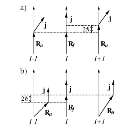
Figure 8: Schematic coupling scheme of the particle and core angular momenta in the favored ($I$) and unfavored ($I\pm 1$) states for (a) the cranking regime and (b) the wobbling mode ($n_{w}=1$). Reproduced with permission from Ref. 163Lu1 .

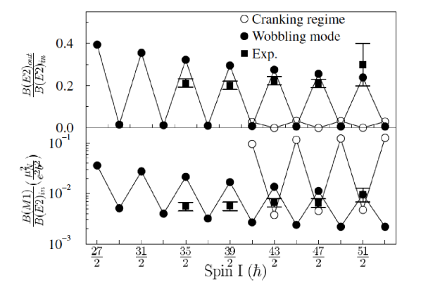
Figure 9: Ratios $\frac{B(E2,I\rightarrow I-1)_{out}}{B(E2,I\rightarrow I-2)_{in}}$ and $\frac{B(M1,I\rightarrow I-1)_{out}}{B(E2,I\rightarrow I-2)_{in}}$ between the bands TSD2 and TSD1 compared with the PTR calculation in Refs. 163Lu1 ; hamamoto1 ; hamamoto2 . Reproduced with permission from Ref. 163Lu1 .

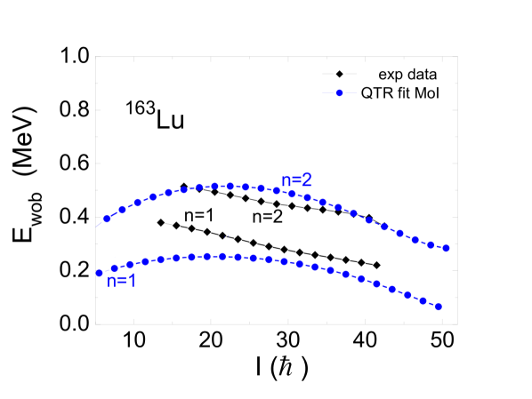
Figure 10: Experimental wobbling energies Eq. (8) of the bands TSD2 and TSD3 in ${163}$Lu compared with the PTR (labelled by QTR) calculations in Ref. Frauendorf2014PRC using the parameters $\varepsilon=0.4,~{}\gamma=20^{\circ},~{}{\cal J}_{m,s,l}=(64,56,13)\hbar^{2}$/MeV, respectively. Reproduced with permission from Ref. Frauendorf2014PRC .

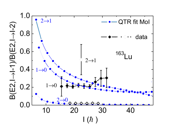
Figure 11: Ratios $\frac{B(E2,I\rightarrow I-1)_{out}}{B(E2,I\rightarrow I-2)_{in}}$ and $\frac{B(M1,I\rightarrow I-1)_{out}}{B(E2,I\rightarrow I-2)_{in}}$ between the bands TSD2 and TSD1 compared with the QTR calculations in Ref. Frauendorf2014PRC . Reproduced with permission from Ref. Frauendorf2014PRC .

The exchange of the two MoI’s appears to be a serious problem because it violates a basic principle of spontaneous symmetry breaking. Analyzing their PTR calculations, Frauendorf and Meng discovered that the rotational motion of odd-odd nuclei may attain a chiral character Frauendorf-Meng97 (c.f. Figs. 2b and 5 of Ref. Frauendorf-Meng97 and Chapter 3 of this book). The chiral geometry emerges as the combination of the angular momenta of a proton particle, a neutron hole and the TR core aligned with the s- axis, the l-axis and the m-axis, respectively. That is, chirality appears because the m-axis has the larges MoI. Fig. 2a of Ref. Frauendorf-Meng97 demonstrates that the rotational spectrum is analogous when both the proton and the neutron are holes with their angular momentum aligned with the l-axis. The distance between the lowest even and odd $I$ bands decreases with $I$. The same kind of decrease is expected in the spectrum of the TR combined with one proton with its angular momentum aligned with the s-axis, which is observed in the Lu isotopes. To arrive at an interpretation which is consistent with the extended work on chirality by then, Frauendorf and Dönau Frauendorf2014PRC reanalyzed the TSD bands of the Lu isotopes by means of the QTR, requiring that the m-axis has the largest MoI.

The authors carried out QTR calculations with the same deformation parameters $\varepsilon=0.4$ and $\gamma=20^{\circ}$ as in Refs. 163Lu1 ; hamamoto1 ; hamamoto2 . (The actual calculations were carried out in the framework of the core-quasiparticle-coupling model (QCM), which for the TR core is just the PTR or QTR reformulated in the laboratory frame. See Section VI and Ref. Frauendorf2014PRC .) Three sets of MoI’s were investigated which obey the requirement that ${\cal J}_{m}$ is the largest. Figs. 10 and 11 compare the energies and $\frac{B(E2,I\rightarrow I-1)_{out}}{B(E2,I\rightarrow I-2)_{in}}$ ratios with the ones from TSD2 and TSD3. The ratios between the TR MoI’s were adjusted to obtain the best agreement of the wobbling energies with experimental ones. The corresponding inertia asymmetry of $\kappa=0.93$ is close to $\kappa=0.91$ for the microscopic MoI’s obtained by the cranking model, which gave results very similar to the ones in Figs. 10 and 11. The irrotational flow MoI’s for $\gamma=20^{\circ}$ correspond to $\kappa=0.64$. The enhanced asymmetry of the inertia ellipsoid causes a too steep decrease of the wobbling energy with $I$. Thus, the features of the TSD wobbling bands are well accounted for by the QTR applying it in consistency with the studies of chirality. The only caveat is an overestimate of the $\frac{B(M1,I\rightarrow I-1)_{out}}{B(E2,I\rightarrow I-2)_{in}}$ ratios.

In order elucidate the physics behind the decreasing wobbling energy Dönau and Frauendorf Frauendorf2014PRC drastically simplified the PTR by assuming that the proton $\mathbf{j}$ is rigidly aligned with the s-axis, which they called the frozen alignment (FA) approximation.

$$H_{FA}=A_{1}(\hat{J}_{3}-j)^{2}+A_{2}\hat{J}_{1}^{2}+A_{3}\hat{J}_{2}^{2},$$ (18)

where $j$ is a number.

Applying the small-amplitude approximation

$$\hat{J}_{3}=(\hat{J}^{2}-\hat{J}^{2}_{1}-\hat{J}^{2}_{2})^{1/2}\approx J-\frac{\hat{J}_{1}^{2}}{2J}-\frac{\hat{J}_{2}^{2}}{2J},~{}J=\sqrt{I(I+1)}$$

to the FA Hamiltonian the harmonic FA Hamiltonian (HFA) is obtained,

$$H_{HFA}=A_{1}(J-j)^{2}+(A_{2}-\bar{A}_{1})\hat{J}_{2}^{2}+(A_{3}-\bar{A}_{1})\hat{J}_{3}^{2},$$

$$\bar{A}_{1}=A_{1}(1-j/I).$$ (19)

Replacing $A_{1}$ by $\bar{A}_{1}$, the HFA Hamiltonian agrees with the one in Ref. BMII from which Bohr and Mottelson derived the harmonic wobbling energies and transition probabilities. The wobbling frequency (10) becomes

$$\hbar\omega_{w}=2I\,[(A_{2}-\bar{A}_{1}(I))(A_{3}-\bar{A}_{1}(I))]^{1/2}.$$ (20)

The expressions for the transition probabilities are given in Refs. BMII ; Frauendorf2014PRC .

The linear increase of $\hbar\omega_{w}$ with $I$ is counter acted by the decrease of the product under the square root caused by the increase of $A_{3}(I)$, which results in the HFA curve shown in Fig. 10. At the critical spin

$$I_{c}=j{\cal J}_{2}/({\cal J}_{2}-{\cal J}_{1})$$ (21)

the HFA becomes unstable because $A_{2}-\bar{A}_{1}(I))=0$, the wobbling frequency is zero, and the HFA breaks down.

The presence of the particle $\mathbf{j}$ aligned with the s-axis leads to the replacement of the rotational parameter $A_{1}$ by the effective one $\bar{A}_{1}=A_{1}(1-j/I)$, which is the smallest as long as $0<\bar{A}_{1}<A_{2},~{}A_{3}$. The wobbling motion represents the precession of the total angular momentum $\mathbf{J}$ about the s- axis, which is perpendicular to the m-axis with the largest TR MoI. Frauendorf and Dönau suggested the name "transverse wobbling" (TW) in order to indicate that the particle $\mathbf{j}$ and the axis of the precession cone are aligned with the s-axis, which is perpendicular to the m-axis with the maximal MoI. In the FA approximation the orientation of the precession cone agrees with the one of $\mathbf{j}$. The axis of the $\mathbf{J}$ precession cone provides general classification criterion that encompasses the case when $\mathbf{j}$ is no longer narrowly aligned with the s-axis (see below).

The presence of a hole $\mathbf{j}$ aligned with the l-axis leads to the replacement of the rotational parameter $A_{3}$ by the effective $\bar{A}_{3}=A_{3}(1-j/I)$, which is another case of transverse wobbling with the hallmark of decreasing wobbling energies. A midshell quasiparticle has the tendency to align its $\mathbf{j}$ with the m-axis. The HFA limit corresponds to the replacement of $A_{2}$ by $\bar{A}_{2}=A_{2}(1-j/I)$, which remains to be the smallest. Frauendorf and Dönau classified this case as "longitudinal wobbling" because $\mathbf{j}$ and the axis of the precession cone have the direction of the m-axis with the maximal MoI. The wobbling frequency (10) replaced with $\bar{A}_{2}$ increases more rapidly with $I$ than for constant $A_{2}$, which is the hallmark of LW.

It should be stressed that Frauendorf and Dönau introduced the notations LW and TW in order to classify the exact PTR results. Contrary to the claim by Lawrie et al. Lawrie2020 they did not intend to restrict LW and TW to the $I$ range where the HFA is a good approximation. Below I will be expound how to use the classification scheme beyond the $I$ range where the HFA is valid.

For ¹⁶³Lu the critical spin is $I_{c}\approx 50$, which is just reached by the QTR calculations. The QTR $n=1$ wobbling energy is small there as seen in Fig. 10. Although the calculation shows the hallmark of TW, the decrease of the wobbling energies at large $I$, it does not reproduce the almost linear decline seen in experiment. Fig. 11 shows that the QTR ratios $\frac{B(E2,I\rightarrow I-1)_{out}}{B(E2,I\rightarrow I-2)_{in}}$ monotonically decrease with $I$ while the experimental ones first stay constant to increase at high spin. The calculation underestimates the experimental $\frac{B(E2,I~{}n=2\rightarrow I-1,~{}n=1)_{out}}{B(E2,I\rightarrow I-2)_{in}}$ ratio of about two times the value for the $n=1\rightarrow 0$ transitions, which seems to point to a more harmonic nature of the wobbling mode. The QTR ratios $\frac{B(M1,I\rightarrow I-1)_{out}}{B(E2,I\rightarrow I-2)_{in}}$ are about two orders of magnitude larger than in experiment. The discrepancies of the PTR with the experiment go away for the TPSM calculations (See chapter 11).

III.2 Transverse wobbling in triaxial normal deformed nuclei

The nucleus ¹³⁴Pr was presented as the first example for chirality Frauendorf-Meng97 . Having in mind the similarity with TW, Frauendorf and Dönau Frauendorf2014PRC carried out QTR calculations for ¹³⁵Pr, which has only one odd $h_{11/2}$ proton. They used the mean field equilibrium deformation parameters $\varepsilon=0.16,~{}\gamma=26^{\circ}$ and fitted the MoI to the observed band energies. Fig. 12 shows that observed wobbling energies decrease until $I=29/2$ and then increase. The QTR $n=1$ curve has the same shape with a less pronounce minimum around the critical spin $I_{c}=14.4$, where the HFA becomes unstable. The authors interpreted the results as follows. On the down side the nucleus is in the TW regime and on the up side it is in the LW regime.

The fitted MoI’s correspond to an inertia asymmetry of $\kappa=0.71$. For $\gamma=27^{\circ}$ irrotational flow gives the smaller value of $\kappa=-0.17$, which causes a too early instability of the TW regime. Deviations from the irrotational flow ratios may have various reasons. There are shell effects which modify the MoI’s (see Fig. 1). Fluctuations of $\gamma$ may result in a smaller effective value. In Ref. Shimizu08 it was noted that the $\gamma$ value of the modified oscillator potential corresponds to a smaller $\gamma$ of the density distribution, which determines the MoI’s. The irrotational flow value $\kappa=0.69$ corresponds to $\gamma=19^{\circ}$, which is about the value that corresponds to $\gamma=26^{\circ}$ used for the potential in the QTR calculation.(See Ref. Shimizu08 .)

Figure 12: Experimental wobbling energies Eq. (8) of ¹³⁵Pr compared with the QTR calculations in Ref. Frauendorf2014PRC using the parameters $\varepsilon=0.16,~{}\gamma=26^{\circ},~{}{\cal J}_{m,s,l}=(21,13,4)\hbar^{2}$/MeV, respectively. Reproduced with permission from Ref. Frauendorf2014PRC .

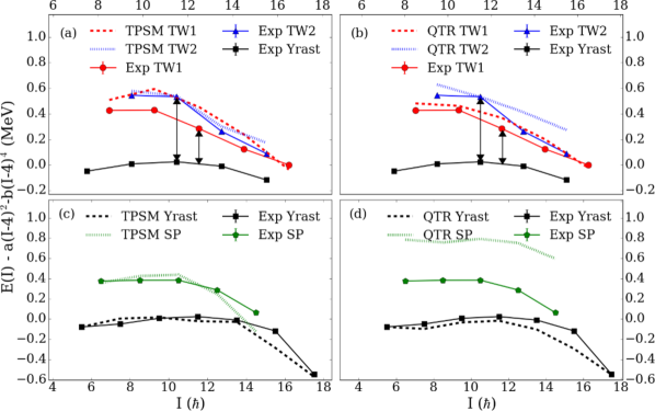
Figure 13: Experimental level energies minus a rotor contribution vs. spin, for the TW1, TW2, Yrast and SP bands in ¹³⁵Pr compared with the corresponding TPSM and QTR (labelled as QTR) calculations. The double pointed arrows between the experimental TW2, TW1 and Yrast points indicate the wobbling energy for the TW2 and the TW1 bands, respectively. Reproduced with permission from Ref. 135pr-2019PLB .

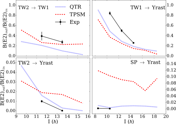
Figure 14: B(E2)${}_{\text{out}}$/B(E2)${}_{\text{in}}$ vs. spin for the TW2 $\rightarrow$ TW1, TW1 $\rightarrow$ Yrast, TW2 $\rightarrow$ Yrast and the SP $\rightarrow$ Yrast transitions. (TPSM (red dashed line), QTR (blue dotted line) and experiment (black squares connected by black solid line). Reproduced with permission from Ref. 135pr-2019PLB .

The calculations motivated U. Garg’s group to measure the mixing ratios of the $I\rightarrow I-1$ transitions between the suggested wobbling bands 135pr-2015PRL ; 135pr-2019PLB ; 135pr-erratum . Figs. 13 and 14 compare the results of the measurements with a slightly modified QTR calculation. As in Fig. 12, the excitation energy of the first (TW1) wobbling state decreases below and increases above $I_{c}$. The distance between TW1 and the second (TW2) wobbling state is much smaller than the excitation energy of TW1, which indicates strong anharmonicities. The ratios $\frac{B(E2,I\rightarrow I-1)_{out}}{B(E2,I\rightarrow I-2)_{in}}$ show the enhancement that signifies the collective nature of the wobbling mode. The ratios $\frac{B(E2,TW2\rightarrow TW1)}{B(E2,TW1\rightarrow yrast)}\sim 1$ indicate strong anharmonicities as well. The ratios $\frac{B(E2,TW2\rightarrow yrast)}{B(E2,TW1\rightarrow yrast)}<0.05$ are small as expected. The QTR calculations also describe the excitation of the odd particle, the signature partner (SP) band. As it should be, its $\frac{B(E2,I\rightarrow I-1)_{out}}{B(E2,I\rightarrow I-2)_{in}}$ ratios are very small like in the experiment. However, the QTR places the SP band at too high energy.

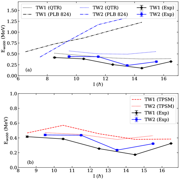
Figure 15: Wobbling energies $E_{W}(I)$ for ¹³⁵Pr compared with calculations. The labels TW1 and TW2 refer to the first and second band above the yrast band. QTR labels the calculations of Ref. 135pr-2019PLB , which uses fitted MoI’s. Ref. 135pr-Lv . PLB 824 labels the QTR calculations of Ref. 135pr-Lv , which used irrotational flow MoI. The pertaining calculated small ratios $\frac{B(E2,I\rightarrow I-1)_{out}}{B(E2,I\rightarrow I-2)_{in}}$ ratios indicate that TW1 has the character of a signature partner band. TPSM labels the triaxial projected shell model calculations from Ref. 135pr-2019PLB . Reproduced with permission from Ref. Sensharma2024 .

Lv et al. 135pr-Lv reinvestigated ¹³⁵Pr. In contrast to Refs. 135pr-2015PRL ; 135pr-2019PLB ; 135pr-erratum they determined small mixing ratios $|\delta|<1$, which indicate small $\frac{B(E2,I\rightarrow I-1)_{out}}{B(E2,I\rightarrow I-2)_{in}}$ ratios and large $\frac{B(M1,I\rightarrow I-1)_{out}}{B(E2,I\rightarrow I-2)_{in}}$ ratios. They presented the results as "Evidence against the wobbling nature of low-spin bands in ¹³⁵Pr", because large collective $E2$ transitions between the bands are the decisive signature for TW. In measuring the mixing ratios the challenge is to decide between the two minima of $\chi^{2}$ from the fit to the angular distributions. The authors of Ref. 135pr-Lv chose the minimum with small $|\delta|$ the authors of Refs. 135pr-2015PRL ; 135pr-2019PLB ; 135pr-erratum chose the one with large $|\delta|$. In Ref. Sensharma2024 Sensharma et al. present additional details of their fit procedure which support their choice of the large $|\delta|$.

The QTR calculations in Ref. 135pr-Lv account for the small $\frac{B(E2,I\rightarrow I-1)_{out}}{B(E2,I\rightarrow I-2)_{in}}$ ratios, which reassign the TW1 band as a signature partner band. The new assignment is supported by composition of the QTR states discussed in supplementary material of Ref. 135pr-Lv . The difference between the two QTR calculations consists in the inertia asymmetry, which is $\kappa=0.71$ for the fitted MoI’s of Refs. 135pr-2015PRL ; 135pr-2019PLB ; 135pr-erratum and $\kappa=-0.17$ for the irrotational-flow MoI’s of Ref. 135pr-Lv . The small $\kappa$ causes a very early instability of the TW regime which moves the SP band below the wobbling band. The SP band is characterized by the steady increase of $E_{W}(I)$ seen in the upper panel of Fig. 15.In my view, the stark contrast with the observed decrease $E_{W}(I)$ makes the SP assignment unbelievable. (Private communication of the QTR energies by E. Lawrie is acknowledged.)

The TSPM calculations (See Section V) in the lower panel of Fig. 13 evaluate the rotational response microscopically. There is no freedom in choosing the MoI’s. The similarity between the QTR of Refs. 135pr-2015PRL ; 135pr-2019PLB ; 135pr-erratum and the TSPM results lends credibility to the adjusted inertia asymmetry ratio of $\kappa=0.71$.

When the TW1 band were the SP band then it would be difficult to explain the presence of second nearby band with SP properties, which was observed in Refs. 135pr-2015PRL ; 135pr-2019PLB ; 135pr-erratum . Finally there is the far-reaching analogy between ¹³⁵Pr and ¹⁰⁵Pd (see next paragraph), for which the carefully measured mixing ratios indicate large $\frac{B(E2,I\rightarrow I-1)_{out}}{B(E2,I\rightarrow I-2)_{in}}$ ratios, which are consistent with the ones of Refs. 135pr-2015PRL ; 135pr-2019PLB ; 135pr-erratum .

In my opinion all the mentioned facts favor the TW interpretation of the bands. A new experiment would be needed to safely establish the experimental $\delta$ values.

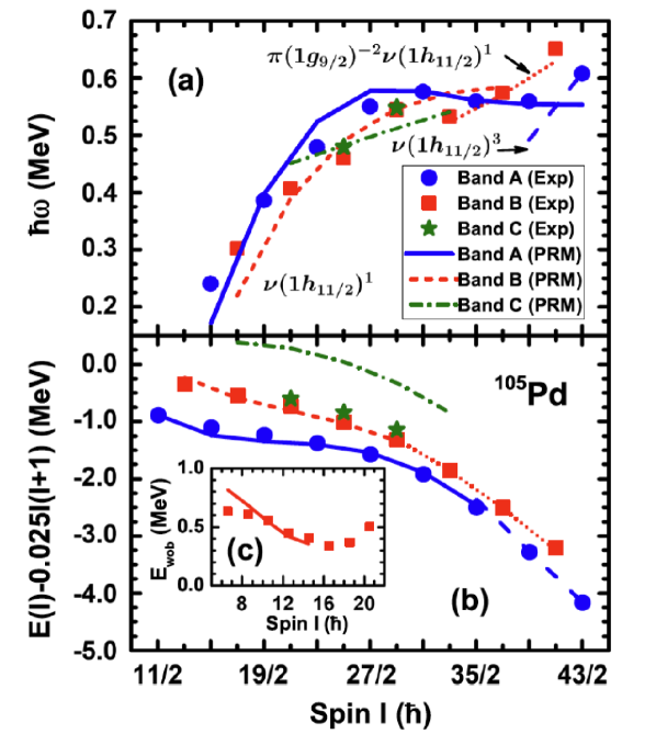
Figure 16: Experimental values derived from the energies of lowest bands in ¹⁰⁵Pd compared with the QTR (labelled as PRM) calculations: (a) rotational frequency, (b) energies minus a rotor reference with the wobbling energies $E_{W}(I)$ as the inset (c). The bands A, B and C are assigned to, respectively, $n=0$ TW, $n=1$ TW and SP. Reproduced with permission from Ref. Timar1 .

Another example for TW is ¹⁰⁵Pd, which was studied in Ref. Timar1 . The authors carried out QTR (called PRM) calculations using a triaxial deformation of $\gamma=25^{\circ}$ derived from mean field calculations and fitted MoI’s, which correspond to an inertia asymmetry of $\kappa=0.69$. Fig. 16 compares the experimental results with QTR calculations (denoted as PRM), where the rotational frequency is defined as

$$\hbar\omega(I-1/2)=(E(I)-E(I-2))/2.$$ (22)

The experimental (PRM) $\frac{B(E2,I\rightarrow I-1)_{out}}{B(E2,I\rightarrow I-2)_{in}}$ ratios for the $n=1\rightarrow 0$ trrasitions are $I=$17/2: 0.66$\pm$0.18 (0.736), $I=$21/2: 0.60 $\pm$0.09 (0.465), $I=$25/2: 0.34$\pm$ 0.07 (0.329).

From the PTR perspective the nucleus is much like ¹³⁵Pr, just that the odd $h_{11/2}$ proton is replaced by the odd $h_{11/2}$ neutron. The slightly lower inertia asymmetry as compared to ¹³⁵Pr is reflected by the somewhat higher value of $I_{c}=33/2$ of the minimum of the wobbling energy. The QTR predicts energy of the SP bands too high as in the case of ¹³⁵Pr.

A fourth band was reported in Ref. Timar2 . The experiment could not substantiate the nature of the band. Karmakar et al. Karmakar2024 measured mixing ratios for the transitions connecting it with the TW1 band, which did not indicate a strong $E2$ component. The finding is in contrast to ¹³⁵Pr where the connecting transitions of the analog band with TW1 show a strong $E2$ component, which allowed the authors of Ref. 135pr-2019PLB to identify it as the second wobbling excitation TW2. In ¹⁰⁵Pd band 4 represents a TW excitation on top of the SP band. The reason for the difference is the lower energy of the SP band in ¹⁰⁵Pd than in ¹³⁵Pr. As a consequence, in ¹⁰⁵Pd the TW excitation on the SP band has a smaller energy than the second wobbling excitation, while in ¹³⁵Pr the second wobbling excitation has a smaller energy than the TW excitation on the SP band. The microscopic TPSM calculations (See Section V.) account for the different nature of band 4, while the QPR predicts TW2 for band 4 in both nuclei. The latter is not surprising because the QTR overestimates the energy of the SP band in both nuclei.

Mukherjee et al. 151Eu identified in ¹⁵¹Eu a TW band built on the proton $h_{11/2}$ yrast band together with the pertaining SP band. See Section VI for an analysis in the framework of the TPSM.

Nandi et al. 183AuTW identified in ¹⁸³Au a TW band built on the proton $h_{9/2}$ band and another TW band built on the proton $i_{13/2}$ band. The wobbling energies from the $h_{9/2}$ pair decrease rapidly corresponding to a $I_{c}\approx 14$. The wobbling energies of the $i_{13/2}$ pair slowly increase like the PTR $E_{W}$ in Fig. 10 far below $I_{c}\approx 30$. The authors used different MoI’s to reproduce the different $I_{c}$ and the resulting $I$-dependences of $E_{W}(I)$, which also provided the correct $\frac{B(E2,I\rightarrow I-1)_{out}}{B(E2,I\rightarrow I-2)_{in}}$ ratios. Remarkably, the microscopic TPSM reproduces these quantities of both TW bands with nearly the same set of input deformations. See Fig. 12.11 and 12.14 of Chapter 12 and Fig. 14 of Ref. 151Eu .

Rojeeta Devi et al. 133BaTW confirmed the prediction Frauendorf2014PRC that TW appears for high-hole states as well, where the $\mathbf{J}$ precesses about the l-axis. They identified in ¹³³Ba the first and second TW bands built on the neutron $h_{11/2}$ hole band and carried out a qualitative analysis in HFA approximation.

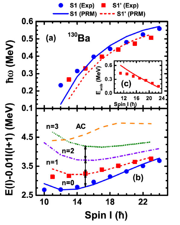
Figure 17: Experimental values derived from the energies of the bands S1, S1’ and AC in ¹³⁰Ba compared with the QTR (labelled as PRM) calculations: (a) rotational frequency, (b) energies minus a rotor reference with the wobbling energies $E_{W}(I)$ as the inset (c). The QTR calculations used the parameters $\varepsilon=0.24,~{}\gamma=21^{\circ},~{}{\cal J}_{s}/{\cal J}_{m}/{\cal J}_{l}=(0.73,1,0.43)\hbar^{2}$/MeV, respectively. Reproduced with permission from Ref. 130BaTW .

The TW regime is more stable when two particles align their angular momentum with the s-axis, as the value of $j$ in $I_{c}$ doubles. The first example of TW on a $\pi(h_{11/2})^{2}$ configuration was reported by Chen et al. 130BaTW for ¹³⁰Ba. The even-$I$ band S1, which is AB in CSM notation, was interpreted as the $n=0$ TW band. The odd-$I$ band S1’ was assigned to the $n=1$ TW band. The second odd-$I$ band, called AC in CSM notation, represents the SP band, because the quasiproton B is replaced by C with the opposite signature. They compared the experimental values with QTR (labelled as PRM) calculations using the deformation parameters from a mean field calculation and adjusting the MoI’s to fit the energies of the $n=0$ and 1 bands.

Fig. 17 compares the rotational frequencies and the energies of the bands S, S’ and AC with the PRM results, which agree rather well. The experimental mixing ratios of the $I\rightarrow I-1$ transitions between the $n=1$ and $n=0$ bands allowed the authors determining $\frac{B(E2,I\rightarrow I-1)_{out}}{B(E2,I\rightarrow I-2)_{in}}$ ratios between 0.3 and 0.4, which signify the wobbling character of the $n=1$ band. They are consistent with the PRM ratios $\frac{B(E2,I\rightarrow I-1)_{out}}{B(E2,I\rightarrow I-2)_{in}}$=0.51, 0.42, 0.35, 0.29, 0.25 for $I$=13, 17, 19, 21, respectively. The $E2$ component of the transition from the AC band to the $n=0$ (AB) band was found to be small as expected for the SP band.

The wobbling energy in Fig. 17 shows that that the TW regime is stable within the displayed spin range ($I_{c}$=37). Fig. 18 displays the SCS probability distributions for $I=14$ and 15. The $n=0$ and AC states correspond to uniform rotation about the s-axis. The $n=1$ and $n=2$ states show the precession orbits around the s-axis, which characterize the TW regime.

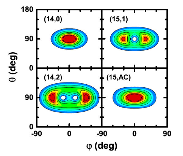
Figure 18: SCS probability distributions $P(\theta,\phi)$ of the angular momentum orientation $\mathbf{J}$ with respect to the body-fixed frame for the four lowest bands in Fig. 18. The color sequence with increasing probability is dark blue - green - dark brown. In accordance with Fig. 17, the panels are labeled by $(I,n)$ with $n$ being TW wobbling number or AC. Reproduced with permission from Ref. 130BaTW .

A second example for TW on the $\pi(h_{11/2})^{2}$ configuration is ¹³⁶Nd, which was studied by Chen and Petrache 136NdTW .

III.3 Transition from transverse to longitudinal wobbling in triaxial normal deformed nuclei

The FA approximation provides only a first qualitative TW-LW classification. The $\mathbf{j}$ of the odd particle reacts to wobbling motion of the nucleus, which must be taken into account to understand the region where the TW becomes unstable and beyond. For this purpose Chen and Frauendorf Chen_Frauendorf2022EPJA invoked the classical adiabatic energy. The classical energy is defined by replacing in the PTR Hamiltonian (12,13) the operators by their corresponding classical numbers,

$$\hat{J}_{3}\rightarrow J\cos\theta,~{}~{}\hat{J}_{1}\rightarrow J\sin\theta\cos\phi,~{}~{}\hat{J}_{2}\rightarrow J\sin\theta\sin\phi,$$ (23)

$$\hat{j}_{3}\rightarrow j\cos\vartheta,~{}~{}\hat{j}_{1}\rightarrow j\sin\vartheta\cos\varphi,~{}~{}\hat{j}_{2}\rightarrow j\sin\vartheta\sin\varphi.$$ (24)

The adiabatic classical energy $E_{ad}(\theta,\phi)$ is obtained by minimizing the classical energy $E_{class}(\theta,\phi,\vartheta,\varphi)$ with respect to $\vartheta$ and $\varphi$ for given $\theta,~{}\phi$, that is, let the particle react to the Coriolis force. It is displayed Fig. 19 for the PTR Hamiltonian of ¹³⁵Pr. The energy contours represent the classical orbits when $\mathbf{j}$ adiabatically follows $\mathbf{J}$, which is the case when the energy scale of the particle is large compared to the scale of the wobbling mode. As demonstrated in Ref. Chen_Frauendorf2024 , adiabticity is a reasonable approximation for the lowest three bands. See Figs. 24 and 29 below.

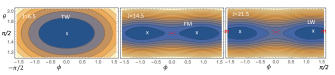
Figure 19: Adiabatic classical energy $E_{ad}(\theta,\phi)$ in ¹³⁵Pr for the TW, FM and LW regimes. The contours of constant energy represent the classical orbits with the corresponding energy and the indicated angular momentum. Minima are marked by white crosses and saddles by red crosses. The letters s and m indicate the location of the s-and m-axes.

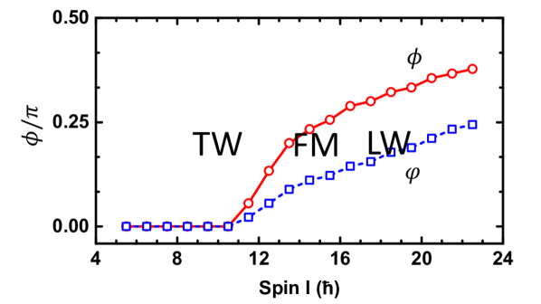
Figure 20: Location of the minima of the adiabatic classical energy $E_{ad}(\theta,\phi)$ in ¹³⁵Pr on the line $\phi=\pi/2$ in Fig. 19 (marked by the white crosses). The pertaining angles of $\mathbf{j}$ are $\vartheta=\pi/2$ and $\varphi$. Reproduced with permission and adapted from Ref. Chen_Frauendorf2022EPJA .

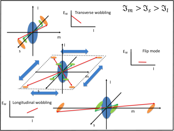
Figure 21: Schematic illustration of the collective wobbling modes. Green arrows show the precession cones of the particle $\mathbf{j}$ and red arrows the precession cones of the total angular momentum $\mathbf{J}$.

The $I$ dependence reflects the competition between the Coriolis force, which tries to keep the angle between $\mathbf{J}$ and $\mathbf{j}$ small, the triaxial potential, which tries to align $\mathbf{j}$ with the s-axis and the energetic preference of the m-axis with the maximal MoI. Fig. 20 shows the angles $\phi$ and $\varphi$ of the minimum of the adiabatic energy.

At low $I$ the classical orbits revolve the s-axis, which is the TW regime. At the critical angular momentum of $J_{c}=10.5$ the $\phi=0$ minimum changes into a maximum and two minima at $|\phi|>0$ emerge. The rotation about the s-axis becomes unstable. The TW regime changes into the flip mode (FM), which becomes well established at $J=14.5$. The FM represents flipping between the narrow precession cones around the two tilted axes. Quantum mechanically, the $n=0$ state is an even and the $n=1$ state an odd superposition of two states localized near the tilted axes. As the two minima at $\phi_{0}$ approach $\pm\pi/2$ the orbits merge with the ones at $\pi\mp\phi_{0}$ such that the precession cones revolve around the m-axis, which means the region of LW has been reached.

The flip regime appears around $I=14.5$ where $E_{W}$ has its minimum in Fig. 13. At larger $I$ values $E_{W}(I)$ increases with $I$. As seen in Fig. 20, the angle $\varphi$ of the particle $\mathbf{j}$ remains far below $\pi/2$ in this region. Therefore the authors of Ref. Chen_Frauendorf2022EPJA suggested a generalization of the TW-LW classification of Ref. Frauendorf2014PRC , which is based on the topology of the classical orbits that correspond to the quantal states:

Classification of the	$\mathbf{J}$ revolves	$\mathbf{j}$ revolves	$E_{W}(I)$	$\frac{B(E2,I\rightarrow I-1)_{out}}{B(E2,I\rightarrow I-2)_{in}}$
lowest bands	around axis	around axis
transverse wobbling (TW)	short or long	short or long	decreases∗	order one
longitudinal wobbling (LW)	medium	short, long, tilted	increases	order one
flip mode (FM)	tilted	tilted	constant	order one
signature partner (SP)	short, medium, long	short, medium, long	increases	small

^∗ Depending on $I_{C}$ there may be a slight increase at low $I$.

The scheme is quite simple from the experimental point of view and has been used in Refs. Frauendorf2014PRC ; 135pr-2015PRL ; 135pr-2019PLB in classifying the experimental results. Fig. 21 illustrates the angular momentum geometry in a schematic way.

The energy difference between the $n=0$ and $n=1$ states of the flip mode reflects the mixing of the states localized near the tilted axis. It disappears when the coupling goes to zero. This limit represents uniform rotation about a tilted axis, which breaks the signature symmetry and leads to a $\Delta I=1$ band (see discussion of the rotating mean field symmetries in Ref. SFrmp ).

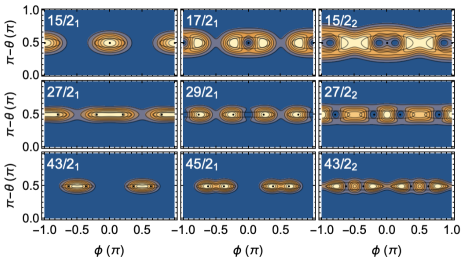
Figure 22: Probability distribution of the angular momentum orientation $P(\theta\phi)_{I\nu}$ generated from the reduced density matrix of the PTR calculation for ¹³⁵Pr in Ref. Frauendorf2014PRC . The three rows show the SCS maps for the TW, FM, and LW regimes. The black curves show the classical orbits obtained by setting the adiabatic classical energy equal to the quantal energy of the states. The author thanks Q. B. Chen for preparing the figure.

Fig. 22 shows the probability distribution of the $\mathbf{J}$ with respect to the principal axes for the lowest three bands $n=$0, 1, 2. The classical orbits (as shown in in Fig. 19) for the quantal energies of the states are included.

The SCS maps in the upper row show rims that are centered at the s-axis, which are the hallmark of TW.

The middle row shows the four spots near the tilted axes between the FM flips. The $27/2_{1}$ state represents the even superposition (large $P(0)$ and the $29/2_{1}$ state the odd superposition ($P(0)=0$) of the flip states. The $27/2_{2}$ state flips between the s- and m-axes, which are both unstable. The structure is analog to the flip mode of the unstable s-axis of the TR discussed in Sec. II.

The lower row displays the LW regime. The very elongated orbits enclose the m-axis at $\pm\pi/2$, which is the topological characteristics of LW. They differ substantially from the HFA-LW limit, because the minima of $E_{ad}$ are still away from the m-axis (see Fig. 20).

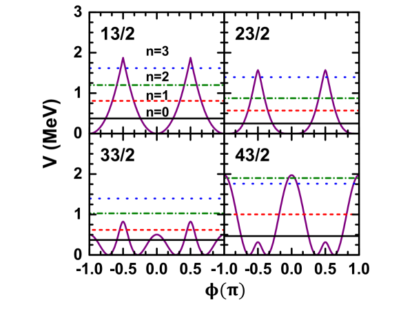
Figure 23: Classical adiabatic energy of ¹³⁵Pr $V(\phi)=E_{\textrm{ad}}(\pi/2,\phi)$ for selected spins. The horizontal lines show the PTR energies $E_{n}-E_{ad}(\phi_{0})$ relative to the minimum of $E_{ad}$ at $\phi_{0}$. For the two values of $n$ that do not appear for $I$ the line is located at $(E_{n}(I-1)+E_{n}(I+1))/2$. Reproduced with permission and adapted from Ref. Chen_Frauendorf2022EPJA .

Figure 24: Full curves show the probability density of the SSS for the $n$ = 0, 1, 2, 3 states calculated by PTR for ¹³⁵Pr, while the dashed curves display the ones from the collective Hamiltonian (CH). Reproduced with permission Ref. Chen_Frauendorf2024 .

For the classical TR the angular momentum component $J_{3}$ and the angle of $\mathbf{J}$ with the saxis in the s-m- axes plane represent the momentum and coordinate of a pair of canonical variables. This provides a complementary perspective on the structure of the PTR states. It employs the correspondence between the classical motion in a potential and the probability density of the corresponding quantal Hamiltonian, which is familiar from the textbooks. The classical adiabatic energy at $E_{ad}(\pi/2,\phi)$ represents the potential $V(\phi)$. For not too high energy one can expand the classical adiabatic energy up to second order in $\theta-\pi/2$, which gives the classical adiabatic Hamiltonian

$$H_{ad}=T+V(\phi),~{}~{}T=\frac{J_{3}^{2}}{2B(\phi)},~{}~{}\frac{1}{B(\phi)}=\frac{1}{I^{2}}\frac{\partial^{2}E_{ad}(\theta,\phi)}{\partial\theta^{2}}\Bigr{\rvert}_{\pi/2}.$$ (25)

The potential is shown in Fig. 23 together with bars at the PTR energies relative to the minimum of $V(\phi)$. The difference represents the kinetic energy T. If $T>0$ the wave function oscillates with a wavelength that decreases with $T$. If $T<0$ the wave function decreases exponentially with $|T|$. The value of $T$ defines the TW-FM-LW classification. In the TW regime ($I$=13/2, 23/2) the s-axis is in the range $T>0$, and in the LW regime ($I$=43/2) the m-axis is in the range $T>0$. In the FM the $n$ =0 and $n$=1 states are localized around $\phi\approx\pm\pi/4$. The mode flips between rotation about the two orientations of the tilted axis.

Chen and Frauendorf introduced the Spin Squeezed State (SSS) representation of the reduced density matrix Chen_Frauendorf2024 .

$$P(\phi)_{\nu}=\frac{1}{2\pi}\sum\limits_{K,K^{\prime}=-I}^{I}e^{-i(K-K^{\prime})\phi}\rho^{(\nu)}_{KK^{\prime}},$$ (26)

where $\phi$ is the angular momentum angle with the s-axis in the s-m-plane. The over-complete, non-orthogonal basis comes as close to a continuous wave function as possible for the finite Hilbert space of dimension $2I+1$. It is generated by rotating the localized state

$$|II0\rangle=(2I+1)^{-1/2}\sum\limits_{K=-I}^{I}|IIK\rangle$$ (27)

around the 3-axis. It has a smaller width of $\sim 3/2I$ as compared to the width $\sim 1/\sqrt{2I}$ of the generating state of the SCS basis. Fig. 24 shows the SSS plots of some states for ¹³⁵Pr, some of which are displayed in the form of SCS maps in Fig. 22.

The TW states $I<25/2$ have the profile of oscillations within the potential centered at the s -axis. The $n=0$ states have a maximum at $\phi=0$. The $n=1$ states have a minimum at $\phi=0$, and the $n=2$ states have two minima at $\phi=\pm\pi/6$. If the states were pure, the minima would be the zeros of the collective wave function that characterize the oscillations. There is a certain degree of incoherence caused by the deviations from the adiabatic approximation, which lead to a finite probability density at the minima (see discussion in Sec. III.5).

The LW states $I>37/2$ have the profile of oscillations within the potential centered at the m-axis: The $n=0$ states have maxima at $\phi=\pm\pi/2$. The $n=1$ states have minima at $\phi=\pm\pi/2$, and the $n=2$ states have two minima near $\phi=\pm 4/6\pi$.

The FM states around $I=31/2,~{}33/2$ have flip character. The $n=$0 and 1 are the respective even and odd linear combinations of the two states localized at $\phi\approx\pm\pi/4$. The $n=2$ states are standing waves with probability maxima at the the tops of the barriers where the classical motion is slowest.

The SSS curves are similar to the profile of the SCS maps along the line $\theta=\pi/2$. This reflects the fact that the SCS states along this path are generated by rotating the localized state $|IIK_{s}=I\rangle$ around the l-axis instead of the SSS basis state, (27), which is also centered at the s-axis just being more narrow. The over-completeness of the SCS and SSS basis sets results in a certain ambiguity in visualizing of the structure.

III.4 Longitudinal wobbling in triaxial normal deformed nuclei

Biswas et al. 133LaLW reported the first case of LW for ¹³³La based on their observation of large $\frac{B(E2,I\rightarrow I-1)_{out}}{B(E2,I\rightarrow I-2)_{in}}$ ratios and increasing wobbling energy. Following this, evidence for LW was reported for ¹⁸⁷Au by Sensharma et al. 187AuLW and ¹²⁷Xe127XeLW by Chakraborty et al..

Figure 25: Wobbling and SP band energies in ¹³³La and ¹³⁵Pr compared with QTR calculations. Reproduced with permission from Ref. 133LaLW .

The wobbling energies of ¹³³La in Fig. 25 increase with $I$, which is the hallmark of LW. Biswas et al. 133LaLW measured the mixing ratios and found that $\frac{B(E2,I\rightarrow I-1)_{out}}{B(E2,I\rightarrow I-2)_{in}}$ ratios were collectively enhanced. The right panel shows the isotone ¹³⁵Pr with the discussed TW behavior. As in both nuclei the proton occupies the bottom of the $h_{11/2}$ shell, TW ought to appear in ¹³³La. The authors of Ref. 133LaLW explained the appearance LW as follows. TW in ¹³⁵Pr is the result of ${\cal J}_{s}<{\cal J}_{m}$, which is seen as a rapid increase of the rotational frequency with $I$ along the yrast band. In ¹³³La a much slower increase is observed, which is caused by the gradual alignment of the angular momentum of a pair of positive parity protons with the s-axis. The difference ${\cal J}_{m}-{\cal J}_{s}(I)$ becomes quickly small, such that rotation about the 1-axis remains energetically favorable, and the wobbling energy increases with $I$. The authors identified the role of the proton pair by comparing with the rotational response of ¹³⁴Pr where the alignment of the proton pair is blocked. The QTR calculations in Fig. 25 were carried out in the framework of the quasiparticle-core-coupling model (see Sec. VI) using a TR core with the MoI’s ${\cal J}_{s}=(9.12+0.66~{}R)~{}\hbar^{2}/MeV$ for ¹³³La and ${\cal J}_{s}=(9.34+0.10~{}R)~{}\hbar^{2}/MeV$ for ¹³⁵Pr and for both nuclei ${\cal J}_{m}=21~{}\hbar^{2}/MeV$, ${\cal J}_{l}=4~{}\hbar^{2}/MeV$ and a coupling strength corresponding to $\varepsilon=0.16,~{}\gamma=26^{\circ}$.

The TPSM calculations (see Fig.40 in Sec. V) reproduce the change from TW to LW for, respectively, $Z=61,~{}59$ in the $N=74$ isotones using nearly the same triaxial mean field, which confirms the microscopic origin of the change. The energies of the $h_{11/2}$ bands in the $Z=57,~{}N=74$ isotone indicate TW again, which is reproduced by the TPSM. It would be interesting to substantiate this by measuring the mixing ratios.

Based on their highly collective $\frac{B(E2,I\rightarrow I-1)_{out}}{B(E2,I\rightarrow I-2)_{in}}$ ratios, Sensharma et al. 187AuLW assigned LW to the $h_{9/2}$ pair of bands. They carried out QTR calculations using irrotational-flow MoI’s with $\gamma=23^{\circ}$, which correspond to an asymmetry of $\kappa=0.37$ of the inertia ellipsoid. Good agreement with experimental energies and the $\frac{B(E2,I\rightarrow I-1)_{out}}{B(E2,I\rightarrow I-2)_{in}}$ ratios was obtained. The TPSM calculations in Chapter 12 (See Figs. 12.11 and 12.14.) also gave LW with $\frac{B(E2,I\rightarrow I-1)_{out}}{B(E2,I\rightarrow I-2)_{in}}$ ratios very close to the experimental ones reported by Sensharma et al. 187AuLW

Guo et al. 187Au-Guo challenged the LW assignment for ¹⁸⁷Au. They disagree with the authors of Ref. 187AuLW on which of the two minima of the $\chi^{2}$ fit should be accepted in determining the mixing ratios $\delta$. Guo et al. 187Au-Guo chose the one with small $|\delta|$ at variance with Sensharma et al. 187AuLW , who chose the one with large $|\delta|$. This led to small $\frac{B(E2,I\rightarrow I-1)_{out}}{B(E2,I\rightarrow I-2)_{in}}$ and large $\frac{B(M1,I\rightarrow I-1)_{out}}{B(E2,I\rightarrow I-2)_{in}}$ ratios, which indicate SP instead of LW for the excited band. Guo et al. 187Au-Guo carried out QTR calculations using irrotational-flow MoI’s with $\gamma=12^{\circ}$. The weak asymmetry of $\kappa=0.97$ of the inertia ellipsoid is the reason that their QTR calculations assigned a signature partner pair to the two $h_{9/2}$ bands in good agreement with the experimental results based their choice of $|\delta|$.

The authors of Ref. 187AuLW are preparing an extended publication of their experimental results, which will address the controversy. The relevant experimental information is already published in Ref. Sensharma_Theses . In my view, the TPSM calculations, for which the MoI’s cannot be adjusted to the data but are fixed by the microscopic structure, represent clear evidence that supports the LW assignment.

III.5 Approximate solutions of the PTR model

III.5.1 Frozen alignment approximation

Approximate solutions of the PTR problem have been constructed in order to elucidate the physics of the coupled system. The HFA approximation was introduced in Ref. Frauendorf2014PRC to define the TW-LW classification. Budaca Budaca18 (See chapter 13) extended the HFA beyond the critical angular momentum $I_{c}$, given by Eq. (21). Above $I_{c}$ the minimum of the FA energy lies at the finite angle

$$\cos\phi_{0}=\frac{2A_{1}j}{(2I-1)(A_{1}-A_{2})}$$ (28)

in the case that $\mathbf{j}$ is aligned with the 1-axis. (The alignment with other axes is discussed as well.) The yrast states correspond to uniform rotation about an axis tilted by $\phi_{0}$ into the 1-2-plane. The author applied the harmonic approximation with respect to the tilted axis and presented simple algebraic expressions for the energies and reduced $E2$ and $M1$ transition probabilities for $I>I_{c}$, which complement the ones of Ref. Frauendorf2014PRC . Fig. 26 shows the HFA wobbling energies for $j=11/2$ and several $\gamma$ values. At the critical angular momentum $I_{c}$ the wobbling energy turns zero and then increases, which is the hallmark of LW. The model fails near near the instability $I_{c}$. Above $I_{c}$ the ellipses around the axes with the tilt angles $\phi_{0}$ and $\pi-\phi_{0}$ soon overlap (see Fig. 19). It remains to be seen how well the harmonic wobbling excitations about a tilted axis describe the FW regime.

Figure 26: Wobbling energies in HFA approximation for different values of the triaxiality parameter $\gamma$. Reproduced with permission from Ref. Budaca18 .

Figure 27: Wobbling energy adjusted to the experimental energies of ¹³⁵Pr. Reproduced with permission from Ref. Budaca18 .

The model is a handy tool for a quick exploration of experimental results. The problems around $I_{c}$ may not not become too serious when the distance between the discrete $I$ points is large enough, like in the case of ¹³⁵Pr displayed in Fig. 27. The pertaining values of $\frac{B(E2,I\rightarrow I-1)_{out}}{B(E2,I\rightarrow I-2)_{in}}$ ratios of 0.2 - 0.3 deviate substantially from the experimental and QTR values but confirm the collective enhancement.

The model has three parameters: $\gamma$, which controls the ratios of the irrotational flow MoI’s, ${\cal J}_{0}$, which sets the scale of the rotational energies and $j$ the particle angular momentum aligned with one of the principal axes. The author assumes that $j$ remains frozen to the axis, which is not realistic as demonstrated by Fig. 20. This suggests considering a fixed angle of $\mathbf{j}$ with the 1-axis as another parameter. In Ref. Budaca23 the authors studied this generalization. Unfortunately, no algebraic expressions for a handy application are given. Their derivation appears straightforward. The only complication is the solution of the transcendental equation for the angle of the minimum of the classical energy, which could be tabulated or displayed.

III.5.2 Small amplitude approximation

Tanabe and Sugawara-Tanabe Tanabe-energy (See Chapter 4) developed an algebraic approximation to the PTR. They applied the Holstein-Primakoff boson expansion to both operators $\mathbf{\hat{J}}$ and $\mathbf{\hat{j}}$ and kept the terms up to forth order in the boson number. In second order the PTR Hamiltonian represents two coupled harmonic oscillators. The eigen modes are found by solving a biquadratic equation, which has a simple analytic solution. Analytic expressions for the energies and transition probabilities in terms of the three MoI’s and the strength $\kappa$ of the triaxial potential are given. The fourth-oder terms are taken into account by first order perturbation theory in the eigenmode basis. The expression for the additional terms are given as well but are rather complex. The bands can be classified by the oscillator quantum numbers of the two eigenmodes.

Without coupling, there is a pure $\mathbf{J}$ oscillation, which is the wobbling mode and a pure $\mathbf{j}$ oscillation, which is the cranking or SP mode. The coupling mixes the modes. In the TW regime the mixed modes retain their character as being predominantly wobbling or cranking, and the $n_{wobb}$ and $n_{crank}$ oscillator quantum numbers can be assigned to the bands. The HFA represent the limit of a very stiff (large $\kappa$) cranking mode. The harmonic approximation breaks down when the minimum of the classical adiabatic energy at the angles $\theta=\pi/2$ and $\phi=0$ changes into a maximum. This the angular momentum where the angle $\phi$ deviates from zero in Fig. 20.

The authors applied the model to the TSD wobbling bands in the Lu and Tm isotopes assuming rigid body MoI’s corresponding to the equilibrium deformation. As the respective ratios are similar to the ones in Ref. hamamoto2 comparable good agreement with the experimental $\frac{B(E2,I\rightarrow I-1)_{out}}{B(E2,I\rightarrow I-2)_{in}}$ and $\frac{M1,I\rightarrow I-1)_{out}}{B(E2,I\rightarrow I-2)_{in}}$ ratios was obtained. For rigid body MoI’s the short axis has the largest MoI. Because this implies LW, their wobbling energies increase with $I$. In order to remove the discrepancy with the observed decrease they made the scale of the MoI’s increasing with $I$ as

$${\cal J}_{0}(I)={\cal J}_{0}\frac{I-0.60}{I+23.5}.$$ (29)

They attributed this increase to a gradual decrease of the pair correlations along the bands. The TDS bands cover the range of $I=13/2-97/2$. The scaling gives ${\cal J}_{0}(97/2)/{\cal J}_{0}(13//2)=3.14$. However, the experimental ratio of ${\cal J}^{(1)}$ is 73/65=1.12 and of ${\cal J}^{(2)}$ is 60/70=1.16 Hagemann2004 . Obviously, the pairing hypothesis is not convincing. The experimental change of the MoI’s cannot revers the $I$ dependence of the wobbling energy. As discussed at the beginning of Section II, the rigid body MoI’s ratios contradict the general principle of spontaneous symmetry breaking. The conclusions have been discussed at the beginning of Sec. III.1.

In Ref. 135Pr-tanabe1 the authors applied the model to ¹³⁵Pr assuming irrotational flow MoI’s and a triaxialty parameter $\gamma=26^{\circ}$ as used in Ref. Frauendorf2014PRC . They found that the harmonic vibrations become unstable for $I>13/2$ and claimed that the TW mode does not appear. Their claim has been refuted by Frauendorf Frauendorf2018PRC (see also their reply in Ref. 135Pr-tanabe2 ) for the following reasons. As discussed in the beginning of Sec. III.2, the PTR calculation with irrotational flow MoI’s for $\gamma=26^{\circ}$ result in an early transition of the TW into the FM around $I=17/2$ (See Fig. 16 of Ref. Frauendorf2014PRC ). In the small-amplitude approximation the TW becomes unstable when the minimum of the classical energy at $\phi=0$ disappears. This happens at a smaller angular momentum than the transition to the FM in the exact PTR calculation. (Compare $J$=10.5 in Fig. 20 with $I=25/2$ in Fig. 15). Hence the very early instability of the TW mode found in Ref. 135Pr-tanabe1 results from the combination of using irrotational flow MoI’s with the near maximal inertia asymmetry of $\kappa=-0.17$ and the harmonic approximation. It cannot be used to question the existence of the TW mode in normally deformed triaxial nuclei.

Raduta et al. Raduta2017 ; Raduta2018 (See Chapter 8) re-expressed the PTR Hamiltonian in the basis of the SCS, which becomes a continuous function of two variables that represent a canonical pair of momentum and coordinate. They approximated the Hamiltonian by expanding it up to second order in momentum and coordinate and solved the pertaining eigenvalue problem on the classical and quantal level. In essence, the approach is the two-oscillator model of Ref. Tanabe-energy (no fourth order terms). The authors studied ^163,165,167Lu. They assumed the rigid-body ratios of the MoI’s for the equilibrium deformation and adjusted the scale of the MoI’s and the strength of the deformed potential to the observed energies of the TSD bands. As one can expect, the results were similar to the ones of Ref. Tanabe-energy . The model well describes the $\frac{B(E2,I\rightarrow I-1)_{out}}{B(E2,I\rightarrow I-2)_{in}}$ and $\frac{M1,I\rightarrow I-1)_{out}}{B(E2,I\rightarrow I-2)_{in}}$ ratios but gives wobbling energies which increase with $I$. Hence, my remarks to the work Tanabe-energy apply accordingly.

In Ref. Raduta2020 Raduta et al. suggested that the TSD2 band can be interpreted as uniform rotation about the s-axis like the TSD1 band, where in the former case the core angular momentum $R=$3, 5, 7, … and in the latter $R=$2, 4, 6, … In Eq. (25) of Ref. Raduta2020 , they assigned to both bands the energies $E_{classical}(I)+\hbar\omega_{W}(I)/2$ with $I=$13/2, 17/2, 21/2, …. for TSD1 and $I=$15/2, 19/2, 23/2, …. for TSD2. The two terms $E_{classical}(I)$ and $\hbar\omega_{W}(I)$, derived in Refs. Raduta2017 ; Raduta2018 , are smooth functions of $I$. Therefore the model merges the two bands into one $\Delta I=1$ sequence. In other words, the wobbling energies are zero in stark contrast to the experiment. (A plot of the published energies confirms this. Private communication of the accurate energies by A. A. Raduta is acknowledged.) In Ref. Raduta2021 Raduta et al. applied the same approach to ¹³⁵Pr with the modification assuming a fixed orientation of the particle’s $\mathbf{j}$, which gave zero wobbling energies as well. In my view, the characterization of the wobbling mode discussed in Refs. Raduta2020 ; Raduta2021 on the basis of this approach cannot be trusted.

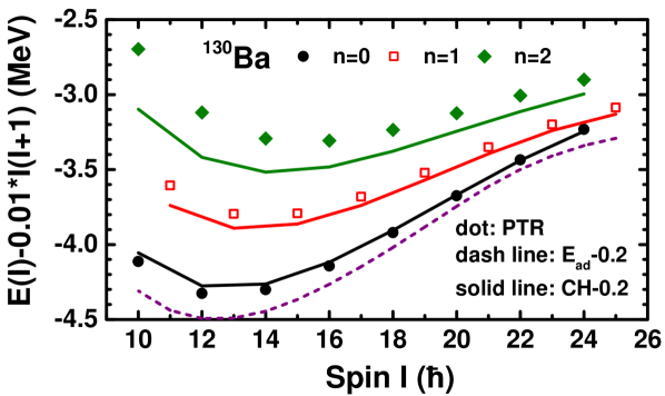
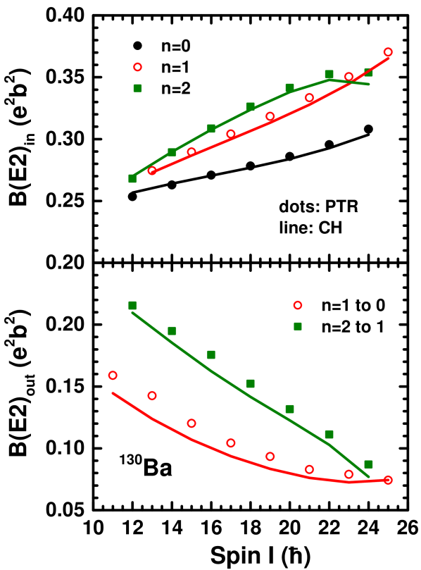
Figure 28: Comparison of the energies (left panel) and $B(E2)$ values (right panel) of ¹³⁰Ba calculated by means of the full PTR model (symbols) and the CH (solid curves). The adiabatic classic energy is shown by the dashed curve. All the energies are down shifted by 0.2 MeV. Reproduced with permission from Ref. Chen_Frauendorf2024 .

Figure 29: Full curves show the probability density of the SSS for the $n$ = 0, 1, 2, 3 states calculated by PTR for ¹³⁰Ba, while the dashed curves display the ones from the collective Hamiltonian (CH). Reproduced with permission from Ref. Chen_Frauendorf2024 .

III.5.3 Collective Hamiltonian

Frauendorf and Chen Chen_Frauendorf2024 quantized the classical adiabatic Hamiltonian (25) using the Pauli prescription for the replacing the classical kinetic energy $T$ by the corresponding operator $\hat{T}$. The resulting collective Hamiltonian (CH) was diagonalized in the basis of the axial rotor states $|IMK\rangle$. As the CH is invariant with respect to the $D_{2}$ group, all representations of the point group appear as eigenstates. Only the ones that are similar to the full PTR states are accepted.

Fig. 28 compares the energies and $B(E2)$ values calculated by means of the PTR and of the CH for ¹³⁰Ba. The CH reproduces the exact PTR values rather well. Fig. 29 compares the SSS plots generated from the reduced density matrices of the PTR solutions with the SSS plots generated from the corresponding eigenstates of the CH (c. f. Eq. (7). The CH densities for the $n=$0, and 1 states agree very well with the PTR densities. At the PTR minima, they become zero, which characterizes an oscillating pure wave function. The PTR density has only minima because the coupling to the two particles generates some degree of incoherence. The degree of incoherence increases with $n$, which is seen as a progressive washing out of the wave-function pattern. The pattern changes from the oscillations of the lowest Hermite polynomials in the harmonic TW region near $I$=10 to the onset of the flip regime near $I=$24.

For ¹³⁵Pr, the second example studied, the agreement of the observables between CH and PTR is comparable. As seen in Fig. 24, the incoherence increases more rapidly with $n$. This is expected, because one $h_{11/2}$ proton is weaker bound to the triaxial core than a pair of them. The $n=$0 and $n$=1 SSS-CH plots correlate very well with the SSS-PTR plots through the TW-FM-LW transition, which allows one to associate the structures with partially coherent quantum oscillations. For the states $n=2,~{}I\geq 39/2$ and $n=3$ the CH plots seriously deviate from the PTR plots, which indicates the break down of the adiabatic approximation.

There is no problem in generating the numerical solutions for the PTR Hamiltonian. There are several codes available, both with the reduced high-j and the full version the triaxial potential in the particle Hamiltonian $h_{p}$. One motivation to approximate the PTR model by a CH is the intuitive interpretation in terms of wave functions derived from a one-dimensional Hamiltonian of the form $T+V$. A second is that the study provides the proof of principle that one can construct a realistic CH Hamiltonian from the energy surface generated by a Tilted Axis Cranking calculation. The TAC approach is widely used for the interpretation of high-spin experiments. The TAC model accounts only for uniform rotation about the tilted axis, which defines the minimum of the energy. A CH constructed from microscopic TAC calculations will allow one to study excitations with wobbling nature in addition to the TAC solutions with $n$=0 nature. In the preceding work Chen2014 ; Chen2016 a CH was constructed with $V$ being the Routhian at a fixed rotational frequency and $T$ estimated by the HFA applied at the minimum of the Routhian, which also provided promising results. The feasibility of extending the TAC along this avenue should be investigated.

III.6 Virtues and limits of the PTR

The PTR model is simple from the conceptual point of view and has lead to the intuitive pictures of the underlying physics, which have been discussed so far. The computational effort is negligible. However there is the question of how to choose the input parameters. The triaxiality of the shape determines the potential that binds the particles to the rotor and the ratios between the MoI’s, the interplay of which produces the wobbling behavior. Microscopically the two elements are tied together. On the PTR level they are to some extend independent, which has the advantage to achieve a good description of the experiment by adjusting them. On the other hand, the freedom of the parameter choice may lead to qualitative different interpretations as discussed in the preceding sections. The parameter choice is restricted by the fundamental principle of spontaneous symmetry breaking, which requires the irrotatotional flow-like oder ${\cal J}_{l}<{\cal J}_{s}<{\cal J}_{m}$. The expressions (3) with the triaxility parameter $\gamma$ taken from some mean field calculations should be used with caution, because the equilibrium values usually represent the minimum of a shallow energy surface and often differ between various versions of the mean field approaches. The asymmetry parameter $\kappa$ of the MoI’s depends sensitively on $\gamma$ between $20^{\circ}$ and $30^{\circ}$ (see Fig. 2), which introduces an element of uncertainty. Adjusting the MoI’s to reproduce the energies of observed wobbling bands turned out to be the best strategy for interpreting specific experiments. (See also Chapter 10.)

In the microscopic approaches to be presented in the next two sections the deformed mean field determines both elements in a unique way, which reduces the number of parameters. In addition they avoid a basic problem of the PTR, which assumes that the collective orientation angles of the TR are completely independent of the particle degrees of freedom. Microscopic calculations by means of the cranking model show that this is only correct to some extend (See discussion in Section VI).

IV Random Phase Approximation

The microscopic descriptions of wobbling is based on the pairing-plus-quadrupole-quadrupole many-body Hamiltonian

$$\hat{H}_{PQQ} = \sum_{\tau=\pi,\nu}[\,\,\hat{h}^{\circ}_{\tau}-G_{\tau}(\hat{P}^{\dagger}_{\tau}\hat{P}_{\tau})-\lambda_{\tau}\hat{N}_{\tau}\,\,]$$ (30)

$$\quad\quad-\frac{\kappa_{{}_{0}}}{2}\sum_{m=-2,2}(-1)^{m}\hat{Q}_{m}\hat{Q}_{-m}.$$

The operator $\hat{h}^{\circ}_{\tau}$ is the spherical part of the Nilsson Hamiltonian, where the isospin index $\tau=\pi,\nu$ distinguishes the neutron and proton contributions, respectively, and $\hat{P}^{\dagger}_{\tau}$ and $\hat{P}_{\tau}$ are the familiar monopole pair operators. As pairing is treated in BCS approximation the terms $\lambda_{\tau}\hat{N}_{\tau}$, containing the particle number operators $\hat{N}_{\tau}$, are introduced to attain the average particle numbers. The following term in Eq. (30) is the quadrupole-quadrupole interaction, where $\hat{Q}_{m}=\sum_{\tau=\pi,\nu}\hat{Q}_{m}(\tau)$. The BCS approximation is applied to $H_{PQQ}$, which leads to the quasiparticle Hamiltonian

$$\hat{h}_{\tau}=\,\,\hat{h}^{\circ}_{\tau}-\Delta_{\tau}(\hat{P}^{\dagger}_{\tau}+\hat{P}_{\tau})-\lambda_{\tau}\hat{N}_{\tau}\qquad\qquad\qquad\qquad$$

$$-\,\hbar\omega_{{}_{0}}\frac{2}{3}\,\varepsilon\,\left(\,\cos{\gamma}\hat{Q}_{{}_{0}}-\frac{\sin{\gamma}}{\sqrt{2}}(\hat{Q}_{{}_{2}}+\hat{Q}_{{}_{-2}})\,\right).\quad$$ (31)

and the selfconsistency relations

$$\kappa_{{}_{0}}\langle\hat{Q}_{{}_{0}}\rangle=\quad 2/3\,\hbar\omega_{{}_{0}}\,\varepsilon\cos{\gamma},$$

$$G_{\tau}\langle P^{\dagger}_{\tau}\rangle=\Delta_{\tau},~{}~{}~{}~{}~{}\langle\hat{N}_{\tau}\rangle=N_{\tau},$$ (32)

where $\hbar\omega_{{}_{0}}=41A^{-1/3}$ MeV. The average $\langle...\rangle$ is taken with the quasiparticle configuration of interest. In the applications the deformation parameters $\varepsilon$, $\gamma$ and the pairing gaps $\Delta_{\tau}$ are taken as input, which fix by the relations (IV) the coupling constants $\kappa_{0}$ and $G_{\tau}$. The last equation is fulfilled by the appropriate choice of the Fermi energy $\lambda_{\tau}$.

Figure 30: Wobbling energies in RPA approximation for ¹⁶³Lu. The opening angle ot the precession cone around the s-axis is $\theta_{wob}$ with the scale (in degree) on the right axis. Reproduced with permission from Ref. Matsuzaki2002 .

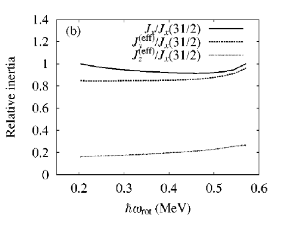
Figure 31: The moments of inertia (36) in RPA approximation for ¹⁶³Lu. The labels x, y, z correspond to 1, 2, 3. Reproduced with permission from Ref. Matsuzaki2002 .

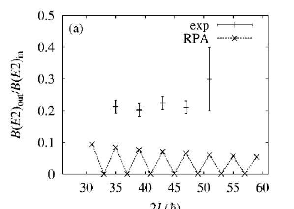
Figure 32: The $\frac{B(E2,I\rightarrow I-1)_{out}}{B(E2,I\rightarrow I-2)_{in}}$ ratios in RPA approximation for ¹⁶³Lu. Reproduced with permission from Ref. Matsuzaki2002 .

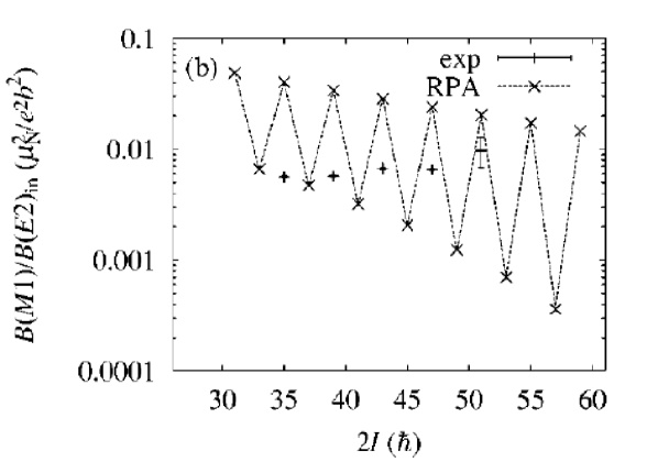
Figure 33: The $\frac{B(M1,I\rightarrow I-1)_{out}}{BE2,I\rightarrow I-2)_{in}}$ ratios in RPA approximation for ¹⁶³Lu. Reproduced with permission from Ref. Matsuzaki2002 .

The random phase approximation (RPA) to the wobbling mode has been developed by Michailov and Janssen MichailovRPAwobb ; JanssenRPAwobb and Marshalek Marshalek!979 . For the TW regime the RPA starts with finding the mean field solutions to the TAC Routhian

$$\hat{H}^{\prime}_{PQQ}=\hat{H}_{PQQ}-{\omega_{1}}{\hat{J}_{1}}-{\omega_{2}}{\hat{J}_{2}}-{\omega_{3}}{\hat{J}_{3}},$$ (33)

with $\omega_{1}=\omega_{rot},~{}\omega_{2}=\omega_{3}=0$. The solution represent uniform rotation about the s-axis, which is the yrast band, where the rotational frequency is chosen such $\langle J_{1}\rangle=I+1/2$. The solutions are given as configurations of quasiparticles generated by the quasiparticle Routhian

$$\hat{h}_{\tau}^{\prime}=\hat{h_{\tau}}-{\omega_{rot}}{\hat{J}_{1}},~{}~{}~{}[\hat{h}_{\tau}^{\prime},\alpha^{\dagger}_{m}]=E^{\prime}_{m}\alpha^{\dagger}_{m},$$ (34)

where $E^{\prime}_{k}$ are the quasiparticle energies in the rotating frame (quasiparticle routhians) and $\alpha^{\dagger}_{m}$ the pertaining quasiparticle creation operators. (For details of the TAC approach see e .g. Ref. SFrmp .)

Then it is assumed that $\omega_{2}(t)$ and $\omega_{3}(t)$ execute small harmonic oscillations, the wobbling mode. The solutions are found in first order of time-dependent perturbation theory. The wobbling frequency is given by the expression

$$\omega_{W}=\omega_{rot}\left[\frac{({\cal J}_{1}-{\cal J}_{2}(\omega_{w})({\cal J}_{1}-{\cal J}_{3}(\omega_{w})}{{\cal J}_{2}(\omega_{w}){\cal J}_{3}(\omega_{w})}\right]^{1/2},$$ (35)

which has the form of the original expression (10) from Ref. BMII . The expressions for the transition propabilities are the same as well. The microscopic MoI’s are similar to the ones from the cranking model

$${\cal J}_{1}=\frac{\langle J_{1}\rangle}{\omega_{rot}},~{}~{}~{}{\cal J}_{i=2,3}=4\sum_{k,m}\frac{|\langle|J_{1}\alpha^{\dagger}_{k}\alpha^{\dagger}_{m}|\rangle|^{2}(E^{\prime}_{k}+E^{\prime}_{m})}{(E^{\prime}_{k}+E^{\prime}_{m})^{2}-\omega_{W}^{2}},$$ (36)

where the indices $k,~{}m$ run over all quasiparticle excitations of the yrast configuration $|\rangle$. As both sides depend on $\omega_{W}$, Eq. (36) is the RPA dispersion relation, which must be solved numerically.

Matsuzaki et al. Matsuzaki2002 ; Matsuzaki2004 applied the method to the wobbling mode in ^163,167Lu. They used the deformation $\varepsilon=0.43,~{}\gamma=20^{\circ}$ and weak pairing of $\Delta_{n}=\Delta_{p}=0.3$ MeV. The one-quasineutron configuration $\alpha^{\dagger}_{i_{13/2}}|0\rangle$ was the yrast band, which implies the replacement $E_{m}\rightarrow-E_{m},~{}\alpha^{\dagger}_{m}\rightarrow\alpha_{m}$ for $m=i_{13/2}$ in the sum (36). Their results are compared with the experimental ones in Figs. 30 - 33.

As the wobbling energies are constant with a slight downward trend and the $\frac{B(E2,I\rightarrow I-1)_{out}}{B(E2,I\rightarrow I-2)_{in}}$ ratios are collectively enhanced, the results represent the first example for a microscopic description of TW. The authors explained the angular momentum dependence of $E_{(}I)$ in the same way as Frauendorf and Dönau when they introduced the TW-LW classification based on the HFA approximation Frauendorf2014PRC . The linear increase $\propto\omega_{rot}$ is overcompensated by the decrease of the factor ${\cal J}_{1}-{\cal J}_{2}$ in Eq. (35), which is caused by the decrease of ${\cal J}_{1}$. The origin of the latter is the presence of the particle’s $\mathbf{j}$ being aligned with the s -axis. In such a case the angular momentum $J_{1}=j+\omega_{rot}{\cal J}_{1}^{(2)}$ and $\bar{\cal J}_{1}=J_{1}/\omega_{rot}={\cal J}_{1}^{(2)}/(1-j/J_{1})$, which agrees with the $\bar{A}_{1}$ in Eq. (III.1). Assuming that $j=13/2$, one can estimate from the value of ${\cal J}_{1}$ in Fig. 31 that the TR MoI is ${\cal J}_{1}^{(2)}=0.67$ in the units of the figure at $\hbar\omega_{rot}$=0.2 MeV. The RPA calculations confirm the qualitative requirement ${\cal J}_{m}>{\cal J}_{s}>{\cal J}_{l}$ in a quantitative way.

Compared with the experiment, the wobbling energy is too small at low angular momentum and stays almost constant. The $\frac{B(E2,I\rightarrow I-1)_{out}}{B(E2,I\rightarrow I-2)_{in}}$ are by a factor of two too small and the $\frac{B(M1,I\rightarrow I-1)_{out}}{B(E2,I\rightarrow I-2)_{in}}$ ratios by a factor 5 - 10 too large.

The wobbling motion represent oscillations of $\mathbf{J}$ with respect to the principal axes of the triaxial shape. In the laboratory frame $\mathbf{J}$ stands still, and the triaxial shape oscillates. For small amplitudes wobbling is a harmonic oscillation of the mass quadrupole moment $Q_{1-}(t)=(Q_{1}(t)-Q_{-1}(t))/\sqrt{2}$. Application of the time-dependent perturbation theory leads to the well known RPA for separable interactions, which is equivalent with the just discussed RPA in the principal axes system Marshalek!979 .

In Ref. Frauendorf2015RPA Frauendorf and Dönau re-investigated ¹⁶³Lu by means of the standard RPA, because the available computer code allowed them to include other separable interactions. They kept $\kappa_{{}_{0}}$ constant and adjusted it to obtain $\varepsilon\approx 0.4$ over the range of $\omega_{rot}$, which gave $\gamma\approx 10^{\circ}$ from the self-consistency condition for $Q_{2}$. Weak pairing gaps of $\Delta_{n}=0.35,~{}\Delta_{p}=0.45$ MeV and standard effective charges of $e_{p}=e(1+Z/A)$ and $e_{n}=eZ/A$ charges were used. The results are labelled as $\mathrm{QQ}_{\mathrm{sc}}$ in Figs. 34 and 35. The results are quite similar to the ones of Matzusaki et. al. with the exception that the wobbling mode becomes unstable around $\hbar\omega=0.45$ MeV.

Using the deformations $\varepsilon\approx 0.4$ and $\gamma\approx 20^{\circ}$ from Matzusaki et al. marginally changed the results. Including the isovector $QQ$ and spin-spin interactions changed the results insignificately. However a current-current interaction of the type $\mathbf{L}\cdot\mathbf{L}$ did. As displayed by the curves $\mathrm{QQ}_{\mathrm{sc}}+\mathrm{LL}$ in Figs. 34 and 35, the wobbling energies agree very well with the experimental values, and the $\frac{B(M1,I\rightarrow I-1)_{out}}{BE2,I\rightarrow I-2)_{in}}$ ratios are reduced to the observed ones, while the $\frac{B(E2,I\rightarrow I-1)_{out}}{BE2,I\rightarrow I-2)_{in}}$ ratios did not change much.

The $\mathrm{LL}$ interaction couples the wobbling mode to the scissors mode, which is the isovector version of the wobbling mode: the proton system and the neutron system precess with anti-phase around the total angular momentum $\mathbf{J}$. The RPA calculation for the neighbor ¹⁶⁴Yb with the same coupling strength give the position and $B(M1)$ strength observed for the scissors mode in the nuclei of the region. A more detailed investigation of the relation between the scissors and wobbling modes seems interesting because the PTR calculations systematically overestimate the $\frac{B(M1,I\rightarrow I-1)_{out}}{BE2,I\rightarrow I-2)_{in}}$ ratios.

Figure 34: Wobbling energies in RPA approximation for ¹⁶³Lu. Reproduced with permission from Ref. Frauendorf2015RPA .

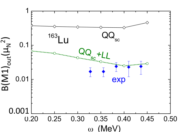
Figure 35: The $\frac{B(M1,I\rightarrow I-1)_{out}}{BE2,I\rightarrow I-2)_{in}}$ ratios in RPA approximation for ¹⁶³Lu. Reproduced with permission from Ref. Frauendorf2015RPA .

V Triaxial projected shell model

The triaxial projected shell model (TPSM) tpsm has been the other microscopic approach for studying the wobbling mode. More details are presented in chapters 12 and 14. The TPSM diagonalizes the pairing-plus-quadrupole-quadrupole many-body Hamiltonian (30) (augmented by a quadrupole pairing interaction) in the basis of quasiparticle configurations which are projected onto good angular momentum,

$$\hat{P}^{I}_{MK}\left|0\right>, \hat{P}^{I}_{MK}~{}a^{\dagger}_{p_{1}}\left|0\right>,$$

$$\hat{P}^{I}_{MK}~{}a^{\dagger}_{p_{1}}a^{\dagger}_{p_{2}}\left|0\right>, \hat{P}^{I}_{MK}~{}a^{\dagger}_{n_{1}}\left|0\right>,$$

$$\hat{P}^{I}_{MK}~{}a^{\dagger}_{n_{1}}a^{\dagger}_{n_{2}}\left|0\right>, \hat{P}^{I}_{MK}~{}a^{\dagger}_{p_{1}}a^{\dagger}_{n_{1}}a^{\dagger}_{n_{2}}\left|0\right>,$$

$$\hat{P}^{I}_{MK}~{}a^{\dagger}_{p_{1}}a^{\dagger}_{p_{2}}a^{\dagger}_{n_{1}}a^{\dagger}_{n_{2}}\left|0\right>, \hat{P}^{I}_{MK}~{}a^{\dagger}_{n_{1}}a^{\dagger}_{p_{1}}a^{\dagger}_{p_{2}}\left|0\right>,$$

$$..... \hat{P}^{I}_{MK}~{}a^{\dagger}_{p_{1}}a^{\dagger}_{p_{2}}a^{\dagger}_{p_{3}}a^{\dagger}_{n_{1}}a^{\dagger}_{n_{2}}\left|0\right>,$$ (37)

$$\hat{P}^{I}_{MK}~{}a^{\dagger}_{n_{1}}a^{\dagger}_{n_{2}}a^{\dagger}_{n_{3}}a^{\dagger}_{p_{1}}a^{\dagger}_{p_{2}}\left|0\right>,$$

$$.....$$

where $\left|0\right>$ represents the triaxial quasiparticle vacuum state, and $\hat{P}^{I}_{MK}$ projects the quasiparticle configuration on to good angular momentum states $|IMK\rangle$. In the majority of the nuclei, the near-yrast spectroscopy up to I=20 is well described using the above basis space. The extension is straight forward.

The input parameters are the pairing gaps and the deformation parameters $\varepsilon,~{}\varepsilon^{\prime}=\varepsilon\tan\gamma$. The PQQ coupling constants are fixed by means of the selfconsistency relations (IV). Usually $\varepsilon$ is taken from experiment or a mean field calculation and $\varepsilon^{\prime}$ is adjusted to the experimental band energies.

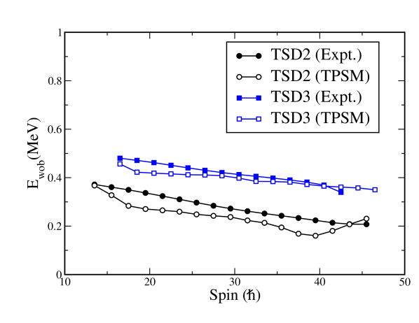
Figure 36: Wobbling energies in TPSM approximation for ¹⁶³Lu. From chapter 12, private communication by G. Bhat is acknowledged.

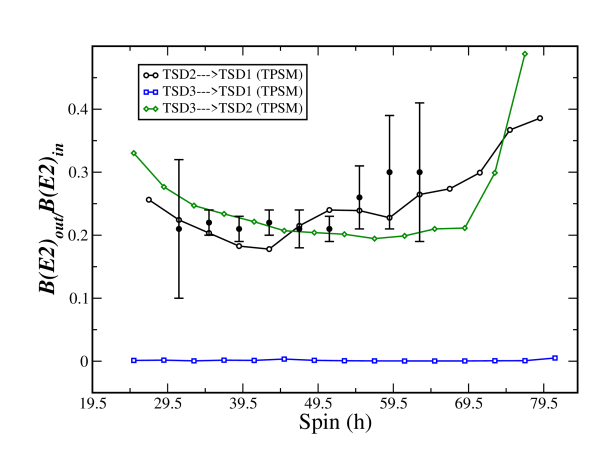
Figure 37: The $\frac{B(E2,I\rightarrow I-1)_{out}}{BE2,I\rightarrow I-2)_{in}}$ ratios in TPSM approximation for ¹⁶³Lu. From chapter 12, private communication by G. Bhat is acknowledged.

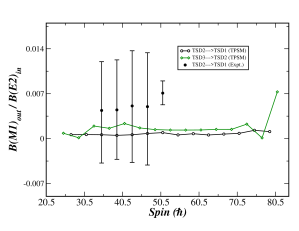
Figure 38: The $\frac{B(M1,I\rightarrow I-1)_{out}}{BE2,I\rightarrow I-2)_{in}}$ ratios in TPSM approximation for ¹⁶³Lu. From chapter 12, private communication by G. Bhat is acknowledged.

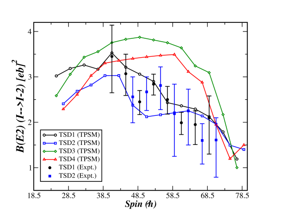
Figure 39: Intra band $BE2,I\rightarrow I-2)_{in}$ values in TPSM approximation for ¹⁶³Lu. From chapter 12, private communication by G. Bhat is acknowledged.

Sheikh presents of the systematics of theTPSM results for wobbling in chapter 12. I discuss only few examples which demonstrate the new aspects of the microscopic TPSM as compared to the semi-phenomenological PTR approach.

Sheikh and coworkers studied wobbling in the ¹⁶³Lu and the other Lu isotopes. (See chapter 12.) They used $\Delta_{n}=0.7527$ MeV, $\Delta_{p}=0.9637$ MeV and $\varepsilon=0.40$ and $\gamma=15^{\circ}$, which was adjusted to the experimental value of $E_{W}(21/2)$. The results displayed in Figs. 36 - 39 agree very well with the experimental data. The bands TSD1, TSD2, TSD3 are assigned to the bands with $n$=0, 1, 2 wobbling quanta. The band TSD4 contains the $h_{9/2}$ proton. The close-to-harmonic TW picture is substantiated. The wobbling energy decreases with the correct average slope. There are wiggles not seen in experiment. The $\frac{B(E2,I\rightarrow I-1)_{out}}{BE2,I\rightarrow I-2)_{in}}$ ratios for the $n\rightarrow n-1$ transitions show the collective enhancement of collective wobbling. The transition $n=2\rightarrow 1$ is suppressed.

Remarkably, the $\frac{B(M1,I\rightarrow I-1)_{out}}{BE2,I\rightarrow I-2)_{in}}$ ratios in Fig. 38 agree with the experimental values. These ratios are systematically overestimated in the PTR calculations. As discussed in Sec. IV, this also the case for the RPA calculations. Only the inclusion of the coupling to the scissors mode coupling reduced the ratios to their experimental values. It would be interesting to see if there is a connection between coupling to the scissors mode and the mutli-quasiparticle states of the TPSM basis (V), which include scissors configurations.

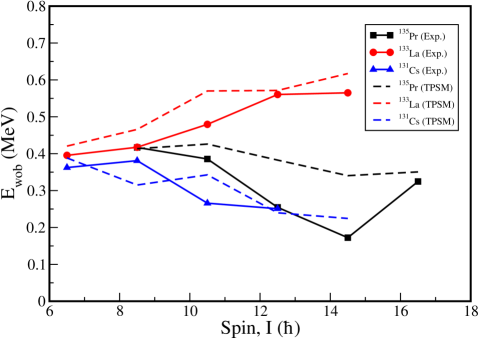
Figure 40: Wobbling energies in TPSM approximation for ¹³¹Cs, ¹³³La, ¹³⁵Pr. From chapter 12, private communication by G. Bhat is acknowledged.

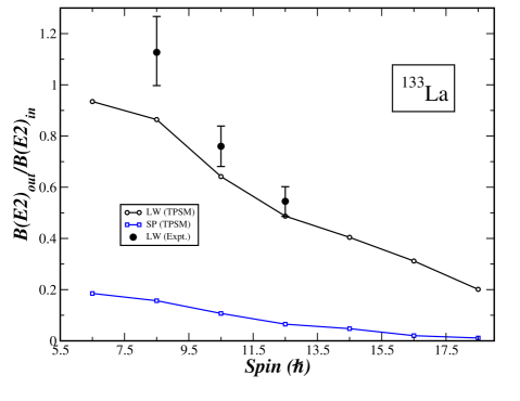
Figure 41: The $\frac{B(E2,I\rightarrow I-1)_{out}}{BE2,I\rightarrow I-2)_{in}}$ ratios in TPSM approximation for ¹³³La. From chapter 12, private communication by G. Bhat is acknowledged.

Fig. 40 compares the experimental wobbling energies of the three $N=74$ isotones $Z=$57, 59, 41 with the TPSM calculations, which used, respectively, $\varepsilon=$0.14, 0.15, 0.16 and $\varepsilon^{\prime}$=0.10 (corresponding to $\gamma=35^{\circ},~{}33^{\circ},~{}32^{\circ}$) as input. The fact that the TPSM with nearly constant $\varepsilon,~{}\varepsilon^{\prime}$ accounts for the observed TW-LW-TW sequence along the isotone chain indicates that the change originates from the change of the quasiparticle orbitals at the Fermi level. The details are discussed in Sec. III.2. Fig. 41 and 14 demonstrate the collective enhancement of the $n\rightarrow n-1$ transitions between the wobbling band in ¹³³La and ¹³⁵Pr, respectively.

Figs. 25 displays two examples for a general problem: The QTR predicts the SP band too high when locating the wobbling bands at the experimental energies. As seen in Fig. 13, TPSM locates both the SP and wobbling bands close to their experimental positions. The treatment of the TR core and the of the odd proton on equal footing in the microscopic TPSM seems to be decisive.

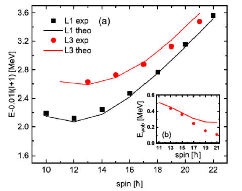
Figure 42: Energies in TPSM approximation for the $n$=0 (L1) and $n$=1 (L3) TW candidate bands in ¹³⁶Nd. The inset shows the wobbling energies. Reproduced with permission from Ref Fang-Petrache2021 .

Figure 43: SCS probability distributions for ¹³⁶Nd. Reproduced with permission and selected from Fig. 3 of Ref. Fang-Petrache2021 .

Chen and Petrache Fang-Petrache2021 (See chapter 14.) carried out TPSM calculation for the two-quasiproton configuration $(h_{11/2})^{2}$ in ¹³⁶Nd. Fig. 42 compare the TPSM energies with the ones of bands L1 and L3, which are interpreted as the $n$=0 and $n$=1 TW bands. Fig. 43 displays a selection of the SCS probability distributions generated from their TPSM results. For $I=10$ one sees the $n$=0 characteristics: uniform rotation around the s-axis and the ground state fluctuations around it. For $I=11$ the precession cone enclosing the s-axis is seen as the elliptical rim around it, which characterizes the $n$=1 TW state. The $I$=16 state is topologically classified as $n=0$ with large fluctuations in direction of the m-axis. The $I$=17 state is topologically classified as a strongly perturbed $n=1$ TW excitation. It encloses the s-axis, where the probability around $\phi=0$ is strongly reduced. The approach of the FM is apparent in form of the two maxima at $\phi=\pm 50^{\circ}$. The $I$=20 state has the characteristics of the $n=$0 FM. It flips between $-120^{\circ},~{}-60^{\circ},~{}60^{\circ},~{}120^{\circ}$ with no phase change, which indicated by the finite probability densities between the blops. The relatively large probabilities at $\phi=\pm 90^{\circ}$ herald the transition to the LW regime. The $I=21$ state has the characteristics of the $n=1$ FM with phase change between the flips. The approach of the LW mode is not apparent, because the symmetry requires $P(\theta=90^{\circ},~{}\phi=\pm 90^{\circ})=0$.

VI Soft core

In even-even nuclei triaxiality is indicated by the low energy ratio $E(2^{+}_{2})/$E($4^{+}_{!})$ ratio and the splitting between the even- and odd- spin members of the quasi $\gamma$ band. A staggering parameter

$$S(I)=\frac{[E(I)-E(I-1)]-[E(I-1)-E(I-2)]}{E(2^{+}_{1})}~{}~{}~{}~{}.$$ (38)

is defined, which measures the relative distance of the even- and odd-spin branches. When $S(I)$ is negative for even $I$ the even-$I$ sequence is lower than the odd-$I$ one. Then the nucleus is classified as "$\gamma$-soft", i. e. the triaxiality appears as a large-amplitude oscillation around around a near-axial shape. When $S(I)$ is negative for odd $I$ the odd-$I$ sequence is lower than the even-$I$ one. Then the nucleus is classified as "$\gamma$-rigid, i. e. the shape does not fluctuate much around some finite value of $\gamma_{)}$. The aspects of $\gamma$-softness are reviewed Ref. Frauendorf15 and discussed in detail in Ref. Rouoof2024 .

Most even-even nuclei with a low ratio of $E(2^{+}_{2})/$E($4^{+}_{!})$ are $\gamma$-soft. The few $\gamma$-rigid cases include the examples for wobbling discussed in Sec. II. In these cases $S(I)$ is equal to two times the difference between the single and double wobbling bands divided by the energy of the 2${}^{+}_{1}$ state. The TPR describes wobbling by coupling a rigid TR with one or two excited quasiparticles. This is in contrast with the observation that the "experimental cores", i. e. the $\gamma$ bands of the even-even neighbors (or the same nucleus), are $\gamma$-soft. Already Meyer-ter-Vehn was surprised how well his model applied to soft nuclei MtV1975 .

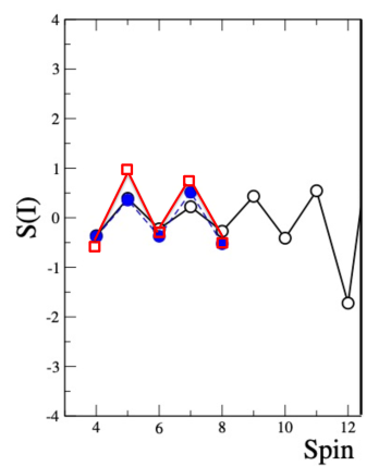
Figure 44: Staggering parameter for ¹³⁴Ce. Blue circles: experiment, red squares: Bohr Hamiltonian, black circles: TPSM - Private com. by G. Bhat acknowledged.

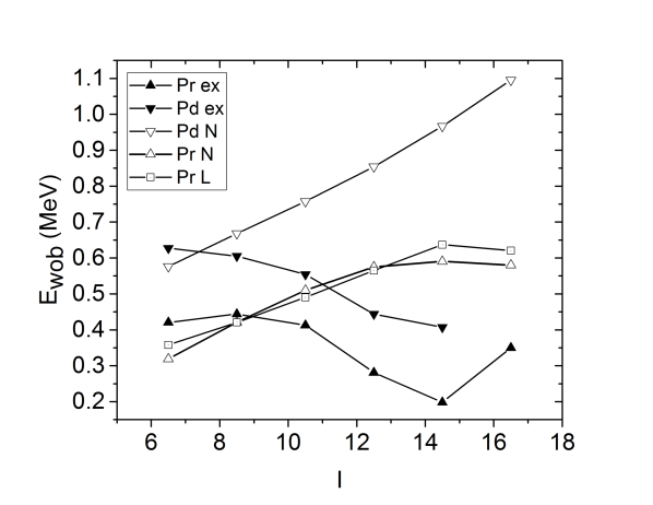
Figure 45: Wobbling energies from $\gamma$-soft cores for ¹³⁵Pr (Pr) and ¹⁰⁵Pd (pd) calculated by the model of Ref. Li-thesis (L) and the model of Ref. nomura-petrache (N) compared with the experiment (ex).

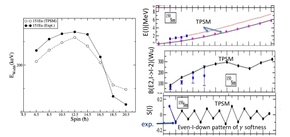
Figure 46: Left panel: Wobbling energies for ¹⁵¹Eu calculated by TPSM compared with the experiment 151Eu . Right panel: energies, $B(E2)_{in}$ values and staggering parameter of ¹⁵⁰Sm calculated by the TPSM compared with the experiment (blue dots and squares) Tab2018 . Reproduced with permission from Refs. 151Eu ; Tab2018

For this reason Li and advisors Li-thesis ; Li2022 used the core-quasiparticle-coupling model CQPCM for studying the coupling of a high-j quasiparticle to the soft core of Ref. MC11 , which incorporates the fluctuations of the $\gamma$ degree of freedom. The core is a simplified version of the Bohr Hamiltonian, the parameters of which were adjusted to the energies of the lowest collective states in ¹³⁴Ce. (See also Chapter 17.) Fig. 44 shows that the fitted Bohr Hamiltonian well approximates the $\gamma$-soft even-$I$-down pattern seen in ¹³⁴Ce. The resulting wobbling energies of the coupled system ¹³⁵Pr in Fig. 45 have clear LW character, which is in contrast to the experiment. The systematic study of the Pd and Rh isotopes Li2022 showed that $\gamma$-soft cores enhanced the increase of the wobbling energy with $I$ as compared to a rigid $\gamma=30^{\circ}$ core. The $B(E2)$ values did not differ much while the $B(M1)$ values were larger for the soft cores.

Nomura and Petrache nomura-petrache used the IBAF approach, which couples the odd particle to a soft core described by the Interacting Boson Model, the parameters of which were obtained by mapping a mean field deformation energy surface onto the Boson space (see Chapter 11). Fig. 45 shows the wobbling energies calculated from the energies published in Ref. nomura-petrache (Private communication of the accurate values by K. Nomura is acknowledged.), which both for ¹³⁵Pr (Pr) and ¹⁰⁵Pd have clear LW character. The contrast with the observed TW behavior raises doubts that the calculations substantiate the claimed "Questioning the wobbling interpretation of low-spin bands in $\gamma$-soft nuclei".

The studies Li-thesis ; Li2022 and nomura-petrache could not obtain the observed TW characteristics by coupling the high-j particle to a phenomenological soft core, which appears surprising at the first sight. The microscopic TPSM resolves the problem. In the series of publications SJ21 ; Na23 ; Ruoof2024 ; Rouoof the collaboration demonstrated that the energies and $E2$ and $M1$ transition matrix elements of $\gamma$-soft even-even nuclei are very well reproduced by the TPSM, provided the basis contains the quasiparticle configurations explicitly stated in Eq. (V, left). The softness features appear as a consequence of the mixture of basis states with different mean values of $\gamma$. Treating the wobbling nuclides in the same TPSM basis (V, right) incorporates the basis states that are responsible for the fluctuations of $\gamma$. Thereby it is important that the TPSM obeys the Pauli exclusion principle between the core and valence particles, which is not ensured in the case of the core-particle coupling models.

Fig. 44 also shows the staggering parameter $S(I)$ for ¹³⁴Ce, calculated by means of the TPSM with the same parameters as used in the TPSM calculation for the neighbor ¹³⁵Pr. It is close to the experiment and shows the even-$I$-down characteristics of a $\gamma$-soft nucleus. As already discussed, the TPSM well reproduces the TW features of ¹³⁵Pr (see Figs. 13, 14) and 15).

The authors of Ref. 151Eu identified ¹⁵¹Eu as another example of TW. The left panel of Fig. 46 displays the wobbling energies with the characteristic slight increase at low and the decrease at high spin. They are well reproduced by the TPSM calculations with the parameters $\varepsilon=0.20$ and $\gamma=27^{\circ}$. The right panel compares the results of a TPSM calculation with the parameters $\beta=0.20$ and $\gamma=22^{\circ}$ for the even-even neighbor ¹⁵⁰Sm Tab2018 with the experiment. The TPSM very well accounts for the energies and $B(E2)_{in}$ values, where the staggering parameter $S(I)$ signifies $\gamma$-softness.

The two examples demonstrate that adding a high-j orbital drastically changes the behavior of the core, which may be modeled by a rigid TR although the neighbors look $\gamma$ soft. Treating the core as an system of its own and taking only into account its polarization by the particle in the frame work of the core-particle-coupling or IBFA approaches does not work. The success of the TPSM points to the importance of the exchange terms between the valence and core nucleons. The ratios $\frac{B(E2,I\rightarrow I-1)_{out}}{BE2,I\rightarrow I-2)_{in}}\sim 0.2$ indicate that the breaking of the axial symmetry is weaker than the breaking of the rotational symmetry. This suggest that the Pauli exclusion principle is more import for wobbling than for ordinary rotation. To investigate its role in more detail seems to be interesting.

VII Conclusions

The appearance of the wobbling mode in strongly and normal deformed nuclei is well established by the observation of collectively enhanced $E2$ between the bands carrying $n+1$ and $n$ wobbling quanta. For even-even nuclei the softness of the triaxial shape complicates the interpretation. Although the TPSM quite well accounts for the experimental energies and relevant transition rates, the relation to the simple wobbling mode of the TR remains to be clarified. The evidence for wobbling is clear in the presence of one or two high-j quasiparticles. There are a number of nuclei that show TW. There are less examples for LW. The expected appearance of LW for mid-shell high-j quasiparticles has not yet been demonstrated.

The PTR model has become a major tool for interpreting the data. The most successful strategy is to take the deformation parameters of the triaxial potential from mean field calculations and adjust the rotor MoI’s to the observed band energies under the restriction that ${\cal J}_{m}>{\cal J}_{s}>{\cal J}_{l}$. The SCS maps of the PTR states reveal the closest proxies to the corresponding classical orbits. Their topology classifies the wobbling mode: TW orbits enclose the axes perpendicular to the axis with the largest MoI, which is enclosed by the LW orbits. The TW becomes unstable at a critical angular moment and changes into LW via the FM, where the angular momentum vector flips between four equivalent orientations in the s-m-plane. The SSS plots provide the closest proxies to the probability densities of wave functions that belong to a one-dimensional potential. Which axes the potential encloses classifies the wobbling as TW-LW-FM as well.

The microscopic RPA and TPSM approaches have only the triaxial deformations as input, which removes ambiguities of the PTR due to the choice of the MoI’s. Being a small-amplitude approximation, the RPA works only for angular momenta far from the instability of the TW. Its successful application to the strongly deformed nuclei revealed the TW dynamics. It has not been applied to normal deformed nuclei yet.

The TPSM very successfully accounts for the energies of the wobbling and SP excitations as well as for the transition matrix elements between them. It resolves the apparent contradiction between the appearance of wobbling in the present of high-j quasiparticles and the features of $\gamma$ softness in the even-even nuclei in their absence. The tools for extracting the physics from the results of the truncated shell model diagonalization need to be further developed.

References

- (1) A. Bohr and B. R. Mottelson, Nuclear Structure (W. A. Benjamin, New York, 1975), Vol. II.
- (2) J. M. Allmond, J. L. Wood, Phys. Lett. B 767, 226 (2017).
- (3) S. Frauendorf, Phys. Rev. C 97, 069801 (2018).
- (4) Q. B. Chen and S.Frauendorf, Euro. Phys. J. A 58, 75 (2022).
- (5) E.A. Lawrie, O. Shirinda, C.M. Petrache, Phys. Rev. C 101, 034306 (2020).
-
(6)
S. Frauendorf, Chirality: from Symmetry to
dynamics, Nordita workshop on Chiral bands in Nuclei, Stockholm, 20-22 April
2015,
slides from talks, https://www.nordita.org/events/workshops /list_of_workshops/index.php. - (7) F. Q. Chen, et al., Phys. Rev. C 96, 051303(R) (2017).
- (8) J. Meyer-ter-Vehn, Nucl. Phys. A 249, 111 (1975).
- (9) S. Frauendorf, Phys. Scr. 93, 043003 (2018).
- (10) Evaluated Nuclear Structure Data Files.
- (11) Y. Toh et al., Phys. Rev. C 87, 041304(R) (2013).
- (12) S. Frauendorf, Int. J. Mod. Phys. E 24, 1541001 (2015).
- (13) S. P. Rouoof, et al., Eur. Phys. J. A, Eur. Phys. J. A 60, 40 (2024).
- (14) S. Jehangir, et al., Eur. Phys. J. A 57, 308 (2021).
- (15) Nazira Nazir, et al., Phys. Rev. C 107, L021303 (2023).
- (16) J. A. Sheikh and K. Hara, Phys. Rev. Lett. 82, 3968 (1999).
- (17) I. Hamamoto and B. Mottelson, Phys. Lett. B 167, 370 (1986).
- (18) P. Bringel et al., Eur. Phys. J. A 24, 167 (2005).
- (19) S. W. Ødegård, et al., Phys. Rev. Lett. 86, 5866 (2001).
- (20) D. R. Jensen, et al., Phys. Rev. Lett. 89, 142503 (2002).
- (21) G. G. Schönwasser et al., Phys. Lett. B 553, 197 (2003).
- (22) H. Amro et al., Phys. Lett. B 552, 9 (2003).
- (23) D. R. Hartley, et al., Phys. Rev. C 80, 041304 (2009).
- (24) I. Hamamoto, Phys. Rev. C 65, 044305 (2002).
- (25) I. Hamamoto, G. B. Hagemann, Phys. Rev. C 67, 014319 (2003).
- (26) S. Frauendorf, J. Meng, Nucl. Phys. A 617, 131 (1997).
- (27) S. Frauendorf, F. Dönau, Phys. Rev. C 89, 014322 (2014).
- (28) Y. R. Shimizu et al., Phys. Rev. C 77, 024319 (2008).
- (29) J. T. Matta et al., Phys. Rev. Lett. 114, 082501 (2015).
- (30) N. Sensharma et al., Phys. Lett. B 792, 170 (2019).
- (31) N. Sensharma et al., Phys. Lett. B 820, 136556 (2021).
- (32) J. Timár et al., Phys. Rev. Lett. 122, 062501 (2019).
- (33) J. Timár et al., J. Phys.: Conf. Ser. 1555 012025 (2020).
- (34) A. Karmakar et al, Phys. Lett. B, submitted, arXiv:2403.08235.
- (35) B. F. Lv et al., Phys. Lett. B 824, 136840 (2022).
- (36) N. Sensharma et al. Phys. Lett B, submitted, arxiv:2403.10749.
- (37) A. Mukherjee et al. Phys. Rev. C 107, 054310 (2023).
- (38) S. M. Nandi et al., Phys. Rev. Lett. 125, 132501 (2020).
- (39) K. Rojeeta Devi et al. Phys. Lett. B 823, 136756 (2021).
- (40) Q. B. Chen, S. Frauendorf, C. M. Petrache, Phys. Rev. C 100, 061301 (2019).
- (41) Q. B. Chen, C. M. Petrache, Phys. Rev. C 103, 064319 (2021).
- (42) Q. B. Chen and S. Frauendorf, Phys. Rev. C 109, 044304 (2024).
- (43) S. Frauendorf Rev. Mod. Phys. 73 643 (2001).
- (44) S. Biswas et al., Eur. Phys. J. A 55, 159 (2019).
- (45) N. Sensharma et al., Phys. Rev. Lett. 124, 052501 (2020).
- (46) S. Chakaraborty et al., Phys. Lett. B 811, 135853 (2020).
- (47) S. Guo et al., Phys. Lett. B 828, 137010 (2022).
- (48) Sensharma, N. (2022). In: Wobbling Motion in Nuclei: Transverse, Longitudinal, and Chiral. Springer Theses. Springer, Cham. https://doi.org/10.1007/978-3-031-17150-5.
- (49) R. Budaca Phys. Rev. C 97, 024302 (2018).
- (50) R. Budaca and A. I. Budaca, J. Phys. G: Nucl. Part. Phys. 50, 125101 (2023).
- (51) K. Tanabe, K. Sugawara-Tanabe, Phys. Rev. C 73, 034305 (2006); 75, 059903(E) (2007).
- (52) K. Tanabe, K. Sugawara-Tanabe, Phys. Rev. C 77, 064318 (2008).
- (53) G. B. Hagemann, Eur. Phys. J. A 20, 183 (2004).
- (54) K. Tanabe, K. Sugawara-Tanabe, Phys. Rev. C 95, 064315 (2017).
- (55) K. Tanabe, K. Sugawara-Tanabe, Phys. Rev. C 97, 069802 (2018).
- (56) A. A. Raduta, R. Poenaru, and L. Gr. Ixaru, Phys. Rev. C 96, 054320 (2017).
- (57) A . A. Raduta, R. Poenaru and Al. H. Raduta, J. Phys. G: Nucl. Part. Phys. 45, 105104 (2018).
- (58) A. A. Raduta, R. Poenaru, C. M. Raduta, Phys. Rev. C 101, 014302 (2020).
- (59) A . A . Raduta, C. M. Raduta and R. Poenaru, J. Phys. G: Nucl. Part. Phys. 48, 015106 (2021).
- (60) Q. B. Chen, et al., Phys. Rev. C 90, 044306 (2014).
- (61) Q. B. Chen, et al., Phys. Rev. C 94, 054308 (2016).
- (62) I. N. Michailov and D. Janssen, Phys. Lett. B 72, 303 (1978).
- (63) D. Janssen and I. N. Michailov, Nucl. Phys. A 318 390 (1979).
- (64) E. R. Marshalek, Nucl. Phys. A 331, 429 (1979).
- (65) M. Matsuzaki et al., Phys. Rev. C 65, 041303(R) (2002).
- (66) M. Matsuzaki et al., Phys. Rev. C 69, 034325 (2004).
- (67) S. Frauendorf and F. Dönau, Phys. Rev. C 92, 064306 (2015).
- (68) J. A. Sheikh and K. Hara, Phys. Rev. Lett. 82, 3968 (1999).
- (69) Fang-Qi Chen and C. P. Petrache, Phys. Rev. C 103, 064319 (2021).
- (70) S. P. Rouoof et al., Eur. Phys. J. A 60, 40 (2024).
- (71) W. Li, "Algebraic Collective Model and Its Application to Core Quasiparticle Coupling. University of Notre Dame , Thesis (2016), https://doi.org/10.7274/6682x348f37, Notre Dame Website link: Algebraic Collective Model and Its Application to Core Quasiparticle Coupling.
- (72) W. Li et al. Eur. Phys. J. A 58, 218 (2022).
- (73) F. Dönau and S. Frauendorf, Phys. Lett. B 71, 263 (1977).
- (74) M. Caprio, Phys. Rev. C 83, 064309 (2011).
- (75) K. Nomura, C. M. Petrache, Phys. Rev. C 105, 024320 (2022).
- (76) S. P. Rouoof et al., in preparation, to be published in Phys. Rev. C.
- (77) Tabassum Naz et al., Nucl. Phys. A 979, 1 (2018).