Activity Detection for Massive Random Access using Covariance-based Matching Pursuit

Abstract

The Internet of Things paradigm heavily relies on a network of a massive number of machine-type devices (MTDs) that monitor changes in various phenomena. Consequently, MTDs are randomly activated at different times whenever a change occurs. This essentially results in relatively few MTDs being active simultaneously compared to the entire network, resembling targeted sampling in compressed sensing. Therefore, signal recovery in machine-type communications is addressed through joint user activity detection and channel estimation algorithms built using compressed sensing theory. However, most of these algorithms follow a two-stage procedure in which a channel is first estimated and later mapped to find active users. This approach is inefficient because the estimated channel information is subsequently discarded. To overcome this limitation, we introduce a novel covariance-learning matching pursuit algorithm that bypasses explicit channel estimation. Instead, it focuses on estimating the indices of the active users greedily. Simulation results presented in terms of probability of miss detection, exact recovery rate, and computational complexity validate the proposed technique’s superior performance and efficiency.

I Introduction

Machine-type communications (MTC) is a framework that enables nonhuman devices to exchange information with each other without requiring human intervention [1, 2, 3]. This kind of communication is predominantly uplink-driven and is characterized by devices transmitting their data to a central point such as a base station (BS) in the cellular Internet of Things (IoT). Indeed, this is particularly crucial for the IoT, where many machine-type devices (MTDs), e.g., sensors and actuators work hand in hand to collect measurements of different phenomena and perform automatic tasks [1, 4]. For instance, the sixth generation (6G) wireless communications standard is expected to host a minimum ratio of $10^{8}$ MTDs per square kilometer. This makes it necessary to develop novel efficient signal processing techniques as well as adapt old ones to work in MTC [5]. Given the massive communication scale, next-generation multiple access techniques are fundamental in achieving ubiquitous connectivity [6]. Such techniques include the grant-free (GF) non-orthogonal multiple access (NOMA) techniques, which have been widely adopted as a key enabler for MTC [1, 2]. These schemes bypass the conventional handshaking procedure by permitting uncoordinated transmissions and, as such, leading to reduced network access latency [7]. Despite this, such latency reduction comes at the expense of an increased number of transmitted data collisions, which are ultimately detrimental to the performance of BS receivers [8]. In the end, the efficiency of MTC (and consequently IoT) networks is subject to how well the collisions in media access can be resolved. To address this, Liu et al. in [9] proposed the compressed sensing (CS)- multi-user detection (MUD) framework for MTC receivers. For instance, the CS-MUD frameworks in [10, 11, 12] follow a two-stage procedure where the sparse channel matrix is first estimated, followed by a thresholding step. The thresholding step facilitates mapping each row of the channel matrix to either a one or zero, thus revealing whether an MTD is active or inactive, respectively. Among the most widely adopted solutions are the variants of approximate message passing (AMP), sparse Bayesian learning (SBL), and simultaneous orthogonal matching pursuit (SOMP) [13].

Though the two-stage signal recovery approaches mentioned in the previous paragraph are applicable in many cases, they are inefficient when the main interest is to identify the active devices and not to estimate the channels of the MTDs. For example, applications like industrial process monitoring typically require collective decision-making based on averages of some measurements. As such, estimating indices of hardwired codebook entries for each MTD is typically sufficient, thereby eliminating the need for channel estimation [14, 15, 16]. Equally important is to note that the counterpart of the two-stage signal recovery called non-coherent detection makes it necessary to estimate the indices explicitly [17]. Moreover, as further deployments are being undertaken, an overarching challenge in MTC is not just algorithms that solve collisions but also those that are efficient [18]. As such, bypassing explicit channel estimation can facilitate the development of faster algorithms that use less computational resources. To this end, our work is focused on devising a novel receiver algorithm that facilitates optimal active user identification by estimating the active user indices in MTC. To bring context, we summarise the state-of-the-art works related to our work in the next sub-section.

I-A State of the Art

Research on the problem of active user detection (AUD) and channel estimation for MTC has been gaining popularity due to its importance in enabling IoT. There are many approaches to solving this problem. For example, the Bayesian formulation that relies on the definition of probability distributions of the variables of interest such as sparsity-inducing parameters has been presented in [13, 9]. Notably, Zhang et al. proposed an AMP algorithm combined with variational Bayesian inference for joint user detection and data recovery in [19]. It is worth mentioning that in contrast with SBL, algorithms developed following the AMP framework are highly sensitive to non-Gaussian sensing matrices, thus limiting their practical implementation. Meanwhile, Zhang et al. proposed a fast inversion SBL for GF-NOMA for MTC in [20], aimed at reducing the computational complexity of the classical SBL. On the other hand, Wang et al. proposed a variational Bayesian inference algorithm in [21] for joint user activity detection in mMTC that is supported by a cloud-based radio access network.

Another school of thought to solving the AUD problem follows the convex optimization framework, which uses the $\ell_{1}$-norm minimization. Among some of the works in this direction include [22], where Djelouat et al. proposed the alternating direction method of multipliers (ADMM) for device activity detection in MTC that has correlated channels. Sun et al. also proposed a joint user activity detection optimization algorithm in [23] by exploiting the joint sparsity of the sensing matrix and the effective channels of the MTDs. Similarly, Zhu et al. proposed a joint user activity detection in [24], using convex optimization relying on atomic norm minimization. In addition to the aforementioned approaches, the covariance-based activity detection approach has also gained popularity due to its appealing scalability [25, 15, 26]. For instance, Liu et al. proposed a maximum likelihood estimation (MLE) problem in [27] for device activity detection under channels with the line of sight (LoS). The proposed solution is shown to reduce the probability of error by $50\%$ with reduced computation times. On the other hand, Fengler et al. proposed a low complexity MLE algorithm in [28], together with the scaling law under which the problem can be solved. Meanwhile, You et al. proposed a covariance-based algorithm for unsourced random access in [29]. On the other hand, Yu et al. in [30] proposed sufficient conditions for solving the maximum likelihood problem via a covariance-based approach.

Despite all the solutions discussed above, most of them first estimate the effective channels induced by sporadic activation and not the explicit estimation of the active users, except for [27, 15]. Unfortunately, works [27, 15] have inherent limitations of the coordinate descent minimization as they rely on iterative solutions and thus can suffer from slow convergence or convegence to poor local solution. Moreover, most existing algorithms, save for SBL, require some form of parameter tuning and are not robust to some pilot sequences, thus limiting their applicability. The downside of SBL is that it has a prohibitively high computational complexity that is unsuitable for mMTC. We therefore endeavor to propose a novel solution for receivers in MTC using a greedy search approach. Contrary to coordinate descent approaches, greedy search is not subject to convergence issues and thus yields faster solutions. In the end, the proposed solution yields results under different sensing matrices and does not require parameter tuning, just like SBL, yet has very low complexity, as we present next.

I-B Contributions

We consider a mMTC scenario where sporadically activated MTDs transmit their data in the uplink and devise a covariance-learning (CL) matching pursuit (MP) algorithm, termed CL-MP, to recover the indices of active devices. The work departs from classical covariance-based techniques that rely on coordinate-wise optimization (CWO) algorithms such as [25, 28]. Our main contributions are summarized as follows:

• We formulate the device activity detection problem using the Gaussian negative log-likelihood function and solve it using the CL-MP algorithm. It is worth noting that SBL, CWO, and CL-MP have similar cost functions. Consequently, the CL-MP algorithm offers the same performance in terms of user identification as SBL and CWO. However, CL-MP is more efficient compared to SBL and CWO.

• We evaluate the CL-MP algorithm using various pilot sequences, including structured pilot sequences proposed in [31, 4], as well as Bernoulli and Gaussian pilot sequences. While the performance may vary across different pilot sequences, CL-MP consistently yields reasonable results under these different pilot sequences.

• Finally, we compare our proposed solution with existing techniques such as SOMP, SBL, and VAMP. Results reveal the superior performance of CL-MP compared to SOMP and VAMP while having comparable performance to SBL. However, the runtime results show that CL-MP is faster than SBL.

I-C Organization and Notation

The remainder of this paper is organized as follows: Section II introduces the system model and the AUD problem. In Section III, we present the solution of the device activity detection using CL-MP. Lastly, in Section IV, we present the results and discussions, while in Section V, we summarize the paper and provide some future research directions.

Notation: boldface lowercase and boldface uppercase letters denote column vectors and matrices, respectively. Moreover, for a matrix $\bm{A}$, ${\bm{a}}_{i}$ is the $i^{\text{th}}$ column, while $a_{ij}$ denotes the element in the $i^{\text{th}}$ row, $j^{\text{th}}$ column, respectively, whereas $a_{i}$ denotes the $i^{\text{th}}$ element of a vector ${\bm{a}}$. We denote the transpose and conjugate transpose operations by superscripts $(\cdot)^{\mbox{\scriptsize T}}$ and $(\cdot)^{\mbox{\scriptsize H}}$, respectively, while $\mathbb{C}$ and $\mathbb{R}$ refer to complex and real domains, respectively. The circularly symmetric $M$-variate complex Gaussian distribution with mean ${\bm{a}}$ and covariance matrix $\bm{\Sigma}$ is denoted by $\mathcal{CN}_{\!M}({\bm{a}},\bm{\Sigma})$. Let $\operatorname{diag}(\bm{a})$ denote a diagonal matrix whose diagonal elements are vector ${\bm{a}}$. Meanwhile $\bm{I}$ is the identity matrix, while $(\cdot)_{+}=\max(\cdot,0)$ is a non-negativity function, and $[\![M]\!]=\{1,\ldots,M\}$.

II SYSTEM MODEL

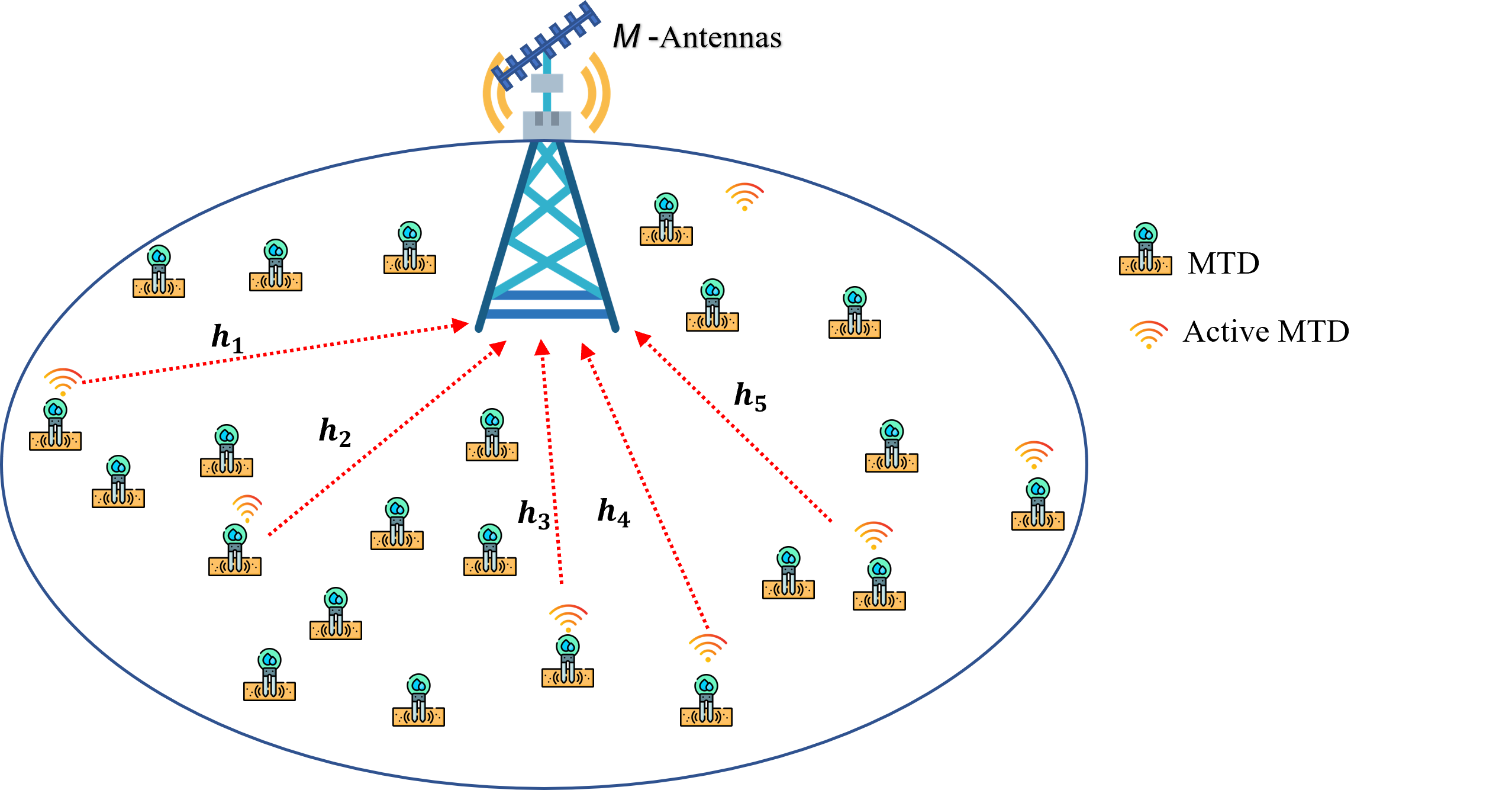
Figure 1: A massive machine-type communications network scenario, where $N$ MTDs transmit in the uplink to a BS equipped with $M$ antennas.

We consider a communication network scenario depicted by Figure 1, where a BS equipped with $M$ antennas serves a set of $N$ MTDs that transmit data in the uplink. To align with practical MTC, we assume that in a given coherence interval of $T$ symbols, an unknown set $\mathcal{K}\subset[\![N]\!]$ of cardinality $K=|\mathcal{K}|$ is active. Note that from these $T$ symbols of the coherence interval, $L$ symbols are used for metadata processing to identify the $K$ active MTDs. Meanwhile, the remaining $T-L$ symbols are used to transmit their payload data. Furthermore, we assume that each $n^{\text{th}}$ MTD is connected to the BS through a quasi-static fading uplink channel $\bm{h}_{n}\in\mathbb{C}^{M\times 1}$. For simplicity, we assume an independent Rayleigh small-scale fading model so that the channel vectors are statistically independent of each other and spatially white, i.e., $\bm{h}_{n}\sim\mathcal{CN}_{\!M}(\bm{0},\bm{I})$.

To account for the random activation of the MTDs, we define the activity indicator function as

$$\alpha_{n}\!=\!\begin{cases}1,\leavevmode\nobreak\ \text{if device $n$ is active}\\ 0,\leavevmode\nobreak\ \text{otherwise}\\ \end{cases}.$$ (1)

As a result of (1), $\alpha_{n}$ induces an effective channel $\bm{x}_{n}=\sqrt{\gamma_{n}}\bm{h}_{n}$ for the $n^{\text{th}}$ MTD. Here, $\gamma_{n}=\alpha_{n}\rho_{n}\beta_{n}$ is the effective power of the channel of the $n$-th MTD, where $\beta_{n}>0$ is the large-scale fading component (LSFC) of the $n^{\text{th}}$ device due to path-loss and shadowing, while $\rho_{n}$ is the device’s uplink transmission power. Hence, the concatenation of all the effective power levels of the channels of the MTDs in the network is defined by $\bm{\gamma}=(\gamma_{1},\ldots,\gamma_{N})^{\top}\in\mathbb{R}^{N}$. Similarly, let $\bm{X}=(\bm{x}_{1}\,\cdots\,\bm{x}_{N})^{\mbox{\scriptsize T}}\in\mathbb{C}^{N\times M}$ denote the concatenation of all the effective channel vectors. Since only a small set of MTDs are active, $\bm{X}$ is row-sparse. This leads to the uplink signal being a “compressively sensed” signal coming exclusively from active devices, as will be seen later. As such, the number of active MTDs is equivalent to the row-support of $\bm{X}\in\mathbb{C}^{N\times M}$. The index set of rows containing the non-zero elements is defined as

$$\mathcal{K} =\mathrm{supp}(\bm{X})\triangleq\{i\in[\![N]\!]:x_{nm}\neq 0\,\mbox{ for some $m\in[\![M]\!]$}\},$$

thus collecting the indices of the active devices, i.e., $\mathcal{K}=\{n\in[\![N]\!]:\alpha_{n}=1\}$. Note that due to the low likelihood of the MTDs being active simultaneously, $\lvert\mathcal{K}\rvert<N$ is a practical network property exploited in the CS-MUD framework, as will be shown next.

As mentioned earlier, $L$ symbols are used as pilot sequences, i.e., used mainly for metadata processing, such as to estimate the active MTDs. To avoid signaling overheads, these pilot sequences are normally preallocated by the BS and stored in the local memory of the MTDs. Let ${\bm{a}}_{n}\in\mathbb{C}^{L\times 1}$ denote the normalized pilot sequence of the $n^{\text{th}}$ MTD. These can be collected into a matrix $\bm{A}=({\bm{a}}_{1}\,\cdots\,{\bm{a}}_{N})\in\mathbb{C}^{L\times N}$. In the end, the first $L$ symbols of the noisy signal received at the BS, exclusively coming from the $K$ active MTDs, can now be modeled as

$$\bm{Y} =\sum_{k\in\mathcal{K}}\sqrt{\rho_{k}\beta_{k}}\alpha_{k}\bm{a}_{k}\bm{h}_{k}^{\mbox{\scriptsize T}}+\bm{W}$$

$$=\bm{A}\bm{X}+\bm{W},$$ (2)

where $\bm{W}\in\mathbb{C}^{L\times M}$ is an additive noise matrix whose elements are independent and identically distributed (i.i.d.) Gaussian random variables with known variance $\sigma^{2}>0$, i.e., $w_{lm}\sim\mathcal{CN}(0,\sigma^{2})$. Owing to the massiveness of the MTDs, the length of the pilot sequences is normally very short compared to the number of devices, i.e., $L\ll N$, essentially leading to non-orthogonal pilot sequences that can have noticeable mutual coherence [3, 4]. Therefore, the task of the BS is to identify the active users by estimating the row-support $\mathcal{K}$ of $\bm{X}$. However, the condition $L\ll N$ indicates (2) to follow an underdetermined system of equations, thus leading to an infinite number of solutions. To overcome this challenge, one needs to resort to CS-MUD methodology, such as those that were mentioned under Section I-A. In the sequel, we propose greedy pursuit approach for solving the Gaussian log-likelihood function, as we discuss next.

Since there is no correlation in the receive antennas, the columns $\{\bm{y}_{m}\in\mathbb{C}^{L}\}_{m=1}^{M}$ of $\bm{Y}$ are independent of each other. This means that $\bm{y}_{m}\sim\mathcal{CN}_{L}(\bm{0},\bm{\Sigma})$ has a positive definite Hermitian (PDH) $L\times L$ covariance matrix

$$\bm{\Sigma} =\bm{A}\bm{\Gamma}\bm{A}^{\mathsf{H}}+\sigma^{2}\bm{I}$$

$$=\sum_{n=1}^{N}\gamma_{n}{\bm{a}}_{n}{\bm{a}}_{n}^{\mathsf{H}}+\sigma^{2}\bm{I},$$ (3)

where $\bm{\Gamma}=\operatorname{diag}(\bm{\gamma})$ is a diagonal matrix containing the effective powers of the MTDs. Note that $\mathcal{K}=\mathrm{supp}(\bm{X})=\mathsf{supp}(\bm{\gamma})$, which makes it possible to estimate the support using (II). As such, covariance learning (CL-) based support recovery algorithms can be constructed by minimizing the negative log-likelihood function (LLF) of the data $\bm{Y}$. The negative LLF is defined by (after scaling by $1/M$ and ignoring additive constants)

$$\ell(\bm{\gamma})=\operatorname{tr}((\bm{A}\bm{\Gamma}\bm{A}^{\mathsf{H}}+\sigma^{2}\bm{I})^{-1}\hat{\bm{\Sigma}})+\log|\bm{A}\bm{\Gamma}\bm{A}^{\mathsf{H}}+\sigma^{2}\bm{I}|,$$ (4)

where $\hat{\bm{\Sigma}}$ is the sample covariance matrix (SCM),

$$\hat{\bm{\Sigma}}=\frac{1}{M}\sum_{m=1}^{M}\bm{y}_{m}\bm{y}_{m}^{\mathsf{H}}={M}^{-1}\bm{Y}\bm{Y}^{\mathsf{H}},$$

while $\operatorname{tr}(\cdot)$ and $|\cdot|$ denote the matrix trace and determinant, respectively. Based on the LLF in (4), we next construct a covariance-based greedy matching algorithm that estimates $\mathcal{K}$ by solving for $\bm{\gamma}$.

III Covariance based matching pursuit

Consider the conditional likelihood of (4) where device powers $\gamma_{n}$ for $n\neq i$ are known, and define

$$\bm{\Sigma}_{\backslash i}=\sum_{n\neq i}\gamma_{n}{\bm{a}}_{n}{\bm{a}}_{n}^{\mathsf{H}}+\sigma^{2}\bm{I}=\bm{\Sigma}-\gamma_{i}{\bm{a}}_{i}{\bm{a}}_{i}^{\mathsf{H}}$$ (5)

as the covariance matrix of $\bm{y}_{m}$-s when the contribution from the $i^{\text{th}}$ device is removed. As $\gamma_{n}$ for $n\neq i$ are assumed to be given, $\bm{\Sigma}_{\backslash i}$ is a known fixed matrix. It then follows that the conditional negative LLF for the single unknown $i^{\text{th}}$ device power is defined as

$$\ell_{i}(\gamma) =\operatorname{tr}((\bm{\Sigma}_{\setminus i}+\gamma{\bm{a}}_{i}{\bm{a}}_{i}^{\mathsf{H}})^{-1}\hat{\bm{\Sigma}})+\log|\bm{\Sigma}_{\setminus i}+\gamma{\bm{a}}_{i}{\bm{a}}_{i}^{\mathsf{H}}|.$$ (6)

This function has a unique optimal value that is given by [32]:

$$\gamma_{i}=\max\left(\frac{{\bm{a}}_{i}^{\mathsf{H}}\bm{\Sigma}_{\setminus i}^{-1}\hat{\bm{\Sigma}}\bm{\Sigma}_{\setminus i}^{-1}{\bm{a}}_{i}-{\bm{a}}_{i}^{\mathsf{H}}\bm{\Sigma}_{\setminus i}^{-1}{\bm{a}}_{i}}{({\bm{a}}_{i}^{\mathsf{H}}\bm{\Sigma}_{\setminus i}^{-1}{\bm{a}}_{i})^{2}},0\right),$$ (7)

where $\bm{\Sigma}_{\setminus i}$ is already defined in (5).

This result will be the foundation for developing the CL-MP algorithm. We follow the generic matching pursuit strategy (see, e.g., [33]), and our proposed CL-based method is an adaptation of the CL orthogonal matching pursuit (CL-OMP) algorithm developed in [34]. There are two important distinctions to [34]. First, we assume that the noise power level $\sigma^{2}$ is known as is common in mMTC applications. Second, unlike in [34], we follow the MP strategy instead of the OMP as in [34]. This allows us to skip the “update provisional solution” step of the OMP algorithm and to use the computationally light update rule for the inverse of the covariance matrix, thus, speeding up the computations. We denote the $k^{\text{th}}$ update of $\bm{\gamma}$ and $\mathcal{K}$ by $\bm{\gamma}^{(k)}$ and $\mathcal{K}^{(k)}$, respectively. Therefore, starting with $k=0$, our CL-MP algorithm follows the steps below.

Initialization phase. Set $k=0$, and $\bm{\gamma}^{(0)}=\bm{0}_{N\times 1}$, and $\mathcal{K}^{(0)}=\mathsf{supp}(\bm{\gamma}^{(0)})=\emptyset$ as initial solutions of device powers and the signal support, respectively. Then $(\bm{\Sigma}^{(0)})^{-1}=(1/\sigma^{2})\bm{I}$ is the initial inverse covariance matrix at the start of iterations.

Main Iteration phase consists of the following steps:

1) Sweep: Compute the errors

$$\epsilon_{i} =\min_{\gamma\geq 0}\ell_{i}(\gamma)$$ (8)

for each $i\in\mathcal{K}^{\complement}=[\![N]\!]\setminus\mathcal{K}^{(k)}$ using its unique optimal value

$$\gamma_{i}=\max\Big{(}\frac{{\bm{a}}_{i}^{\mathsf{H}}(\bm{\Sigma}^{(k)})^{-1}\hat{\bm{\Sigma}}(\bm{\Sigma}^{(k)})^{-1}{\bm{a}}_{i}-{\bm{a}}_{i}^{\mathsf{H}}(\bm{\Sigma}^{(k)})^{-1}{\bm{a}}_{i}}{({\bm{a}}_{i}^{\mathsf{H}}(\bm{\Sigma}^{(k)})^{-1}{\bm{a}}_{i})^{2}},0\Big{)}.$$

2) Update support: Find a minimizer, $i_{k}$ of $\epsilon_{i}$: $\forall i\in\mathcal{K}^{\complement}$, $\epsilon_{i_{k}}\leq\epsilon_{i}$, and update the support $\mathcal{K}^{(k+1)}=\mathcal{K}^{(k)}\cup\{i_{k}\}$.

3) Update the inverse covariance matrix: Since the new covariance matrix after support update is

$$\bm{\Sigma}^{(k+1)}=\bm{\Sigma}^{(k)}+\gamma_{i_{k}}{\bm{a}}_{i_{k}}{\bm{a}}_{i_{k}}^{\mathsf{H}},$$

its inverse covariance matrix $(\bm{\Sigma}^{(k+1)})^{-1}$ can be obtained using Sherman-Morrison formula as shown in line 5 of algorithm 1.

4) Stopping rule: If stopping rule is not met, then increment $k$ by 1 and repeat steps 1)-3). Several stopping rules can be used. For example, one can stop iterations after the fixed number (say $K_{\max}$) or when the added index has power level $\gamma_{i_{k}}$ that falls below some threshold level. In the former case, $K_{\max}$ serves as the maximum number of active devices expected to be active.

The error term $\epsilon_{i}$ in (8) has the following closed-form expression:

$$\epsilon_{i}=c+\log(1+\gamma_{i}{\bm{a}}_{i}^{\mathsf{H}}\bm{\Sigma}^{-1}{\bm{a}}_{i})-\gamma_{i}\frac{{\bm{a}}_{i}^{\mathsf{H}}\bm{\Sigma}^{-1}\hat{\bm{\Sigma}}\bm{\Sigma}^{-1}{\bm{a}}_{i}}{1+\gamma_{i}{\bm{a}}_{i}^{\mathsf{H}}\bm{\Sigma}^{-1}{\bm{a}}_{i}},$$ (9)

where we have for simplicity of notation written $\bm{\Sigma}=\bm{\Sigma}^{(k)}$ and where $c$ denotes an irrelevant constant that is not dependent on $\gamma_{i}$. Thus, w.lo.g., we set $c=0$. Then using that $\gamma_{i}$ is given by (7) we can write

$$1+\gamma_{i}{\bm{a}}_{i}^{\mathsf{H}}\bm{\Sigma}^{-1}{\bm{a}}_{i} =1+\frac{{\bm{a}}_{i}^{\mathsf{H}}\bm{\Sigma}^{-1}\hat{\bm{\Sigma}}\bm{\Sigma}^{-1}{\bm{a}}_{i}-{\bm{a}}_{i}^{\mathsf{H}}\bm{\Sigma}^{-1}{\bm{a}}_{i}}{({\bm{a}}_{i}^{\mathsf{H}}\bm{\Sigma}^{-1}{\bm{a}}_{i})^{2}}{\bm{a}}_{i}^{\mathsf{H}}\bm{\Sigma}^{-1}{\bm{a}}_{i}$$

$$=1+\frac{{\bm{a}}_{i}^{\mathsf{H}}\bm{\Sigma}^{-1}\hat{\bm{\Sigma}}\bm{\Sigma}^{-1}{\bm{a}}_{i}-{\bm{a}}_{i}^{\mathsf{H}}\bm{\Sigma}^{-1}{\bm{a}}_{i}}{{\bm{a}}_{i}^{\mathsf{H}}\bm{\Sigma}^{-1}{\bm{a}}_{i}}$$

$$=\frac{{\bm{a}}_{i}^{\mathsf{H}}\bm{\Sigma}^{-1}\hat{\bm{\Sigma}}\bm{\Sigma}^{-1}{\bm{a}}_{i}}{{\bm{a}}_{i}^{\mathsf{H}}\bm{\Sigma}^{-1}{\bm{a}}_{i}}\mbox{ when $\gamma_{i}>0$}.$$

Substituting this into the denominator of the last term in (9), we obtain

$$\epsilon_{i}=\log(1+\gamma_{i}{\bm{a}}_{i}^{\mathsf{H}}\bm{\Sigma}^{-1}{\bm{a}}_{i})-\gamma_{i}{\bm{a}}_{i}^{\mathsf{H}}\bm{\Sigma}^{-1}{\bm{a}}_{i}.$$ (10)

If $\gamma_{i}=0$, then $\epsilon_{i}=0$. This explains line 3 in algorithm 1.

Input :  $\hat{\bm{\Sigma}}=M^{-1}\bm{Y}\bm{Y}^{\mathsf{H}}$, $\bm{A}$, $\sigma^{2}$

Initialize :  $\bm{\Sigma}^{-1}=(1/\sigma^{2})\bm{I}$, $\mathcal{K}=\emptyset$

1

2for $k=1,\ldots,N$ do

3     

4     $\gamma_{i}\leftarrow\max\Big{(}\frac{{\bm{a}}_{i}^{\mathsf{H}}\bm{\Sigma}^{-1}\hat{\bm{\Sigma}}\bm{\Sigma}^{-1}{\bm{a}}_{i}-{\bm{a}}_{i}^{\mathsf{H}}\bm{\Sigma}^{-1}{\bm{a}}_{i}}{({\bm{a}}_{i}^{\mathsf{H}}\bm{\Sigma}^{-1}{\bm{a}}_{i})^{2}},0\Big{)}$, $\forall i\in\mathcal{K}^{\complement}$

5     $\epsilon_{i}\leftarrow\log(1+\gamma_{i}{\bm{a}}_{i}^{\mathsf{H}}\bm{\Sigma}^{-1}{\bm{a}}_{i})-\gamma_{i}{\bm{a}}_{i}^{\mathsf{H}}\bm{\Sigma}^{-1}{\bm{a}}_{i}$, $\forall i\in\mathcal{K}^{\complement}$

6     $\mathcal{K}\leftarrow\mathcal{K}\cup\{i_{k}\}$ with $i_{k}\leftarrow\arg\min_{i\in\mathcal{K}^{\complement}}\epsilon_{i}$

7     $\bm{\Sigma}^{-1}\leftarrow\bm{\Sigma}^{-1}-\dfrac{\gamma_{i_{k}}\bm{\Sigma}^{-1}{\bm{a}}_{i_{k}}{\bm{a}}_{i_{k}}^{\mathsf{H}}\bm{\Sigma}^{-1}}{1+\gamma_{i_{k}}{\bm{a}}_{i_{k}}^{\mathsf{H}}\bm{\Sigma}^{-1}{\bm{a}}_{i_{k}}}$

8     if stopping rule is met (see text) then

          break

      end if

     

end for

Output : A set $\mathcal{K}$, containing $I$ indices, where $I$ is the number of iterations completed.

Algorithm 1 Covariance Learning Matching Pursuit (CL-MP) algorithm

III-A Computational complexity comparisons

In Table I, we present the computational complexity analysis of CL-MP and some benchmark algorithms. In the complexity calculations, it is assumed that the number of antennas ($M$) is smaller than the number of users ($N$) and the pilot length ($L$) is smaller than $N$, which are typical scenarios in mMTC. In SOMP, the index $k$ denotes the iteration index (i.e., the number of atoms selected). The dominant complexity of CL-MP Algorithm 1 is the matrix-vector multiplications in lines 2, 3, and 5, whose complexity is $\mathcal{O}(L^{2})$. In lines 2 and 3, one performs computations for (essentially) all $N$ devices and hence the total complexity of these steps is $\mathcal{O}(NL^{2})$. In line 3, one searches the smallest value in a set of $N$ scalars with linear complexity $\mathcal{O}(N)$. In line 5, the inverse $\bm{\Sigma}^{-1}$ is computed using a rank-one update, which further improves the computational efficiency as inverting an $L\times L$ matrix is not needed (which is of complexity $\mathcal{O}(L^{3})$ instead of $\mathcal{O}(L^{2})$. Hence, the full complexity of Algorithm 1 per iteration is $\mathcal{O}(NL^{2})$. Thus the complexity of CL-MP is linear in $N$ and quadratic in $L$. This is a desired feature for low-latency mMTC scenarios where the number of MTDs $N$ is large while the pilot length $L$ is often small. Note that SBL and VAMP grow quadratic in $N$.

It can also be noted that the computational complexity of CL-MP is the same as that of CWO per iteration. However, CL-MP is a greedy approach, while CWO is iterative, whose best performance is obtained after the algorithm’s convergence. Unlike iterative approaches, greedy methods do not suffer from convergence issues, which often happens when the nominal assumptions do not hold (e.g., when Gaussianity of data does not hold or in the presence of outliers).

It should also be stressed that the final complexity of all algorithms is the complexity per iteration times the number of iterations $I$ needed for convergence. For example, for SBL the full complexity is $\mathcal{O}(IN^{2}L)$. It is well known that the Expectation Maximization (EM) algorithm utilized by SBL suffers from slow convergence, and thus $I$ can often be very large. Such problems are not faced by greedy pursuit approaches which aim to find the minimum of the LLF greedily instead of using an iterative optimization algorithm.

Table I: Computational complexity of CS-MUD algorithms.

Algorithm	Complexity (per iteration)
CL-MP	$\mathcal{O}(NL^{2})$
CWO [28]	$\mathcal{O}(NL^{2})$
VAMP [35]	$\mathcal{O}(N^{2}M)$
SBL [36]	$\mathcal{O}(N^{2}L)$
SOMP [37]	$O(L\cdot\max(NM,k^{2})+k^{3})$

IV Empirical comparisons

This section validates the performance of the proposed CL-MP algorithm under a variety of settings. As performance metrics, we used missed detection and exact recovery. Missed detection (MD) occurs when a device is active but detected inactive. Therefore, the (empirical) probability of misdetection is the Monte Carlo (MC) average ratio of the number of such devices relative to the total number of active MTDs and is defined as

$$\text{P}_{md}=\frac{1}{Q}\sum_{q=1}^{Q}\frac{|\mathcal{K}\setminus\mathcal{K}^{(q)}|}{|\mathcal{K}|},$$ (11)

where $Q$ is the number of MC trials, and $\mathcal{K}^{(q)}$ is the estimate of the support $\mathcal{K}$ of the $q^{\text{th}}$ MC trial. On the other hand, exact recovery (ER) of devices occurs when active devices are correctly detected, and it is defined by

$$\text{P}_{er}=\frac{1}{Q}\sum_{q=1}^{Q}\mathbbm{1}(\mathcal{K}^{(q)}=\mathcal{K}).$$ (12)

We note that the indices of active devices $\mathcal{K}$ (with $|\mathcal{K}|=K$) for each $q^{\text{th}}$ MC trial are also randomly selected from set $[\![N]\!]$ without replacement.

IV-A The effect of $M$, $L$ and $K$

 

Figure 2: Probability of misdetection (top) and exact recovery (bottom) vs $M$ for different levels of active devices ($K$); $L=64$, $N=1000$, and LSFC-s $\beta_{n}\sim Unif(-15,0)$ on dB scale.

We first investigate the effects of $L$, $M$, and $K$ on the AUD performance. We let the LSFCs $\beta_{n}$, $\forall n$ to follow uniform distribution in dB scale, i.e., $10\log_{10}(\beta_{n})$ is uniformly distributed in range $[10\log_{10}(\beta_{\text{min}}),10\log_{10}(\beta_{\text{max}})]$. We compare the proposed CL-MP in algorithm 1 against the CWO algorithm [28, Algorithm 1]. We set the maximum number of iterations of the CWO algorithm to 15. To make the comparisons fair, we assume that the number of active devices $K$ is known to both algorithms. Hence the CL-MP algorithm is terminated after $K$ iterations and directly returns the estimated support $\hat{\mathcal{K}}$ of size $|\hat{\mathcal{K}}|=K$. In the case of the CWO algorithm, thresholding is needed. Here, the active users are identified by picking the positions of the $K$ largest entries of the final estimate $\hat{\bm{\gamma}}$. The number of MC runs is $2000$.

Figure 3: Top:Average running time in seconds for different $K$ when $L=64$ and $N=1000$. Bottom: Average running time for different $L$ and $K$ when $M=40$ for CWO (left panel) and CL-MP (right panel) methods.

Figure 2 displays the probability of misdetection and exact recovery as a function of number of antennas ($M$) and for different numbers of active devices ($K$). Bernoulli pilot sequence of length $L=64$ are used and the number of devices is $N=1000$. The pilots are normalized to unit energy per symbol, i.e., $\|{\bm{a}}_{n}\|_{2}^{2}=L$. LSFC coefficients follow a uniform distribution with a range $[-15,0]$ dB. Both methods show similar performance, but the CL-MP has a slight advantage in all levels of $K$ and $M$. In addition to this, the running times (on MacBook Pro laptop 2.3GH Intel i9) are shown in the top panel of Figure 3 demonstrate that it achieves high-level performance in significantly lower running time than the CWO algorithm. The differences between the methods are more pronounced when the number of active devices is small. Since CWO and CL-MP algorithms do not scale with $M$, the CPU bars are averages over all instances of $M$.

Figure 4 displays the probability of misdetection and exact recovery as a function of pilot sequence length ($L$) and for different levels of active devices ($K$) when the number of antennas is fixed ($M=40$). Again, we can note that the proposed CL-MP performed better for all levels of $K$ and $L$. The running times (on MacBook Pro laptop 2.3GH Intel i9) for both methods are displayed at the bottom panel of Figure 3. As noted, CL-MP scales better with $L$ than CWO, and the advantage is, as expected, more significant when $K$ is small.

 

Figure 4: Probability of misdetection (top) and exact recovery (bottom) vs $L$ for different levels of active devices ($K$); $N=1000$, $M=40$ and LSFC-s $\beta_{n}\sim Unif(-15,0)$ on dB scale.

IV-B MIMO uplink network simulation

In this subsection, we present the results of the performance of our proposed CL-MP in the mMTC network. For these simulations, we consider a single-cell massive MIMO uplink network, where a BS serves $1000$ MTDs randomly placed within the cell between a radius of $25$ m and $250$ m. We adopt a log-distance path loss model where LSFC is $\beta_{n}=-130-37.6\log_{10}d_{n}$, where $d_{n}$ is the distance between the $n^{\text{th}}$ MTD and the BS. For resource fairness, we assume uplink power control following channel inversion, such that each MTD transmits with power[8]

$$\rho_{n}=\frac{p^{\mathrm{max}}\beta_{\mathrm{min}}}{\beta_{n}},$$ (13)

where $\beta_{\mathrm{min}}$ is the large-scale effect at the edge of the cell and $p^{\mathrm{max}}$ is the maximum allowable power for each MTD. Consequently, the received signal-to-noise ratio (SNR) for each MTD is defined by

$$\text{SNR}_{n}=\frac{p^{\mathrm{max}}\beta_{\mathrm{min}}}{\sigma^{2}}.$$ (14)

Unless otherwise stated, the simulation parameters used in this paper are summarized in Table II.

For the performance benchmark, we compare CL-MP with Vector AMP (VAMP) [35], SBL [36], and SOMP [37]. We acknowledge that all these benchmark solutions first estimate $\bm{X}$, then map it to $\hat{\bm{\alpha}}$. To ensure fairness in our comparison, we input the number of active MTDs $K$ into each algorithm. This ensures that $K$ indices corresponding to maximum row norms are selected from matrix $\bm{X}$ after the convergence of each algorithm. Therefore, the set of indices of the selected $K$ rows will serve as an estimate $\hat{\mathcal{K}}$ of $\mathcal{K}$ at the end of each algorithm. Each algorithm will have two stopping criteria, i.e. if the maximum number of iterations $T_{max}$ has been reached or the relative change between two consecutive estimates $\Delta$ becomes insignificant. For random sensing matrices, we use the Gaussian pilot sequences, which we denote by G-MAT, and the Bernoulli pilot sequences, which we denote by B-MAT. For structured pilot sequences, we generate pilot sequences following the restrictively combined fixed orthogonal block matrix from [4], which we denoted by RC-FOBM as well as restively combined random orthogonal block matrix, which we denote by RC-ROBM.

Table II: Simulation parameters

Parameter	Value
Cell radius	$250$ m
Number of MTDs $(N)$	$1000$
Bandwidth	$20$ MHz
Noise power ($\sigma^{2}$)	$2\!\times\!10^{-13}$ W
Coherence interval $(T)$	$300$
Length of the pilot sequences $(L)$	$64$
Number of BS antennas $(M)$	$32$
Activation probability $(\epsilon)$	$0.01$
$\text{Maximum MTD power}(p^{\text{max}})$	$0.1$ W
Average SNR	$10$ dB
Error tolerance $(\Delta)$	$10^{-6}$
Monte Carlo $(\text{MC})$	$2000$
Maximum Iterations $(T_{max})$	$150$

Fig. 5 presents the results in terms of the $\text{P}_{md}$ as a function of the SNR, for different algorithms. The general trend shows that increasing SNR improves the $\text{P}_{md}$ of all the algorithms. This is because as the SNR increases, the desired signal component, which in our case is represented by $\bm{A}\bm{X}$, has higher power relative to the noise. As a result, it becomes easier to recover and identify the active users. The results show that both SBL and CL-MP have comparable performance as the SNR increases and their performance is superior to that of the SOMP and VAMP. The comparable performance between SBL and CL-MP is due to the equivalence of their objective functions as mentioned in Section I-B. However, the superior performance of CL-MP validates the proposed solutions. Since CL-MP has a similar performance as SBL, we next evaluate its performance for different sensing matrices.

Figure 5: $\text{P}_{md}$ as a function of SNR for different algorithms

Figure 6: $\text{P}_{md}$ of CL-MP as a function of the SNR.

Fig. 6 presents the performance in terms of the probability of miss detection ($\text{P}_{md}$) as a function of the SNR and the structure of the pilot sequences used. Similar to the results in Fig. 5, the performance generally improves as the SNR increases. Despite this, the proposed solution CL-MP performs differently for varying sensing matrices. This shows the non-triviality of choosing pilot sequences in MTC [4, 3]. For instance, the performance is superior when using Bernoulli pilot sequences and least when using the Gaussian pilot sequences. This is because pilot sequences such as Gaussian tend to increase the collision probability of the pilot sequences, thus, degrading the performance [4, 3, 8]. On the other hand, Bernoulli, RC-FOBM, and RC-ROBM have reduced collision probabilities and thus have better performance than the Gaussian pilot sequences. Despite this, the proposed CL-MP performs reasonably well under the different set of pilot sequences. Another interesting result is that the CL-MP performs reasonably well at very low SNR values, reaching $P_{md}=0.01$ for BMAT at SNR of $0$ dB.

Figure 7: $\text{P}_{md}$ as a function of the number of antennas

Fig. 7 shows the performance in terms of $\text{P}_{md}$ as a function of the number of antennas for different algorithms. The general trend shows that the performance of all the algorithms improves with an increase in the number of antennas ($M$). This is mainly because an increase in $M$ imposes more structural sparsity on the matrix $\bm{X}$, thus increasing the accuracy of the estimation. This reveals the advantage of having multiple BS antennas, which leads to a multiple measurement vector (MMV) problem in compressed sensing[8]. However, it can be observed that both CL-MP and SBL have equivalent and superior performance compared to VAMP and SOMP, thus, confirming the superiority of our proposed solution. Though both SBL and CL-MP are comparable in terms of performance in $\text{P}_{md}$, it is worth emphasizing that CL-MP has lower computational complexity than SBL, as shown in Table I, making it a more practical solution in MTC. To substantiate this, we compare the run-times for varying $M$.

Figure 8: Run-time as a function of the number of antennas

Figure 8 presents the results of the run-times of each algorithm for a different number of antennas of the BS. Effectively, this reveals how each algorithm scales up. From the results, it can be observed that the proposed CL-MP has superior scale-up properties as compared to all the benchmarks. On the other hand, it is worth noting that, even though SBL has similar performance as the CL-MP in terms of $\text{P}_{md}$, it takes a longer time to run and is thus not favorable in mMTC.

Figure 9: $\text{P}_{md}$ as a function of the pilot lengths for different algorithms.

Fig. 9 shows the performance as a function of the pilot lengths ($L$) for different algorithms. The trend reveals that the $\text{P}_{md}$ reduces as the pilot length increases. This is mainly due to better pilot structure as the length increases. Essentially, the signal detection phase is done over a longer period, thus improving the accuracy of the channel estimation for SOMP, VAMP and SBL, as well as the index estimation of the CL-MP. Similar to the results in Fig 7 and Fig. 5, CL-MP and SBL perform better than all the other benchmarks. Consistent with the results of Fig. 8, CL-MP has the added advantage of being more scalable.

Figure 10: Runtime of CL-MP as a function of the number $N$ of the MTDs in the network

To conclude the results, Fig. 10 presents the runtime of CL-MP as a function of the number of MTDs. In general, the runtime increases with the number of MTDs, which is expected because the size of $\bm{\gamma}$ increases. Despite this, the CL-MP has lower runtimes for a large number of users. For instance, it takes approximately $1$ second for CL-MP to recover and perform AUD from the signal received from $N=6000$ users when the pilot length is $L=72$. This translates to better runtime than SBL, which is shown to require more than $5$ seconds to process signals from $N=1000$ users in Fig. 8. To further support the results of Fig. 10, in Fig. 11, we present the results of $\text{P}_{md}$ for varying sizes of the networks. In general, the proposed CL-MP algorithm is effective in solving AUD problems, with very low $\text{P}_{md}$ even in very large MTC networks, rendering our proposal a practical solution for the rapidly growing MTC networks.

Figure 11: $\text{P}_{md}$ as a function of the number $N$ of the MTDs in the network.

V Conclusions and Future Directions

This paper introduces a novel framework for estimating the active user indices in MTC. The proposed technique uses the covariance of the received signal to formulate an optimization problem for the sparse effective power levels in MTC and solves it using a greedy approach. The results demonstrate that the proposed framework offers highly accurate device activity detection with very low runtimes. However, while efficient, the proposed solution does not estimate the activation probability. Therefore, the results of this work can be extended to incorporate activation probability estimation as future research direction. Moreover, considering that the IoT framework will eventually be served by Low Earth Orbit (LEO) satellites, one potential extension of this work could be the integration of CL-MP in satellite receivers, where the channel has a line of sight.

References

- [1] H. Shariatmadari, R. Ratasuk, S. Iraji, A. Laya, T. Taleb, R. Jäntti, and A. Ghosh, “Machine-type communications: Current status and future perspectives toward 5G systems,” IEEE Communications Magazine, vol. 53, no. 9, pp. 10–17, 2015.
- [2] E. Dutkiewicz, X. Costa-Perez, I. Z. Kovacs, and M. Mueck, “Massive machine-type communications,” IEEE Network, vol. 31, no. 6, pp. 6–7, 2017.
- [3] L. Marata, O. L. A. López, H. Djelouat, M. Leinonen, H. Alves, and M. Juntti, “Joint coherent and non-coherent detection and decoding techniques for heterogeneous networks,” IEEE Transactions on Wireless Communications, vol. 22, no. 3, pp. 1730–1744, 2022.
- [4] L. Marata, O. L. A. López, A. Hauptmann, H. Djelouat, and H. Alves, “Joint activity detection and channel estimation for clustered massive machine type communications,” IEEE Transactions on Wireless Communications, pp. 1–1, 2023.
- [5] J. Gao, Y. Wu, T. Li, and W. Zhang, “Energy Efficiency of MIMO Massive Unsourced Random Access with Finite Blocklength,” IEEE Wireless Communications Letters, 2023.
- [6] Y. Liu, S. Zhang, X. Mu, Z. Ding, R. Schober, N. Al-Dhahir, E. Hossain, and X. Shen, “Evolution of NOMA toward next generation multiple access (NGMA) for 6G,” IEEE Journal on Selected Areas in Communications, vol. 40, no. 4, pp. 1037–1071, 2022.
- [7] J. Choi, J. Ding, N.-P. Le, and Z. Ding, “Grant-free random access in machine-type communication: Approaches and challenges,” IEEE Wireless Communications, vol. 29, no. 1, pp. 151–158, 2021.
- [8] K. Senel and E. G. Larsson, “Grant-free massive MTC-enabled massive MIMO: A compressive sensing approach,” IEEE Transactions on Communications, vol. 66, no. 12, pp. 6164–6175, 2018.
- [9] L. Liu, E. G. Larsson, W. Yu, P. Popovski, C. Stefanovic, and E. De Carvalho, “Sparse signal processing for grant-free massive connectivity: A future paradigm for random access protocols in the Internet of Things,” IEEE Signal Processing Magazine, vol. 35, no. 5, pp. 88–99, 2018.
- [10] B. Li, J. Zheng, and Y. Gao, “Compressed sensing based multiuser detection of grant-free NOMA with dynamic user activity,” IEEE Communications Letters, vol. 26, no. 1, pp. 143–147, 2021.
- [11] J. Liu, G. Wu, X. Zhang, S. Fang, and S. Li, “Modeling, analysis, and optimization of grant-free NOMA in massive MTC via stochastic geometry,” IEEE Internet of Things Journal, vol. 8, no. 6, pp. 4389–4402, 2020.
- [12] X. Zhang, P. Fan, J. Liu, and L. Hao, “Bayesian learning-based multiuser detection for grant-free NOMA systems,” IEEE Transactions on Wireless Communications, vol. 21, no. 8, pp. 6317–6328, 2022.
- [13] R. B. Di Renna, C. Bockelmann, R. C. de Lamare, and A. Dekorsy, “Detection techniques for massive machine-type communications: Challenges and solutions,” IEEE Access, vol. 8, pp. 180 928–180 954, 2020.
- [14] Y. Polyanskiy, “A perspective on massive random-access,” in IEEE International Symposium on Information Theory (ISIT). IEEE, 2017, pp. 2523–2527.
- [15] X. Shao, X. Chen, D. W. K. Ng, C. Zhong, and Z. Zhang, “Cooperative activity detection: Sourced and unsourced massive random access paradigms,” IEEE Transactions on Signal Processing, vol. 68, pp. 6578–6593, 2020.
- [16] A. E. Kalør, G. Duris, S. Coleri, S. Parkvall, W. Yu, A. Mueller, and P. Popovski, “Wireless 6G Connectivity for Massive Number of Devices and Critical Services,” arXiv preprint arXiv:2401.01127, 2024.
- [17] J. Ni and J. Zheng, “Non-coherent grant-free NOMA through pilot-and channel block-index modulation,” IEEE Wireless Communications Letters, vol. 10, no. 4, pp. 705–709, 2020.
- [18] O. L. López, N. H. Mahmood, M. Shehab, H. Alves, O. M. Rosabal, L. Marata, and M. Latva-Aho, “Statistical tools and methodologies for ultrareliable low-latency communication—a tutorial,” Proceedings of the IEEE, vol. 111, no. 11, pp. 1502–1543, 2023.
- [19] Z. Zhang, Q. Guo, Y. Li, M. Jin, and C. Huang, “Variational Bayesian inference clustering based joint user activity and data detection for grant-free random access in mMTC,” IEEE Internet of Things Journal, 2023.
- [20] X. Zhang, F. Labeau, L. Hao, and J. Liu, “Joint active user detection and channel estimation via Bayesian learning approaches in MTC communications,” IEEE Transactions on Vehicular Technology, vol. 70, no. 6, pp. 6222–6226, 2021.
- [21] J. Wang, J. Yi, R. Han, L. Bai, and J. Choi, “Variational Bayesian inference for channel estimation and user activity detection in C-RAN,” IEEE Wireless Communications Letters, vol. 9, no. 7, pp. 953–956, 2020.
- [22] H. Djelouat, M. Leinonen, L. Ribeiro, and M. Juntti, “Joint user identification and channel estimation via exploiting spatial channel covariance in mMTC,” IEEE Wireless Communications Letters, vol. 10, no. 4, pp. 887–891, 2021.
- [23] G. Sun, M. Cao, W. Wang, W. Xu, and C. Studer, “Joint active user detection, channel estimation, and data detection for massive grant-free transmission in cell-free systems,” in IEEE 24th International Workshop on Signal Processing Advances in Wireless Communications (SPAWC). IEEE, 2023, pp. 406–410.
- [24] L. Zhu, K.-H. Liu, L. Wan, and L. Sun, “Active user detection and channel estimation via fast ADMM,” in IEEE Wireless Communications and Networking Conference (WCNC). IEEE, 2023, pp. 1–6.
- [25] Z. Chen, F. Sohrabi, Y.-F. Liu, and W. Yu, “Covariance based joint activity and data detection for massive random access with massive MIMO,” in IEEE International Conference on Communications (ICC). IEEE, 2019, pp. 1–6.
- [26] Y.-F. Liu, W. Yu, Z. Wang, Z. Chen, and F. Sohrabi, “Grant-free random access via covariance-based approach,” Next Generation Multiple Access, pp. 391–414, 2024.
- [27] W. Liu, Y. Cui, F. Yang, L. Ding, and J. Sun, “MLE-based device activity detection under Rician fading for massive grant-free access with perfect and imperfect synchronization,” IEEE Transactions on Wireless Communications, 2024.
- [28] A. Fengler, S. Haghighatshoar, P. Jung, and G. Caire, “Non-Bayesian activity detection, large-scale fading coefficient estimation, and unsourced random access with a massive MIMO receiver,” IEEE Transactions on Information Theory, vol. 67, no. 5, pp. 2925–2951, 2021.
- [29] J. You, W. Wang, S. Liang, W. Han, and B. Bai, “An efficient two-stage SPARC decoder for massive MIMO unsourced random access,” IEEE Transactions on Wireless Communications, 2023.
- [30] N. Y. Yu and W. Yu, “Joint activity and data detection for massive grant-free access using deterministic non-orthogonal signatures,” IEEE Transactions on Wireless Communications, 2024.
- [31] L. Marata, “Advanced signal processing techniques for machine type communications,” 2024.
- [32] T. Yardibi, J. Li, P. Stoica, M. Xue, and A. B. Baggeroer, “Source localization and sensing: A nonparametric iterative adaptive approach based on weighted least squares,” IEEE Transactions on Aerospace and Electronic Systems, vol. 46, no. 1, pp. 425–443, 2010.
- [33] M. Elad, Sparse and redundant representations. New York: Springer, 2010.
- [34] E. Ollila, “Sparse signal recovery and source localization via covariance learning,” arXiv preprint arXiv:2401.13975, 2024.
- [35] L. Liu and W. Yu, “Massive connectivity with massive MIMO—Part I: Device activity detection and channel estimation,” IEEE Transactions on Signal Processing, vol. 66, no. 11, pp. 2933–2946, 2018.
- [36] D. P. Wipf and B. D. Rao, “Sparse bayesian learning for basis selection,” IEEE Transactions on Signal processing, vol. 52, no. 8, pp. 2153–2164, 2004.
- [37] J. A. Tropp, “Algorithms for simultaneous sparse approximation. Part II: Convex relaxation,” Signal Processing, vol. 86, no. 3, pp. 589–602, 2006.