Hypersurfaces with capillary boundary evolving by volume preserving power mean curvature flow

Carlo Sinestrari (Carlo Sinestrari) Dipartimento Di Matematica, Università degli Studi di Roma "Tor Vergata", Via della Ricerca Scientifica, 00133, Roma, Italy sinestra@mat.uniroma2.it  and  Liangjun Weng (Liangjun Weng) Dipartimento Di Matematica, Università degli Studi di Roma "Tor Vergata", Via della Ricerca Scientifica, 00133, Roma, Italy liangjun.weng@uniroma2.it
Abstract.

In this paper, we introduce a volume- or area-preserving curvature flow for hypersurfaces with capillary boundary in the half-space, with speed given by a positive power of the mean curvature with a non-local averaging term. We demonstrate that for any convex initial hypersurface with a capillary boundary, the flow exists for all time and smoothly converges to a spherical cap as $t\to+\infty$.

Key words and phrases:
Mean curvature flow, capillary isoperimetric ratio, pinching estimate, curvature estimates
2020 Mathematics Subject Classification:
Primary: 53E10. Secondary: 35B40, 35K93

1. Introduction

In this paper, we investigate the behavior of a curvature flow of capillary hypersurfaces with a prescribed contact angle condition at the boundary. Curvature flows have been widely investigated in the case of a closed manifold, starting from the classical paper of Huisken [27] on mean curvature flow, which is a time-dependent family of immersions $X:M^{n}\times[0,T)\to\mathbb{R}^{n+1}$ of an $n$-dimensional manifold satisfying

$\displaystyle\partial_{t}X=-H\nu,$

where $\nu$ is the outer normal and $H$ is the mean curvature. In [27] it was proved that the mean curvature flow collapses arbitrary initial convex hypersurface to round points in finite time, and this result was the starting point of a fruitful line of research on the formation of singularities which led to relevant geometric applications through the decades.

Later, Schulze [45, 46, 47] considered a flow of the form $\partial_{t}X=-H^{\alpha}\nu$ for a general power $\alpha>0$ of the mean curvature. He proved that convex hypersurfaces collapse to a point and that the asymptotic shape is round if $\alpha>1$ and if the principal curvatures of the initial surface are sufficiently pinched. The analysis of a general power has various motivations. As observed in [45], the $H^{\alpha}$-flow is the gradient flow of the area functional of $\Sigma_{t}:=X(M^{n},t)$ with respect to the $L^{\frac{\alpha+1}{\alpha}}$-norm, generalizing a well-known property in the $\alpha=1$ case. Furthermore, a weak formulation of the $H^{\alpha}$-flow was later used in [48] to prove isoperimetric inequalities in Riemannian manifolds. We further mention two very recent papers, where it is shown that the power mean curvature flow occurs respectively as the limit of the level set flow of a time-fractional Allen-Cahn equation [19] and of a suitable minimizing movement evolution of sets [10]. In addition to the powers of the mean curvature, a vast literature has been devoted to hypersurface flows where the speed is given by general nonlinear functions of the principal curvatures, see e.g. [2, 4, 7, 8, 13] and the references therein.

In [28], Huisken considered a a non-local variant of the mean curvature flow,

$\displaystyle\partial_{t}X=(h(t)-H)\nu,$ (1.1)

where $h(t):=\frac{1}{|\Sigma_{t}|}\int_{\Sigma_{t}}HdA$ is chosen to ensure that the volume enclosed by $\Sigma_{t}$ remains constant. A remarkable feature of this flow is that the area $|\Sigma_{t}|$ is monotone decreasing so that the isoperimetric ratio of the enclosed domain improves with the flow. Huisken proved that if $\Sigma_{0}$ is convex then the flow (1.1) has a solution for all times and converges smoothly to a round sphere as $t\to+\infty$. McCoy [35] obtained the same convergence result by modifying the term $h(t)$ in (1.1) in order to keep the area $|\Sigma_{t}|$ constant; in this case, the enclosed volume is increasing and the isoperimetric ratio is again improving. Similar results were then obtained for other constrained curvature flows in various settings [3, 14, 15, 36, 37, 38].

In [49], the first author studied the flow analogous to [28] for a general power $\alpha>0$ of the mean curvature,

$\displaystyle\partial_{t}X=(h(t)-H^{\alpha})\nu.$ (1.2)

The main observation was that the monotonicity properties of the constrained flows can be used as a tool to obtain better convergence results than in the standard case (similar ideas had already been used in [3, 14] in the case $\alpha=1$). In [49] it was proved that (1.2) drives any convex initial data to a round sphere as $t\to\infty$ for a general $\alpha>0$. We remark that, for the standard (local) power mean curvature flow, the smooth convergence to a round profile is only known under strong curvature pinching assumptions on the data if $\alpha>1$ [46], and it is even false for some values of $\alpha<1$, see the introduction in [49] for a more detailed discussion. Similar monotonicity-based techniques, coupled with powerful results of convex analysis, have been applied to more general classes of flows in recent years, see [6, 9, 11, 12]

In [22], Guan-Li invented a local type of mean curvature flow, which is also volume preserving and area decreasing as the non-local flow in [28]. Its speed function is given by $\partial_{t}X=(n-\langle X,\nu\rangle H)\nu$, and this flow drives star-shaped closed hypersurfaces to a round sphere as $t\to+\infty$. See also [16, 21, 23, 24], which give many other significant developments for similar flows in various settings afterward. In particular, we point out that the monotonicity properties of these flows, both in the local and nonlocal case, have been applied to obtain geometric inequalities of the Alexandrov-Fenchel type, possibly for more general domains than in the classical setting of convex analysis.

While all the above references deal with closed hypersurfaces, our interest in this paper lies in studying hypersurfaces with boundary satisfying a Neumann condition. This case has also been studied for a long time, see e.g. [50], but initially fewer results were known compared to the closed case. In recent years, research has made great strides in constructing flows for hypersurfaces with boundaries and obtaining geometric inequalities. For instance, works such as [43] and [55] have investigated the inverse nonlinear curvature flow for hypersurfaces with free and capillary boundaries in the Euclidean unit ball respectively, and have derived some new Alexandrov-Fenchel type inequalities. For capillary hypersurfaces in the half-space, references such as [39] and [26, 53, 54] have explored mean curvature flow and inverse curvature flow with capillary boundaries in the half-space, respectively. Very recently, the asymptotic behavior of capillary convex hypersurface evolving by the Gauss curvature type flow was analyzed in [40]. All these works on flows with boundary concern local type flows. In this paper, instead, we design and analyze a nonlocal flow corresponding to (1.2) for hypersurfaces with capillary boundaries in the half-space. To the best of our knowledge, non-local curvature flows with boundary in the smooth setting have only been studied in dimension $n=1$, such as the area-preserving curve shortening flow with free boundary in $\mathbb{R}^{2}$ analyzed by Mäder-Baumdicker [32, 33].

Typically, non-local type flows pose different challenges compared to their local counterparts. In particular, some maximum principle arguments can no longer be applied and well-known properties of the local case, such as the avoidance principle, do no longer hold. The capillary setting also poses additional difficulties because it requires analysis of the boundary behavior of geometric quantities. On the other hand, it is remarkable that, by suitably modifying the geometric quantities, we are able to recover in the capillary case the essential properties used for the convergence result in the closed case [49], in particular the monotonicity of the isoperimetric ratio adapted to the capillary setting.

To describe our results, we introduce some notation and definitions. Let $\Sigma$ be a compact hypersurface in the Euclidean closed half-space $\overline{\mathbb{R}^{n+1}_{+}}:=\{x\in\mathbb{R}^{n+1}\,|\,\langle x,E_{n+1}\rangle\geq 0\}$ ($n\geq 1$), with boundary $\partial\Sigma$ lying in $\partial\mathbb{R}^{n+1}_{+}$, where $E_{n+1}=(0,\ldots,0,1)$ is the unit inner normal to $\partial\mathbb{R}^{n+1}_{+}$ in $\overline{\mathbb{R}^{n+1}_{+}}$. Such a hypersurface is called a capillary hypersurface if $\Sigma$ intersects $\partial{{\mathbb{R}}}_{+}^{n+1}$ at a constant contact angle $\theta\in(0,\pi)$ along $\partial\Sigma$, that is,

$\displaystyle\langle\nu,E_{n+1}\rangle=\cos\theta,\leavevmode\nobreak\ \leavevmode\nobreak\ \leavevmode\nobreak\ \text{ on }\partial\Sigma,$ (1.3)

where $\nu$ is the unit outward normal of $\Sigma$. In particular, if $\Sigma$ meets the boundary orthogonally, i.e. $\theta=\frac{\pi}{2}$, it is called a hypersurface with free boundary. Denote $\widehat{\Sigma}$ the bounded domain in $\overline{\mathbb{R}^{n+1}_{+}}$ enclosed by $\Sigma\subset\overline{\mathbb{R}^{n+1}_{+}}$ and by $\partial\mathbb{R}^{n+1}_{+}$. The boundary of $\widehat{\Sigma}$ consists of two parts: one is $\Sigma$ and the other, which will be denoted by $\widehat{\partial\Sigma}$, lies on $\partial\mathbb{R}^{n+1}_{+}$. $\Sigma$ and $\widehat{\partial\Sigma}$ have a common boundary $\partial\Sigma$. The well-known capillary area functional (see for instance the comprehensive books by Finn [20, Section 1.4] and Maggi [34, Chapter 19]) for $\Sigma$ is defined as

$\displaystyle W_{\theta}(\widehat{\Sigma}):=|\Sigma|-\cos\theta|\widehat{\partial\Sigma}|.$

Moreover, it is easy to see that (see e.g. [41, Lemma 2.14] or [42, Remark 2.1])

$\displaystyle W_{\theta}(\widehat{\Sigma})=\int_{\Sigma}(1-\cos\theta\langle\nu,E_{n+1}\rangle)dA.$ (1.4)

Let $M$ be a $n$-dimensional smooth compact manifold with boundary $\partial M$ and $\Sigma_{0}:=X_{0}(M)\subset\overline{\mathbb{R}^{n+1}_{+}}$ be a capillary hypersurface with contact angle $\theta\in(0,\pi)$. We consider a family of smooth capillary hypersurfaces $\Sigma_{t}$ in $\overline{\mathbb{R}^{n+1}_{+}}$ starting from $\Sigma_{0}$, given by the embeddings $X:M\times[0,T)\to\overline{\mathbb{R}^{n+1}_{+}}$ and satisfying

$\displaystyle\left\{\begin{array}[]{llll}\partial_{t}X&=&(\phi(t)-H^{\alpha})\widetilde{\nu},&\hbox{ in }M\times[0,T),\\ \langle\nu,E_{n+1}\rangle&=&\cos\theta&\hbox{ on }\partial M\times[0,T),\\ X(\cdot,0)&=&X_{0}(\cdot)&\hbox{ on }M,\end{array}\right.$ (1.8)

where $\widetilde{\nu}:=\nu-\cos\theta E_{n+1}$ is the capillary outward normal of $\Sigma_{t}\subset\overline{\mathbb{R}^{n+1}_{+}}$. It is easy to observe that the capillary boundary condition $\langle\nu,E_{n+1}\rangle=\cos\theta$ is equivalent to

$\displaystyle\langle\widetilde{\nu},E_{n+1}\rangle=0,\leavevmode\nobreak\ \leavevmode\nobreak\ \leavevmode\nobreak\ \text{ on }\partial M.$

This ensures that the boundary of $\partial\Sigma_{t}$ evolves inside $\partial\overline{\mathbb{R}^{n+1}_{+}}$ along the flow (1.8).

In this paper, we choose the non-local term $\phi$ in (1.8) to be either

  • $\displaystyle\phi(t):=\frac{1}{W_{\theta}(\widehat{\Sigma_{t}})}\int_{\Sigma_{t}}(1-\cos\theta\langle\nu,E_{n+1}\rangle)H^{\alpha}dA,$ (1.9)

    or

  • $\displaystyle\phi(t):=\frac{\int_{\Sigma_{t}}(1-\cos\theta\langle\nu,E_{n+1}\rangle)H^{\alpha+1}dA}{\int_{\Sigma_{t}}(1-\cos\theta\langle\nu,E_{n+1}\rangle)HdA}.$ (1.10)

The motivation for such choices is that in case (1.9) the flow (1.8) is volume preserving, i.e. the volume of $\widehat{\Sigma_{t}}$ remains constant, while under (1.10) it is area preserving, in the sense that the capillary area $W_{\theta}(\widehat{\Sigma_{t}})$ is constant. In both cases, after defining the capillary isoperimetric ratio $\mathcal{I}_{\theta}(\widehat{\Sigma_{t}})$, see (2.22), we will see in Proposition 3.1 that $\mathcal{I}_{\theta}(\widehat{\Sigma_{t}})$ is non-increasing along the flow, with strict monotonicity unless $\Sigma_{t}$ is a spherical cap.

The main result of this paper is the following.

Theorem 1.1.

Let $\Sigma_{0}$ be a smooth strictly convex capillary hypersurface in $\overline{\mathbb{R}^{n+1}_{+}}$ with contact angle $\theta\in(0,\frac{\pi}{2}]$. Then the flow (1.8), with $\phi$ defined as in (1.9) (resp. (1.10)) has a unique, smooth solution $\Sigma_{t}$ which is a strictly convex capillary hypersurface for all $t\in[0,+\infty)$. Moreover, the hypersurfaces $\Sigma_{t}$ converge smoothly as $t\to+\infty$ to a spherical cap with boundary angle $\theta$ and having the same volume (resp. capillary area) as $\Sigma_{0}$.

In the rest of this article, we assume $\theta\in(0,\frac{\pi}{2})$, since the case $\theta=\frac{\pi}{2}$ can be reduced to the closed hypersurface counterpart [28, 35, 49] by using a simple reflection argument along $\partial\mathbb{R}^{n+1}_{+}$. We leave out the case $\theta>\frac{\pi}{2}$, where the curvature estimates are not available due to the bad sign of the boundary terms (cf. (3.3) and (3.4) in the proof of Proposition 3.2). A similar restriction of the contact angle occurs in [26, 53] and [55].

On the other hand, we believe that some of the techniques introduced in this paper can be used to study a broad spectrum of quermassintegral-preserving non-local flows for capillary hypersurfaces, as explored in [6, 9, 12, 15, 37, 38], among others. In particular, by exploiting some Alexandrov-Fenchel inequality in the capillary case [39, 41], coupled with curvature estimates, we plan to establish the convergence of the flow by a symmetric polynomial function of the curvature in the capillary setting in a forthcoming work.

Let us summarize our strategy for proving Theorem 1.1. Initially, we introduce the capillary isoperimetric ratio and we extend to the capillary setting a pinching estimate for the radii of convex sets obtained in [29]. More precisely, in Proposition 2.4 we show that the capillary isoperimetric ratio controls the ratio between the capillary outer and inner radius of our hypersurface. This result is of independent interest and can potentially offer insights into other capillarity-type problems. Together with the monotonicity of the isoperimetric ratio, this estimate allows to control of the geometry of $\Sigma_{t}$ as long as the flow exists. In particular, we can adapt Tso’s technique [51] to derive a uniform upper bound on the mean curvature, replacing the support function with the capillary support function $\bar{u}$. We then apply the boundary tensor maximum principle from Hu-Wei-Yang-Zhou [26] to demonstrate the preservation of strict convexity along our flow. The last major step consists of proving a uniform positive bound from below for the mean curvature. This is important because the parabolic operator associated with our problem has a coefficient proportional to $H^{\alpha-1}$, see (2.6), thus if $\alpha\neq 1$ the flow becomes either degenerate or singular as $H$ approaches zero. To bound $H$ from below, we use a variant of Tso’s technique developed by Bertini-Sinestrari [11, Section 4], combined with an estimate on the position of $\Sigma_{t}$ based on an Alexandrov reflection argument. In this way, we obtain two-sided curvature bounds which ensure the long-time existence and uniform $C^{\infty}$-estimates of the solution to the flow. As in [49, Section 4.2] or [11, Section 4], we can again use the monotonicity of the isoperimetric ratio to show that the flow must converge to a spherical cap.

The paper is organized as follows: In Section 2, we recall and derive the relevant evolution equations for our flow and prove the pinching estimate on the capillary outer and inner radius. In Section 3, we show the monotonicity of the capillary isoperimetric ratio and the invariance of the strict convexity, and we obtain the curvature estimates that imply the convergence of the flow.

2. Preliminaries

In this section, we collect some preliminaries and recall some evolution equations along the flow (1.8), which will serve as basic tools in the subsequent sections. In addition, we establish a capillary-type pinching estimate (cf. Proposition 2.4) concerning the capillary outer and inner radius of the convex hypersurface $\Sigma\subset\overline{\mathbb{R}^{n+1}_{+}}$.

2.1. Evolution equations

Let $\Sigma_{t}$ denote a family of smooth, embedded hypersurfaces with capillary boundary in $\overline{\mathbb{R}^{n+1}_{+}}$, defined by the embeddings $X(\cdot,t):M\to\overline{\mathbb{R}^{n+1}_{+}}$, which evolves according to the general flow

$\displaystyle\partial_{t}X=\mathcal{F}\nu+\mathcal{T},$ (2.1)

for some speed function $\mathcal{F}$ and tangential vector field $\mathcal{T}\in T\Sigma_{t}$. Our flow (1.8) can be written in the form (2.1) by choosing

$\displaystyle\mathcal{F}$ $\displaystyle=$ $\displaystyle(1-\cos\theta\langle\nu,E_{n+1}\rangle)f,$
$\displaystyle\qquad\mathcal{T}$ $\displaystyle=$ $\displaystyle-f\cos\theta E_{n+1}^{T}=f\cos\theta\,(\langle\nu,E_{n+1}\rangle\nu-E_{n+1}),$ (2.2)

where

$$f:=\phi-H^{\alpha}$$

and $E_{n+1}^{T}$ is the tangential projection of $E_{n+1}$ onto $T\Sigma_{t}.$

Let $\mu$ be the unit outward co-normal of $\partial\Sigma_{t}$ in $\Sigma_{t}$. From the capillary boundary condition in (1.8) we know that

$\displaystyle E_{n+1}=\cos\theta\nu-\sin\theta\mu,\quad\text{ on }\partial\Sigma_{t},$ (2.3)

which implies

$\displaystyle\mathcal{T}|_{\partial\Sigma_{t}}=f\sin\theta\cos\theta\mu=\mathcal{F}\cot\theta\mu.$ (2.4)

see [53, Section 2.5] for more details. We also recall the useful property that $\mu$ is a principal direction for the second fundamental form, that is,

$$\qquad\qquad h(V,\mu)=0,\quad\hbox{ on }\partial\Sigma_{t},$$ (2.5)

for any $V$ tangent vector to $\partial\Sigma_{t}$, see e.g. [1, Lemma 2.2].

We now recall the evolution equations for the induced metric $g_{ij}$, the unit normal $\nu$, the second fundamental form $(h_{ij})$, the Weingarten tensor $(h^{i}_{j})$ and the mean curvature $H$ of the hypersurfaces $\Sigma_{t}$ along our flow. We denote by $\nabla$ and $\Delta$ the Levi-Civita connection and Laplace operator on $\Sigma_{t}$ with respect to the induced metric, and we set $(h^{2})_{ij}:=\sum_{k}h_{ik}h^{k}_{j}$, and $|h|^{2}:=\sum_{i,j}h_{ij}h^{j}_{i}$. Then the following result holds, see [55, Proposition 2.11] for a detailed proof.

Proposition 2.1 ([55]).

Along the flow (2.1), there holds

  1. (1)

    $\partial_{t}g_{ij}=2\mathcal{F}h_{ij}+\nabla_{i}\mathcal{T}_{j}+\nabla_{j}\mathcal{T}_{i}$.

  2. (2)

    $\partial_{t}\nu=-\nabla\mathcal{F}+h(e_{i},\mathcal{T})e_{i}$.

  3. (3)

    $\partial_{t}h_{ij}=-\nabla^{2}_{ij}\mathcal{F}+\mathcal{F}h_{ik}h_{j}^{k}+\nabla_{\mathcal{T}}h_{ij}+h_{j}^{k}\nabla_{i}\mathcal{T}_{k}+h_{i}^{k}\nabla_{j}\mathcal{T}_{k}.$

  4. (4)

    $\partial_{t}h^{i}_{j}=-\nabla^{i}\nabla_{j}\mathcal{F}-\mathcal{F}h_{j}^{k}h^{i}_{k}+\nabla_{\mathcal{T}}h^{i}_{j}.$

  5. (5)

    $\partial_{t}H=-\Delta\mathcal{F}-|h|^{2}\mathcal{F}+\langle\nabla H,\mathcal{T}\rangle$.

The flow (1.8) is parabolic if $H>0$ and the local existence of a smooth solution is obtained by standard techniques, see e.g. [46] and [5, Ch. 18] for the case without boundary, and [52, Ch. 2], [53, Section 4] for the extension to the capillary setting. In addition, the solution remains smooth, with bounds on all derivatives, as long as the curvature is bounded and the parabolicity remains strict. It follows that, for any smooth initial data with $H>0$ satisfying the boundary condition, flow (1.8) has a unique smooth solution defined in a maximal time interval $[0,T^{*})$, where $T^{*}\leq+\infty$. Moreover, if $T^{*}$ is finite, then either the second fundamental form of $\Sigma_{t}$ becomes unbounded as $t\to T^{*}$, or the infimum of $H$ approaches zero.

For the flow (1.8), we introduce the linearized parabolic operator as

$\displaystyle\mathcal{L}:=\partial_{t}-\alpha(1-\cos\theta\langle\nu,E_{n+1}\rangle)H^{\alpha-1}\Delta.$ (2.6)

In the following computations, we use the convention of Einstein summation and the indices appearing after the semi-colon denote the covariant derivatives.

For any $z\in\mathbb{R}^{n+1}$, the capillary support function was introduced in [54, Eq. (2.6)] as

$\displaystyle\bar{u}:=\frac{\langle X-z,\nu\rangle}{1-\cos\theta\langle\nu,E_{n+1}\rangle},$ (2.7)

and is a capillary variant of the support function $u:=\langle X-z,\nu\rangle$. This function will play an important role for us in deriving the curvature estimates of flow (1.8) in the next section. We compute the evolution equations for $u$ and $\bar{u}$.

Proposition 2.2.

Along the flow (1.8), the functions $u$ and $\bar{u}$ satisfy

$\displaystyle\mathcal{L}u=(1-\cos\theta\langle\nu,E_{n+1}\rangle)\left[\phi(t)-(1+\alpha)H^{\alpha}+\alpha uH^{\alpha-1}|h|^{2}\right],$ (2.8)

and

$\displaystyle\mathcal{L}\bar{u}$ $\displaystyle=$ $\displaystyle\phi-(1+\alpha)H^{\alpha}+\alpha\bar{u}H^{\alpha-1}|h|^{2}$ (2.9)
$\displaystyle+{2\alpha H^{\alpha-1}}\left\langle\nabla\bar{u},\nabla(1-\cos\theta\langle\nu,E_{n+1}\rangle)\right\rangle.$

On $\partial\Sigma_{t}$, there hold

$\displaystyle\nabla_{\mu}u=\cot\theta h(\mu,\mu)u,$ (2.10)

and

$\displaystyle\nabla_{\mu}\bar{u}=0.$ (2.11)
Proof.

Since (2.10) and (2.11) have been shown in [39, Proposition 3.1, Proposition 3.3], we only need to prove (2.8) and (2.9). From the Codazzi formula,

$\displaystyle\Delta u=\langle X-z,\nabla H\rangle+H-u|h|^{2},$

then

$\displaystyle\partial_{t}u$ $\displaystyle=$ $\displaystyle\langle\partial_{t}X,\nu\rangle+\langle X-z,\partial_{t}\nu\rangle$
$\displaystyle=$ $\displaystyle f(1-\cos\theta\langle\nu,E_{n+1}\rangle)+\alpha(1-\cos\theta\langle\nu,E_{n+1}\rangle)H^{\alpha-1}\langle X-z,\nabla H\rangle$
$\displaystyle-f\langle X-z,\nabla(1-\cos\theta\langle\nu,E_{n+1}\rangle)\rangle+h((X-z)^{T},\mathcal{T})$
$\displaystyle=$ $\displaystyle\alpha(1-\cos\theta\langle\nu,E_{n+1}\rangle)H^{\alpha-1}(\Delta u-H+u|h|^{2})+(1-\cos\theta\langle\nu,E_{n+1}\rangle)f$
$\displaystyle+f\cos\theta h((X-z)^{T},E_{n+1}^{T})+h((X-z)^{T},\mathcal{T}),$

where $(X-z)^{T}$ and $E_{n+1}^{T}$ denote the tangential projection of $X-z$ and $E_{n+1}$ onto $T\Sigma_{t}$ respectively. The two terms in the last row cancel each other by (2.2) and we obtain (2.8).

Next, we derive (2.9). By using the Codazzi formula again,

$\displaystyle\Delta\langle\nu,E_{n+1}\rangle=\langle\nabla H,E_{n+1}\rangle-\langle\nu,E_{n+1}\rangle|h|^{2},$ (2.12)

then

$\displaystyle\langle\nabla f,E_{n+1}\rangle=-\alpha H^{\alpha-1}(\Delta\langle\nu,E_{n+1}\rangle+\langle\nu,E_{n+1}\rangle|h|^{2}).$

From Proposition 2.1 (2),

$\displaystyle\partial_{t}\langle\nu,E_{n+1}\rangle$ $\displaystyle=$ $\displaystyle-\langle\nabla(f(1-\cos\theta\langle\nu,E_{n+1}\rangle)),E_{n+1}\rangle+h(\mathcal{T},E_{n+1}^{T})$
$\displaystyle=$ $\displaystyle\alpha(1-\cos\theta\langle\nu,E_{n+1}\rangle)H^{\alpha-1}(\Delta\langle\nu,E_{n+1}\rangle+|h|^{2}\langle\nu,E_{n+1}\rangle)$
$\displaystyle+f\cos\theta\,h(E_{n+1}^{T},E_{n+1}^{T})+h(\mathcal{T},E_{n+1}^{T})$
$\displaystyle=$ $\displaystyle\alpha(1-\cos\theta\langle\nu,E_{n+1}\rangle)H^{\alpha-1}(\Delta\langle\nu,E_{n+1}\rangle+|h|^{2}\langle\nu,E_{n+1}\rangle).$

Therefore,

$\displaystyle\mathcal{L}\langle\nu,E_{n+1}\rangle=\alpha(1-\cos\theta\langle\nu,E_{n+1}\rangle)H^{\alpha-1}\langle\nu,E_{n+1}\rangle|h|^{2},$

and also

$\displaystyle\mathcal{L}(1-\cos\theta\langle\nu,E_{n+1}\rangle)=-\alpha\cos\theta\langle\nu,E_{n+1}\rangle(1-\cos\theta\langle\nu,E_{n+1}\rangle)H^{\alpha-1}|h|^{2}.$ (2.13)

From (2.8) and (2.13), we derive

$\displaystyle\mathcal{L}\bar{u}$ $\displaystyle=$ $\displaystyle\frac{1}{1-\cos\theta\langle\nu,E_{n+1}\rangle}\mathcal{L}u-\frac{\langle X-z,\nu\rangle}{(1-\cos\theta\langle\nu,E_{n+1}\rangle)^{2}}\mathcal{L}(1-\cos\theta\langle\nu,E_{n+1}\rangle)$
$\displaystyle+{2\alpha H^{\alpha-1}}\langle\nabla\bar{u},\nabla(1-\cos\theta\langle\nu,E_{n+1}\rangle)\rangle$
$\displaystyle=$ $\displaystyle\phi-(1+\alpha)H^{\alpha}+\alpha H^{\alpha-1}u|h|^{2}+\cos\theta\langle\nu,E_{n+1}\rangle\alpha\bar{u}H^{\alpha-1}|h|^{2}$
$\displaystyle+2\alpha H^{\alpha-1}\left\langle\nabla\bar{u},\nabla(1-\cos\theta\langle\nu,E_{n+1}\rangle)\right\rangle$
$\displaystyle=$ $\displaystyle\phi-(1+\alpha)H^{\alpha}+\alpha\bar{u}H^{\alpha-1}|h|^{2}+{2\alpha H^{\alpha-1}}\left\langle\nabla\bar{u},\nabla(1-\cos\theta\langle\nu,E_{n+1}\rangle)\right\rangle.$

Next, we derive the evolution equation for the mean curvature.

Proposition 2.3.

Along the flow (1.8), there hold

$\displaystyle\mathcal{L}H$ $\displaystyle=$ $\displaystyle\alpha(\alpha-1)(1-\cos\theta\langle\nu,E_{n+1}\rangle)H^{\alpha-2}|\nabla H|^{2}$ (2.14)
$\displaystyle+2\alpha H^{\alpha-1}\langle\nabla H,\nabla(1-\cos\theta\langle\nu,E_{n+1}\rangle)\rangle-(\phi-H^{\alpha})|h|^{2},$

and

$\displaystyle\nabla_{\mu}H=0,\text{ on }\partial\Sigma_{t}.$ (2.15)
Proof.

Using Proposition 2.1 (5) and (2.12), we compute

$\displaystyle\partial_{t}H$ $\displaystyle=$ $\displaystyle-\Delta(f(1-\cos\theta\langle\nu,E_{n+1}\rangle))-|h|^{2}f(1-\cos\theta\langle\nu,E_{n+1}\rangle)+\langle\nabla H,\mathcal{T}\rangle$
$\displaystyle=$ $\displaystyle(1-\cos\theta\langle\nu,E_{n+1}\rangle)(\alpha H^{\alpha-1}\Delta H+\alpha(\alpha-1)H^{\alpha-2}|\nabla H|^{2})$
$\displaystyle+2\alpha H^{\alpha-1}\langle\nabla H,\nabla(1-\cos\theta\langle\nu,E_{n+1}\rangle)\rangle$
$\displaystyle+f\cos\theta(\langle\nabla H,E_{n+1}\rangle-|h|^{2}\langle\nu,E_{n+1}\rangle)$
$\displaystyle-f(1-\cos\theta\langle\nu,E_{n+1}\rangle)|h|^{2}+\langle\nabla H,\mathcal{T}\rangle.$

Taking into account (2.6) and (2.2), this implies (2.14).

To show (2.15), let us first take $\{e_{\alpha}\}_{\alpha=2}^{n}$ an orthonormal frame of $T(\partial\Sigma_{t})\subset T\mathbb{R}^{n}$. Then $\{(e_{\alpha})_{\alpha=2}^{n},e_{1}:=\mu\}$ forms an orthonormal frame of $T\Sigma_{t}$. We recall our boundary condition

$$\qquad\qquad\langle\nu,E_{n+1}\rangle=\cos\theta\quad\hbox{ on }\partial\Sigma_{t}.$$ (2.16)

Let us differentiate (2.16) with respect to time. Using Proposition 2.1 (2), formulas (2.3), (2.4), and (2.5) we obtain along $\partial\Sigma_{t}$

$\displaystyle 0$ $\displaystyle=$ $\displaystyle\langle\partial_{t}\nu,E_{n+1}\rangle$
$\displaystyle=$ $\displaystyle\langle-\nabla\mathcal{F}+h(e_{i},\mathcal{T})e_{i},\cos\theta\nu-\sin\theta\mu\rangle$
$\displaystyle=$ $\displaystyle\sin\theta\nabla_{\mu}\mathcal{F}-\cos\theta\mathcal{F}h(\mu,\mu).$

Since $\mathcal{F}=f(1-\cos\theta\langle\nu,E_{n+1}\rangle)$, this can be rewritten as

$\displaystyle\nabla_{\mu}(f(1-\cos\theta\langle\nu,E_{n+1}\rangle))=\cot\theta h(\mu,\mu)f(1-\cos\theta\langle\nu,E_{n+1}\rangle).$ (2.17)

On the other hand, we have by (2.3) and (2.5)

$\displaystyle\nabla_{\mu}(1-\cos\theta\langle\nu,E_{n+1}\rangle)$ $\displaystyle=$ $\displaystyle-\cos\theta h(\mu,\mu)\langle\mu,E_{n+1}\rangle$ (2.18)
$\displaystyle=$ $\displaystyle\cot\theta h(\mu,\mu)(1-\cos\theta\langle\nu,E_{n+1}\rangle).$

From (2.17) and (2.18) we deduce that $\nabla_{\mu}f=0$ on $\partial\Sigma_{t}$, that is

$\displaystyle\nabla_{\mu}H^{\alpha}=0\text{ on }\partial\Sigma_{t}.$ (2.19)

Since our surfaces satisfy $H>0$, assertion (2.15) follows. ∎

We point out that, in contrast to the standard power curvature flow $\phi\equiv 0$, the infimum of $H$ is not necessarily increasing and the preservation of the condition $H>0$ is not a direct consequence of the maximum principle. We will see in Proposition 3.12 that $H$ is indeed bounded from below by a positive constant.

2.2. Pinching estimate

Recall that for a convex body $\Omega\subset\mathbb{R}^{n+1}$, the inner radius and outer radius of $\Omega$ are defined as

$\displaystyle\rho_{-}(\Omega):=\sup\{r>0:B_{r}(x_{0})\subset\Omega\text{ for some }x_{0}\in\mathbb{R}^{n+1}\},$

and

$\displaystyle\rho_{+}(\Omega):=\inf\{r>0:\Omega\subset B_{r}(x_{0})\text{ for some }x_{0}\in\mathbb{R}^{n+1}\},$

where $B_{r}(x_{0})$ is the ball of radius $r$ centered at $x_{0}$ in $\mathbb{R}^{n+1}$. The classical isoperimetric ratio of $\Omega$ is given by

$\displaystyle\mathcal{I}(\Omega):=\frac{|\partial\Omega|^{n+1}}{|\Omega|^{n}}.$

For a convex capillary hypersurface $\Sigma\subset\overline{\mathbb{R}^{n+1}_{+}}$, we introduce the notion of the capillary inner radius of $\Sigma$ as

$\displaystyle\rho_{-}(\widehat{\Sigma},\theta):=\sup\{r>0\leavevmode\nobreak\ :\leavevmode\nobreak\ \widehat{\mathcal{C}_{r,\theta}(x_{0})}\subset\widehat{\Sigma}\text{ for some }x_{0}\in\partial\mathbb{R}^{n+1}_{+}\},$ (2.20)

and the capillary outer radius of $\Sigma$ as

$\displaystyle\rho_{+}(\widehat{\Sigma},\theta):=\inf\{r>0\leavevmode\nobreak\ :\leavevmode\nobreak\ \widehat{\Sigma}\subset\widehat{\mathcal{C}_{r,\theta}(x_{0})}\text{ for some }x_{0}\in\partial\mathbb{R}^{n+1}_{+}\},$ (2.21)

where

$\displaystyle\mathcal{C}_{r,\theta}(x_{0}):=\{x\in\overline{\mathbb{R}^{n+1}_{+}}\leavevmode\nobreak\ :\leavevmode\nobreak\ |x-(x_{0}-r\cos\theta E_{n+1})|=r\}$

is the spherical cap centered at $x_{0}-r\cos\theta E_{n+1}$ with radius $r>0$. For simplicity, when $x_{0}$ is the origin, we just write $\mathcal{C}_{r,\theta}$ to represent $\mathcal{C}_{r,\theta}(0)$ and $\mathcal{C}_{\theta}$ to represent $\mathcal{C}_{1,\theta}(0)$.

The capillary isoperimetric ratio of $\Sigma$ is defined as

$\displaystyle\mathcal{I}_{\theta}(\widehat{\Sigma}):=\frac{(|\Sigma|-\cos\theta|\widehat{\partial\Sigma}|)^{n+1}}{|\widehat{\Sigma}|^{n}}=\frac{W_{\theta}(\widehat{\Sigma})^{n+1}}{|\widehat{\Sigma}|^{n}}.$ (2.22)

As in the classical case, there holds a capillary isoperimetric inequality (cf. [34, Theorem 19.21] or [53, (1.6)]) stating that

$\displaystyle\mathcal{I}_{\theta}(\widehat{\Sigma})\geq\mathcal{I}_{\theta}(\widehat{\mathcal{C}_{\theta}}).$ (2.23)

Moreover, equality holds in (2.23) if and only if $\Sigma$ is a spherical cap.

In the classical case, it is known that an upper bound on the isoperimetric ratio of a convex body implies a pinching estimate on the outer and inner radii, see [29, Lemma 4.4] or [3, Proposition 5.1]. We prove now that an analogous result holds in the capillary case when $0<\theta\leq\frac{\pi}{2}$. This is a general property independent of the flow, which has its own interest and may be useful for other capillarity problems.

Proposition 2.4.

Let $\Sigma$ be a convex capillary hypersurface in $\overline{\mathbb{R}^{n+1}_{+}}$ and $\theta\in(0,\frac{\pi}{2}]$. If the enclosed domain satisfies $\mathcal{I}_{\theta}(\widehat{\Sigma})\leq c_{1}$ for some positive constant $c_{1}$, then there exists some positive constant $c:=c(n,c_{1},\theta)$ such that

$\displaystyle\rho_{+}(\widehat{\Sigma},\theta)\leq c\rho_{-}(\widehat{\Sigma},\theta).$ (2.24)
Proof.

First we observe that the capillary isoperimetric ratio controls from above the classical one. For any $\theta\in(0,\frac{\pi}{2}]$, there holds $(1-\cos\theta)|\Sigma|\leq W_{\theta}(\widehat{\Sigma}),$ which yields

$\displaystyle|\partial(\widehat{\Sigma})|=|\Sigma|+|\widehat{\partial\Sigma}|\leq 2|\Sigma|\leq\frac{2}{1-\cos\theta}W_{\theta}(\widehat{\Sigma}).$

For a convex capillary domain $\widehat{\Sigma}\subset\overline{\mathbb{R}^{n+1}_{+}}$ with $\mathcal{I}_{\theta}(\widehat{\Sigma})\leq c_{1}$, we deduce

$\displaystyle\mathcal{I}(\widehat{\Sigma})$ $\displaystyle=$ $\displaystyle\frac{|\partial(\widehat{\Sigma})|^{n+1}}{|\widehat{\Sigma}|^{n}}\leq\left(\frac{2}{1-\cos\theta}\right)^{n+1}\mathcal{I}_{\theta}(\widehat{\Sigma})$
$\displaystyle\leq$ $\displaystyle\left(\frac{2}{1-\cos\theta}\right)^{n+1}c_{1}.$

By [29, Lemma 4.4] applied to $\widehat{\Sigma}\subset\mathbb{R}^{n+1}$, we conclude

$\displaystyle\rho_{+}(\widehat{\Sigma})\leq c_{2}\rho_{-}(\widehat{\Sigma}),$ (2.25)

for some positive constant $c_{2}=c_{2}(n,c_{1},\cos\theta)$. This shows that the classical outer and inner radii satisfy a pinching property.

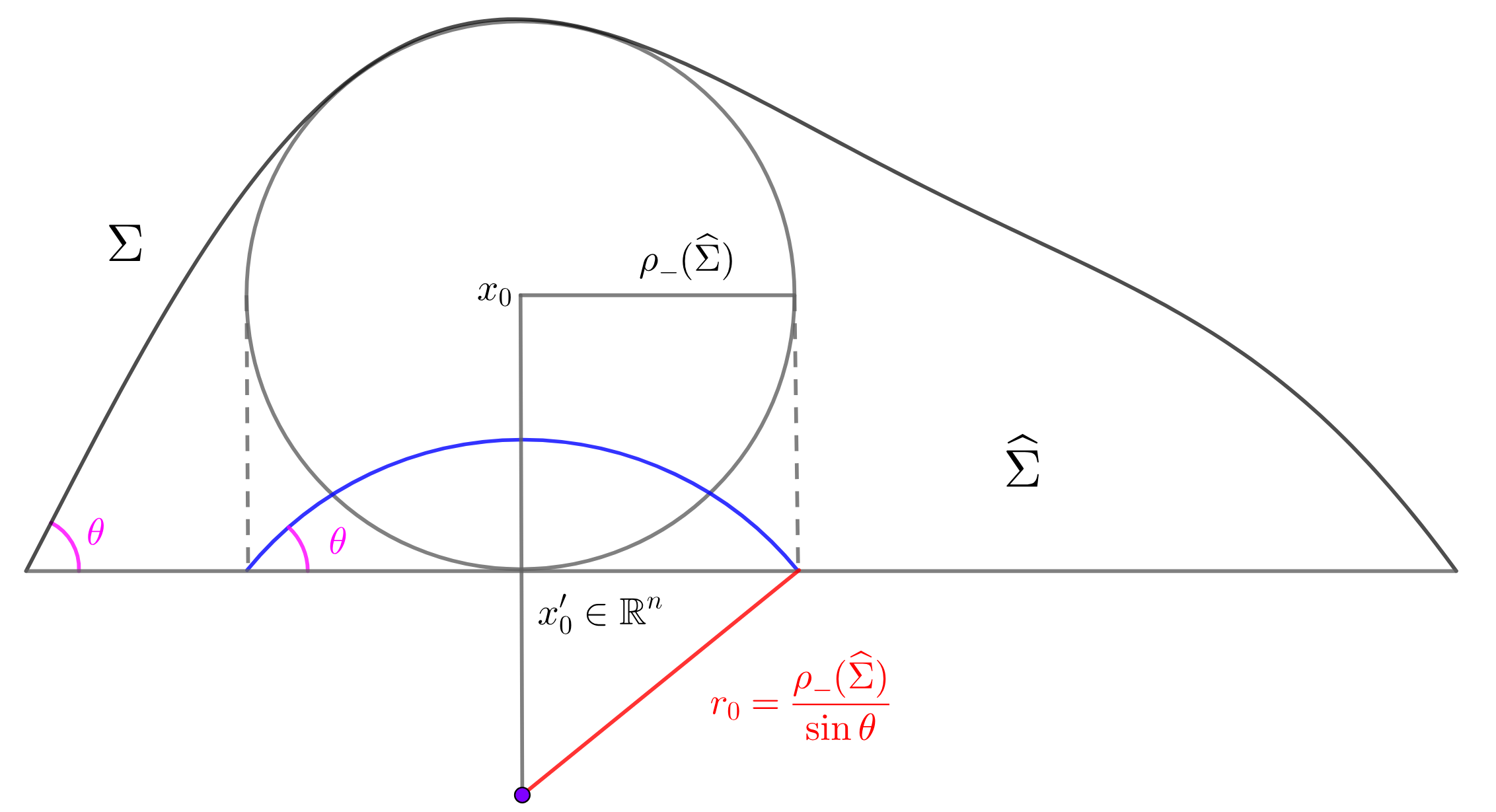
To obtain our result, we now have to show that the capillary radii are controlled by the classical ones. We start by estimating from below $\rho_{-}(\widehat{\Sigma},\theta)$ in terms of $\rho_{-}(\widehat{\Sigma})$. By definition, $\widehat{\Sigma}$ contains a ball $B_{0}$, centered at some point $x_{0}\in\mathbb{R}^{n+1}$ and of radius $\rho_{-}(\widehat{\Sigma})$. We denote by $B_{0}^{\prime}$ and $x_{0}^{\prime}$ the corresponding projections of $B_{0}$ and $x_{0}$ onto $\partial\mathbb{R}^{n+1}_{+}$. Observe that $B_{0}^{\prime}\subset\widehat{\partial\Sigma}$, by the convexity of $\Sigma$ and the condition $\theta\in(0,\frac{\pi}{2}]$. Let us now consider the spherical cap with angle $\theta$ having the same boundary as $B_{0}^{\prime}$, which is $\mathcal{C}_{r_{0},\theta}(x_{0}^{\prime})\subset\overline{\mathbb{R}^{n+1}_{+}}$ with $r_{0}=\frac{\rho_{-}(\widehat{\Sigma})}{\sin\theta}$. Then it is easy to see that $\widehat{\mathcal{C}_{r_{0},\theta}}\subset\widehat{\Sigma}$, see Figure 1. From the definition of capillary inner radius (2.20), we deduce

$\displaystyle\rho_{-}(\widehat{\Sigma},\theta)\geq r_{0}=\frac{\rho_{-}(\widehat{\Sigma})}{\sin\theta}.$ (2.26)
Refer to caption
Figure 1. Figure 1.

Let us now estimate $\rho_{+}(\widehat{\Sigma},\theta)$. Let $B_{0}$ be a ball of center $x_{0}$ and radius $\rho_{+}(\widehat{\Sigma})$ such that $\widehat{\Sigma}\subset\overline{B_{0}}$ and let again $x^{\prime}_{0}$ be the projection of $x_{0}$ onto $\partial\mathbb{R}^{n+1}_{+}$. Since $\widehat{\Sigma}\subset\overline{B_{0}}$ intersects $\partial\mathbb{R}^{n+1}_{+}$, the same does $B_{0}$, which implies $\rho_{+}(\widehat{\Sigma})\geq|x_{0}-x^{\prime}_{0}|$. If we now set

$$R=\frac{2\rho_{+}(\widehat{\Sigma})}{1-\cos\theta},$$

we see that any $x\in B_{0}$ satisfies

$\displaystyle|x-x_{0}^{\prime}+R\cos\theta E_{n+1}|$ $\displaystyle\leq$ $\displaystyle|x-x_{0}|+|x_{0}-x_{0}^{\prime}|+|R\cos\theta E_{n+1}|$
$\displaystyle\leq$ $\displaystyle\rho_{+}(\widehat{\Sigma})+\rho_{+}(\widehat{\Sigma})+R\cos\theta=R.$

This shows that $\overline{B_{0}}\subset\widehat{\mathcal{C}_{R,\theta}(x_{0}^{\prime})}$, which in turn implies

$\displaystyle\rho_{+}(\widehat{\Sigma},\theta)\leq R=\frac{2}{1-\cos\theta}\rho_{+}(\widehat{\Sigma}).$ (2.27)

In view of (2.26), (2.27) and (2.25), the proof of (2.24) is complete. ∎

3. A priori estimates

In this section, we establish the monotonicity of the capillary isoperimetric ratio $\mathcal{I}_{\theta}(\widehat{\Sigma_{t}})$ along our flow (1.8), and derive the curvature estimates. This will allow us to prove Theorem 1.1. Throughout the section, $\Sigma_{t}$ will be a smooth solution of the flow (1.8) with $\theta\in(0,\frac{\pi}{2})$, defined in its maximal time interval $[0,T^{*})$.

3.1. Monotonicity of capillary isoperimetric ratio

A key property of our flow (1.8) is that the capillary isoperimetric ratio (2.22) is monotone non-increasing in time. We remark that this property does not require the convexity of the surfaces and holds for a general $\theta\in(0,\pi)$.

Proposition 3.1.

Along the flow (1.8), the capillary isoperimetric ratio $\mathcal{I}_{\theta}(\widehat{\Sigma_{t}})$ is monotone non-increasing in time $t>0$. Moreover, monotonicity is strict unless $\Sigma_{t}$ is a spherical cap.

Proof.

Let us first look at the case that $\phi(t)$ is chosen as in (1.9). We have

$\displaystyle\frac{d}{dt}|\widehat{\Sigma_{t}}|=\int_{\Sigma_{t}}(\phi-H^{\alpha})(1-\cos\theta\langle\nu,E_{n+1}\rangle)dA=0.$

Let us denote

$$q(t):=\frac{\int_{\Sigma_{t}}H(1-\cos\theta\langle\nu,E_{n+1}\rangle)dA}{W_{\theta}(\widehat{\Sigma_{t}})}=\frac{\int_{\Sigma_{t}}H(1-\cos\theta\langle\nu,E_{n+1}\rangle)dA}{\int_{\Sigma_{t}}(1-\cos\theta\langle\nu,E_{n+1}\rangle)dA},$$

where we are using (1.4). Then the definitions immediately imply the identities

$$\phi(t)\int_{\Sigma_{t}}H(1-\cos\theta\langle\nu,E_{n+1}\rangle)dA=q(t)\int_{\Sigma_{t}}H^{\alpha}(1-\cos\theta\langle\nu,E_{n+1}\rangle)dA.$$
$$\int_{\Sigma_{t}}H(1-\cos\theta\langle\nu,E_{n+1}\rangle)dA-q(t)\int_{\Sigma_{t}}(1-\cos\theta\langle\nu,E_{n+1}\rangle)dA=0.$$

From the first variational formula in [53, Theorem 2.7], we deduce, using the two identities above,

$\displaystyle\frac{d}{dt}W_{\theta}(\widehat{\Sigma_{t}})$ $\displaystyle=$ $\displaystyle\int_{\Sigma_{t}}(\phi(t)-H^{\alpha})H(1-\cos\theta\langle\nu,E_{n+1}\rangle)dA$
$\displaystyle=$ $\displaystyle\int_{\Sigma_{t}}(q(t)H^{\alpha}-H^{\alpha+1})(1-\cos\theta\langle\nu,E_{n+1}\rangle)dA$
$\displaystyle+q^{\alpha}(t)\int_{\Sigma_{t}}H(1-\cos\theta\langle\nu,E_{n+1}\rangle)dA$
$\displaystyle-q^{\alpha+1}(t)\int_{\Sigma_{t}}(1-\cos\theta\langle\nu,E_{n+1}\rangle)dA$
$\displaystyle=$ $\displaystyle-\int_{\Sigma_{t}}(H-q(t))(H^{\alpha}-q^{\alpha}(t))(1-\cos\theta\langle\nu,E_{n+1}\rangle)dA$
$\displaystyle\leq$ $\displaystyle 0,$

where the last inequality follows from $\alpha>0$. Observe in addition that the last inequality is strict unless $H=q(t)$ everywhere om $\Sigma_{t}$, which means that $\Sigma_{t}$ is a spherical cap.

If $\phi(t)$ is chosen as in (1.10), we define $q(t)$ as above and we obtain this time

$$\phi(t)\int_{\Sigma_{t}}(1-\cos\theta\langle\nu,E_{n+1}\rangle)dA=\frac{1}{q(t)}\int_{\Sigma_{t}}H^{\alpha+1}(1-\cos\theta\langle\nu,E_{n+1}\rangle)dA.$$

Using again [53, Theorem 2.7] we obtain, with computations similar to the previous case,

$\displaystyle\frac{d}{dt}W_{\theta}(\widehat{\Sigma_{t}})=0,$

and

$\displaystyle\frac{d}{dt}|\widehat{\Sigma_{t}}|$ $\displaystyle=$ $\displaystyle\int_{\Sigma_{t}}(\phi-H^{\alpha})(1-\cos\theta\langle\nu,E_{n+1}\rangle)dA$
$\displaystyle=$ $\displaystyle\frac{1}{q(t)}\int_{\Sigma_{t}}(H-q(t))(H^{\alpha}-q^{\alpha}(t))(1-\cos\theta\langle\nu,E_{n+1}\rangle)dA$
$\displaystyle\geq$ $\displaystyle 0.$

In both cases, we conclude that $\mathcal{I}_{\theta}(\widehat{\Sigma_{t}})$ is monotone non-increasing in $t$. ∎

3.2. Curvature estimates

Now we prove that the convexity is preserved along our flow (1.8).

Proposition 3.2.

If $\Sigma_{0}\subset\overline{\mathbb{R}^{n+1}_{+}}$ is a strictly convex capillary hypersurface and $\theta\in(0,\frac{\pi}{2})$, then the solution $\Sigma_{t}$ of flow (1.8) is strictly convex for all $t\in[0,T^{*})$.

To demonstrate Proposition 3.2, we begin by recalling the following tensor maximum principle from [26, Theorem 1.2], which is a refinement of the result by Stahl [50, Theorem 3.3]. Both can be regarded as the boundary counterpart of the tensor maximum principle on a compact manifold established by Hamilton [25, Theorem 9.1] and further refinement by Andrews [4, Theorem 3.2].

Lemma 3.3 ([26]).

Let $N$ be a compact manifold with boundary and $g$ a time-dependent metric. Let $S(t)$ be a smooth symmetric $(2,0)$-tensor field satisfying

$\displaystyle\frac{\partial}{\partial t}S=A^{ij}\nabla_{i}\nabla_{j}S+B^{k}\nabla_{k}S+\beta,$

where $(A^{ij})>0$ and $B^{k}$ are smooth. Suppose $\beta(t)=\beta(S(t),g(t),t)$ is a symmetric $(2,0)$ tensor which satisfies

$\displaystyle\beta(\xi,\xi)+\sup\limits_{\Lambda}2A^{kl}(2\Lambda^{p}_{k}\nabla_{l}S_{ip}\xi^{i}-\Lambda^{p}_{k}\Lambda^{q}_{l}S_{pq})\geq 0,\leavevmode\nobreak\ \leavevmode\nobreak\ \text{ in }N\times(0,T],$ (3.1)

and

$\displaystyle(\nabla_{\mu}S_{ij})\xi^{i}\xi^{j}\geq 0,\leavevmode\nobreak\ \leavevmode\nobreak\ \text{ on }\partial N\times(0,T],$ (3.2)

for $\xi$ being a null eigenvector of $S$, i.e. $S_{ij}\xi^{j}=0$ and $\mu$ being the outward unit normal vector to $\partial N$. If $S(0)>0$ on $N$, then $S(t)>0$ on $N$ for all $0<t\leq T$.

Proof of Proposition 3.2.

From Proposition 2.1 (3), we have

$\displaystyle\partial_{t}h_{ij}$ $\displaystyle=$ $\displaystyle-\nabla_{i}\nabla_{j}(f(1-\cos\theta\langle\nu,E_{n+1}\rangle))+f(1-\cos\theta\langle\nu,E_{n+1}\rangle)(h^{2})_{ij}$
$\displaystyle+\nabla_{\mathcal{T}}h_{ij}+h_{j}^{k}\nabla_{i}\mathcal{T}_{k}+h_{i}^{k}\nabla_{j}\mathcal{T}_{k}$
$\displaystyle=$ $\displaystyle(1-\cos\theta\langle\nu,E_{n+1}\rangle)\nabla_{i}\nabla_{j}H^{\alpha}+\nabla_{i}H^{\alpha}\nabla_{j}(1-\cos\theta\langle\nu,E_{n+1}\rangle)$
$\displaystyle+\nabla_{j}H^{\alpha}\nabla_{i}(1-\cos\theta\langle\nu,E_{n+1}\rangle)-(\phi-H^{\alpha})\nabla_{ij}(1-\cos\theta\langle\nu,E_{n+1}\rangle)$
$\displaystyle+(1-\cos\theta\langle\nu,E_{n+1}\rangle)(\phi-H^{\alpha})(h^{2})_{ij}+\nabla_{\mathcal{T}}h_{ij}+h_{j}^{k}\nabla_{i}\mathcal{T}_{k}+h_{i}^{k}\nabla_{j}\mathcal{T}_{k}$
$\displaystyle=$ $\displaystyle\alpha(1-\cos\theta\langle\nu,E_{n+1}\rangle)(H^{\alpha-1}H_{;ij}+(\alpha-1)H^{\alpha-2}H_{;i}H_{;j})$
$\displaystyle-\alpha\cos\theta H^{\alpha-1}(H_{;i}h_{jk}\langle e_{k},E_{n+1}\rangle+H_{;j}h_{ik}\langle e_{k},E_{n+1}\rangle)$
$\displaystyle+(\phi-H^{\alpha})\cos\theta(\langle\nabla h_{ij},E_{n+1}\rangle-(h^{2})_{ij}\langle\nu,E_{n+1}\rangle)$
$\displaystyle+(1-\cos\theta\langle\nu,E_{n+1}\rangle)(\phi-H^{\alpha})(h^{2})_{ij}+\nabla_{\mathcal{T}}h_{ij}+h_{j}^{k}\nabla_{i}\mathcal{T}_{k}+h_{i}^{k}\nabla_{j}\mathcal{T}_{k}.$

We recall the Simons-type identity, see e.g. [27, Lemma 2.1].

$\displaystyle H_{;ij}=\Delta h_{ij}-H(h^{2})_{ij}+|h|^{2}h_{ij}.$

Then we derive

$\displaystyle\partial_{t}h_{ij}$ $\displaystyle=$ $\displaystyle\alpha(1-\cos\theta\langle\nu,E_{n+1}\rangle)H^{\alpha-1}\Delta h_{ij}+(\phi-H^{\alpha})\cos\theta\langle\nabla h_{ij},E_{n+1}\rangle$
$\displaystyle+\nabla_{\mathcal{T}}h_{ij}+\alpha(\alpha-1)(1-\cos\theta\langle\nu,E_{n+1}\rangle)H^{\alpha-2}H_{;i}H_{;j}$
$\displaystyle-\alpha\cos\theta H^{\alpha-1}(H_{;i}h_{jk}\langle e_{k},E_{n+1}\rangle+H_{;j}h_{ik}\langle e_{k},E_{n+1}\rangle)$
$\displaystyle+(1-2\cos\theta\langle\nu,E_{n+1}\rangle)(\phi-H^{\alpha})(h^{2})_{ij}+h_{j}^{k}\nabla_{i}\mathcal{T}_{k}+h_{i}^{k}\nabla_{j}\mathcal{T}_{k}$
$\displaystyle+\alpha(1-\cos\theta\langle\nu,E_{n+1}\rangle)H^{\alpha-1}(|h|^{2}h_{ij}-H(h^{2})_{ij}).$

To apply Lemma 3.3, we first check the boundary condition (3.2). Assume that $h_{ij}\geq 0$ and $h_{ij}\xi^{j}=0$ holds at the point $p_{0}\in\partial M$. We choose an orthonormal frame $\{e_{i}\}_{i=1}^{n}$ around $p_{0}$ such that $e_{1}=\mu$ is the conormal of $\partial M$ in $M$. Recalling (2.5), we can choose our frame in such a way that one of the following holds: either $\xi=e_{1}$ or $\xi=e_{\alpha}\in T(\partial\Sigma_{t})$ for some $2\leq\alpha\leq n$.

  1. (1)

    If $\xi=\mu$, we know $h_{\alpha\alpha}\geq h_{11}$ for all $2\leq\alpha\leq n$. From (2.19), we know

    $\displaystyle\nabla_{\mu}h_{11}=-\sum_{\alpha=2}^{n}\nabla_{\mu}h_{\alpha\alpha}.$

    By applying [53, Proposition 2.4] and using $\theta\in(0,\frac{\pi}{2})$, we obtain

    $\displaystyle(\nabla_{\mu}h_{ij})\xi^{i}\xi^{j}=\nabla_{\mu}h_{11}=-\sum_{\alpha=2}^{n}\cot\theta\,h_{\alpha\alpha}(h_{11}-h_{\alpha\alpha})\geq 0.$ (3.3)
  2. (2)

    If $\xi=e_{\alpha}\in T(\partial\Sigma_{t})$ for some $2\leq\alpha\leq n$, then $h_{11}\geq h_{\alpha\alpha}$, we use again [53, Proposition 2.4] and $\theta\in(0,\frac{\pi}{2})$ to deduce that

    $\displaystyle(\nabla_{\mu}h_{ij})\xi^{i}\xi^{j}=\nabla_{\mu}h_{\alpha\alpha}=\cot\theta\,h_{\alpha\alpha}(h_{11}-h_{\alpha\alpha})\geq 0.$ (3.4)

Next, we check condition (3.1). We assume that $\xi$ is a null eigenvector of $(h_{ij})\geq 0$, i.e. $h_{ij}\xi^{j}=0$ at the point $(p_{0},t_{0})$ with $p_{0}\in M\setminus\partial M$. We choose an orthonormal frame $\{e_{i}\}_{i=1}^{n}$ around $p_{0}$ such that $(h_{ij})$ is diagonal and $\xi=e_{1}$, then $h_{11}=0$ and $(h^{2})_{11}=\sum\limits_{k=1}^{n}h_{1}^{k}h_{k}^{1}=0$. Then many terms in the evolution equation for $h_{ij}$ vanish and we find that condition (3.1) in our case takes the following form

$\displaystyle Q$ $\displaystyle:=$ $\displaystyle\alpha(\alpha-1)(1-\cos\theta\langle\nu,E_{n+1}\rangle)H^{\alpha-2}(\nabla_{1}H)^{2}$
$\displaystyle+2\alpha(1-\cos\theta\langle\nu,E_{n+1}\rangle)H^{\alpha-1}\sup_{\Lambda}(2\Lambda_{k}^{l}\nabla_{k}h_{l1}-\Lambda_{k}^{i}\Lambda_{k}^{j}h_{ij})$
$\displaystyle\geq$ $\displaystyle 0.$

Here we no longer distinguish between upper and lower indices since we are working in an orthonormal frame.

If $\alpha\geq 1$, it is easy to see that $Q\geq 0$, by choosing $\Lambda\equiv 0$ in (3.2). Hence we only need to show (3.2) for $\alpha\in(0,1)$. By continuity, we can assume that $(h_{ij})$ has all eigenvalues $\{\kappa_{i}\}_{i=1}^{n}$ distinct and in increasing order at $(p_{0},t_{0})$ as $\kappa_{1}<\kappa_{2}<\cdots<\kappa_{n}$. From the minimality of $\kappa_{1}=h_{11}$ (cf. [26, Lemma 4.1], we have that $0=\nabla_{k}h_{11}$ for all $1\leq k\leq n$. By choosing $\Lambda_{k}^{l}=\frac{\nabla_{1}h_{kl}}{h_{ll}}$ for $2\leq l\leq n,1\leq k\leq n$ and $\Lambda^{1}_{k}\equiv 0$ for $1\leq k\leq n$, we have

$\displaystyle 2\Lambda_{k}^{l}\nabla_{1}h^{k}_{l}-\Lambda_{k}^{i}\Lambda^{jk}h_{ij}$
$\displaystyle=$ $\displaystyle\sum_{l=2}^{n}\sum_{k=1}^{n}\left(2\frac{\nabla_{1}h_{kl}}{h_{ll}}\nabla_{1}h_{kl}-\left(\frac{\nabla_{1}h_{kl}}{h_{ll}}\right)^{2}h_{ll}\right)$
$\displaystyle=$ $\displaystyle\sum_{l=2}^{n}\sum_{k=1}^{n}\frac{(\nabla_{1}h_{kl})^{2}}{h_{ll}}\geq\sum_{l=2}^{n}\frac{(\nabla_{1}h_{ll})^{2}}{h_{ll}}\geq\frac{(\nabla_{1}H)^{2}}{H},$

where in the last step we have used the Cauchy-Schwarz inequality

$\displaystyle|\nabla_{1}H|=\left|\sum_{l=2}^{n}\frac{\nabla_{1}h_{ll}}{\sqrt{h_{ll}}}\,\sqrt{h_{ll}}\,\right|\leq\left(\sum_{l=2}^{n}\frac{(\nabla_{1}h_{ll})^{2}}{h_{ll}}\right)^{1/2}H^{1/2}.$

Substituting into (3.2), it implies

$\displaystyle Q$ $\displaystyle\geq$ $\displaystyle\alpha(1-\cos\theta\langle\nu,E_{n+1}\rangle)H^{\alpha-2}\left[(\alpha-1)(\nabla_{1}H)^{2}+2{(\nabla_{1}H)^{2}}\right]$
$\displaystyle=$ $\displaystyle\alpha(\alpha+1)(1-\cos\theta\langle\nu,E_{n+1}\rangle)H^{\alpha-2}(\nabla_{1}H)^{2}\geq 0,$

that is, (3.2) holds also in this case. In summary, the theorem follows by using Lemma 3.3. ∎

Proposition 3.4.

Along the flow (1.8), if $\theta\in(0,\frac{\pi}{2})$, the enclosed volume $|\widehat{\Sigma_{t}}|$, the capillary area $W_{\theta}(\widehat{\Sigma_{t}})$, the capillary outer radius $\rho_{+}(\widehat{\Sigma_{t}},\theta)$ and the capillary inner radius $\rho_{-}(\widehat{\Sigma_{t}},\theta)$ are uniformly bounded from above and below by positive constants. In particular, there exist positive constants $R_{0}$ and $r_{0}$, depending only on the initial datum, such that

$\displaystyle 0<r_{0}\leq\rho_{-}(\widehat{\Sigma_{t}},\theta)\leq\rho_{+}(\widehat{\Sigma_{t}},\theta)\leq R_{0}.$ (3.6)
Proof.

From Proposition 3.1 and (2.23), we have

$\displaystyle\mathcal{I}_{\theta}(\widehat{\mathcal{C}_{\theta}})\leq\mathcal{I}_{\theta}(\widehat{\Sigma_{t}})\leq\mathcal{I}_{\theta}(\widehat{\Sigma_{0}}),$ (3.7)

for all $t>0$.

If $\phi(t)$ is chosen as in (1.9), we have

$$|\widehat{\Sigma_{t}}|=|\widehat{\Sigma_{0}}|,$$

for all $t\geq 0$, then the uniform bounds on the capillary area $W_{\theta}(\widehat{\Sigma_{t}})$ follow from (3.7). In addition, from (3.7) and Proposition 2.4 we deduce

$\displaystyle|\widehat{\Sigma_{t}}|$ $\displaystyle\leq$ $\displaystyle|\widehat{\mathcal{C}_{\rho_{+}({\widehat{\Sigma_{t}}},\theta),\theta}}|=(\rho_{+}({\widehat{\Sigma_{t}},\theta}))^{n+1}|\widehat{\mathcal{C}_{\theta}}|$
$\displaystyle\leq$ $\displaystyle(c\rho_{-}({\widehat{\Sigma_{t}},\theta}))^{n+1}|\widehat{\mathcal{C}_{\theta}}|\leq c^{n+1}|\widehat{\Sigma_{t}}|.$

Since $|\widehat{\Sigma_{t}}|$ is constant in time, this implies the uniform bounds on $\rho_{\pm}({\widehat{\Sigma_{t}}},\theta)$.

In the case that $\phi(t)$ is chosen as in (1.10), we know that

$\displaystyle W_{\theta}(\widehat{\Sigma_{t}})=W_{\theta}(\widehat{\Sigma_{0}}),$

for all $t\geq 0$. From Proposition 3.1 and (3.7), we have

$$|\widehat{\Sigma_{0}}|\leq|\widehat{\Sigma_{t}}|=\mathcal{I}_{\theta}(\widehat{\Sigma_{t}})^{-\frac{1}{n}}W_{\theta}(\widehat{\Sigma_{t}})^{\frac{n+1}{n}}\leq\mathcal{I}_{\theta}(\widehat{\mathcal{C}_{\theta}})^{-\frac{1}{n}}W_{\theta}(\widehat{\Sigma_{0}})^{\frac{n+1}{n}},$$

showing that $|\widehat{\Sigma_{t}}|$ is uniformly bounded. The remaining quantities can be estimated similarly as above. ∎

Proposition 3.4 implies the existence of a capillary spherical cap with radius $r_{0}$ contained within $\widehat{\Sigma_{t}}$ for any $t\in[0,T^{*})$. The center of the cap, however, may in principle depend on $t$. To use Tso’s method [51] for obtaining an upper bound on the mean curvature, it is necessary to establish the existence of a cap with a fixed center that remains inside $\widehat{\Sigma_{t}}$ over a suitable uniform time interval. This is done in the next lemma, by adapting a technique from [3, 36].

Lemma 3.5.

Let $\Sigma_{t}$ be the solution of (1.8). For any $s\geq 0$, let $z_{*}\in\widehat{\Sigma_{s}}\cap\partial\mathbb{R}^{n+1}_{+}$ be a point such that $\widehat{\mathcal{C}_{r_{0},\theta}(z_{*})}\subset\widehat{\Sigma_{s}}$, with $r_{0}$ as in (3.6). Then there exists some $\tau_{0}>0$, which only depends on the initial datum, such that $\Sigma_{t}$ satisfies

$\displaystyle\widehat{\mathcal{C}_{\frac{r_{0}}{2},\theta}(z_{*})}\subset\widehat{\Sigma_{t}}$ (3.8)

for all $t\in[s,\min\{s+\tau_{0},T^{*}\})$.

Proof.

The idea of the proof is to compare $\Sigma_{t}$ with the capillary spherical cap centered at $z_{*}-r(t)\cos\theta E_{n+1}$ with shrinking radius $r(t)$, where $r(t)$ satisfies

$\displaystyle r^{\prime}(t)=-\left(\frac{n}{r(t)}\right)^{\alpha},$ (3.9)

with $r(s)=\frac{99}{100}r_{0}$. We define

$\displaystyle F(t):=\frac{1}{2}\left(\min_{M}|X(\cdot,t)-(z_{*}-r(t)\cos\theta E_{n+1})|^{2}-r^{2}(t)\right),$

for any $t\geq s$ such that $\Sigma_{t}$ and $r(t)$ exist. It is easy to see that $F(s)>0$. The conclusion (3.8) will follow easily once we show that $F(t)>0$ for $t>s$.

Suppose $t_{0}>s$ be the first time such that $F(t)=0$, and let $p_{0}\in M$ be a minimum value point of

$$|X(p_{0},t_{0})-(z_{*}-r(t_{0})\cos\theta E_{n+1})|=\min_{M}|X(\cdot,t_{0})-(z_{*}-r(t_{0})\cos\theta E_{n+1})|=r(t_{0}).$$

Next we divide the proof into two cases: $p_{0}\in\mathring{M}$ and $p_{0}\in\partial M$.

  1. (1)

    $p_{0}\in\mathring{M}$. Then at $p_{0}$ we have

    $\displaystyle\nu=\frac{X-(z_{*}-r(t_{0})\cos\theta E_{n+1})}{|X-(z_{*}-r(t_{0})\cos\theta E_{n+1})|}=\frac{X-(z_{*}-r(t_{0})\cos\theta E_{n+1})}{r(t_{0})},$ (3.10)

    which also implies

    $\displaystyle\widetilde{\nu}=\nu-\cos\theta E_{n+1}=\frac{X(p_{0},t_{0})-z_{*}}{r(t_{0})}.$ (3.11)

    Moreover, the spherical cap $\mathcal{C}_{r(t_{0}),\theta}(z_{*}-r(t_{0})\cos\theta E_{n+1})$ is tangent to $\Sigma_{t_{0}}$ at $X(p_{0},t_{0})$ from the interior. It follows that the principal curvatures $\kappa_{i}$ of $\Sigma_{t_{0}}$ satisfy

    $\displaystyle\kappa_{i}(p_{0},t_{0})\leq\frac{1}{r(t_{0})},\leavevmode\nobreak\ \leavevmode\nobreak\ \forall\leavevmode\nobreak\ 1\leq i\leq n.$

    Then

    $\displaystyle H(p_{0},t_{0})\leq\frac{n}{r(t_{0})}.$ (3.12)
  2. (2)

    $p_{0}\in\partial M$. By (2.5), if we choose $\{e_{\alpha}\}_{\alpha=1}^{n-1}$ to be an orthonormal frame on $T\partial\Sigma_{t_{0}}\subset T\mathbb{R}^{n}$ and set $e_{n}:=\mu$, then $\{e_{i}\}_{i=1}^{n}$ is an orthonormal frame on $T\Sigma_{t_{0}}$. From [53, Proposition 2.4 (2)], we know

    $\displaystyle\kappa_{\alpha}=\sin\theta\,\widehat{\kappa}_{\alpha},$ (3.13)

    where $\{\widehat{\kappa}_{\alpha}\}_{\alpha=1}^{n-1}$ are the principal curvatures of $\partial\Sigma_{t}$ in $\partial\mathbb{R}^{n+1}_{+}=\mathbb{R}^{n}$.

    By definition of $p_{0}$, we have that

    $\displaystyle|X(p_{0},t_{0})-(z_{*}-r(t_{0})\cos\theta E_{n+1})|^{2}$
    $\displaystyle=$ $\displaystyle\min_{M}|X(\cdot,t_{0})-(z_{*}-r(t_{0})\cos\theta E_{n+1})|^{2}$
    $\displaystyle=$ $\displaystyle\min_{\partial M}|X(\cdot,t_{0})-(z_{*}-r(t_{0})\cos\theta E_{n+1})|^{2}.$

    On the other hand, for all $p\in\partial M$ we have

    $$\qquad\qquad|X(p,t_{0})-z_{*}+r(t_{0})\cos\theta E_{n+1}|^{2}=|X(p,t_{0})-z_{*}|^{2}+r^{2}(t_{0})\cos^{2}\theta.$$

    It follows that $p_{0}$ attains the minimal value of $\min\limits_{\partial M}|X(\cdot,t_{0})-z_{*}|^{2}$. Then we have that the horizontal component of $\nu$ is parallel to $X-z_{*}$ at $p_{0}$. In addition, if we regard $\partial\Sigma_{t_{0}}$ as a subset of $\partial\mathbb{R}^{n+1}_{+}=\mathbb{R}^{n}$, we have that the $n$-dimensional ball $B_{|X(p_{0},t_{0})-z_{*}|}^{n}(z_{*})\subset\partial\mathbb{R}^{n+1}_{+}$ is tangent to $\partial\Sigma_{t_{0}}$ from the inside at $X(p_{0},t_{0})$. This yields

    $\displaystyle\widehat{\kappa}_{\alpha}\leq\frac{1}{|X(p_{0},t_{0})-z_{*}|},\quad\forall\leavevmode\nobreak\ 1\leq\alpha\leq n-1,$ (3.14)

    and

    $\displaystyle\widetilde{\nu}=\frac{|\widetilde{\nu}|}{|X-z_{*}|}(X-z_{*})=\frac{|\nu-\cos\theta E_{n+1}|}{r(t_{0})\sin\theta}(X-z_{*})=\frac{X-z_{*}}{r(t_{0})},$ (3.15)

    where the last equality used (1.3). That is, (3.11) holds in this case, and also (3.10). Furthermore, from (3.15), we have

    $\displaystyle\langle\mu,X-z_{*}+r\cos\theta E_{n+1}\rangle=r(t_{0})\langle\mu,\nu\rangle=0,$

    that is, $\mu$ is tangent to the spherical cap centred at $X-z_{*}+r\cos\theta E_{n+1}$ with radius $r(t_{0})$, and this implies that

    $\displaystyle h(\mu,\mu)\leq\frac{1}{r(t_{0})}.$ (3.16)

    In view of (3.14), (3.13) and $|X(p_{0},t_{0})-z_{*}|=r(t_{0})\sin\theta$, we have

    $\displaystyle\kappa_{\alpha}\leq\frac{1}{r(t_{0})},\leavevmode\nobreak\ \leavevmode\nobreak\ \forall\leavevmode\nobreak\ 1\leq\alpha\leq n-1.$

    Together with (3.16), we conclude that (3.12) holds also in this case.

In the following we use standard properties about the derivative of the minimum of a family of smooth functions; we also assume for simplicity that $F$ is differentiable at $t=t_{0}$, since the argument can be extended to the general case by using Dini derivatives.

We have seen that, in both cases, we have (3.10), (3.11) and (3.12). Taking also into account (3.9), we compute

$\displaystyle\left.\frac{d}{dt}F(t)\right|_{t=t_{0}}$ $\displaystyle=$ $\displaystyle\langle X-z_{*}+r\cos\theta E_{n+1},\partial_{t}X+r^{\prime}(t_{0})\cos\theta E_{n+1}\rangle-rr^{\prime}(t_{0})$
$\displaystyle=$ $\displaystyle\left\langle r\nu,(\phi-H^{\alpha})\frac{X-z_{*}}{r}+r^{\prime}(t_{0})\left(\nu-\frac{X-z_{*}}{r}\right)\right\rangle-rr^{\prime}(t_{0})$
$\displaystyle=$ $\displaystyle(\phi-H^{\alpha})\langle X-z_{*},\nu\rangle-r^{\prime}(t_{0})\langle X-z_{*},\nu\rangle$
$\displaystyle>$ $\displaystyle\langle X-z_{*},\nu\rangle\left[-H^{\alpha}+\left(\frac{n}{r(t_{0})}\right)^{\alpha}\right]\geq 0,$

which contradicts the definition of $t_{0}$. This shows that $F(t)$ cannot vanish and therefore remains positive for $t>s$. Now it suffices to choose $\tau_{0}>0$ such that $r(t)\geq\frac{r_{0}}{2}$ for all $t\in[s,s+\tau_{0})$. Note that from (3.9), we know $\tau_{0}$ only depends on $r_{0}$, hence only on the initial datum. Then we have $F(t)>0$ for all $t\in[s,\min\{s+\tau_{0},T^{*}\})$. This completes the proof.

We can now prove a uniform upper bound for the curvature of our flow.

Proposition 3.6.

If $\Sigma_{t}$ be a solution of the flow (1.8), there holds

$\displaystyle H\leq C\mbox{ on }\Sigma_{t},\leavevmode\nobreak\ \leavevmode\nobreak\ \leavevmode\nobreak\ \forall\leavevmode\nobreak\ t\in[0,T^{*}),$ (3.17)

where $C$ is a positive constant, only depending on the initial datum.

Proof.

For any given $s\in[0,T^{*})$, let $z_{*}$ and $\tau_{0}$ be chosen as in Lemma 3.5. Then (3.8) and the convexity of $\Sigma_{t}$ imply

$$\langle X-z_{*}+\frac{r_{0}}{2}\cos\theta E_{n+1},\nu\rangle\geq\frac{r_{0}}{2},$$

showing that the capillary support function satisfies

$\displaystyle\bar{u}:=\frac{\langle X-z_{*},\nu\rangle}{1-\cos\theta\langle\nu,E_{n+1}\rangle}\geq\frac{r_{0}}{2}>0,\leavevmode\nobreak\ \leavevmode\nobreak\ \leavevmode\nobreak\ \forall\leavevmode\nobreak\ t\in[s,\min\{s+\tau_{0},T^{*}\}).$

We denote $\varepsilon:=\frac{r_{0}}{4}$, so that $\bar{u}-\varepsilon\geq\varepsilon>0$, and introduce the function

$\displaystyle\Phi:=\frac{H^{\alpha}}{\bar{u}-\varepsilon}.$ (3.18)

From Proposition 2.3, we deduce that

$\displaystyle\mathcal{L}H^{\alpha}=-\alpha H^{\alpha-1}(\phi-H^{\alpha})|h|^{2}+2\alpha H^{\alpha-1}\langle\nabla H^{\alpha},\nabla(1-\cos\theta\langle\nu,E_{n+1}\rangle)\rangle.$ (3.19)

Combining (2.9) and (3.19), we obtain

$\displaystyle\mathcal{L}\Phi$ $\displaystyle=$ $\displaystyle\frac{\mathcal{L}H^{\alpha}}{\bar{u}-\varepsilon}-\frac{H^{\alpha}\mathcal{L}\bar{u}}{(\bar{u}-\varepsilon)^{2}}+\frac{2\alpha H^{\alpha-1}}{\bar{u}-\varepsilon}(1-\cos\theta\langle\nu,E_{n+1}\rangle)\langle\nabla\Phi,\nabla\bar{u}\rangle$
$\displaystyle=$ $\displaystyle\frac{1}{\bar{u}-\varepsilon}(-\alpha H^{\alpha-1}f|h|^{2}+2\alpha H^{\alpha}\langle\nabla H^{\alpha},\nabla(1-\cos\theta\langle\nu,E_{n+1}\rangle)\rangle)$
$\displaystyle-\frac{\Phi}{\bar{u}-\varepsilon}\left[\phi-(1+\alpha)H^{\alpha}+\alpha\bar{u}H^{\alpha-1}|h|^{2}\right]$
$\displaystyle-\frac{2\alpha H^{\alpha-1}\Phi}{\bar{u}-\varepsilon}\left\langle\nabla\bar{u},\nabla(1-\cos\theta\langle\nu,E_{n+1}\rangle)\right\rangle$
$\displaystyle+\frac{2\alpha H^{\alpha-1}}{\bar{u}-\varepsilon}(1-\cos\theta\langle\nu,E_{n+1}\rangle)\langle\nabla\Phi,\nabla\bar{u}\rangle$
$\displaystyle=$ $\displaystyle-(\alpha H^{\alpha-1}|h|^{2}+\Phi)\frac{\phi}{\bar{u}-\varepsilon}-\frac{\varepsilon\alpha H^{2\alpha-1}|h|^{2}}{(\bar{u}-\varepsilon)^{2}}+(1+\alpha)\Phi^{2}$
$\displaystyle+2\alpha H^{\alpha-1}\langle\nabla\Phi,\nabla(1-\cos\theta\langle\nu,E_{n+1}\rangle)\rangle+\frac{2\alpha\varphi H^{\alpha-1}}{\bar{u}-\varepsilon}\langle\nabla\Phi,\nabla\bar{u}\rangle$
$\displaystyle\leq$ $\displaystyle-\frac{\varepsilon\alpha H^{2\alpha-1}|h|^{2}}{(\bar{u}-\varepsilon)^{2}}+(1+\alpha)\Phi^{2},\leavevmode\nobreak\ \leavevmode\nobreak\ \leavevmode\nobreak\ \text{ mod }\nabla\Phi,$

where we have used that $\phi>0$ by the convexity of $\Sigma_{t}$. Using also

$$|h|^{2}\geq\frac{H^{2}}{n},$$

we conclude that

$\displaystyle\mathcal{L}\Phi\leq-\frac{\alpha}{n}\varepsilon^{1+\frac{1}{\alpha}}\Phi^{2+\frac{1}{\alpha}}+(1+\alpha)\Phi^{2}\leavevmode\nobreak\ \leavevmode\nobreak\ \leavevmode\nobreak\ \text{ mod }\nabla\Phi,$ (3.20)

holds on $t\in[s,\min\{s+\tau_{0},T^{*}\})$.

On $\partial M$, by (2.15) and (2.11) we have

$\displaystyle\nabla_{\mu}\Phi=\frac{\nabla_{\mu}H^{\alpha}}{\bar{u}-\varepsilon}-\frac{H^{\alpha}\nabla_{\mu}\bar{u}}{(\bar{u}-\varepsilon)^{2}}=0.$ (3.21)

By the Hopf boundary point lemma, this shows that $\Phi$ attains its maximum value either at $t=0$ or at some interior point, say $p_{0}\in\mathring{M}$. We define

$$\widetilde{\Phi}(t):=\sup_{M}\Phi(p,t).$$

From (3.20), we know $\widetilde{\Phi}$ satisfies

$\displaystyle\frac{d}{dt}\widetilde{\Phi}(t)\leq\widetilde{\Phi}^{2}\left(1+\alpha-\frac{\alpha}{n}\varepsilon^{1+\frac{1}{\alpha}}\widetilde{\Phi}^{\frac{1}{\alpha}}\right),\leavevmode\nobreak\ \leavevmode\nobreak\ \leavevmode\nobreak\ \text{ a.e. }t\in[s,\max\{s+\tau_{0},T^{*}\}).$ (3.22)

In the case $s=0$, we argue as follows. From (3.22) we see that, if $\widetilde{\Phi}>\left(\frac{2n(1+\alpha)}{\alpha\varepsilon^{1+\frac{1}{\alpha}}}\right)^{\alpha}$ at some time, then it does not increase. This implies

$\displaystyle\Phi(\cdot,t)\leq\max\left\{\max_{M}\Phi(\cdot,0),\left(\frac{2n(1+\alpha)}{\alpha\varepsilon^{1+\frac{1}{\alpha}}}\right)^{\alpha}\right\},$

for $t\in\left[0,\min\left\{\tau_{0},T^{*}\right\}\right)$. Together with Proposition 3.4, this yields

$\displaystyle H(\cdot,t)\leq\frac{R_{0}^{\frac{1}{\alpha}}}{\varepsilon}\max\left\{\max_{M}H(\cdot,0),\frac{2(1+\alpha)}{\alpha\varepsilon^{\frac{1}{\alpha}}}\right\},$ (3.23)

for $t\in\left[0,\min\left\{\tau_{0},T^{*}\right\}\right)$.

Now we take any $s>0$ and deduce from (3.22) that, whenever $\widetilde{\Phi}>\left(\frac{2n(1+\alpha)}{\alpha\varepsilon^{1+\frac{1}{\alpha}}}\right)^{\alpha}$, we have

$\displaystyle\frac{d}{dt}\widetilde{\Phi}\leq-(1+\alpha)\widetilde{\Phi}^{2},\leavevmode\nobreak\ \leavevmode\nobreak\ \text{ a.e. }t\in[s,\max\{s+\tau_{0},T^{*}\}).$

This implies

$\displaystyle\widetilde{\Phi}(t)\leq\frac{1}{\widetilde{\Phi}^{-1}(s)+(1+\alpha)(t-s)}\leq\frac{1}{(1+\alpha)(t-s)},$

thus it follows

$\displaystyle\Phi(\cdot,t)\leq\max\left\{\left(\frac{2n(1+\alpha)}{\alpha\varepsilon^{1+\frac{1}{\alpha}}}\right)^{\alpha},\frac{1}{(1+\alpha)(t-s)}\right\},$

for $t\in[s,\min\{s+\tau_{0},T^{*}\})$. In particular, if $t>s+\frac{\tau_{0}}{2}$, we obtain

$\displaystyle\Phi(\cdot,t)\leq\max\left\{\left(\frac{2n(1+\alpha)}{\alpha\varepsilon^{1+\frac{1}{\alpha}}}\right)^{\alpha},\frac{2}{(1+\alpha)\tau_{0}}\right\},$

and so

$\displaystyle H(\cdot,t)\leq R_{0}^{\frac{1}{\alpha}}\max\left\{\frac{2n(1+\alpha)}{\alpha\varepsilon^{1+\frac{1}{\alpha}}},\left(\frac{2}{(1+\alpha)\tau_{0}}\right)^{\frac{1}{\alpha}}\right\},$ (3.24)

for $t\in[s+\frac{\tau_{0}}{2},\min\{s+\tau_{0},T^{*}\})$. Since $s$ is arbitrary, the conclusion (3.17) follows by combining (3.23) and (3.24). ∎

Proposition 3.6 and Proposition 3.2 immediately imply that all principal curvatures of $\Sigma_{t}$ are bounded.

Corollary 3.7.

Let $\Sigma_{t}$ be the solution of the flow (1.8). Then there exists $C>0$ depending only on $\Sigma_{0}$ such that the the principal curvatures of $\Sigma_{t}$ satisfy

$$\max\limits_{1\leq i\leq n}\kappa_{i}\leq C,\leavevmode\nobreak\ \leavevmode\nobreak\ \leavevmode\nobreak\ \forall\leavevmode\nobreak\ t\in[0,T^{*}).$$

From the upper bound of the mean curvature, we obtain the following estimate for the non-local term $\phi(t)$ of flow (1.8).

Proposition 3.8.

Along the flow (1.8), there holds

$\displaystyle b\leq\phi(t)\leq b^{-1},$ (3.25)

for some positive constant $b$, which only depends on the initial datum.

Proof.

The upper bound in (3.25) follows directly from Proposition 3.4 and Proposition 3.6.

For the proof of the lower bound, we will need the following Minkowski-type inequality for capillary hypersurfaces in the half-space (see Theorem 1.2 in [54] and the following remarks)

$\displaystyle\int_{\Sigma}H(1-\cos\theta\langle\nu,E_{n+1}\rangle)dA\geq c_{n,\theta}W_{\theta}(\widehat{\Sigma})^{\frac{n-1}{n}},$ (3.26)

where $c_{n,\theta}:=n(n+1)^{\frac{1}{n}}|\widehat{\mathcal{C}_{\theta}}|^{\frac{1}{n}}.$

Let us first look at the case that $\phi(t)$ is chosen as in (1.9). If $\alpha\geq 1$, by the Hölder inequality and Minkowski inequality (3.26), we have

$\displaystyle c_{n,\theta}W_{\theta}(\widehat{\Sigma_{t}})^{\frac{n-1}{n}}\leq\int_{\Sigma_{t}}H(1-\cos\theta\langle\nu,E_{n+1}\rangle)dA$
$\displaystyle\leq$ $\displaystyle\left(\int_{\Sigma_{t}}H^{\alpha}(1-\cos\theta\langle\nu,E_{n+1}\rangle)dA\right)^{\frac{1}{\alpha}}\left(\int_{\Sigma_{t}}(1-\cos\theta\langle\nu,E_{n+1}\rangle)dA\right)^{1-\frac{1}{\alpha}}$
$\displaystyle=$ $\displaystyle\phi^{\frac{1}{\alpha}}\int_{\Sigma_{t}}(1-\cos\theta\langle\nu,E_{n+1}\rangle)dA,$

which implies

$\displaystyle\phi(t)\geq c_{n,\theta}^{\alpha}W_{\theta}(\widehat{\Sigma_{t}})^{-\frac{\alpha}{n}}.$

Taking into account Proposition 3.4, the conclusion follows.

If $0<\alpha<1$, we obtain from Minkowski inequality (3.26) and Proposition 3.6,

$\displaystyle c_{n,\theta}W_{\theta}(\widehat{\Sigma_{t}})^{\frac{n-1}{n}}$ $\displaystyle\leq$ $\displaystyle\int_{\Sigma_{t}}H(1-\cos\theta\langle\nu,E_{n+1}\rangle)dA$
$\displaystyle\leq$ $\displaystyle\max_{\Sigma_{t}}H^{1-\alpha}\int_{\Sigma_{t}}H^{\alpha}(1-\cos\theta\langle\nu,E_{n+1}\rangle)dA$
$\displaystyle\leq$ $\displaystyle C_{1}\int_{\Sigma_{t}}H^{\alpha}(1-\cos\theta\langle\nu,E_{n+1}\rangle)dA.$

Together with Proposition 3.4, this implies

$\displaystyle\phi(t)\geq\frac{c_{n,\theta}}{C_{1}}W_{\theta}(\widehat{\Sigma_{t}})^{-\frac{1}{n}}\geq b,$

for some positive constant $b$, depending on the initial datum.

In the case $\phi(t)$ is chosen as in (1.10), for any $\alpha>0$, by Hölder inequality,

$\displaystyle\int_{\Sigma_{t}}H(1-\cos\theta\langle\nu,E_{n+1}\rangle)dA$
$\displaystyle\leq$ $\displaystyle\left(\int_{\Sigma_{t}}H^{\alpha+1}(1-\cos\theta\langle\nu,E_{n+1}\rangle)dA\right)^{\frac{1}{\alpha+1}}\left(\int_{\Sigma_{t}}(1-\cos\theta\langle\nu,E_{n+1}\rangle)dA\right)^{\frac{\alpha}{\alpha+1}}$
$\displaystyle=$ $\displaystyle\phi^{\frac{1}{\alpha+1}}\left(\int_{\Sigma_{t}}H(1-\cos\theta\langle\nu,E_{n+1}\rangle)dA\right)^{\frac{1}{\alpha+1}}W_{\theta}(\widehat{\Sigma_{t}})^{\frac{\alpha}{\alpha+1}}.$

Using again the Minkowski inequality (3.26),

$\displaystyle\phi(t)$ $\displaystyle\geq$ $\displaystyle\left(\int_{\Sigma_{t}}H(1-\cos\theta\langle\nu,E_{n+1}\rangle)dA\right)^{\alpha}W_{\theta}(\widehat{\Sigma_{t}})^{-\alpha}$
$\displaystyle\geq$ $\displaystyle c_{n,\theta}^{\alpha}W_{\theta}(\widehat{\Sigma_{t}})^{-\frac{\alpha}{n}},$

and we obtain the desired lower bound for $\phi$ by Proposition 3.4. ∎

Before proving a uniform lower bound on the mean curvature, we need to estimate the position of our evolving hypersurface by showing that it cannot drift arbitrarily far during the flow. For constrained flows of closed hypersurfaces, McCoy has used an Alexandrov-type reflection argument due to Chow and Gulliver to show that the solution is contained for all times in a suitable fixed ball, see e.g. [35, Proposition 3.4].

Here we use a similar approach by using a different reflection argument, again due to Chow and Gulliver. We adapt the notation of [17, Section 2] to describe the reflection of a capillary hypersurface across a vertical hyperplane. Given $V\in\mathbb{S}^{n}$ such that $\langle V,E_{n+1}\rangle=0$ (equivalently, $V\in\mathbb{S}^{n}\cap\partial\mathbb{R}^{n+1}_{+}$) and given $c\in\mathbb{R}$, we consider the hyperplane $\Pi_{V}^{c}=\{x\in\mathbb{R}^{n+1}\,|\,\langle x,V\rangle=c\}.$ Let $H^{+}(\Pi_{V}^{c})$ (resp. $H^{-}(\Pi_{V}^{c})$) be the halfspace $\{y\in\mathbb{R}^{n+1}\,|\,\langle x,V\rangle>c\}$ (resp. $\{x\in\mathbb{R}^{n+1}\,|\,\langle x,V\rangle<c\}$).

Let $\Sigma\subset\overline{\mathbb{R}^{n+1}_{+}}$ be a capillary hypersurface which bounds the domain $\widehat{\Sigma}$ and let $\Sigma^{\Pi}$ be the reflection of $\Sigma$ about $\Pi_{V}^{c}$, i.e. $\Sigma^{\Pi}=\{x-2(\langle x,V\rangle-c)V\,|\,x\in\Sigma\}$. Clearly, $\Sigma^{\Pi}$ is again a capillary hypersurface with the same contact angle in $\overline{\mathbb{R}^{n+1}_{+}}$ We say that $\Sigma$ can be strictly reflected at $\Pi_{V}^{c}$ if $\Sigma^{\Pi}\cap H^{-}(\Pi_{V}^{c})\subset(\widehat{\Sigma}\setminus\Sigma)\cap H^{-}(\Pi_{V}^{c})$ and $V$ is not tangent to $\Sigma$ at the points in $\Sigma\cap\Pi_{V}^{c}$.

Then we have the following result.

Theorem 3.9.

Let $\Sigma_{t}$, for $t\in[0,T^{*})$, be a smooth family of capillary hypersurfaces solving the flow (1.8). Let $V\in\mathbb{S}^{n}\cap\partial\mathbb{R}^{n+1}_{+}$ and let $c\in\mathbb{R}$. If $\Sigma_{0}$ can be reflected strictly at $\Pi_{V}^{c}$, then $\Sigma_{t}$ can be reflected strictly at $\Pi_{V}^{c}$ for all time $t\in[0,T^{*})$.

We just outline the proof of Theorem 3.9, which is almost the same as [17, Theorem 2.2], by using standard arguments of the Alexandrov moving plane method. The possibility that $\Sigma_{t}^{\Pi}$ and $\Sigma_{t}$ first touch at a point of the capillary boundary on $\partial\mathbb{R}^{n+1}_{+}$ is ruled out by the same contact angle condition of $\Sigma_{t}^{\Pi}$ and $\Sigma_{t}$ , similar to the case where $V$ becomes tangent to $\Sigma_{t}$ at a point in $\Sigma_{t}\cap\Pi_{V}^{c}$. We observe that the maximum principle argument used in the proof is not affected by the presence of the nonlocal term, since $\phi(t)$ has the same value for the original hypersurface and for the reflected one.

It is interesting to note that the convexity of $\Sigma_{t}$ is not required for Theorem 3.9 and that it suffices to assume $H>0$; in addition, the contact angle can be an arbitrary value $\theta\in(0,\pi)$.

Remark 3.10.

Observe that, if a capillary hypersurface $\Sigma$ is contained in the halfspace $H^{-}(\Pi_{V}^{c})$, then $\Sigma^{\Pi}\cap H^{-}(\Pi_{V}^{c})=\emptyset$ and it trivially satisfies the strict reflection property. Conversely, if $\Sigma\subset H^{+}(\Pi_{V}^{c})$, it necessarily violates the reflection property. Therefore Theorem 3.9 has the following corollary: if the initial hypersurface satisfies $\Sigma_{0}\subset H^{-}(\Pi_{V}^{c})$ for some vertical hyperplane $\Pi_{V}^{c}$, then we cannot have $\Sigma_{t}\subset H^{+}(\Pi_{V}^{c})$, for any $t>0$.

Now we are ready to show the solution of flow (1.8) remains inside a suitably large spherical cap with a fixed center point for all time.

Lemma 3.11.

Let $\Sigma_{t}$ be the solution of (1.8). Then there exists $z^{*}\in\partial\mathbb{R}^{n+1}_{+}$ and $R^{*}>0$ such that

$\displaystyle\widehat{\Sigma_{t}}\subset\widehat{\mathcal{C}_{{R^{*}},\theta}(z^{*})}$ (3.27)

for all $t\in[0,T^{*})$.

Proof.

Let us fix any $R>R_{0}$, with $R_{0}$ given by Proposition 3.4, and let $\mathcal{C}_{R,\theta}(z^{*})$ be a spherical cap enclosing $\Sigma_{0}$ in its interior. For simplicity of notation, we assume that $z^{*}=0$. Then, for any horizontal unit vector $V$ and $X\in\Sigma_{0}$ we have $V\cdot X<R\sin\theta$ and so $\Sigma_{0}\subset H^{-}(\Pi_{V}^{c_{0}})$ with $c_{0}=R\sin\theta$.

Given any time $t>0$, Proposition 3.4 shows that $\Sigma_{t}\subset\widehat{\mathcal{C}_{R,\theta}(z)}$ for a suitable spherical cap centered at some point $z=z(t)\in\partial\mathbb{R}^{n+1}_{+}$. Then, for any horizontal unit vector $V$ and $X\in\Sigma_{t}$ we have

$$V\cdot X>V\cdot z-R\sin\theta,$$

and therefore $\Sigma_{t}\subset H^{+}(\Pi_{V}^{c})$ for $c=V\cdot z-R\sin\theta$. By Remark 3.10, this implies that $c<c_{0}$, that is,

$$V\cdot z<2R\sin\theta.$$

Since $V\in\partial\mathbb{R}^{n+1}_{+}$ is an arbitrary unit vector, this implies that

$\displaystyle|z|\leq 2R\sin\theta.$ (3.28)

Let us now set $R^{*}:=\left(1+\frac{2\sin\theta}{1-\cos\theta}\right)R$. In view of $\widehat{\Sigma_{t}}\subset\widehat{\mathcal{C}_{R,\theta}(z)}$ and (3.28), we find, for any $X\in\Sigma_{t}$,

$\displaystyle|X+\cos\theta R^{*}E_{n+1}|$ $\displaystyle\leq$ $\displaystyle|X-(z-\cos\theta RE_{n+1})|+|z|+(R^{*}-R)\cos\theta$
$\displaystyle\leq$ $\displaystyle R+2R\sin\theta+(R^{*}-R)\cos\theta$
$\displaystyle=$ $\displaystyle R\left(1+2\sin\theta+\frac{2\sin\theta\cos\theta}{1-\cos\theta}\right)=R^{*},$

showing that $\widehat{\Sigma_{t}}\subset\widehat{\mathcal{C}_{{R^{*}},\theta}(0)}$ for all $t>0$. ∎

To obtain a lower bound for $H$, we adapt the method in [11, Section 4.1], which reverses the sign of the test function in (3.18). This idea had been previously used in [44, Lemma 4.3] by Schnürer in the different setting of a local expanding curvature flow. The lower bound will ensure that the flow (1.8) is strictly parabolic uniformly in time. In contrast with the proof the upper bound in Proposition 3.6, the nonlocal term $\phi$ in the equation plays here a crucial role and Proposition 3.8 is essential.

Proposition 3.12.

Let $\Sigma_{t}$ be a solution of the flow (1.8). Then there holds

$\displaystyle H\geq C\mbox{ on }\Sigma_{t},\leavevmode\nobreak\ \leavevmode\nobreak\ \leavevmode\nobreak\ \forall\leavevmode\nobreak\ t\in[0,T^{*}),$

where $C$ is a positive constant, depending on the initial datum.

Proof.

For any time $t\geq 0$, let $z^{*}$ be chosen as in Lemma 3.11. Then we know that

$\displaystyle 0\leq\bar{u}:=\frac{\langle X-z^{*},\nu\rangle}{1-\cos\theta\langle\nu,E_{n+1}\rangle}\leq\frac{c}{2},$

for some positive constant $c:=2R^{*}>0$, where $R^{*}$ is given in Lemma 3.11. In turn

$\displaystyle\frac{c}{2}\leq c-\bar{u}\leq c,$ (3.29)

for all $t\in[0,T^{*})$. We then consider the function

$\displaystyle\Psi:=\frac{H^{\alpha}}{c-\bar{u}},$ (3.30)

which is well-defined for $t\in[0,T^{*})$. From (3.21),

$\displaystyle\nabla_{\mu}\Psi=0\text{ on }\partial M.$ (3.31)

With computations similar to the proof of Proposition 3.6, we have

$\displaystyle\mathcal{L}\Psi$ $\displaystyle=$ $\displaystyle(\alpha H^{\alpha-1}|h|^{2}-\Psi)\frac{\phi}{\bar{u}-c}+\frac{c\alpha H^{2\alpha-1}|h|^{2}}{(c-\bar{u})^{2}}-(1+\alpha)\Psi^{2}$
$\displaystyle+2\alpha H^{\alpha-1}\langle\nabla\Psi,\nabla(1-\cos\theta\langle\nu,E_{n+1})\rangle$
$\displaystyle+\frac{2\alpha(1-\cos\theta\langle\nu,E_{n+1}\rangle H^{\alpha-1}}{\bar{u}-c}\langle\nabla\Psi,\nabla\bar{u}\rangle$
$\displaystyle\geq$ $\displaystyle(\alpha H^{\alpha-1}|h|^{2}-\Psi)\frac{\phi}{\bar{u}-c}-(1+\alpha)\Psi^{2},\text{ mod }\nabla\Psi.$

If the minimum value of $\Psi$ is reached at $t=0$, then we are done. Otherwise, from $\nabla_{\mu}\Psi=0$ on $\partial M$ in (3.31) and the Hopf boundary point lemma, we have that $\Psi$ attains its minimum value at some interior point, say $p_{0}\in{\rm int}(M)$. Let us choose $\varepsilon_{0}>0$ sufficiently small so that $0<H\leq\varepsilon_{0}$ implies

$\displaystyle\alpha H\leq\frac{1}{2c},\quad 2(1+\alpha)H^{\alpha}\leq\frac{b}{4},$ (3.32)

where $b>0$ is the uniform lower bound of $\phi(t)$ in Proposition 3.8. Let us now suppose that $H(p_{0})\leq\varepsilon_{0}$. From the evolution equation for $\mathcal{L}\Psi$, and using $|h|^{2}\leq H^{2}$, Proposition 3.8, (3.11), (3.29) and (3.32), we have at $p_{0}$,

$\displaystyle 0$ $\displaystyle\geq$ $\displaystyle\mathcal{L}\Psi\geq\frac{\phi\Psi}{c-\bar{u}}-\frac{\alpha H^{\alpha+1}\phi}{c-\bar{u}}-(1+\alpha)\Psi^{2}\quad\text{ mod }\nabla\Psi$
$\displaystyle\geq$ $\displaystyle\Psi\left[\phi\left(\frac{1}{c}-\alpha H\right)-(1+\alpha)\Psi\right]$
$\displaystyle\geq$ $\displaystyle\Psi\left[\frac{b}{2c}-2(1+\alpha)\frac{H^{\alpha}}{c}\right]>0,$

which is a contradiction. Hence we conclude that

$\displaystyle\Psi\geq\min\left\{\Psi(\cdot,0),\frac{\varepsilon_{0}^{\alpha}}{c}\right\}.$

Together with (3.29), this yields the uniform lower bound for $H$.

3.3. Proof of Theorem 1.1

Theorem 3.13.

The solution of flow (1.8) exists for all time and satisfies uniform $C^{\infty}$-estimates.

Proof.

In order to show the long-time existence of flow (1.8), it is convenient to represent the convex hypersurface $\Sigma_{t}$ as the radial graph over semi-sphere $\bar{\SS}^{n}_{+}$ for some function $\rho(x,t)$ with $(x,t)\in\bar{\SS}^{n}_{+}\times[0,T^{*})$, and obtain uniform estimates on the derivatives of $\rho$, see for instance [53, Section 4] or [55, Section 3.4]. Then equation (1.8) reduces to a scalar parabolic equation for the function $\rho$ with a capillary boundary value condition on $\partial\SS^{n}_{+}$. From Proposition 3.4 and Corollary 3.7, we know that $\rho$ is uniformly bounded in $C^{2}(\bar{\SS}^{n}_{+}\times[0,T^{*})$. The corresponding scalar flow for $\rho$ is uniformly parabolic (due to Proposition 3.12 and Proposition 3.6) and the boundary value condition of $\rho$ satisfies a uniformly oblique property due to $|\cos\theta|<1$. From standard parabolic theory (see e.g. [18, Theorem 6.1, Theorem 6.4 and Theorem 6.5], also [31, Theorem 14.23]), we obtain uniform $C^{\infty}$-estimates for $\rho$. In turn, the long-time existence of solution (1.8) follows. ∎

Finally, we conclude the proof of Theorem 1.1.

Proof of Theorem 1.1.

For the convergence of the flow (1.8), we can argue using the same way as [49, Section 4] (or [11, Section 4.2]). We exploit the monotonicity of $W_{\theta}(\widehat{\Sigma_{t}})$ (resp. of $|\widehat{\Sigma_{t}}|$) along our flow. Taking into account the uniform estimates of Theorem 3.13, we see that the time derivative of $W_{\theta}(\widehat{\Sigma_{t}})$ (resp. of $|\widehat{\Sigma_{t}}|$) must tend to zero as $t\to+\infty$. From the explicit expression of these derivatives in the proof of Proposition 3.1, we see that this implies

$\displaystyle\lim_{t\to+\infty}\max_{\Sigma_{t}}|H(\cdot,t)-q(t)|=0,$

with $q(t)$ as in the proof of Proposition 3.1, which in turn yields

$\displaystyle\lim_{t\to+\infty}\max_{\Sigma_{t}}|H^{\alpha}(\cdot,t)-\phi(t)|=0.$

Therefore, using from Theorem 3.13 and compactness, we see that any possible limit of subsequences of $\Sigma_{t}$ has constant mean curvature with capillary boundary. Combining with the conclusion in [30, Corollary 1.2] (see also [56]) we know that the limit is a spherical cap, with radius uniquely determined by the constraint on the volume (resp. on the capillary area). By a standard procedure, cf. [53, Section 4.5] or [55, Section 3.4], one can show that since any limit of a convergent subsequence is uniquely determined, then the whole family $\Sigma_{t}$ smoothly converges to a spherical cap. ∎

Acknowledgments: This work was partially supported by: MIUR Excellence Department Project awarded to the Department of Mathematics, University of Rome Tor Vergata, CUP E83C18000100006 and MUR Excellence Department Project MatMod@TOV CUP E83C23000330006. C.S. was partially supported by the MUR Prin 2022 Project "Contemporary perspectives on geometry and gravity" CUP E53D23005750006 and by the Project "ConDiTransPDE" of the University of Rome "Tor Vergata" CUP E83C22001720005. C.S. is a member of the group GNAMPA of INdAM. L.W. would also like to express his sincere gratitude to Prof. ssa G. Tarantello for her constant encouragement and support.

References

  • [1] A. Ainouz, R. Souam, Stable capillary hypersurfaces in a half-space or a slab. Indiana Univ. Math. J. 65 (2016), no. 3, 813–831.
  • [2] B. Andrews, Contraction of convex hypersurfaces in Euclidean space. Calc. Var. Partial Differential Equations 2 (1994), no. 2, 151–171.
  • [3] B. Andrews, Volume-preserving anisotropic mean curvature flow. Indiana Univ. Math. J. 50 (2001), no. 2, 783–827.
  • [4] B. Andrews, Pinching estimates and motion of hypersurfaces by curvature functions. J. Reine Angew. Math. 608, 17–33 (2007)
  • [5] B. Andrews, B. Chow, C. Guenther, M. Langford, Extrinsic geometric flows. American Mathematical Society, Providence (2020).
  • [6] B. Andrews, Y. Lei, Y. Wei, C. Xiong, Anisotropic curvature measures and volume preserving flows, arXiv:2108.02049.
  • [7] B. Andrews, J. McCoy, Convex hypersurfaces with pinched principal curvatures and flow of convex hypersurfaces by high powers of curvature. Trans. Amer. Math. Soc. 364 (2012), no. 7, 3427–3447.
  • [8] B. Andrews, J. McCoy, Y. Zheng, Contracting convex hypersurfaces by curvature. Calc. Var. Partial Differential Equations 47 (2013), no. 3-4, 611–665.
  • [9] B. Andrews, Y. Wei, Volume preserving flow by powers of the $k$-th mean curvature. J. Differential Geom. 117 (2021), no. 2, 193–222.
  • [10] G. Bellettini, S.Y. Kholmatov, Minimizing movements for the generalized power mean curvature flow, arXiv:2403.20244.
  • [11] M. Bertini, C. Sinestrari, Volume-preserving nonhomogeneous mean curvature flow of convex hypersurfaces. Ann. Mat. Pura Appl. (4) 197 (2018), no. 4, 1295–1309.
  • [12] M. Bertini, C. Sinestrari, Volume preserving flow by powers of symmetric polynomials in the principal curvatures. Math. Z. 289 (2018), no. 3-4, 1219–1236.
  • [13] S. Brendle, K. Choi, P. Daskalopoulos, Asymptotic behavior of flows by powers of the Gaussian curvature. Acta Math. 219 (2017), no. 1, 1–16.
  • [14] E. Cabezas-Rivas and V. Miquel, Volume preserving mean curvature flow in the hyperbolic space, Indiana Univ. Math. J. 56, 2061–2086 (2007).
  • [15] E. Cabezas-Rivas, C. Sinestrari, Volume-preserving flow by powers of the $m$-th mean curvature. Calc. Var. Partial Differential Equations 38 (2010), no. 3-4, 441–469.
  • [16] C. Chen, P. Guan, J. Li, J. Scheuer. A fully nonlinear flow and quermassintegral inequalities. Pure Appl. Math Q. 18, no. 2, p. 437–461, (2022).
  • [17] B. Chow, Geometric aspects of Aleksandrov reflection and gradient estimates for parabolic equations. Comm. Anal. Geom. 5 (1997) no. 2, 389–409.
  • [18] G. Dong, Initial and nonlinear oblique boundary value problems for fully nonlinear parabolic equations. J. Part. Differ. Equ. Ser. A 1(2), 12–42 (1988).
  • [19] S. Dipierro, M. Novaga, E. Valdinoci, Time-fractional Allen-Cahn equations versus powers of the mean curvature, arXiv:2402.05250.
  • [20] R. Finn, Equilibrium capillary surfaces. Springer, New York (1986).
  • [21] P. Guan, J. Li, The quermassintegral inequalities for $k$-convex star-shaped domains. Adv. Math. 221 (2009), no. 5, 1725–1732.
  • [22] P. Guan, J. Li, A mean curvature type flow in space forms. Int. Math. Res. Not. 2015, no. 13, 4716–4740.
  • [23] P. Guan, J. Li, Isoperimetric type inequalities and hypersurface flows. J. Math. Study, 54 (2021), no. 1, 56–80.
  • [24] P. Guan, J. Li, M. Wang, A volume preserving flow and the isoperimetric problem in warped product spaces. Trans. Amer. Math. Soc. 372 (2019), no. 4, 2777–2798.
  • [25] R. Hamilton, Three-manifolds with positive Ricci curvature. J. Differ. Geom. 17, 255–306 (1982).
  • [26] Y. Hu, Y. Wei, B. Yang, T. Zhou, A complete family of Alexandrov-Fenchel inequalities for convex capillary hypersurfaces in the half-space. Math. Ann. (2024). https://doi.org/10.1007/s00208-024-02841-9
  • [27] G. Huisken, Flow by mean curvature of convex surfaces into spheres. J. Differential Geom. 20 (1984), no. 1, 237–266.
  • [28] G. Huisken, The volume preserving mean curvature flow. J. Reine Angew. Math. 382, 35–48 (1987).
  • [29] G. Huisken, C. Sinestrari. Convex ancient solutions of the mean curvature flow. J. Differential Geom. 101 (2015), no. 2, 267–287.
  • [30] X. Jia, G. Wang, C. Xia, X. Zhang, Heintze-Karcher inequality and capillary hypersurfaces in a wedge, arXiv:2209.13839v2. To appear in Ann. Sc. Norm. Super. Pisa Cl. Sci. (5).
  • [31] G.M. Lieberman, Second Order Parabolic Differential Equations. World Scientific Publishing Co., Inc, River Edge, NJ (1996).
  • [32] E. Mäder-Baumdicker, The area preserving curve shortening flow with Neumann free boundary conditions. Geom. Flows 1 (2015), no. 1, 34–79.
  • [33] E. Mäder-Baumdicker, Singularities of the area preserving curve shortening flow with a free boundary condition. Math. Ann. 371(2018), no.3–4, 1429–1448.
  • [34] F. Maggi, Sets of finite perimeter and geometric variational problems. An introduction to geometric measure theory. Cambridge Studies in Advanced Mathematics, 135. Cambridge University Press, Cambridge, 2012.
  • [35] J. McCoy, The surface area preserving mean curvature flow. Asian J. Math. 7 (2003), no. 1, 7–30.
  • [36] J. McCoy, The mixed volume preserving mean curvature flow. Math. Z. 246 (2004), no. 1–2, 155–166.
  • [37] J. McCoy, Mixed volume preserving curvature flows. Calc. Var. Partial Differential Equations 24 (2005), no. 2, 131–154.
  • [38] J. McCoy, More mixed volume preserving curvature flows. J. Geom. Anal. 27 (2017), no. 4, 3140–3165.
  • [39] X. Mei, G. Wang, L. Weng, A constrained mean curvature flow and Alexandrov-Fenchel inequalities. Int. Math. Res. Not. (2024), Issue 1, 152–174.
  • [40] X. Mei, G. Wang, L. Weng, Asymptotic behavior of Gauss curvature type flow of capillary convex hypersurfaces. Preprint.
  • [41] X. Mei, G. Wang, L. Weng, C. Xia, Alexandrov-Fenchel inequalities for convex hypersurfaces in the half-space with capillary boundary II. Preprint.
  • [42] G. Pascale, M. Pozzetta, Quantitative isoperimetric inequalities for classical capillarity problems, arXiv:2402.04675.
  • [43] J. Scheuer, G. Wang, C. Xia, Alexandrov-Fenchel inequalities for convex hypersurfaces with free boundary in a ball. J. Differential Geom. 120 (2022), no. 2, 345–373.
  • [44] O. Schnürer, Surfaces expanding by the inverse Gauß  curvature flow. J. Reine Angew. Math. 600 (2006), 117–134.
  • [45] F. Schulze, Nichtlineare Evolution von Hyperfläachen entlang ihrer mittleren Krümmung, PhD Thesis, University of Tübingen, 2002, available at https://publikationen.uni-tuebingen.de/xmlui/handle/10900/48388
  • [46] F. Schulze, Evolution of convex hypersurfaces by powers of the mean curvature. Math. Z. 251 (2005), 721–733.
  • [47] F. Schulze, Convexity estimates for flows by powers of the mean curvature (with an appendix by O. Schnürer and F. Schulze). Ann. Sc. Norm. Super. Pisa Cl. Sci. (5) 5 (2006), no. 2, 261–277.
  • [48] F. Schulze, Nonlinear evolution by mean curvature and isoperimetric inequalities. J. Differential Geom. 79 (2008), 197–241.
  • [49] C. Sinestrari, Convex hypersurfaces evolving by volume-preserving curvature flows. Calc. Var. Partial Differential Equations. 54 (2015), no. 2, 1985–1993.
  • [50] A. Stahl, Regularity estimates for solutions to the mean curvature flow with a Neumann boundary condition. Calc. Var. Partial Differ. Equ. 4, 385–407 (1996).
  • [51] K. Tso, Deforming a hypersurface by its Gauss-Kronecker curvature. Comm. Pure Appl. Math. 38 (1985), no. 6, 867–882.
  • [52] G. A. Wanderley, Capillary problem and mean curvature flow of Killing graphs, Ph.D. thesis, 2013. https://repositorio.ufpb.br/jspui/bitstream/tede/7418/1/arquivototal.pdf
  • [53] G. Wang, L. Weng, C. Xia, Alexandrov-Fenchel inequalities for convex hypersurfaces in the half-space with capillary boundary. Math. Ann. 388, 2121–2154 (2024).
  • [54] G. Wang, L. Weng, C. Xia, A Minkowski-type inequality for capillary hypersurfaces in a half-space, arXiv:2209.13516v3. To appear in J. Funct. Anal.
  • [55] L. Weng, C. Xia, The Alexandrov-Fenchel inequalities for convex hypersurfaces with capillary boundary in a ball. Trans. Amer. Math. Soc. 375 (2022) no. 12, 8851–8883.
  • [56] H. Wente, The symmetry of sessile and pendent drops. Pacific J. Math. 88, 387–397, 1980.