Resonant-force induced symmetry breaking in a quantum parametric oscillator

Abstract

A parametrically modulated oscillator has two opposite-phase vibrational states at half the modulation frequency. An extra force at the vibration frequency breaks the symmetry of the states. The effect can be extremely strong due to the interplay between the force and the quantum fluctuations resulting from the coupling of the oscillator to a thermal bath. The force changes the rates of the fluctuation-induced walk over the quantum states of the oscillator. If the number of the states is large, the effect accumulates to an exponentially large factor in the rate of switching between the vibrational states. We find the factor and analyze it in the limiting cases. We show that in the zero-temperature limit the extra force breaks the detailed balance, leading to a nonperturbatively strong increase of the switching rate.

I INTRODUCTION

Quantum dynamics of parametric oscillators has been attracting increasing interest from both theoretical and experimental perspectives [1, 2, 3, 4, 5, 6, 7, 8, 9, 10, 11, 12, 13, 14, 15, 16]. To an extent, this interest comes from new applications of parametric oscillators, in particular in quantum information. In a broader context, such oscillators provide a versatile platform for studying quantum dynamics far from thermal equilibrium and revealing its hitherto unknown aspects, with new features of tunnelling and new collective phenomena being examples. One of the features of the dynamics, which is a part of the motivation of the present paper, is the occurrence and the signatures of detailed balance in a multistate quantum system.

To a large extent, the importance of parametric oscillators is a consequence of their symmetry. Such oscillators are vibrational systems with periodically modulated parameters (like the eigenfrequency) that display vibrations at half the modulation frequency $\omega_{p}$. Classically, the vibrational states have equal amplitudes and opposite phases [17], presenting a basic example of period doubling. Quantum mechanically, the vibrational states can be thought of as generalized coherent states of opposite sign [18]. The Floquet eigenstates are symmetric and antisymmetric combinations of vibrational states at frequency $\omega_{p}/2$.

Generally, using parametric oscillators in quantum information requires operations that would break their symmetry, cf. [19]. The symmetry breaking can be implemented by applying an extra drive at frequency $\omega_{p}/2$. Classically, the effect of such drive can be understood from Fig. 1 (a). Because the vibrational states have opposite phases, the drive can be in phase with one of the two states, increasing its amplitude, while being in counter-phase with the other state and decreasing its amplitude. The states symmetry is thus broken. However, for a weak drive this effect is small.

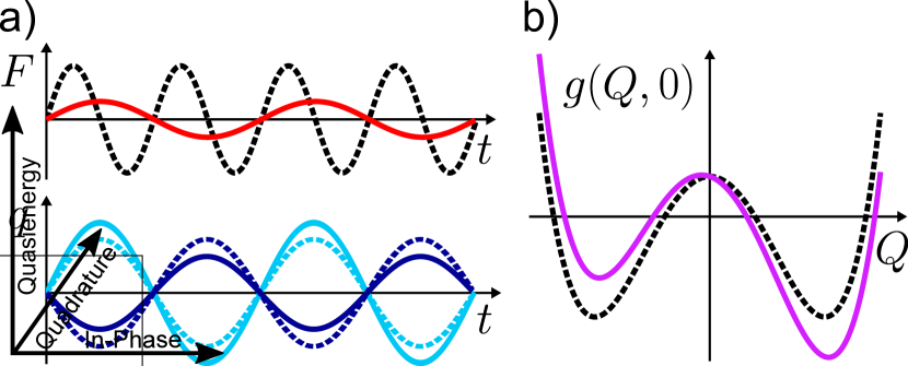
Figure 1: (a) Top panel: sketch of the modulation (dotted line) and the additive extra force (red solid line). Lower panel: Sketch of the vibrating coordinate for the two vibrational states of the oscillator for no extra force (dotted line), the vibrations with the phase close to the phase of the extra force (light blue line), and the vibrations in the counterphase with the force (dark blue line). (b) The cross-section of the scaled Hamiltonian function of the oscillator in the rotating frame $g(Q,P)$ as a function of the quadrature $Q$ for $P=0$. For no extra force $g(Q,P)$ is symmetric, $g(Q,P)=g(-Q,-P)$ (dotted line). The extra force breaks the symmetry, making one well of $g(Q,P)$ deeper and the other well shallower (magenta line).

In the present paper we study the effect of a weak extra drive at frequency $\omega_{p}/2$ on a quantum parametric oscillator. The quantum effect is nonperturbative, in some sense, as it changes the nomenclature of the quantum states. Instead of the Floquet states with the eigenvalues defined modulo $\hbar\omega_{p}$ [20, *Zel'dovich1967, *Ritus1967, *Sambe1973], in the presence of the extra drive the eigenvalues are defined modulo $\hbar\omega_{p}/2$, and even a weak drive can strongly change coherent quantum dynamics. As we show, the drive can have a strong effect in the presence of dissipation, too. We study this effect where the dynamics involves multiple oscillator states, in which case it is exponentially strong. Also, we consider the case where the oscillator eigenfrequency $\omega_{0}$ is close to $\omega_{p}/2$, so that the parametric modulation at frequency $\omega_{p}$ that excites the vibrations can be relatively weak.

Besides the discreteness of the eigenvalue spectrum, a qualitative distinction between the quantum and classical dynamics comes from the nature of the fluctuations associated with the coupling of the oscillator to a thermal bath. Along with classical thermal fluctuations, the coupling leads to quantum fluctuations. In quantum terms, oscillator relaxation comes from transitions between the oscillator states with emission of excitations into the bath. The emission rate determines the relaxation rate, but the very emission events happen at random, leading to noise. In a modulated oscillator, such noise is present even if the bath temperature is $T=0$.

Quantum and classical fluctuations can strongly enhance the effect of the symmetry breaking by a drive at frequency $\omega_{p}/2$. The effect is ultimately determined by the relation between the appropriately scaled drive amplitude and the fluctuation intensity. To provide intuition, we draw an analogy with a Brownian particle in a bistable potential, cf. Fig. 1 (b). Such analogy is seen if one looks at the vibrating oscillator in the frame rotating at $\omega_{p}/2$. Here the dynamics is characterized by the scaled vibration quadratures $Q$ and $P$, i.e., the amplitudes of the vibrational components $\cos(\omega_{p}t/2)$ and $\sin(\omega_{p}t/2)$. These variables can be associated with the scaled coordinate and momentum of the oscillator in the rotating frame.

With no drive at $\omega_{p}/2$, the rotating-frame Hamiltonian is even in $\{Q,P\}$ by symmetry: both $\cos(\omega_{p}t/2)$ and $\sin(\omega_{p}t/2)$ change sign for $t\to t+2\pi/\omega_{p}$, whereas the modulation, and thus the Hamiltonian, do not change. The Hamiltonian becomes time-independent in the rotating wave approximation (RWA). Its cross-section by the plane $P=0$ is sketched in Fig. 1 (b). It has the form of a double-well potential. The minima correspond to the stable vibrational states, in the presence of weak dissipation [24, 25].

A drive at frequency $\omega_{p}/2$ is seen in the rotating frame as a static bias. It breaks the symmetry of the Hamiltonian. The effect is reminiscent of the effect of bias on a Brownian particle in a symmetric double-well potential. With no bias, the potential wells are equally populated. If the bias changes the well depths by $\delta U$, the rates of thermal-noise-induced interwell switching change [26]. As a consequence, the stationary ratio of the well populations changes by $\exp(2\delta U/k_{B}T)$. This factor can be large for small temperature even where $\delta U$ is small compared to the height of the barrier separating the wells.

Similar to a static bias for a Brownian particle, a drive at $\omega_{p}/2$ can exponentially strongly affect the rates of noise-induced switching between the vibrational states of a classical parametric oscillator [27]. As a result, the stationary populations of the states are also strongly changed. The population change was observed for a parametrically modulated mode of a micromechanical resonator by Mahboob et al. [28]. Micromechanical resonators were also used by Han et al. [29] to demonstrate a strong characteristic change of the switching rates.

On the quantum side, of major interest for applications is the regime of comparatively large vibration amplitudes, in which the overlap of the wave functions of the coexisting vibrational states is exponentially small [30]. It corresponds to having many quantum states inside the wells of the scaled RWA Hamiltonian $g(Q,P)$ in Fig. 2. In this case, similar to the classical regime, oscillator relaxation is characterized by two strongly different rates. One is the decay rate in the absence of modulation which, for a modulated oscillator, determines the time it takes to approach a stable vibrational state at one of the minima of $g(Q,P)$. The other is the rate of switching between the stable vibrational states due to classical and quantum fluctuations, which is exponentially smaller for low fluctuation intensity [25].

I.1 Effect of quantum fluctuations on switching between the vibrational states

It is the rate of switching between the vibrational states of a quantum oscillator that can be strongly modified by a weak drive at frequency $\omega_{p}/2$. The effect has generic aspects, which go beyond the model of the parametric oscillator. They manifest most clearly where the decay rate is small, so that the spacing of the intrawell levels of the RWA Hamiltonian significantly exceeds their width. In this regime, a major effect of the coupling to a thermal bath is transitions between the RWA states, see Fig. 2. The transitions are not limited to the neighbouring RWA states even where the relaxation is due to transitions between the neighboring Fock states. Transitions down to the bottom of the well of the RWA Hamiltonian are more likely then toward the barrier top, the rates $W_{\downarrow}$ are larger than $W_{\uparrow}$. Therefore the oscillator is mostly localized near one or the other minimum of the well . However, since $W_{\uparrow}$ is nonzero, the oscillator essentially performs a random walk over the intrawell states. In the course of this walk it can reach the barrier top and then switch to the other well with probability $\sim 1/2$.

We note the difference between the rates of transitions between the quantum intrawell states sketched in Fig. 2 and the rate of switching between the stable vibrational states. We use the term “switching” to describe transitions between the wells of the RWA Hamiltonian.

A remarkable feature of the dynamics in the absence of an extra drive is the fragility of the low-temperature behavior. If the oscillator Planck number $\bar{n}=[\exp(\hbar\omega_{p}/2k_{B}T)-1]^{-1}$ can be set equal to zero, the rates of transitions between the intrawell states meet the conventional relation [32] of systems with detailed balance [25]. For systems in thermal equilibrium it follows from the time-reversal symmetry and can be traced back to Einstein [33]. For a parametric oscillator, the transition rates, and ultimately the rate of interwell switching, are determined by purely quantum fluctuations.

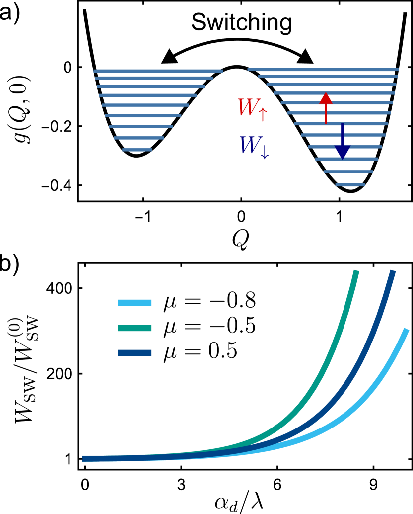
Figure 2: (a) Scaled quasienergy levels of the oscillator for the parameters $\mu=0.2$, $\lambda=\alpha/2=0.02$, and $\varphi=\pi/2$, see Eqs. (II) - (6). $W_{\uparrow}$ and $W_{\downarrow}$ indicate transitions due to the coupling to a thermal bath; the transitions are not limited to the nearest quasienergy levels. The rate of transitions down is higher than the rate of transitions up. The states at the bottom of the wells of $g(Q,0)$ correspond to the stable vibrational states. (b) The strong change of the switching rate with the varying scaled amplitude of the extra force $\alpha_{d}$ divided by the scaled Planck constant $\lambda$ for three values of the scaled difference $\mu$ between the oscillator eigenfrequency and half the modulation frequency.

The thermal contribution to the rates of intrawell transitions, which is $\propto\bar{n}$, does not meet the detailed balance condition. Moreover, even where $\bar{n}$ is still extremely small, the exponent of the rate of interwell switching can change. The change is almost discontinuous with respect to $\bar{n}$ [25]. This is because the rates $W_{\uparrow}$ of thermally induced intrawell transitions fall off with the distance between the intrawell states exponentially slower than the $\bar{n}=0$-rates, making it much easier to reach the barrier top in the random walk over the intrawell states.

In this paper we address the question of whether a weak extra drive can break the fragility of the detailed-balance relation between the transition rates for $\bar{n}=0$. Besides the importance of understanding it, the effect has an interesting general aspect, as we now explain.

The RWA-dynamics of a parametric oscillator can be described by a diffusion equation for the Glauber-Sudarshan $P(\alpha,\alpha^{*})$-function, where $\ket{\alpha}$ is a coherent state [1, 4, 10, 12]. For $\bar{n}=0$ this equation meets the so-called “potential condition” [34]: the probability current in the $\alpha$-variables is zero in the stationary regime. Vanishing of the current in the diffusion equation is often associated with detailed balance. For a parametric oscillator, it happens both without [1] and with [4, 12] an extra drive at $\omega_{p}/2$.

As we will show, a drive at $\omega_{p}/2$ breaks the detailed-balance relation between the intrawell transition rates. This changes the rates of interwell switching very strongly, in a sense, anomalously strongly. However, as indicated above, the probability current in the $\alpha$-variables is still zero in the stationary regime. The result should be compared with the effect of the terms $\propto\bar{n}$ in the intrawell transition rates, which lead to a nonzero probability current in the stationary solution of the diffusion equation for $P(\alpha,\alpha^{*})$. The unexpected effect of the extra drive shows that care must be taken when associating zero probability current in the diffusion equation with the presence of detailed balance.

I.2 The outline of the paper

To set the scene, in Sec. II we introduce the Hamiltonian of the parametrically modulated nonlinear oscillator. We show that the Hamiltonian has two wells and discuss the intrawell dynamics in the presence of a weak drive. In Sec. III we present the master equation, which describes the effect of the coupling to a thermal bath on the oscillator dynamics. We reduce this equation to the balance equation for the populations of the intrawell states in the weak-damping limit. We explain how this balance equation can be solved within the WKB approximation and how the interwell switching rates are found from this solution. Section IV is technical: we use the methods of nonlinear dynamics to develop a perturbation theory that allows us to find corrections to the transition rates, which are linear in the amplitude of the extra drive. The result is used in Sec. V to find the corrections to the intrawell state populations and to the switching rate for not too small $\bar{n}$. The change of the logarithm of the switching rate is linear in the extra drive amplitude. We find the corresponding logarithmic susceptibility and its dependence on $\bar{n}$ and the oscillator parameters. The explicit expressions are obtained for comparatively high temperatures and close to the bifurcation point where there emerge period-2 vibrations; in particular, we consider the prebifurcation scaling where the motion near the bifurcation point is still underdamped. In Sec. VI we show that the perturbation theory in the amplitude of the extra drive breaks down for $\bar{n}=0$ in the semiclassical limit. We find the distribution over the intrawell states. In Sec.  VII we use the result to find the switching rates and the stationary distribution over the vibrational states of the oscillator. Section VIII contains concluding remarks.

II THE HAMILTONIAN IN THE ROTATING WAVE APPROXIMATION

If the decay rate of the oscillator $\Gamma$ is small compared to its eigenfrequency $\omega_{0}$, even a comparatively small periodic modulation of $\omega_{0}$ at frequency $\omega_{p}$ close to $2\omega_{0}$ can lead to bistability. The onset of stable states requires that the oscillator be nonlinear [35]. Classically, the vibration frequency of a nonlinear oscillator depends on its amplitude. Therefore, as the amplitude of the parametrically excited vibrations increases, the vibration frequency moves away from $\omega_{p}/2$, weakening the resonance with the modulation and stabilizing the vibrations.

A simple nonlinearity of the oscillator potential that leads to the stabilization in the lowest order of the perturbation theory is the Duffing (Kerr) nonlinearity. It is relevant to many physical systems and is described by the quartic term in the oscillator coordinate $q_{0}$. The Hamiltonian of the parametrically modulated Duffing oscillator has the form

$$H^{(0)} =\frac{1}{2}p_{0}^{2}+\frac{1}{2}q_{0}^{2}\left[\omega_{0}^{2}+F_{p}\cos(\omega_{p}t)\right]+\frac{1}{4}\gamma q_{0}^{4},$$ (1)

where $q_{0}$ and $p_{0}$ are the oscillator coordinate and momentum, $F_{p}$ is the modulation amplitude, $\gamma$ is the nonlinearity parameter, and we have set the oscillator mass equal to unity.

In the presence of an additional linear drive at half the modulation frequency the Hamiltonian becomes

$$H=H^{(0)}-q_{0}A_{d}\cos(\omega_{p}t/2+\varphi_{d}),$$ (2)

where $A_{d}$ and $\varphi_{d}$ are the amplitude and phase of the drive.

The oscillator dynamics is conveniently described by switching to the rotating frame with the unitary transformation $\hat{U}=\exp[-i\hat{a}^{\dagger}\hat{a}(\omega_{p}t/2)]$, where $\hat{a}^{\dagger}$ and $\hat{a}$ are the ladder operators, $\hat{a}=(\hbar\omega_{p})^{-1/2}(i\hat{p}_{0}+\omega_{p}\hat{q}_{0}/2)$. In the rotating wave approximation (RWA) the von Neumann equation for the oscillator density matrix $\hat{\rho}$ in the rotating frame reads

$$d\hat{\rho}/d\tau=i\lambda^{-1}[\hat{\rho},\hat{g}],\qquad\tau=tF/2\omega_{p}.$$ (3)

Here $\hat{g}$ is the scaled RWA Hamiltonian,

$$\hat{g}\equiv\hat{g}(Q,P)=\hat{g}^{(0)}+\alpha_{d}\hat{g}^{(1)},$$

$$\hat{g}^{(0)}=\frac{1}{4}(Q^{2}+P^{2})^{2}+\frac{1}{2}(1-\mu)P^{2}-\frac{1}{2}(1+\mu)Q^{2}\,,$$

$$\hat{g}^{(1)}=-\left[P\cos\varphi_{d}+Q\sin\varphi_{d}\right].$$ (4)

In Eqs. (3) and (II) $Q$ and $P$ are the dimensionless coordinate and momentum, $\tau=tF/2\omega_{p}$ is the dimensionless time, and $\alpha_{d}=A_{d}\sqrt{6\gamma/F_{p}^{3}}$ is the scaled amplitude of the extra additive drive. Here and in what follows we use the superscripts $0$ and $1$ to indicate the parameters of the oscillator unperturbed by the extra drive and the perturbation, respectively. For a weak extra drive that we consider $\alpha_{d}\ll 1$.

In terms of the ladder operators in the rotating frame

$$\hat{Q}= i(\lambda/2)^{1/2}(\hat{a}-\hat{a}^{\dagger}),\quad\hat{P}=(\lambda/2)^{1/2}(\hat{a}+\hat{a}^{\dagger}),$$

$$\hat{g}= \lambda^{2}(\hat{a}^{\dagger}\hat{a}+1/2)^{2}+\frac{\lambda}{2}(\hat{a}^{2}+\hat{a}^{\dagger^{2}})-\mu\lambda\hat{a}^{\dagger}\hat{a}$$

$$-\alpha_{d}\sqrt{\frac{\lambda}{2}}\left(\hat{a}e^{i\varphi_{d}}+\mathrm{c.c.}\right)\,,$$ (5)

where $\lambda=3\gamma\hbar/F_{p}\omega_{p}$ is the scaled Planck constant, $[\hat{Q},\hat{P}]=i\lambda$. In the absence of the extra drive the Hamiltonian $\hat{g}(Q,P)$ depends only on one parameter, the scaled detuning

$$\mu=2\omega_{p}\delta\omega/F_{p},\qquad\delta\omega=\omega_{p}/2-\omega_{0}.$$ (6)

We note that, since we switched to the rotating frame at half the modulation frequency, in the absence of extra additive drive $\propto A_{d}$ the Hamiltonian $\hat{g}^{(0)}(Q,P)$ is not the Floquet (quasienergy) Hamiltonian. To avoid confusion we call $g$ the RWA Hamiltonian, and its eigenvalues the RWA energy values.

II.1 Intrawell dynamics

The unperturbed RWA Hamiltonian $\hat{g}^{(0)}(Q,P)$ is a symmetric function of $Q$ and $P$. For $-1<\mu<1$ it has two minima. They lie on the $Q$-axis at ${Q^{(0)}_{\pm}=\pm\sqrt{1+\mu}}$. At the minima ${g^{(0)}(Q^{(0)}_{\pm},P=0)\equiv g_{\mathrm{min}}^{(0)}=-(1+\mu)^{2}/4}$. In the laboratory frame, the minima correspond to parametrically excited vibrations with opposite phases; the coordinate $q_{0}(t)$ is $\propto-Q_{\pm}^{(0)}\sin(\omega_{p}t/2)$.

The minima are separated by a saddle point at $Q=P=0$. Classical Hamiltonian dynamics inside the symmetric wells of the function $g^{(0)}(Q,P)$ is well understood [25]. The oscillator moves along closed intrawell trajectories with constant RWA-energy, $g^{(0)}(Q,P)=g$. The trajectories in the opposite wells are mirror-symmetric and, for a given $g$, have the same frequency $\omega^{(0)}(g)$.

We now consider the effect of the drive $\propto\alpha_{d}$ on the classical trajectories inside the wells. The drive breaks the symmetry of $g(Q,P)$, as it tilts it. The direction of the tilt is determined by the phase $\varphi_{d}$. For a weak drive, $\alpha_{d}\ll 1$, the function $g(Q,P)$ still has two wells, which are now asymmetric and may have different depths. For the phase $\varphi_{d}=(2k+1)\pi/2$ with integer $k$ the tilt is along the $Q$ axis. The minimum of one well shifts towards the origin and the well depth decreases, while the other well shifts away from the origin and its depth increases. For $\varphi_{d}=k\pi$ the wells are shifted along the $P$ axis. In the general case, to the first order in $\alpha_{d}$ the values of $g(Q,P)$ at the minima are

$$g_{\mathrm{min}{}}=g_{\mathrm{min}}^{(0)}\pm\alpha_{d}g_{\mathrm{min}}^{(1)}\,,\quad g_{\mathrm{min}}^{(1)}=-\sqrt{1+\mu}\sin\varphi_{d}\,.$$ (7)

where the signs “$+$” and “$-$” refer to the wells at $Q>0$ and $Q<0$, respectively. The saddle point of $g(Q,P)$ shifts from $Q=P=0$ to $Q=-\alpha_{d}\sin\varphi_{d}/(1+\mu)$ and $P=-\alpha_{d}\cos\varphi_{d}/(1-\mu)$. The value $g_{\mathrm{saddle}}$ of $g(Q,P)$ at the saddle point does not change, to the first order in $\alpha_{d}$.

The change of $g(Q,P)$ due to the drive $\propto\alpha_{d}$ leads to a change of the Hamiltonian intrawell trajectories. Generally, we expect the frequency $\omega(g)$ to change, too. The frequency can be found by calculating the action variable $I_{f}$ as a function of the RWA energy $g$,

$$\omega^{-1}(g)=\partialderivative{I_{f}(g)}{g}\,,\qquad I_{f}(g)=\frac{1}{2\pi}\oint P(Q|g)d{}{}{Q}\,,$$

where the integral is taken over the trajectory with a given $g$ inside the well; $P(Q|g)$ is given by the equation $g(Q,P)=g$. We use the subscript $f$ to indicate that $I_{f}$ refers to the full Hamiltonian function $g=g^{(0)}+\alpha_{d}g^{(1)}$. In Appendix A we show that, to the first order in $\alpha_{d}$, the actions in the two wells change by $\pm\alpha_{d}I_{f}^{(1)}=\pm\alpha_{d}\sin(\varphi_{d})/2$. Remarkably this change is independent of $g$, see Fig. 3 (b). Then, to the first order in $\alpha_{d}$, the frequency of intrawell classical motion is not changed by the linear drive. This has interesting consequences for the energy spectrum of the RWA Hamiltonian.

Figure 3: (a) Classical Hamiltonian trajectories $g=~{}$const. inside the well of the RWA Hamiltonian $g(Q,P)$ at $Q>0$ for $g=-0.6$. (b) The dependence of the action variable on the RWA energy $g$. Both panels refer to $\mu=0.7$ and $\varphi_{d}=\pi/6$.

II.2 The RWA energy levels

For the dimensionless RWA Hamiltonian $\hat{g}$, the distance between the eigenvalues, i.e., between the RWA energy levels, is proportional to the dimensionless effective Planck constant $\lambda$. As indicated earlier, of interest for quantum information and for many other physics problems is the case where there are many quantum states $\ket{n}$ inside the wells of the function $g(Q,P)$. This implies that $\lambda\ll 1$. Moreover, we will be interested in the regime where the extra drive, although weak, is still “quantum strong”, that is the drive-induced shift of the RWA energy levels is larger than the level spacing, which implies that $\lambda\ll\alpha_{d}$. Respectively, the shift of the minima $|\alpha_{d}g_{\min}^{(1)}|$ significantly exceeds the spacing of the levels as well.

Since for $\alpha_{d}=0$ the wells of $g(Q,P)$ are symmetric and intrawell states of different wells are in resonance, the eigenstates of $\hat{g}$ are given by the tunnel split symmetric and antisymmetric combinations of the intrawell states. As $\alpha_{d}$ increases, the levels in different wells shift away from each other and resonant tunneling is suppressed. The eigenstates $\ket{n}$ of $\hat{g}$ are well-localized intrawell states,

$$\hat{g}\ket{n}=g_{n}\ket{n}.$$

where $g_{n}$ are the intawell RWA energies.

We note that a part of the states in different wells may become resonant again for certain values of $\alpha_{d}$. In the semiclassical limit, the distance between the intrawell levels $g_{n}$ is $\lambda\omega(g)$. Therefore, given that $\omega(g)$ is not changed by the drive, for such $\alpha_{d}$, simultaneously, all levels in the shallow well come to resonance with the levels in the deeper well.

III QUANTUM ACTIVATION

Coupling the oscillator to a thermal bath leads to dissipation. In the absence of modulation, dissipation is associated with transitions between the Fock states of the oscillator (i.e., the eigenstates of the Hamiltonian $H^{(0)}$ for $F_{p}=0$), which are accompanied by emission and absorption of excitations of the bath. A major dissipation process is associated with transitions between neighbouring Fock states, with energy exchange $\approx\hbar\omega_{0}$. Classically, it leads to a viscous-type friction force $2\Gamma\dot{q}_{0}$. We will assume that the coupling is weak, so that the friction coefficient $\Gamma$ is small compared to the oscillator eigenfrequency $\omega_{0}$. If certain well-understood conditions are met, the oscillator dynamics is Markovian on the time scale slow compared to $\omega_{0}^{-1}$ [36].

Resonant parametric modulation does not open new dissipation channels, to the leading order in $F_{p}$. However, now the state nomenclature is changed: dissipative transitions between the Fock states of the oscillator translate to transitions between the RWA states, since the latter states are linear combinations of the former states. Because the overlapping of the RWA states in different wells is exponentially small for small $\lambda$, of primary importance are transitions between the states within the same well. It is characteristic that the transitions between neighboring Fock states are projected onto transitions between not only neighbouring, but also remote RWA states. In the absence of an extra drive, the rates $W_{nn^{\prime}}$ of transitions between intrawell states $\ket{n}\to\ket{n^{\prime}}$ were calculated earlier [25].

If the rates $W_{nn^{\prime}}$ are small compared to the levels spacing $\lambda\omega(g)$, the dynamics of the parametric oscillator can be described by the balance equation for the intrawell state populations $\rho_{n}=\bra{n}\rho\ket{n}$,

$$\partialderivative{\rho_{n}}{\tau} =-\sum_{n^{\prime}}(W_{nn^{\prime}}\rho_{n}-W_{n^{\prime}n}\rho_{n^{\prime}})\,,$$

$$W_{nn^{\prime}} =W_{nn^{\prime}}^{\mathrm{(e)}}+W_{nn^{\prime}}^{\mathrm{(abs)}}\,,\quad W_{nn^{\prime}}^{\mathrm{(abs)}}=2\kappa\bar{n}\absolutevalue{\Braket{n}{\hat{a}}{n^{\prime}}}^{2}\,,$$

$$W_{nn^{\prime}}^{\mathrm{(e)}} =2\kappa(\bar{n}+1)\absolutevalue{\Braket{n}{\hat{a}^{\dagger}}{n^{\prime}}}^{2}\,.$$ (8)

Here, $\bar{n}=[\exp{\hbar\omega_{p}/2k_{B}T}-1]^{-1}$ is the oscillator thermal occupation number; $\kappa$ is the scaled friction coefficient, $\kappa=2\Gamma\omega_{p}/F_{p}$. We omitted the indices that label the wells.

In the semiclassical approximation, where $n,n^{\prime}\gg 1$ and $|n-n^{\prime}|$ is not too large, we can express the matrix elements in Eq. (III) by the Fourier transforms of the complex amplitudes of intrawell vibrations [17],

$$\braket{n+m}{\hat{a}}{n}\approx a_{m}(g_{n}),$$

$$a_{m}(g)=\frac{1}{2\pi}\int_{0}^{2\pi}d{}{}\phi\,a(\tau,g)e^{-im\phi}\,,$$ (9)

where $\phi=\omega(g)\tau$ and $a(\tau,g)=(2\lambda)^{-1/2}[P(\tau,g)-iQ(\tau,g)]$; $Q(\tau,g)$ and $P(\tau,g)$ are the solution of the Hamiltonian equations of motion for the Hamiltonian in Eq. (II). The expressions for the transition rates in terms of $a_{m}(g)$ have the form

$$W_{n+m\,n}^{\mathrm{(e)}} =2\kappa(\bar{n}+1)\absolutevalue{a_{-m}(g_{n})}^{2}\,,$$

$$W_{n+m\,n}^{\mathrm{(abs)}} =2\kappa\bar{n}\absolutevalue{a_{m}(g_{n})}^{2}\,.$$ (10)

An explicit calculation of the matrix elements $\braket{n}{\hat{a}}{n^{\prime}}$ shows [25] that, in the absence of the extra drive, the transition rates $W_{nn^{\prime}}$ satisfy the condition $W_{nn^{\prime}}>W_{n^{\prime}n}$ for $n>n^{\prime}$, if we use the convention that the states $\ket{n}$ are counted off from the bottom of the well of $g(Q,P)$. This strong inequality cannot be broken by a weak extra drive. It means that the oscillator is more likely to go down towards the bottom of the well than going up away from it. This corresponds to relaxation to a classically stable state, in quantum terms.

The transition probabilities have two contributions corresponding to absorption and emission of excitations of the heat bath. Importantly, even in the regime where the thermal occupation number $\bar{n}$ can be assumed to be zero and only emission processes are relevant, transitions away from the bottom of the well still have nonzero probability, populating excited intrawell states. This effect was termed quantum heating [37] and was directly observed in the experiment [38]. In the random walk over intrawell states, once the oscillator makes a transition away from the bottom of the well, it is more likely to go back down, but it still can go further up. Ultimately, if it reaches the top of the well, where $g(Q,P)=0$, it can switch to another well. Such switching is similar to thermal activation in equilibrium systems and has been called quantum activation. In what follows, since $\bar{n}$ depends on temperature exponentially for $k_{B}T\ll\hbar\omega_{p}$, we use the term “zero temperature” for the regime where we set $W_{nn^{\prime}}^{\mathrm{abs}}=0$.

III.1 Discrete WKB approximation

In order to calculate the rate $W_{\mathrm{sw}}$ of interwell switching we investigate the quasistationary distribution over intrawell states described by Eq. (III) in which we set $\partial\rho_{n}/\partial\tau=0$. Such approach is justified by the strong inequality $W_{\mathrm{sw}}\ll\kappa$ and is similar to the analysis of the switching rate in thermal equilibrium systems [26]. To find the quasistationary distribution in the semiclassical range, where the number of intrawell states is large, we use the Ansatz

$$\rho_{n}=\exp[-R(g_{n})/\lambda]$$ (11)

and use that (i) $R(g)$ is a smooth function of $g$ and that (ii) $W_{n+m\,n}\approx W_{n\,n-m}$. The latter condition is based on the fact that the rates $W_{n\,n+m}$ fall off exponentially with the increasing $|m|$ and that the typical $n$ are much larger than the typical $|m|$. Then Eq. (III) is reduced to a set of linear equations for $R^{\prime}(g)$,

$$\sum_{m}W_{n+m\,n}(1-\xi_{n}^{m})=0\,,$$ (12)

$$\xi_{n}=\exp[-\omega(g_{n})R^{\prime}(g_{n})]\,,\qquad R^{\prime}(g)=dR(g)/dg\,,$$

where we used $g_{n+m}-g_{n}\approx m\lambda\omega(g_{n})$. The quasistationary distribution (11) inside a well is determined by the function

$$R(g) =\int_{g_{\mathrm{min}}}^{g}R^{\prime}(x)\,dx\,.$$

The rate of switching from a well $W_{\mathrm{sw}}$ is approximately given by the probability per unit time to reach a state with $g$ close to the saddle-point energy $g_{\mathrm{saddle}}$

$$W_{\mathrm{sw}} =C_{\mathrm{sw}}\times\exp(-R_{\mathrm{A}}/\lambda)\,,\quad R_{\mathrm{A}}=R(g_{\mathrm{saddle}})$$ (13)

To the first order in the amplitude of the extra drive, $g_{\mathrm{saddle}}=0$. The prefactor $C_{\mathrm{sw}}$ in Eq. (13) is proportional to the decay rate in the absence of modulation $\kappa$.

IV Effect of the extra drive on the transition rates

We emphasize again that we consider the dynamics in one of the wells of $g(Q,P)$. The extra drive not only shifts the RWA energies of the intrawell states, but also modifies the transitions rates $W_{n\,n\pm m}$ by changing the matrix elements $a_{m}(g_{n})=\braket{n+m}{\hat{a}}{n}$. We calculate the corrections to $a_{m}(g)$ in Eq. (III) assuming that the perturbation is classically weak, $\alpha_{d}\ll 1$.

Where there is no extra drive, the classical trajectories $Q(\tau,g),P(\tau,g)$ can be expressed in terms of the Jacobi elliptic functions, leading to simple expressions for their Fourier components [25], see Appendix A. The drive changes the trajectories, and we have not found analytical expressions for them. Examples of the trajectories with and without a weak extra drive are shown in Fig. 3 (a).

IV.1 Action-angle variables

It is convenient to find the drive-induced corrections to $a_{m}(g)$ by switching to the action-angle variables $I,\psi$ of the unperturbed system. Formally, we proceed by considering a system with the coordinate $q$, momentum $p$, and the Hamiltonian function $g^{(0)}(q,p)$ and make a standard canonical transformation

$$p=\partial S(q,I)/\partial q,\quad\psi=\partial S(q,I)/\partial I,$$

$$I(g)=\frac{1}{2\pi}\oint p(q|g)dq\,,\quad g^{(0)}(q,p)=g,$$

$$q(I;\psi+2\pi)=q(I;\psi),\quad p(I;\psi+2\pi)=p(I;\psi),$$ (14)

where the generating function $S$ is the action calculated for the unperturbed Hamiltonian $g^{(0)}$ and $p(q|g)$ is the momentum calculated from the equation $g^{(0)}(q,p)=g$. The explicit relation between $(q,p)$ and $(I,\psi)$ can be found from the Fourier components of $q,p$ calculated for the Hamiltonian $g^{(0)}$, see Appendix A. The function $I(g)$ satisfies the equation

$$d{}I/d{}g=1/\omega^{(0)}(g),\quad g=g^{(0)}\bigl{(}q(I;\psi),p(I;\psi)\bigr{)}=g^{(0)}(I),$$

where $\omega^{(0)}(g)$ is the frequency of intrawell vibrations in the absence of extra drive; it is given in Appendix A. The above equation gives the Hamiltonian function $g^{(0)}$ as a function of the action, $g^{(0)}(I;\psi)\equiv g^{(0)}(I)$.

In what follows we will consider the coordinate and momentum of the oscillator $Q,P$ in the presence of the extra drive as functions of $I,\psi$. We define their functional form as

$$Q(I;\psi)=q(I;\psi),\quad P(I,\psi)=p(I;\psi);$$

$$g^{(0)}(Q,P)=g^{(0)}(I).$$

We distinguish between the functions $Q(\tau,g)$ and $Q(I;\psi)$ by making use of the semicolon. The same convention is used for $P(I;\psi)$.

The full RWA Hamiltonian is time-independent. However, since $I$ and $\psi$ are defined with respect to $g^{(0)}$, in the presence of the extra drive the action $I$ depends on time and the time dependence of $\psi$ is changed compared to the case where there is no extra drive. To find the time dependence of $I,\psi$ one has to express the Hamiltonian function $g=g^{(0)}+\alpha_{d}g^{(1)}$ in terms of $I,\psi$. To emphasize this form of the Hamiltonian we write it as $G(I;\psi)=G^{(0)}(I;\psi)+\alpha_{d}G^{(1)}(I;\psi)$, where

$$G^{(\alpha)}(I;\psi)=g^{(\alpha)}\bigl{(}Q(I;\psi),P(I;\psi)\bigr{)},\quad\alpha=0,1.$$

Since $G^{(0)}$ and $G^{(1)}$ are obtained from Eq. (II) by substituting $Q=Q(I;\psi),\,P=P(I;\psi)$, they are periodic in $\psi$. The equations of motion for $I,\psi$ read

$$\frac{dI}{d\tau}=-\partialderivative{G}{\psi}\,,\qquad\frac{d\psi}{d\tau}=\partialderivative{G}{I}\,,$$

$$G\equiv G(I;\psi)=G^{(0)}+\alpha_{d}G^{(1)}=G(I;\psi+2\pi)\,.$$ (15)

These are Hamiltonian equations describing trajectories with a constant RWA energy $G(I;\psi)=g$. By construction

$$G^{(0)}(I;\psi)=\int_{0}^{I}dI^{\prime}\,\Omega^{(0)}(I^{\prime})+g_{\mathrm{min}}^{(0)}\,.$$

$$\Omega^{(0)}(I)\equiv\omega^{(0)}\bigl{(}g^{(0)}(I)\bigr{)}$$ (16)

The frequency $\Omega^{(0)}(I)$ is the vibration frequency for the unperturbed system as a function of the action $I$.

To find the extra-drive induced corrections to the Fourier components $a_{m}(g)$, we will seek corrections to $I$ and $\psi$ for a given RWA energy $g=G^{(0)}+\alpha_{d}G^{(1)}$. Because ultimately we need corrections to the Fourier components of the variables $Q,P$, the analysis is slightly different from the conventional analysis of nonlinear dynamics [39].

From Eq. (IV.1), to the first order in $\alpha_{d}$

$$I(\tau) =I^{(0)}+\alpha_{d}I^{(1)}(\tau),$$

$$\psi(\tau) =\Omega^{(0)}(\bar{I})\tau+\alpha_{d}\psi^{(1)}(\tau)\,.$$ (17)

Here and in what follows the overline means period averaging. Both $I^{(1)}$ and $\psi^{(1)}$ are periodic functions of time, as they are determined by $G^{(1)}$. In particular, $\psi^{(1)}(\tau)$ comes from integrating over time the term $\partial G^{(1)}/\partial I$ in Eq. (IV.1) for $d\psi/d\tau$, but this is not the only first-order correction to $\psi(\tau)$, as explained below.

IV.2 Vibration frequency for a given intrawell energy

The vibration frequency inside a well of $g(Q,P)$ is determined by the secular term $\propto\tau$ in $\psi(\tau)$. There are two extra-drive induced contributions to this term. One comes from the difference between $\bar{I}$ and $I^{(0)}$ in the term $\propto\Omega^{(0)}(\bar{I})$ in Eq, (IV.1). To the first order in $\alpha_{d}$, the value of $\bar{I}$ for a given $g$ has to be found from the equation $G^{(0)}(\bar{I})+\alpha_{d}\bar{G}^{(1)}=g$. From this equation we find $\bar{I}=I^{(0)}+\alpha_{d}\bar{I}^{(1)}$ with $\bar{I}^{(1)}=-\bar{G}^{(1)}/\Omega^{(0)}$ (both $\bar{G}^{(1)}$ and $\Omega^{(0)}$ here are calculated for $I=I^{(0)}$).

The second secular contribution is contained in $\psi^{(1)}(\tau)$ and comes from the term $\partial\bar{G}^{(1)}/\partial I$ in Eq. (IV.1) for $d\psi/d\tau$. From Eqs. (A.1) and (50), $\bar{G}^{(1)}=\bar{C}\Omega^{(0)}(I^{(0)})$, where $\bar{C}$ is independent of $I$. Therefore the secular term in $\psi^{(1)}$ cancels the secular correction $\propto\bar{I}^{(1)}$ in $\psi(\tau)$. Indeed, $(d\Omega^{(0)}/dI)\bar{I}^{(1)}+(d\bar{G}^{(1)}/dI)=0$. As a result, to the first order in $\alpha_{d}$, the secular term in $\psi(\tau)$ is $\omega^{(0)}(g)\tau$, and therefore the oscillating terms are $\propto\exp(in\omega^{(0)}(g)\tau)$ with integer $|n|>0$,

$$\psi(\tau)=\omega^{(0)}(g)\tau+\alpha_{d}\sum_{n\neq 0}\psi_{n}^{(1)}\exp[in\omega^{(0)}(g)\tau]\,,$$ (18)

where $\psi_{n}^{(1)}\equiv\psi_{n}^{(1)}(g)$ are the Fourier components of $\psi^{(1)}$. To the same order of the perturbation theory, $I^{(1)}(\tau)$ is a sum of terms $\propto\exp[in\omega^{(0)}(g)\tau]$ with $n\neq 0$. They, as well as $\psi_{n}^{(1)}$, are immediately expressed in terms of the Fourier components of $G^{(1)}$, see Appendix B.

We can now calculate the corrections to the Fourier components $a_{m}(g)$ to the first order in $\alpha_{d}$. We write

$$a(\tau,g)\equiv a(I;\psi)=[P(I;\psi)-iQ(I;\psi)]/\sqrt{2\lambda}.$$

The functions $Q(I;\psi)$ and $P(I;\psi)$ are periodic functions of $\psi$, while $I\equiv I(\tau)$ and $\psi\equiv\psi(\tau)$ are periodic functions of time with frequency $\omega^{(0)}(g)$. The Fourier components

$$a_{m}(g)=\frac{1}{2\pi}\int_{0}^{2\pi}d\phi\,a(\tau,g)\exp(-im\phi)$$

with $\phi=\omega^{(0)}(g)\tau$ are determined by the Fourier components of $a(I;\psi)$. To find $a_{m}(g)$ we expand $a(I;\psi)$ to the first order in $I^{(1)},\psi^{(1)}$, and use the Fourier series for $I^{(1)},\psi^{(1)}$, cf. Eq. (18). This gives

$$a_{m}(g)\approx a_{m}^{(0)}(g)+\alpha_{d}a_{m}^{(1)}(g)\,,$$

$$a_{m}^{(1)}=\sum_{k}\left[J_{mk}a_{m-k}^{(0)}+L_{mk}(d{}a_{m-k}^{(0)}/d{}g)\right]\,.$$ (19)

Explicit expressions for the parameters $J_{mk}\equiv J_{mk}(g)$ and $L_{mk}\equiv L_{mk}(g)$ follow from Eq.(B) in Appendix B. They apply in the range $g>\max\{g_{\mathrm{min}},g_{\mathrm{min}}^{(0)}\}$. It is straightforward also to find higher-order corrections to $I,\psi$ and then to $a(I;\psi)$. We note that the vibration frequency will be shifted from $\omega^{(0)}(g)$ in the second order in $\alpha_{d}$.

IV.3 Transition rates to the first order in $\alpha_{d}$

Corrections to the emission and absorption transition rates $W_{nn^{\prime}}^{\mathrm{(e)}}$ and $W_{nn^{\prime}}^{\mathrm{(abs)}}$ are found by inserting the expansion for $a_{m}(g_{n})$ into Eq. (III). This gives the rates in the form of perturbation series

$$W_{n+m\,n}=W_{n+m\,n}^{(0)}+\alpha_{d}W_{n+m\,n}^{(1)}+\alpha_{d}^{2}W_{n+m\,n}^{(2)}+\ldots\,,$$

$$(W_{n+m\,n}^{\mathrm{(e)}})^{(1)}=4\kappa(\bar{n}+1)\,\mathrm{Re}\,\left[a_{-m}^{(0)}{}^{*}(g_{n})a_{-m}^{(1)}(g_{n})\right]$$

$$(W_{n+m\,n}^{\mathrm{(abs)}})^{(1)}=4\kappa\bar{n}\,\mathrm{Re}\,\left[a_{m}^{(0)}{}^{*}(g_{n})a_{m}^{(1)}(g_{n})\right]$$ (20)

In turn, this allows finding corrections to the populations of the intrawell states $\rho_{n}$ and the rate $W_{\mathrm{sw}}$ of interwell switching. The term $W_{n+m\,n}^{(2)}$ in Eq. (IV.3) is $\propto\alpha_{d}^{2}$; it is discussed in Sec. VI.

An important feature of the rates $W^{(1)}$ is their specific dependence on the phase of the extra drive. We find that $W^{(1)}_{n+m\,n}\propto\sin\varphi_{d}$. This is in spite of $a_{m}^{(1)}(g)$ being a linear combination of $\cos\varphi_{d}$ and $\sin\varphi_{d}$. Formally, this is a consequence of $a_{m}^{(0)}$ being purely imaginary, see Eq. (A), whereas the term $\propto\cos\varphi_{d}$ in $a_{m}^{(1)}$ is real, as shown in Appendix B, see also Appendix C, and drops out from $\mathrm{Re}\,[(a_{m}^{(0)})^{*}\,a_{m}^{(1)}]$. We note that the fact that $\cos\varphi_{d}$ does not affect the quantum dynamics is a consequence of the approximation of slow relaxation, where the dynamics is described by the balance equation for the state populations (III).

V LOGARITHMIC SUSCEPTIBILITY FOR NOT TOO SMALL $\bar{n}$

The number of intrawell states of the oscillator is $\sim 1/\lambda\gg 1$. Therefore corrections to the rates of interstate transitions accumulate to exponentially large changes of the populations of highly excited states and to a change of the quantum activation energy $R_{\mathrm{A}}$ of the interwell switching. In particular, $R_{\mathrm{A}}$ acquires a linear in $\alpha_{d}$ correction, so that the switching rate $W_{\mathrm{sw}}\propto\exp(-R_{\mathrm{A}}/\lambda)$ changes exponentially strongly for $\alpha_{d}\gg\lambda$ even where the drive is weak, $\alpha_{d}\ll 1$. The factor multiplying $A_{d}\propto\alpha_{d}$ in the expression for $R_{\mathrm{A}}\propto\lambda|\log W_{\mathrm{sw}}|$ is the logarithmic susceptibility (more generally, the logarithmic susceptibility depends on the drive frequency [40, 27]).

In the absence of an extra drive the oscillator displays qualitatively different dynamics depending on the thermal occupation number $\bar{n}$ [25]. For $\bar{n}=0$ the rates of transitions between the states are determined by emission of excitations of the medium, $W_{n+m\,n}=W_{n+m\,n}^{\mathrm{(e)}}$, and the oscillator has detailed balance, as we discuss in more detail in Sec. VI. In contrast, interstate transitions due to absorption of excitations of the medium, whose rates are $\propto\bar{n}$, break the detailed balance. Concurrently, beyond a narrow range of $\bar{n}$ that goes to zero as $\lambda\to 0$, the occupation of highly excited intrawell states is exponentially increased due to the absorption-induced transitions.

Where the detailed balance is already broken by $\bar{n}\gg\lambda$, see Sec. VI, one can use direct perturbation theory to find the driving-induced corrections to the function $R(g)$ that gives the quasistationary intrawell probability distribution (11). To that end, one can plug the expressions (IV.3) into Eq. (12) for the transition rates. This gives the derivative $R^{\prime}(g)$ to the first order in $\alpha_{d}$,

$$R^{\prime}(g)\approx R^{\prime(0)}(g)+\alpha_{d}R^{\prime(1)}(g)\,,\quad R^{\prime(0)}(g)=-\frac{\log(\xi^{(0)})}{\omega(g)}\,,$$

$$R^{\prime(1)}(g_{n})=-\frac{\sum_{m}W_{n+m\,n}^{(1)}(1-(\xi^{(0)})^{m})}{\omega(g)\sum_{m}mW_{n+m\,n}^{(0)}(\xi^{(0)})^{m}}\,.$$ (21)

Here $\xi^{(0)}\equiv\xi^{(0)}(g)=\exp[-\omega(g)R^{\prime(0)}(g)]$ is the solution of Eq. (12) in the absence of an extra drive. Equation (21) applies if $g>g_{\mathrm{min}}^{(0)}$ and $g$ is larger than $g_{\mathrm{min}{}}$ in the considered well. The results easily extend to the well in which the minimal $g$ is less than $g_{\mathrm{min}}^{(0)}$, since in the range $g\in(g_{\mathrm{min}{}},g_{\mathrm{min}}^{(0)})$ the motion of the oscillator is harmonic vibrations about the minimum of $g(Q,P)$.

The correction to the function $R(g)$ is found by integrating $R^{\prime}(g)$ over $g$ inside the well, with the boundary condition $R(g_{\mathrm{min}{}})=0$. There are two regions of integration: from $g_{\mathrm{min}}^{(0)}$ to $g=0$ and from $g_{\mathrm{min}{}}$ to $g^{(0)}_{\mathrm{min}}$. In the first region $R^{\prime}(g)=R^{\prime}{}^{(0)}+\alpha_{d}R^{\prime}{}^{(1)}$, to the first order in $\alpha_{d}$. The second region is a narrow range with width $\alpha_{d}|g_{\mathrm{min}}^{(1)}|$, and here one can disregard the term $R^{\prime(1)}$ and use for $R^{\prime}(g)$ its value $R^{\prime}{}^{(0)}_{\mathrm{min}}\equiv R^{\prime}{}^{(0)}(g^{(0)}_{\mathrm{min}})$ at the bottom of the unperturbed well of $g(Q,P)$,

$$R^{\prime}{}^{(0)}_{\mathrm{min}} =\frac{1}{2}(1+\mu)^{-1/2}\log(\frac{(\mu+2)(2\bar{n}+1)+2\sqrt{1+\mu}}{(\mu+2)(2\bar{n}+1)-2\sqrt{1+\mu}})\,$$ (22)

(cf. [25]). Then in the whole range $g>\max\{g_{\mathrm{min}},g_{\mathrm{min}}^{(0)}\}$

$$R(g)\approx R^{(0)}(g)+\alpha_{d}R^{(1)}(g)\,,\quad R^{(0)}(g)=\int_{g_{\mathrm{min}}^{(0)}}^{g}R^{\prime(0)}(g),$$

$$R^{(1)}(g)=\int_{g_{\mathrm{min}}^{(0)}}^{g}R^{\prime(1)}(g)d{}g+\alpha_{d}^{-1}(g_{\mathrm{min}}^{(0)}-g_{\mathrm{min}{}})R^{\prime(0)}_{\mathrm{min}}\,.$$ (23)

Since the corrections $W_{n+m\,n}^{(1)}$ and the shift of the well minimum $\pm\alpha_{d}g_{\mathrm{min}}^{(1)}$ are proportional to $\sin\varphi_{d}$, the change $R^{(1)}(g)$ is also proportional to $\sin\varphi_{d}$.

The correction to the activation energy $R_{\mathrm{A}}$ is given by

$$\alpha_{d}R_{\mathrm{A}}^{(1)}=\alpha_{d}R^{(1)}(g=0),$$ (24)

where we used that, to the first order in the linear drive, the saddle point of $g(Q,P)$ remains at $g=0$. As a result, the switching rate has an additional exponential factor

$$W_{\mathrm{sw}} =W_{\mathrm{sw}}^{(0)}\times\exp(-\alpha_{d}R_{\mathrm{A}}^{(1)}/\lambda)\,.$$ (25)

Here $W_{\mathrm{sw}}^{(0)}$ is the switching rate in the absence of the extra drive. The exponent in the ratio $W_{\mathrm{sw}}/W_{\mathrm{sw}}^{(0)}$ is proportional to the ratio $\alpha_{d}/\lambda$. For $\alpha_{d}\gg\lambda$ a weak extra drive leads to an exponentially strong change of the switching rate, with the exponent linear in the drive amplitude. The change of the switching rate is thus described by the logarithmic susceptibility, which is given by $(\alpha_{d}/A_{d})R_{\mathrm{A}}^{(1)}$ and is independent of the amplitude $A_{d}$ of the extra drive.

One can see that $W_{n+m\,n}^{(1)}$, and thus $R^{\prime}{}^{(1)}$, have opposite signs in the wells of $g(Q,P)$ with $Q>0$ and $Q<0$. Therefore the quantum activation energy $R_{\mathrm{A}}^{(1)}\propto\sin\varphi_{d}$ also has opposite signs for these wells, i.e., for the parametrically excited vibrations with the coordinate in the laboratory frame $q_{0}(t)\propto-\sin(\omega_{p}t/2)$ and $q_{0}(t)\propto\sin(\omega_{p}t/2)$, respectively. The difference of the switching rates from different wells is most pronounced for the phase of the extra field $\varphi_{d}=\pm\pi/2$. The same dependence on $\varphi_{d}$ holds in the classical regime [27].

The exponent $R_{\mathrm{A}}^{(1)}$ depends on two parameters: the thermal occupation number $\bar{n}$ and the scaled detuning $\mu$ of half of the parametric modulation frequency $\omega_{p}$ from the oscillator eigenfrequency $\omega_{0}$. The dependence of $R_{\mathrm{A}}^{(1)}$ on $\mu$ in the range $-1<\mu<1$, where the only stable state of the oscillator are period-two vibrational states, is shown in Fig. 4. The function $R_{\mathrm{A}}^{(1)}$ goes to zero near the bifurcation point $\mu=-1$ where the period-two states emerge, see Appendix E. Overall, the dependence on $\mu$ is nonmonotonic, with a maximum near $\mu=-0.5$. Interestingly, the dependence on $\bar{n}$ is close to $1/(2\bar{n}+1)$. In the limit $\bar{n}\gg 1$ the result approaches the result obtained for the classical regime [27].

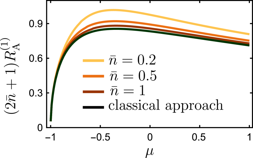
Figure 4: The scaled addition to the quantum activation energy $R_{\mathrm{A}}^{(1)}$ due to an extra drive as given by Eq. (24). The plot refers to switching from the stable state at $Q>0$ and to the phase of the extra drive $\varphi=\pi/2$; $\bar{n}$ is the thermal occupation number of the parametric oscillator, and $\mu=\omega_{p}(\omega_{p}-2\omega_{0})/F_{p}$.

The difference of the switching rates due to the extra drive leads to a difference in the stationary populations of the period-two states of the oscillator, see Sec. VII.1. For a classical parametrically modulated micromechanical resonator the population difference and its periodic dependence on $\varphi_{d}$ was observed in Ref. [28].

V.1 High-temperature limit

It is seen from Eq. (III) that, for a large thermal occupation number $\bar{n}$, the transition probabilities become symmetric, $\absolutevalue{W_{n+m\,n}-W_{n-m\,n}}\ll W_{n+m\,n}$. Then, from Eq. (12), the derivative of the activation energy becomes small, and we can expand $\xi\approx 1-\omega(g)R^{\prime}(g)+\left[\omega(g)R^{\prime}(g)\right]^{2}/2$. Inserting this expansion into Eq. (12) gives

$$R^{\prime}(g_{n})=2\omega^{-1}(g)\sum_{m}mW_{n+m\,n}\bigg{/}\sum_{m}m^{2}W_{n+m\,n}$$ (26)

Using the relation between the transition rates and the Fourier components of $a(\tau,g)$ [25], the above ratio for the well of $g(Q,P)$ at $Q>0$ can be written as

$$R^{\prime}(g)=\frac{2}{2\bar{n}+1}\frac{M(g)}{N(g)}\,,\qquad M(g)=\iint_{A(g)}d{}{Q}d{}{P}\,,$$

$$N(g)=\frac{1}{2}\iint_{A(g)}d{}{Q}d{}{P}\,(\partial_{Q}^{2}+\partial_{P}^{2})g(Q,P)\,,$$ (27)

where the integrals run over the interior of the well limited by the contour $g(Q,P)=g$. The relation (V.1) was derived in Ref. [25] in the absence of an extra drive at half the modulation frequency, but it applies also in the presence of such drive.

The correction $\alpha_{d}R^{\prime(1)}$ to $R^{\prime}(g)$ is determined by the corrections $\alpha_{d}M^{(1)}(g)$ and $\alpha_{d}N^{(1)}(g)$ to $M(g)$ and $N(g)$, respectively,

$$R^{\prime(1)}(g)=\frac{2}{2\bar{n}+1}\left[\frac{M^{(1)}(g)}{N^{(0)}(g)}-\frac{M^{(0)}(g)}{N^{(0)}{}^{2}(g)}N^{(1)}(g)\right].$$ (28)

To find these corrections we note first that $M=2\pi I_{f}$, where $I_{f}$ is the full action of the intrawell motion, see Sec. II.1 and Appendix A.1. Then from Eq. (50)

$$M^{(1)}=\pi\sin\varphi_{d}$$ (29)

Using, as in Appendix A.1 that, on the trajectory with a given $g=g^{(0)}+\alpha_{d}g^{(1)}$ and a given $Q$, the correction $\alpha_{d}P^{(1)}(Q|g)$ to the momentum is equal to $\alpha_{d}P^{(1)}=-\alpha_{d}g^{(1)}/\partial_{P}g^{(0)}$, one finds

$$N^{(1)}=\pi(\mu+2)\sin\varphi_{d}.$$ (30)

Equations (29) and (30) give the correction $R^{\prime}{}^{(1)}$ in the explicit form.

An important aspect of the calculation of $R^{\prime(1)}(g)$ in the limit $\bar{n}\gg 1$ is that it can be done using in Eq. (26) the general expressions for the corrections to the transition rates $W^{(1)}_{nn^{\prime}}$. Comparing the fairly cumbersome expressions for these corrections to the calculation in terms of $M^{(1)}$ and $N^{(1)}$ provides a way to independently check them. The calculation in Appendix D shows that the expressions obtained by two different approaches coincide.

The change of the activation energy for switching from the well at $Q>0$ is $\alpha_{d}R_{\mathrm{A}}^{(1)}$ with

$$R_{A}^{(1)} =\int_{g_{\text{min}}^{(0)}}^{0}R^{\prime(1)}(g)d{}g+\frac{2\sin\varphi_{d}\sqrt{1+\mu}}{(2\bar{n}+1)(2+\mu)}$$ (31)

The last term in the above expression is obtained from Eq. (V.1) by taking into account that the minimum of the $Q>0$-well is shifted from $g_{\mathrm{min}}^{(0)}$ by $-\sqrt{1+\mu}\sin\varphi_{d}$ and that, for $2\bar{n}+1\gg 1$, we have $R^{\prime}{}^{(0)}(g_{\mathrm{min}}^{(0)})\approx 2[(2+\mu)(2\bar{n}+1)]^{-1}$.

For large $\bar{n}$ we have $2/\lambda(2\bar{n}+1)\approx F\omega_{p}^{2}/6\gamma kT$. The Planck constant has dropped out from this expression. The result for $R_{\mathrm{A}}$ coincides with the expression derived within a classical formulation [27], except that the analytic expression for $M^{(1)}$ and $N^{(1)}$ were not obtained in [27].

V.2 Prebifurcation regime

Explicit expressions for $R^{\prime}$ and for $R_{\mathrm{A}}$ in the presence of an extra drive can be also obtained near the bifurcation point where there emerge the period-two states of the parametrically modulated oscillator. In the absence of dissipation and an extra drive, the bifurcation point is $\mu=-1$: for $\mu+1>0$ the Hamiltonian function $g^{(0)}(Q,P)$ has two minima that correspond to period-two states, whereas for $\mu<-1$ it has one minimum at $Q=P=0$.

Dissipation shifts the position of the bifurcation point, and in a close vicinity to the bifurcation point the oscillator motion is overdamped. The dynamics is controlled by a soft mode, a single dynamical variable that, in the quantum regime, satisfies a first order Langevin equation with the noise intensity $\propto(2\bar{n}+1)$ [41]. We show in Appendix E that this approach applies also in the presence of an extra drive and allows describing the effect of such drive on the activation energy of interwell switching.

For weak damping there exists a regime where the oscillator is close, but not too close to the bifurcation point. In the corresponding parameter range the motion is underdamped, on the one hand but, on the other hand, the switching rate and the effect of an extra drive on this rate display a characteristic scaling with the distance to the bifurcation point. We call this a prebifurcation regime, and the corresponding parameter range can be called the prebifurcation range. Where there is no extra drive, this range is easy to find by noting that the dimensionless frequency of vibrations about the minimum of $g^{(0)}(Q,P)$ is $\omega^{(0)}(g^{(0)}_{\mathrm{min}})=2(\mu+1)^{1/2}$. The prebifurcation range is where this frequency is small, $\omega^{(0)}(g^{(0)}_{\mathrm{min}})\ll 1$, yet it is much larger than the dimensionless decay rate $\kappa$.

For $\omega(g)\ll 1$, one can expand $\exp[-\omega(g)R^{\prime}(g)]$ in Eq. (12), which results in Eq. (26) for $R^{\prime}(g)$ and ultimately in the expressions (V.1) - (31) for $R^{\prime}(g)$ and for the corrections to $R^{\prime}$ and $R_{A}$ due to the extra drive. We emphasize that these expressions apply even where $\bar{n}<1$, the only condition is that the system is close to the bifurcation point. It is easy to show that in the prebifurcation range $N^{(0)}(g)\approx M^{(0)}(g)$. Taking into account that $g^{(0)}_{\mathrm{min}}=-(\mu+1)^{2}/4$ we obtain from Eq. (V.1) $R_{\mathrm{A}}^{(0)}\approx(\mu+1)^{2}/2(2\bar{n}+1)$ [25], whereas from Eqs. (29) - (31) for the well with $Q>0$

$$R_{\mathrm{A}}^{(1)}\approx\frac{2\sin\varphi_{d}}{2\bar{n}+1}\sqrt{\mu+1},\quad\mu+1\ll 1.$$ (32)

Interestingly, the correction to the switching rate (32) falls off with the decreasing distance to the bifurcation point $\mu+1$ much slower than the leading term $R_{\mathrm{A}}^{(0)}$. This shows that the range of applicability of the perturbation theory shrinks down as the system approaches the bifurcation point. We note that both $R_{\mathrm{A}}^{(0)}$ and $R_{\mathrm{A}}^{(1)}$ depend on $\bar{n}$ in the same way, $\propto 1/(2\bar{n}+1)$.

VI BREAKING OF THE PERTURBATION THEORY AND OF THE DETAILED BALANCE FOR $\bar{n}=0$

The form of the distribution over the intrawell states far from the bottom of the well strongly depends on the probabilities of transitions between remote levels, i.e., on $W_{n\,n+m}$ with large $m>0$. The transitions $n\to n+m$ with $m>0$ directly “populate” the excited states. In the cases we consider here important are transitions where $m$ is not too large, so that the rates $W_{n\,n+m}$ are not too small. Then they are still determined by the matrix elements of $\hat{a}$-operator expressed in terms of the Fourier components $a_{m}(g)$, cf. Eqs. (III) and (III).

The functions $a_{m}(g)$ fall off exponentially with the increasing $|m|$. In particular, with no extra drive [25],

$$|a_{m}^{(0)}|\approx k(g)\exp(-\beta_{>}m),\qquad m\gg 1$$

$$|a_{m}^{(0)}|\approx k(g)\exp(-\beta_{<}|m|),\qquad-m\gg 1.$$ (33)

Both $\beta_{>}\equiv\beta_{>}(g)$ and $\beta_{<}\equiv\beta_{<}(g)$ depend on $g$, whereas $k(g)\propto\kappa\omega^{(0)}(g)$ is a smooth function of $g$. The explicit form of the parameters $\beta_{\lessgtr}$ is given in Appendix A. It is important that $\beta_{>}>\beta_{<}$. Therefore the parameters $(W^{\mathrm{(e)}}_{n+m\,n})^{(0)}\propto|a_{-m}^{(0)}(g_{n})|^{2}$, which give the rates of transitions $n+m\to n$ for $\bar{n}=0$ and no extra drive, meet the condition $(W_{n+m\,n}^{\mathrm{(e)}})^{(0)}>(W_{n\,n+m}^{\mathrm{(e)}})^{(0)}$ for $m>0$. The latter condition shows that the oscillator is more likely to move toward smaller $n$, i.e., toward the minimum of $g(Q,P)$, which is consistent with this minimum being a stable state in the presence of dissipation.

An important consequence of Eq. (VI) and of the general expressions for $a_{m}^{(0)}(g)$, Eq. (A), is that the rates $(W_{nn^{\prime}}^{\mathrm{(e)}})^{(0)}$ meet the detailed balance condition for the transition rates

$$W_{nn^{\prime}}W_{n^{\prime}n^{\prime\prime}}W_{n^{\prime\prime}n}=W_{nn^{\prime\prime}}W_{n^{\prime\prime}n^{\prime}}W_{n^{\prime}n}\,,$$ (34)

which is the condition of the independence of the “path” followed in consecutive transitions along a loop that takes the system back to the initial state. In turn, a consequence of the detailed balance condition is that the function $R^{\prime}(g)$, which determines the distribution over the intrawell states, has a simple form. As seen from Eqs. (12) and (VI), for $\bar{n}=0$ and no extra drive

$$R^{\prime}{}^{(0)}_{\bar{n}=0}(g) =2\omega^{-1}(g)[\beta_{>}(g)-\beta_{<}(g)].$$ (35)

[we use here and below in this and the following section that $\omega(g)\approx\omega^{(0)}(g)$].

The rates $W^{\mathrm{(e)}}_{n+m\,n}$ are determined by interstate transitions with emitting excitations into the thermal bath, and therefore they are nonzero even when there are no bath excitations with energy $\hbar\omega_{0}$, so that $\bar{n}=0$. In contrast, the rates $W^{\mathrm{(abs)}}_{n+m\,n}$ are determined by absorption of excitations. In the absence of an extra drive, $(W^{\mathrm{(abs)}}_{n+m\,n})^{(0)}\propto\bar{n}|a_{m}^{(0)}(g)|^{2}$. Clearly, the detailed balance condition is not satisfied if both transition rates contribute to the total transition rate, i.e., if $(W_{n+m\,n})^{(0)}=(W^{\mathrm{(e)}}_{n+m\,n})^{(0)}+(W^{\mathrm{(abs)}}_{n+m\,n})^{(0)}$. In this case $R^{\prime}{}^{(0)}(g)$ has to be found numerically from Eq. (12) [25].

From Eq. (VI), the rate of the absorption-induced transitions $n\to n+m$ falls off with the increasing $m>0$ exponentially slower than the rate of the emission-induced transitions. This is why the absorption-induced transitions dramatically change the distribution over the states even for small $\bar{n}>0$, as the ratio $(W^{\mathrm{(abs)}}_{n\,n+m})^{(0)}/(W^{\mathrm{(e)}}_{n\,n+m})^{(0)}$ becomes large for large $m>0$.

Formally, the effect can be seen by looking at the term $\sum_{m}W_{n\,n+m}\exp[m\omega(g_{n})R^{\prime}(g_{n})]$ in Eq. (12) for $R^{\prime}$ and considering the transition rates $(W^{\mathrm{abs)}}_{n\,n+m})^{(0)}$ as a perturbation. If one uses $R^{\prime}$ from Eq. (35), one sees that, for $m\gg 1$,

$$(W^{\mathrm{(abs)}}_{n\,n+m})^{(0)}\exp[m\omega(g_{n})R^{\prime}{}^{(0)}_{\bar{n}=0}(g_{n})]$$

$$\propto\exp\{2m[\beta_{>}(g_{n})-2\beta_{<}(g_{n})].\}$$ (36)

For the sum of these terms to converge one has to have $\beta_{>}-2\beta_{<}<0$. This condition breaks down for a part of the intrawell states once $\mu>-1/2$ [25]. As a result, even for very small $\bar{n}$, $R^{\prime}{}^{(0)}$ is much smaller than what follows from Eq. (35) and, respectively, the population of higher intrawell states is exponentially larger than for $\bar{n}=0$.

It is important that the condition $\beta_{>}(g)-2\beta_{<}(g)<0$ breaks down with the increasing $\mu>-1/2$ first near the local maximum of $g(Q,P)$ at $g=0$. As $\mu$ increases beyond $-1/2$ the range of $g$ where $\beta_{>}(g)-2\beta_{<}(g)>0$ is also increasing.

VI.1 Nonanalytic effect of a weak extra drive for $\bar{n}=0$

The extra drive at frequency $\omega_{p}/2$ changes the parameters $a_{m}(g)$. It admixes to $a_{m}^{(0)}$ Fourier components $a^{(0)}_{k}{}$ with different $k{}$, see Eq. (IV.2). Therefore, even for $\bar{n}=0$, where the transition rates are $W^{\mathrm{(e)}}_{n\,n+m}\propto|a_{m}(g_{n})|^{2}$, the expressions for these rates have the terms that contain $a^{(0)}_{k}{}$ with positive and negative $k{}$. The presence of the terms $a^{(0)}_{k}{}$ with $k{}<0$ in $W^{\mathrm{(e)}}_{n\,n+m}$ for $m>0$ can lead to a breakdown of the perturbation theory with respect to the scaled extra-drive amplitude $\alpha_{d}$. Indeed, for large $m$ the terms $\propto\alpha_{d}a_{k{}<0}^{(0)}$ admixed to $a_{m>0}^{(0)}$ can become comparable to the terms $a_{m>0}^{(0)}$ themselves.

To see how the breakdown occurs we note that the coefficients $J_{mk},L_{mk}$ in Eq. (IV.2) are linear combinations of the terms $\propto a_{k}^{(0)}$ and $a_{-k}^{(0)}$, cf. Eqs. (B) and (B) in Appendix B. The leading-order term in the correction $|a_{m}^{(1)}|$ for large $m$ comes from the term $a_{-k}^{(0)}$ with $k\approx m$ in Eq. (IV.2), and then $|a_{m}^{(1)}|\propto\exp(-\beta_{<}m)$. This is the same dependence on $m$ as displayed by $a_{-m}^{(0)}$ and that leads to the breaking of the detailed balance by the transition rates $(W^{\mathrm{(abs)}}_{n\,n+m})^{(0)}\propto\bar{n}$ in the absence of the extra drive.

The slow decay of $a_{m}^{(1)}$ requires evaluating and incorporating the correction $\propto\alpha_{d}^{2}$ in the transition rates. Indeed, for large $m$, as seen from Eq. (IV.3), the correction $\alpha_{d}(W^{\mathrm{(e)}}_{n\,n+m})^{(1)}$ falls off as $\exp[-(\beta_{>}+\beta_{<})m]$. On the other hand, the second-order correction $\propto\alpha_{d}^{2}|a_{m}^{(1)}|^{2}\propto\exp(-2\beta_{<}m)$ falls off much slower and becomes dominating for large $m$. This shows that, for large $m$ and for $\bar{n}=0$, the correction to $W^{\mathrm{(e)}}_{n\,n+m}$ is

$$\alpha_{d}^{2}\tilde{W}^{\mathrm{(e)}}_{n\,n+m}\approx 2\kappa\alpha_{d}^{2}|a_{m}^{(1)}|^{2}\propto\exp(-2\beta_{<}m),\quad m\gg 1.$$ (37)

Generally, if one keeps a quadratic in $\alpha_{d}a_{m}^{(1)}$ term in $|a_{m}|^{2}$, one should also incorporate the second-order term $\propto\alpha_{d}^{2}a_{m}^{(2)}$ into Eq. (IV.2) for $a_{m}$. However, $|a_{m}^{(2)}|$ falls off with the increasing $m$ as $\exp(-\beta_{<}m)$ (clearly, there is no slower rate of the falloff, but this has been also confirmed by a calculation). Therefore its contribution to $|a_{m}|^{2}$, which is $\propto\alpha_{d}^{2}|a_{m}^{(0)}a_{m}^{(2)}|\propto\exp[-(\beta_{>}+\beta_{<})m]$ to the leading order in $\alpha_{d}$, is exponentially smaller than that of $\alpha_{d}^{2}|a_{m}^{(1)}|^{2}$ for $\beta_{>}>\beta_{<}$ and $m\gg 1$.

VI.1.1 The probability distribution

Equation (37) shows that, in the presence of the extra drive, even for $\bar{n}=0$ the intrawell distribution is no longer described by the simple detailed-balance expression (35). To find the distribution for $\bar{n}=0$ and small $\alpha_{d}$ one has to use Eq. (12) with the transition rate

$$W^{\mathrm{(e)}}_{n\,n+m}= (W^{\mathrm{(e)}}_{n\,n+m})^{(0)}+\alpha_{d}(W^{\mathrm{(e)}}_{n\,n+m})^{(1)}$$

$$+\alpha_{d}^{2}\tilde{W}^{\mathrm{(e)}}_{n\,n+m}.$$ (38)

Since $\tilde{W}^{\mathrm{(e)}}_{n\,n+m}$ has the same asymptotic behavior for large $m$ as $(W^{\mathrm{(abs)}}_{n\,n+m})^{(0)}$, it leads to a sharp jump in the value of $R^{\prime}$ for $\bar{n}=0$, which is similar to the jump due to a nonzero $\bar{n}$ in the absence of the extra drive. In the range $\beta_{>}(g)>2\beta_{<}(g)$ these are the transition rates $\alpha_{d}^{2}\tilde{W}^{\mathrm{(e)}}_{n\,n+m}$ that control the distribution over the intrawell states. The solution of Eqs. (12), (37), and (VI.1.1) for $R^{\prime}(g)$ in this range has the form

$$R^{\prime}_{\alpha_{d}}(g)= 2[\beta_{<}(g)-\epsilon]/\omega^{(0)}(g),\quad 0<\epsilon\ll 1,$$

$$\beta_{>}(g)>2\beta_{<}(g)$$ (39)

Plugging this Ansatz into Eq. (12) for $\bar{n}=0$, taking into account that, in this equation the term

$$\sum_{m}(W^{\mathrm{(e)}}_{n\,n+m})^{(0)}\{1-\exp[m\omega(g_{n})R^{\prime}_{\alpha_{d}}(g_{n})]\}\sim\kappa\omega^{2}(g_{n})/\lambda$$

remains finite for $\beta_{>}>\beta_{<}$, and noting that

$$\sum_{m}\tilde{W}^{\mathrm{(e)}}_{n\,n+m}\{1-\exp[m\omega(g_{n})R^{\prime}_{\alpha_{d}}(g_{n})]\}\sim\kappa\omega^{2}(g_{n})/\lambda\epsilon,$$

one finds from the stationarity condition $\sum_{m}W^{\mathrm{(e)}}_{n\,n+m}\{1-\exp[m\omega(g_{n})R^{\prime}_{\alpha_{d}}(g_{n})]\}=0$ that, to the lowest order in $\alpha_{d}^{2}$,

$$\epsilon\sim\alpha_{d}^{2}.$$

This justifies the assumption $\epsilon\ll 1$ for a weak extra drive.

The relation $R^{\prime}_{\alpha_{d}}(g)<R^{\prime}{}^{(0)}_{\bar{n}=0}$ shows that the stationary distribution over the intrawell states falls off exponentially slower in the presence of an extra drive than without such drive. This is an unexpected nonperturbative effect of the drive.

VI.1.2 Logarithmic susceptibility vs nonperturbative effect of the drive

For nonzero $\bar{n}$ and in the presence of the extra drive, in the expression for the transition rate one has to take into account both the absorption-induced term $W^{\mathrm{(abs)}}_{n\,n+m}$ and the drive-induced modification of the emission term (VI.1.1). In the regime where $\bar{n}\gg\lambda$ and $\alpha_{d}\ll 1$ the effect of the extra drive can be captured already by the linear corrections to the transition probabilities. This results in the logarithmic susceptibility discussed in Sec. V. On the other hand, for $\bar{n}\lesssim\lambda\ll\alpha_{d}^{2}$ the extra drive completely modifies the probability distribution.

Different regimes of the response to the extra drive are sketched in Fig. 5. For a very small drive amplitude, $\alpha_{d}\lesssim\lambda$, the drive is just a small perturbation which weakly affects the distribution over the states. However, once the scaled amplitude becomes much larger than the scaled Planck constant, $\alpha_{d}\gg\lambda$, it affects the distribution exponentially strongly, and the effect very strongly depends on the thermal occupation number of the oscillator $\bar{n}$.

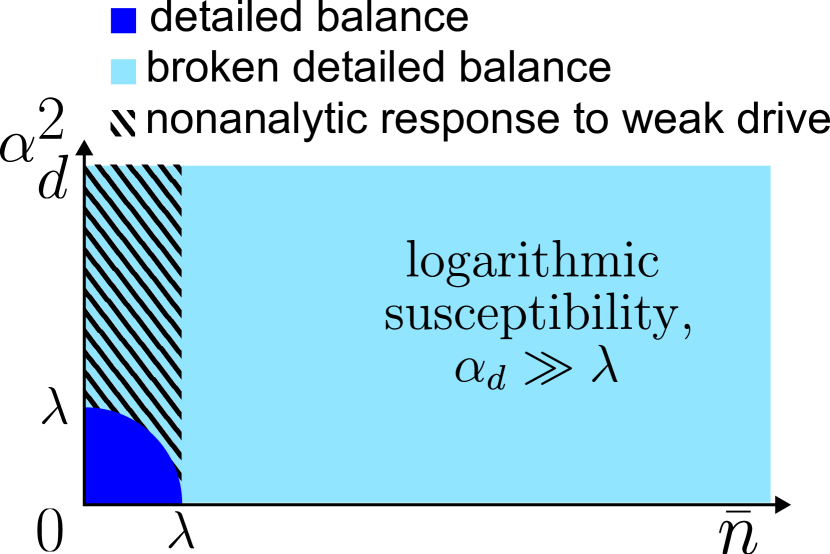
Figure 5: The regions where the effect of a weak extra force on the oscillator dynamics are qualitatively different. Where $\bar{n}$ and the scaled squared force amplitude $\alpha_{d}^{2}$ are small compared to the effective Planck constant $\lambda$, the oscillator has detailed balance. The detailed balance is broken outside this region. For $\bar{n}\gg\lambda$ a major effect of the weak extra force is the linear in $\alpha_{d}$ change of the switching rate, which is described by the logarithmic susceptibility,

VI.2 Detailed balance and the potential condition

The breaking of detailed balance in a parametric oscillator by an extra drive at frequency $\omega_{p}/2$ for $\bar{n}=0$ has a broader implication. To see it we note that the dynamics of the oscillator can be described in the complex $P$-representation of quantum optics, where the density matrix is determined by the function $P(\alpha,\beta)$ in the basis of coherent states $\ket{\alpha},\ket{\beta}$. The equation for the function $P$ has the form of the Fokker-Planck equation, i.e., a diffusion equation

$$\partial_{t}P=-{\bm{\nabla}}({\bf j}P)+\frac{1}{2}\sum_{i,j=\alpha,\beta}\partial_{i}\partial_{j}D^{ij}P,$$

where ${\bf j}\equiv(j_{\alpha},j_{\beta})$ can be associated with the drift current in the $(\alpha,\beta)$-space and $D^{ij}$ is the coefficient of diffusion in this space; both ${\bf j}$ and $D^{ij}$ are functions of $\alpha,\beta$. Interestingly, the stationary solution of this equation can be found by setting the total current, i.e., the sum of the drift and diffusion current, equal to zero, $j_{i}P+\sum_{j}\partial_{j}D^{ij}P=0$. The matrix $D^{ij}$ is diagonal, so that the latter equation is easily solved for each $i$ [4], giving $P$ in the “quasi-Boltzmann” form, $P=\exp[-\phi(\alpha,\beta)]$. The cross-derivatives of $\phi$ calculated this way are equal to each other, the condition called the potential condition. This condition is usually associated with detailed balance.

The results of Sec. VI.1 show that, actually, an extra force at frequency $\omega_{p}/2$ breaks the detailed balance displayed by a parametric oscillator for $\bar{n}=0$ even though the potential condition holds. On physical grounds, there are no reasons to expect that a parametric oscillator would have detailed balance, since the system is far from thermal equilibrium. From this point of view, the result is not unexpected, but it shows that the fact that the stationary $P$ representation of the density matrix meets the potential condition is not an indicator of the presence of detailed balance. An interesting extension of the concept of detailed balance was developed and applied to a parametric oscillator in Refs. [10, 12]; it enabled, in particular, to develop an alternative way of finding the stationary distribution of the oscillator.

VII Nonanalytic change of the switching rates by an extra drive for $\bar{n}=0$

The change of the distribution over the states within a well of $g(Q,P)$ by the extra drive leads to a change of the populations of the states near the barrier top, $g=0$, and thus to a change of the switching rate. This change is given by the change of the effective activation energy $R_{\mathrm{A}}=R(g=0)$, cf. Eq. (13). We now consider it for $\bar{n}=0$. In this case, as explained in Sec. VI.1, for $\mu>-1/2$ the drive leads to exponentially larger probabilities of transitions into highly excited intrawell states than in the absence of the drive. Respectively, the correction to $R_{\mathrm{A}}=\int_{g_{\mathrm{min}}}^{0}R^{\prime}(g)dg$ does not have the form of a series in the scaled drive amplitude $\alpha_{d}$.

There are three regions of $g$ that contribute to the integral that gives $R_{\mathrm{A}}$, cf. Eq. (V): (i) the region between the shifted minimum $g_{\mathrm{min}}$ of $g(Q,P)$ and the unperturbed minimum $g_{\mathrm{min}}^{(0)}$; (ii) the region between $\mathrm{max}(g_{\mathrm{min}},g_{\mathrm{min}}^{(0)})$ and the critical value $g_{c}$ given by the condition

$$\beta_{>}(g_{c})=2\beta_{<}(g_{c}),$$

and (iii) the region $g_{c}<g<0$ where $\beta_{>}(g)>2\beta_{<}(g)$. The value of $g_{c}$ is well-approximated by $-(1+2\mu)/XXX$.

Equation (V) explicitly describes the contribution from the region (i). In the region (ii) one can find the correction $R^{\prime}{}^{(1)}$ to $R^{\prime}$ from Eq. (21). In the region (iii) $R^{\prime}$ is given by Eq. (VI.1.1). Because in this region $R^{\prime}(g)=R^{\prime}_{\alpha_{d}}(g)\ll R^{\prime}{}^{(0)}(g)$, the overall activation energy $R_{\mathrm{A}}$ is much smaller than in the absence of the extra drive.

We note that, strictly speaking, the discrete WKB approximation (11) breaks down in a narrow region around $g_{c}$, as this approximation relies on the smoothness of the scaled logarithm of the distribution over the intrawell states $R(g_{n})=-\lambda\log\rho_{n}$, whereas $d^{2}R/dg^{2}$ is discontinuous at $g_{c}$. The distribution $\rho_{n}$ for the states with $|g_{n}-g_{c}|\sim\lambda$ has to be analyzed more carefully. However, since the width of the region is $\sim\lambda$, the correction to $R(g)$ is $\sim\lambda$, i.e., it only affects the prefactor in the distribution, cf. [42].

A careful numerical analysis of the corrections to the rates of transitions between the intrawell states $W_{n+m\,n}^{(1)}$ given by Eq. (IV.3) shows that, for $\bar{n}=0$, in a fairly broad range of $|m|$ the ratio $W_{n+m\,n}^{(1)}/W_{n+m,\,n}^{(0)}$ for $m>0$ is the same as for $m<0$. Since the rates fall off exponentially with the increasing $|m|$ and, by construction, the numerator in the expression (21) for $R^{\prime}{}^{(1)}$ is zero if we replace $W_{n+m\,n}^{(1)}$ with $W_{n+m,\,n}^{(0)}$, the value of $R^{\prime}{}^{(1)}$ is very small. This property holds only for $\bar{n}=0$, where $W_{n+m,\,n}\equiv W^{(e)}_{n+m,\,n}{}$. As a result, the linear in $\alpha_{d}$ correction to $R_{\mathrm{A}}$ is

$$R_{\mathrm{A}}^{(1)}\approx\delta R_{\mathrm{A}}^{\mathrm{lin}}=(g_{\mathrm{min}}^{(0)}-g_{\mathrm{min}})R^{\prime}{}^{(0)}_{\mathrm{min}}\quad(\bar{n}=0),$$ (40)

where $g_{\mathrm{min}}$ and $R^{\prime}{}^{(0)}_{\mathrm{min}}$ are given by Eqs. (7) and (22), respectively. Clearly, $\delta R_{\mathrm{A}}^{\mathrm{lin}}\propto\alpha_{d}$.

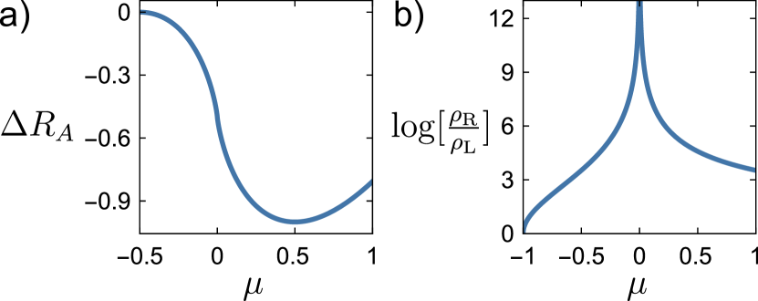
Figure 6: (a) The leading term in the change of the quantum activation energy $\Delta R_{A}$, Eq. (VII) due to the nonperturbative effect of the extra force for $\bar{n}=0$. (b) Logarithm of the ratio of the stationary populations $\rho_{R}/\rho_{L}$ of the wells of the Hamiltonian function $g(Q,P)$ as a function of the frequency detuning parameter $\mu$ for the scaled amplitude of the extra force $\alpha_{d}\sin(\varphi_{d})/\lambda=1$ and $\bar{n}=0$. The well populations are the populations of the states of parametrically excited vibrations of the oscillator.

Figure 6 (a) shows the leading term in the change of the activation energy due to the weak extra drive for $\bar{n}=0$,

$$\Delta R_{\mathrm{A}}=2\int_{g_{c}}^{0}dg\,[2\beta_{<}(g)-\beta_{>}(g)]/\omega^{(0)}(g)$$

$$\approx R_{\mathrm{A}}-R_{\mathrm{A}}^{(0)}-\delta R_{\mathrm{A}}^{\mathrm{lin}}.$$ (41)

Here in the second line we disregarded the correction $\epsilon\propto\alpha_{d}^{2}$ in Eq. (VI.1.1) for $R^{\prime}_{\alpha_{d}}(g)$. The change $\Delta R_{\mathrm{A}}$ is negative, the extra drive significantly decreases the activation energy for switching between the oscillator states, with the decrease being independent of the drive amplitude (still we assume $\alpha_{d}\gg\lambda$).

VII.1 The stationary distribution

Over time, switching between the wells of $g(Q,P)$ leads to a stationary distribution over the wells, i.e., over the states of parametrically excited vibrations with the opposite phases. If we use subscripts $L$ and $R$ for the wells of $g(Q,P)$ with $Q<0$ and $Q>0$, respectively, the stationary well populations $\rho_{L,R}$ are inversely proportional to the rates of switching from the corresponding wells, $W_{\mathrm{L\to R}}$ and $W_{\mathrm{R\to L}}$,

$$W_{\mathrm{L\to R}}\rho_{\mathrm{L}}=W_{\mathrm{R\to L}}\rho_{\mathrm{R}}\,.$$ (42)

The values of $W_{\mathrm{L\to R}}$ and $W_{\mathrm{R\to L}}$ are given by Eq. (13) for $W_{\mathrm{sw}}$ with $R_{\mathrm{A}}$ calculated for the left and right wells, respectively. A weak extra drive makes the rate exponents $R_{\mathrm{A}}/\lambda$ different. For a weak extra drive, the difference comes from the term $R_{\mathrm{A}}^{(1)}$, which is linear in the drive amplitude and has opposite signs in the different wells. The term $\Delta R_{\mathrm{A}}$, which may be much larger than $|R_{\mathrm{A}}^{(1)}|$ for $\bar{n}=0$, has the same sign in the both wells and does not change the ratio of the switching rates.

As a result, $\log[\rho_{\mathrm{R}}/\rho_{\mathrm{L}}]$ linearly depends on the amplitude of the extra drive. The dependence on $\mu$ and $\bar{n}$ for $\bar{n}\gg\lambda$ is clear from Fig. 4. On the other hand, for $\bar{n}=0$ we have

$$\log[\rho_{\mathrm{R}}/\rho_{\mathrm{L}}] \approx\frac{\alpha_{d}}{\lambda}\sin\varphi_{d}\log(\frac{\mu+2+2\sqrt{1+\mu}}{\mu+2-2\sqrt{1+\mu}})\,.$$ (43)

This ratio coincides with the result of Refs. [4, 12] for the stationary distribution for $\bar{n}=0$ if one considers the limit of weak damping, weak drive and small effective Planck constant $\lambda$ in the above papers. However, the switching rates, wich are the subject of the present paper, were not considered in that work.

The ratio (43) as function of $\mu$ is shown in Fig. 6. Characteristically, for $\alpha_{d}\gg\lambda$ the weak drive can lead to an exponentially large imbalance of the populations of the wells. The phase of the drive $\varphi_{d}$ controls which well is favored.

We note that, for $\mu\rightarrow 0$, the imbalance of the populations diverges for $\bar{n}=0$. However, the probability of a transition from the lowest intrawell state to a higher state goes to zero in the considered model, that is, the oscillator “freezes” in the lowest intrawell state. Other dissipation mechanisms can break this freezing. An example is dephasing due to quasielastic scattering of bath excitations from the oscillator. It leads to a nonzero probability of transitions from the lowest intrawell state to higher states [25].

VIII Conclusion

The results of this paper reveal unexpected aspects of quantum fluctuations in parametric oscillators that, at least in part, go beyond the considered model. The model itself is well-known and broadly used: a weakly nonlinear oscillator, which is parametrically modulated at frequency $\omega_{p}$ close to twice the eigenfrequency and additionally driven by a weak force at frequency $\omega_{p}/2$. Without this force, the oscillator dynamics in the frame rotating at frequency $\omega_{p}/2$ is described by a symmetric double-well Hamiltonian, with the symmetry related to the time shift by the modulation period $2\pi/\omega_{p}$. The force with twice this period lifts the symmetry. It thus suppresses the tunneling between the symmetric states. One might expect that this would localize the oscillator inside the wells.

The physical picture is qualitatively different in the presence of relaxation. The coupling of the oscillator to a thermal bath leads to dissipation and also to quantum fluctuations. In turn, these fluctuations lead to the inter-well switching in which the oscillator goes over the barrier that separates the wells. This is reminiscent of thermal activation, except that the activation can be caused by quantum fluctuations and can occur for $T=0$.

Our results show that the force at frequency $\omega_{p}/2$ can exponentially increase the switching rate. This may be thought of as a reduction of the barrier height. However, the actual process is more delicate, as the system is far from thermal equilibrium and the conventional picture on quasi-Boltzmann distribution over the intrawell states is entirely inadequate.

Our analysis refers to the case where the wells of the Hamiltonian contain many states, but the decay rate of the oscillator is small, so that the level spacing largely exceeds the level widths. In this case, as we show, the major effect of the extra force is the change of the rates of transitions between the intrawell states. It can be thought of as the change of the random walk over the intrawell states due to quantum fluctuations. Ultimately, this change results in a change of the probability to reach the top of the barrier that separates the wells and then to switch to another well. Because there are many states involved and the effect of the change accumulates, the change of the rate of interwell switching is exponential in the force amplitude.

The strength of the effect comes from the fact that, in the exponent of the switching rate, the amplitude of the extra force is multiplied by the number of the intrawell states. We find the relevant factor. The general expression simplifies for comparatively large thermal occupation number of the oscillator $\bar{n}$, in which case the above factor is $\propto(2\bar{n}+1)^{-1}$. It also simplifies near a bifurcation point, where the factor is shown to scale as the distance to the bifurcation point to the power $1/2$.

Arguably, the most interesting results refer to the case where one can set $\bar{n}=0$. This case is of primary interest for many applications of quantum parametric oscillators. Here, for the most frequently used model of dissipation, fluctuations in the oscillator meet the detailed balance condition, in the absence of an extra drive. We show that even a comparatively weak extra force breaks this condition. This results in a very strong increase of the switching rate, with the leading term in the exponent being independent of the force amplitude. In a sense, the rate change is not just exponentially strong, but also nonperturbative.

A delicate feature of the result for $\bar{n}=0$ is that the oscillator dynamics, as described in the coherent-state representation by the commonly used Glauber-Sudarshan function $P(\alpha,\alpha^{*})$, satisfies the so-called potential condition. This means that, in the stationary state, the current (and not just the divergence of the current) described by $P(\alpha,\alpha^{*})$ is zero. Our observation shows that, even though the current is still zero in the stationary state in the presence of an extra force, there is no detailed balance. The product of the rates of a sequence of transitions that start from a given quantum state and bring the system back to the same state depends on the intermediate states.

The strong effect of the extra force on the rate of switching between the vibrational states of a quantum oscillator suggests a way of an efficient control of such switching. In particular, the possibility to increase the switching rate is important for applications. Our results also provide the means for analyzing the dynamics of networks of coupled quantum parametric oscillators, where the major effect of the coupling is the force that vibrations of the coupled oscillators exert on each other. For different oscillators, such a network provides a quantum nonreciprocal system, since the forces between different oscillators are unbalanced if the vibrations have different amplitudes.

Appendix A CLASSICAL MOTION

We calculate the matrix elements $a_{m}(g_{n})=\braket{n+m}{\hat{a}}{n}$ in the semiclassical approximation. To this end, we consider the classical motion inside the wells. This is a periodic motion with frequency $\omega(g)$ that depends on the RWA energy $g$. It is described by the Hamiltonian equations

$$\frac{dQ}{d\tau} =\frac{\partial g}{\partial P}\,,\qquad\frac{dP}{d\tau}=-\frac{\partial g}{\partial Q}\,.$$ (44)

In the absence of extra drive the Hamiltonian of the system is $g^{(0)}$, and we write it as a function of the coordinate $q$ and momentum $p$, i.e., as $g^{(0)}(q,p)$. The Hamiltonian equations for $q,p$ have the form (44) with $g$ replaced with $g^{(0)}$,

$$dq/d\tau=\partial_{p}g^{(0)},\quad dp/d\tau=-\partial_{q}g^{(0)}.$$ (45)

The solution of these equations for the well at $q>0$ is expressed in terms of the Jacobi elliptic functions [25],

$$q(\tau,g) =\frac{2^{3/2}\absolutevalue{g}^{1/2}\operatorname{dn}(\tau^{\prime}|m_{J})}{\varkappa_{+}+\varkappa_{-}\operatorname{cn}(\tau^{\prime}|m_{J})}\,,$$

$$p(\tau,g) =\frac{\varkappa_{+}\varkappa_{-}\absolutevalue{g}^{1/4}\operatorname{sn}(\tau^{\prime}|m_{J})}{\varkappa_{+}+\varkappa_{-}\operatorname{cn}(\tau^{\prime}|m_{J})}\,,$$ (46)

where

$$\varkappa_{\pm} =(1+\mu\pm 2\absolutevalue{g}^{1/2})^{1/2}\,,\qquad\tau^{\prime}=2^{3/2}\absolutevalue{g}^{1/4}\tau\,,$$

$$m_{J} \equiv m_{J}(g,\mu)=\frac{(\mu+1-2\absolutevalue{g}^{1/2})(\mu-1+2\absolutevalue{g}^{1/2})}{8\absolutevalue{g}^{1/2}}\,$$

(here we use $\varkappa_{\pm}$ insetad of $\kappa_{\pm}$ used in [25] to avoid confusion with the relaxation rate parameter $\kappa$).

The Jacobi elliptic functions are double-periodic. The real period is $\tau_{p}^{(1)}=2^{1/2}\absolutevalue{g}^{-1/4}K(m_{J})$, whereas the second period is complex, $\tau_{p}^{(2)}=i2^{1/2}\absolutevalue{g}^{-1/4}K(1-m_{J})$; here $m_{J}\equiv m_{J}(g,\mu)$ is the modulus and $K(m_{J})$ is the complete elliptic integral of the first kind. The frequency of the classical motion in the absence of an extra drive is $\omega^{(0)}(g)=2\pi/\tau_{p}^{(1)}$. The double-periodicity of the Jacobi elliptic functions allows finding the Fourier components $a_{m}^{(0)}(g)$ of $a^{(0)}(\tau,g)=\left[p(\tau,g)-iq(\tau,g)\right]/\sqrt{2\lambda}$, i.e., the Fourier components $a_{m}(g)$ in the absence of the extra drive,

$$a^{(0)}_{m}(g)=-i(2\lambda)^{-1/2}\omega^{(0)}(g)\frac{\exp(-im\phi_{\ast})}{1+\exp(-im\phi_{0})}\,,$$

$$\phi_{0}=\pi\left(1+\tau_{p}^{(2)}/\tau_{p}^{(1)}\right)\,,$$ (47)

with $\phi_{\ast}$ given by the equation

$$\operatorname{cn}(2K\phi_{\ast}/\pi|m_{J})=-\left(\frac{1+\mu+2\absolutevalue{g}^{1/2}}{1+\mu-2\absolutevalue{g}^{1/2}}\right)^{1/2}\,.$$

The Fourier coefficients $a_{m}^{(0)}$ decay exponentially for large $\absolutevalue{m}$,

$$a_{m}^{(0)} \propto\exp(-m\Im{\phi_{0}-\phi_{\ast}})\,, m \gg 1\,,$$

$$a_{m}^{(0)} \propto\exp(-\absolutevalue{m}\Im{\phi_{\ast}})\,, -m \gg 1\,.$$ (48)

The exponents in this equation give the fall-off parameters of $a_{m}^{(0)}$ in Eq. (VI),

$$\beta_{>}=\imaginary(\phi_{0}-\phi_{\ast}),\quad\beta_{<}=\imaginary\phi_{\ast}.$$

Since $\Im{\phi_{0}-\phi_{\ast}}>\Im{\phi_{\ast}}$, the terms with positive $m$ in Eq. (A) decay faster than the ones with negative $m$, that is, $\beta_{>}>\beta_{<}$.

A.1 Frequency of intrawell vibrations

An extra drive at $\omega_{p}/2$ changes the shape of the wells of $g(Q,P)$ and the frequency of the intrawell vibrations. The reciprocal frequency as function of the energy $g$ is given by the derivative of the action $I_{f}(g)=(2\pi)^{-1}\oint P(Q|g)\,dQ$ over $g$, where $P(Q|g)$ is the momentum on the Hamiltonian trajectory (44) with a given $g$. The action $I_{f}$ and the momentum $P$ refer to the full time-independent RWA Hamiltonian. Therefore $I_{f}$ is independent of time, in contrast to the action variable $I(\tau)$ defined for the Hamiltonian $g^{(0)}$.

To the first order in $\alpha_{d}$, the action $I_{f}$ is determined by the linear in $\alpha_{d}$ correction to the momentum, $P(Q|g)\approx P^{(0)}(Q|g)+\alpha_{d}P^{(1)}(Q|g)$. Since the zeroth-order term $P^{(0)}(Q|g)$ is given by the equation $g^{(0)}(Q,P^{(0)})=g$, from Eq. (II) we find $I_{f}\approx I_{f}^{(0)}+\alpha_{d}I_{f}^{(1)}$ with

$$I^{(1)}_{f}(g)= -\frac{1}{2\pi}\oint dQ\,\frac{g^{(1)}\bigl{(}Q,P^{(0)}(Q|g)\bigr{)}}{\partial_{P}g^{(0)}},$$

$$= \frac{1}{2\pi}\int_{0}^{2\pi/\omega^{(0)}(g)}\left[P^{(0)}(\tau,g)\cos\varphi_{d}\right.$$

$$\left.+Q^{(0)}(\tau,g)\sin\varphi_{d}\right]d{}{\tau}\,,$$ (49)

where $Q^{(0)}(\tau,g)=q(\tau,g)$ and $P^{(0)}(\tau,g)=p(\tau,g)$ are the dynamical variables in the absence of the extra drive described by Eq. (A). Since $p(\tau,g)=-p(-\tau,g)$, the first term in the second line of Eq. (A.1) is zero. The integral over $\tau$ of $q(\tau,g)$ can be evaluated using the explicit expressions (A). Alternatively one can write

$$I^{(1)}_{f}(g)=\frac{1}{\pi}\int q\,dq/\partial_{p}g^{(0)}(q,p),$$

change from integration over $q$ to integration over $X=\sqrt{4(g+q^{2})+(\mu-1)^{2}}$, and use that, with this change, $p^{2}+q^{2}-(\mu-1)=X$ whereas $q\,dq=X\,dX/4$. Both methods immediately show that, surprisingly, the integral is independent of $g$ and $\mu$, so that the first-order correction to the action is

$$I^{(1)}_{f} =\mathrm{sgn}(Q_{\mathrm{min}})\sin(\varphi_{d})/2\,.$$ (50)

where $Q_{\mathrm{min}}$ is the position of the minimum of the considered well of $g(Q,P)$.

From Eq. (50), $dI^{(1)}_{f}/dg=0$, and therefore the frequency of intrawell vibrations with a given $g$ is not changed by the extra drive, to the first order in the drive amplitude. We note that for $g(Q,P)=g_{\mathrm{min}}$, the overall action is zero. The perturbation theory breaks down for $|\omega^{(0)}(g_{\mathrm{min}}^{(0)})(g-g_{\mathrm{min}}^{(0)})|\sim\alpha_{d}$.

Appendix B CORRECTIONS TO THE FOURIER COMPONENTS $a_{m}$

In the semiclassical approximation, finding corrections to the transition rates $W_{nn^{\prime}}$ is reduced to finding corrections to the Fourier components of the functions $a(\tau,g)=(2\lambda)^{-1/2}[P(\tau,g)-iQ(\tau,g)]$. We calculate these corrections perturbatively using the action-angle variables $(I,\psi)$ of the system in the absence of the extra drive. This system has the coordinate and momentum $q$ and $p$ and the Hamiltonian function $g^{(0)}(q,p)$. The transformation to $(I,\psi)$ is given by Eq. (IV.1), which defines for this system $q(I;\psi),p(I;\psi)$, and $g^{(0)}(I;\psi)\equiv g^{(0)}\bigl{(}q(I;\psi),p(I;\psi)\bigr{)}\equiv g^{(0)}(I)$ in terms of $I$ and $\psi$. In the presence of the extra drive, we defined the coordinate and momentum of the oscillator as functions of $I,\psi$ as $Q(I;\psi)\equiv q(I;\psi),P(I;\psi)\equiv p(I;\psi)$. The function $a(I;\psi)$ is expressed in terms of the Fourier components $a_{m}^{(0)}$ as

$$a(I;\psi)=\sum_{m}a_{m}^{(0)}\bigl{(}g^{(0)}(I)\bigr{)}\exp(im\psi).$$ (51)

We remind that we use the notation $G^{(0)}(I;\psi)\equiv G^{(0)}(I)$ for $g^{(0)}(Q,P)$ expressed in terms of $I,\psi$, cf. Eq. (IV.1).

The extra drive changes the time evolution of $I(\tau)$ and $\psi(\tau)$. We find this change from the Hamiltonian equations of motion (IV.1) for the Hamiltonian $G(I;\psi)=G^{(0)}(I)+\alpha_{d}G^{(1)}(I;\psi)$. The perturbation $G^{(1)}(I;\psi)$ is given by $g^{(1)}\bigl{(}Q(I;\psi),P(I;\psi)\bigr{)}$ in Eq. (II). Since by construction $Q(I,\psi)$ and $P(I,\psi)$ are periodic in $\psi$, the Hamiltonian $G^{(1)}$ is also periodic in $\psi$. To the leading order in $\alpha_{d}$,

$$G^{(1)}(I;\psi) =\sum_{m}G_{m}^{(1)}(I^{(0)})\exp(im\psi)\,,$$

$$G_{m}^{(1)}(I) =-\sqrt{\lambda/2}\left[a_{m}^{(0)}(g^{(0)}(I))e^{i\varphi_{d}}\right.$$

$$\left.+\left(a_{-m}^{(0)}(g^{(0)}(I))\right)^{*}e^{-i\varphi_{d}}\right]\,.$$ (52)

Here $I^{(0)}\equiv I^{(0)}(g)$ is given by the equation

$$G^{(0)}(I^{(0)})=g;$$

this is the value of $I$ for a given $g$ for $\alpha_{d}=0$.

To the first order in $\alpha_{d}$, the action $I$ has a smooth and oscillating terms. To find the smooth term $\bar{I}$ for a given energy $g$, following the method of averaging [39], we set $g$ equal to the full period-averaged Hamiltonian $\overline{G(I,\psi)}$,

$$g=G^{(0)}(\bar{I})+\alpha_{d}\bar{G}^{(1)}\,,$$

where the bar denotes period averaging, cf. Sec. V, so that $\bar{G}^{(1)}=G_{0}^{(1)}(I^{(0)})$. From this equation we find

$$\bar{I}(g)=I^{(0)}(g)-\frac{\alpha_{d}}{\omega^{(0)}(g)}G_{0}^{(1)}(I^{(0)}).$$ (53)

Here we used $dG^{(0)}/dI=\omega^{(0)}(g)$ for $I=I^{(0)}(g)$.

With the account taken of Eq. (53), the solution of the equations of motion (IV.1) for $I,\psi$ to the first order in $\alpha_{d}$ for $\overline{G(I,\psi)}=g$ reads

$$I= \bar{I}(g)-\alpha_{d}\frac{1}{\omega^{(0)}(g)}\sum_{k\neq 0}G_{k}^{(1)}e^{ik\omega^{(0)}(g)\tau}\,,$$ (54)

and

$$\psi= \omega^{(0)}(g)\tau+\alpha_{d}\sum_{k\neq 0}\frac{1}{ik\omega^{(0)}(g)}e^{ik\omega^{(0)}(g)\tau}$$

$$\times \left[\frac{d{}G_{k}^{(1)}}{d{}I}-\frac{d{}\omega^{(0)}(g)}{d{}g}G_{k}^{(1)}\right]\,.$$ (55)

Here $G_{k}^{(1)}(I)$ and its derivatives are evaluated for $I=I^{(0)}$.

In deriving the expression for $\psi(\tau)$ we took into account that the term $d{}G^{(0)}/d{}I$ in Eq. (IV.1) for $d{}\psi/d{}\tau$ has to be calculated for the action given by Eq. (54), to the first order in $\alpha_{d}$. As explained in Sec. V, the resulting correction $\propto\alpha_{d}$ compensates the term $d{}G^{(1)}_{0}/d{}I$ in $d{}\psi/d{}\tau$, so that the secular term in $\psi(\tau)$ is $\omega^{(0)}(g)\tau$. Therefore $I(\tau)$ and $\psi(\tau)$ oscillate at frequency $\omega^{(0)}(g)$, to the first order in $\alpha_{d}$.

Inserting Eqs. (54) and (B) into $a(I;\psi)$, we find $a(\tau,g)$ and then the $m\neq 0~{}$-Fourier components $a_{m}$ to the first order in $\alpha_{d}$,

$$a_{m}(g)=\frac{\omega^{(0)}(g)}{2\pi}\int_{0}^{2\pi/\omega^{(0)}}d\tau e^{-im\omega^{(0)}\tau}a(\tau,g)$$

$$\approx a_{m}^{(0)}(g)+\alpha_{d}a_{m}^{(1)}(g),$$

with

$$a_{m}^{(1)}(g)=-\sum_{k}G_{k}^{(1)}\frac{da_{m-k}^{(0)}}{dg}$$

$$+\sum_{k\neq 0}a_{m-k}^{(0)}\frac{m-k}{k}\left[\frac{dG_{k}^{(1)}}{dg}-\frac{d\omega^{(0)}}{dg}\frac{1}{\omega^{(0)}}G_{k}^{(1)}\right]\,.$$ (56)

This expression is used in the main text to find the rates of transitions between the intrawell states of the Hamiltonian $g(Q,P)$.

When only the first-order corrections in $\alpha_{d}$ are taken into account in the transition rates, one should keep in $G_{m}^{(1)}$ only the term $\propto\sin\varphi_{d}$, as discussed in the main text. Then, since $a_{m}^{(0)}{}^{*}=-a_{m}^{(0)}$, we have

$$G_{m}^{(1)}\to-i\sqrt{\lambda/2}\sin\varphi_{d}(a_{m}^{(0)}+a_{-m}^{(0)}).$$

This simplifies the numerical calculation of the rates $W_{n+m\,n}^{(1)}$ in Eq. (IV.3).

Appendix C QUANTUM PERTURBATION THEORY

If the drive were weak, with the scaled amplitude ${\alpha_{d}\ll\lambda}$, corrections to the matrix elements $\braket{n+m}{\hat{a}}{n}\approx a_{m}(g_{n})$ could be found by direct perturbation theory. To the first order in $\alpha_{d}$

$$\ket{n}\approx\ket{n}\!^{(0)}+\alpha_{d}\ket{n}\!^{(1)},$$

$$\ket{n}^{(1)}=-\sum_{k\neq 0}\frac{{}^{(0)}\!\!\braket{n+k}{g^{(1)}}{n}\!^{(0)}}{\lambda k\omega(g_{n})}\ket{n+k}^{(0)}$$ (57)

where $\ket{n}\!^{(0)}$ is the unperturbed wave function of the $n$th intrawell state. Since the intrawell wave functions are nondegenerate, they can be made real functions of $Q$. This is why, since $\hat{a}=(\hat{P}-i\hat{Q})/\sqrt{2\lambda}$ and $\hat{P}=-i\lambda\partial_{Q}$, the matrix elements $a_{m}^{(0)}=\braket{n+m}{\hat{a}}{n}^{(0)}$ are purely imaginary, cf. Eq. (A).

The term $\propto\cos\varphi_{d}$ in $\ket{n}^{(1)}$ comes from the term $\propto\hat{P}=-i\lambda\partial_{Q}$ in $\hat{g}^{(1)}$ and therefore is purely imaginary. As a result the corrections $a_{m}^{(1)}(g_{n})$ to the matrix elements of $\hat{a}$ that come from this term are real and drop out when the real part of the product $a_{m}^{(0)}{}^{*}(g_{n})a_{m}^{(1)}(g_{n})$ is calculated.

As the analysis of Appendix B shows, this symmetry property holds even where the perturbation is quantum-strong, $\alpha_{d}\gg\lambda$.

Appendix D LOGARITHMIC SUSCEPTIBILITY FOR CLOSE RATES OF TRANSITIONS UP AND DOWN THE QUASRIENERGY

In section V we investigate the high temperature regime and the prebifurcation regime. In these regimes the calculation of the switching rates can be mapped to the classical case [27] where the activation energy is given in terms of the integrals $M(g)$ and $N(g)$, see Eq. (V.1). The logarithmic susceptibility is then found in terms of the corrections to these integrals from the extra drive. This calculation does not rely on the explicit expression for the matrix elements $a_{m}$. However, as we show here, one can find the change of the activation energy directly from the corrections to the matrix elements $a_{m}^{(1)}$ and recover the same result. As indicated in the main text, this provides an important test of the perturbation theory developed in the main text and in Appendix B.

We start by seeking the solution of Eq. (12) with the same expansion as in the main text

$$R^{\prime}(g) =R^{\prime(0)}(g)+\alpha_{d}R^{\prime(1)}(g)\,.$$

With that $R^{\prime(1)}(g)$ is given by Eq. (21). In both, the high temperature ($\bar{n}\gg 1$) and the prebifurcation regime ($\kappa\ll(\mu+1)^{1/2}\ll 1$) the transition rates in the absence of the extra drive become almost symmetric, ${|W_{n+m,n}-W_{n-m,n}|\ll W_{n+m,n}}$, that is, the rates of transitions to the states with larger and lower quasienergy are close to each other.

The variable $\xi^{(0)}$, given by the solution of Eq. (12) in the absence of the extra drive, approaches unity as $\omega^{(0)}(g)R^{\prime(0)}(g)$ goes to zero. We use the expansion ${\xi^{(0)}\approx 1-\omega^{(0)}R^{\prime(0)}+(\omega^{(0)}R^{\prime(0)})^{2}/2\,,}$ in Eq. (12) and Eq. (21) respectively to find

$$R^{\prime(0)}(g_{n}) =\frac{2}{\omega^{(0)}}\sum_{m}mW_{n+m\,n}^{(0)}/\sum_{m}m^{2}W_{n+m\,n}^{(0)}$$ (58)

$$R^{\prime(1)}(g_{n}) =\frac{2}{\omega^{(0)}}\bigg{[}\frac{\sum_{m}mW_{n+m\,n}^{(1)}}{\sum_{m}m^{2}W_{n+m\,n}^{(0)}}$$ (59)

$$\phantom{=\frac{2}{\omega^{(0)}}\bigg{[}}-\frac{\sum_{m}m^{2}W_{n+m\,n}^{(1)}\sum_{k}kW_{n+k\,n}^{(0)}}{\left(\sum_{m}m^{2}W_{n+m\,n}^{(0)}\right)^{2}}\bigg{]}\,.$$

The sums involving $W_{n+m\,n}^{(0)}$ have been found in [25] as

$$\sum_{m}mW_{n+m,n}^{(0)} =\frac{2\kappa}{2\lambda\pi}M^{(0)}(g_{n})\,,$$

$$\sum_{m}m^{2}W_{n+m,n}^{(0)} =2\kappa\frac{2\bar{n}+1}{2\lambda\pi\omega^{(0)}(g)}N^{(0)}(g_{n})\,.$$

Here, $M^{(0)}(g)$ and $N^{(0)}(g)$ are expressed in terms of the integrals over the region of $q,p$ limited by the contour $g^{(0)}(q,p)=g$ in a given well, see Eq. (V.1).

The correction $R^{\prime(1)}$ contains two contributions that are proportional to the two sums, $\mathcal{S}_{1}$ and $\mathcal{S}_{2}$:

$$\sum_{m}mW_{n+m\,m}^{(1)}=4\kappa\mathcal{S}_{1}(g_{n})\,,$$

$$\sum_{m}m^{2}W_{n+m\,m}^{(1)}=4\kappa(2\bar{n}+1)\mathcal{S}_{2}(g_{n})\,,$$

$$\mathcal{S}_{1}(g)=\sum_{m}m\,\mathrm{Re}\,[a_{-m}^{(0)}{}^{*}(g)a_{-m}^{(1)}(g)]\,,$$

$$\mathcal{S}_{2}(g)=\sum_{m}m^{2}\,\mathrm{Re}\,[a_{-m}^{(0)}{}^{*}(g)a_{-m}^{(1)}(g)]\,.$$ (60)

We evaluate them by explicitly writing

$$\mathrm{Re}\,\big{[}a_{m}^{(0)}{}^{*} a_{m}^{(1)}\big{]}=-i\sqrt{\lambda/2}\sin(\varphi_{d})a_{m}^{(0)}\times$$

$$\bigg{[}\phantom{+}\, \sum_{k}\frac{da_{m-k}^{(0)}}{dg}\left(a_{k}^{(0)}+a_{-k}^{(0)}\right)$$

$$+ \sum_{k\neq 0}\frac{d\omega^{(0)}(g)}{dg}\frac{1}{\omega^{(0)}}\frac{m-k}{k}a_{m-k}^{(0)}\left(a_{k}^{(0)}+a_{-k}^{(0)}\right)$$

$$- \sum_{k\neq 0}\frac{m-k}{k}a_{m-k}^{(0)}\left(\frac{da_{k}^{(0)}}{dg}+\frac{da_{-k}^{(0)}}{dg}\right)\bigg{]}\,.$$ (61)

With that, $\mathcal{S}_{1}$ and $\mathcal{S}_{2}$ are expressed in terms of three double sums.

D.1 Evaluating $\mathcal{S}_{1}$

In $\mathcal{S}_{1}$, the two sums with $k\neq 0$ change signs if the indices of summation are changed as $m\rightarrow m+k$ and $k\rightarrow-k$. Therefore

$$\mathcal{S}_{1}=i\sqrt{\lambda/2}\sin(\varphi_{d})\sum_{m,k}ma_{m}^{(0)}\frac{da_{m-k}^{(0)}}{dg}(a_{k}^{(0)}+a_{-k}^{(0)})\,.$$ (62)

The matrix elements in this expression are given by the Fourier integrals,

$$a_{\ell}^{(0)}=\frac{1}{2\pi}\int_{0}^{2\pi}a^{(0)}(\tau(\phi),g)e^{-i\ell\phi}d\phi\,,$$ (63)

where $a^{(0)}(\tau,g)$ is defined in Appendix A and $\phi=\omega^{(0)}\tau$. Substituting this expression into Eq. (62) and using that $\sum_{m}e^{im\phi}=2\pi\delta(\phi)$ we obtain

$$\mathcal{S}_{1} =\frac{1}{4\pi\lambda}\sin(\varphi_{d})\int_{0}^{2\pi}\frac{q(\tau(\phi),g)}{\omega^{(0)}(g)}d\phi\,,$$ (64)

where we used that $q(\tau,g)=(\lambda/2)^{1/2}[a(\tau,g)+a^{*}(\tau,g)]$; we remind that $q$ is the coordinate of the oscillator with the Hamiltonian function $g^{(0)}(q,p)$. The integral (64) can either be evaluated directly as described in Appendix D.3 or by performing the change of variables that is described in Appendix A.1. With that,

$$\mathcal{S}_{1} =\frac{1}{4\pi\lambda}M^{(1)}\,, \sum_{m}mW_{n+m\,n}^{(1)} =\frac{2\kappa}{2\pi\lambda}M^{(1)}\,.$$ (65)

where $M^{(1)}$ is given by Eq. (68).

D.2 Evaluating $\mathcal{S}_{2}$

To evaluate $\mathcal{S}_{2}$ we again use Eq. (D). We note that for an arbitrary function $g_{k}$ that satisfies $g_{k}=g_{-k}$

$$\sum_{m}\sum_{k\neq 0} m^{2}\frac{m-k}{k}a_{m-k}^{(0)}a_{m}^{(0)}g_{k}$$

$$=\frac{1}{2}\sum_{m}\sum_{k\neq 0}(m-k)ma_{m}^{(0)}a_{m-k}^{(0)}g_{k}\,.$$

This allows us to rearrange the sums in$\mathcal{S}_{2}$ where the $k=0$ term is not included by setting $g_{k}=a_{k}^{(0)}+a_{-k}^{(0)}$ or the derivative of this expression with respect to $g$, respectively. In this form the $k=0$ contribution is well defined and turns out to be the same for the both sums, except for the sign. This allows us to write

$$\mathcal{S}_{2}=-i \sqrt{\lambda/2}\sin(\varphi_{d})\sum_{m,k}\bigg{[}m^{2}a_{m}^{(0)}\frac{da_{m-k}^{(0)}}{dg}(a_{k}^{(0)}+a_{-k}^{(0)})$$

$$-\frac{m(m-k)}{2}a_{m}^{(0)}a_{m-k}^{(0)}\left(\frac{da_{k}^{(0)}}{dg}+\frac{da_{-k}^{(0)}}{g}\right)$$

$$+\frac{m(m-k)}{2\omega^{(0)}}\frac{d\omega^{(0)}}{dg}a_{m}^{(0)}a_{m-k}^{(0)}(a_{k}^{(0)}+a_{-k}^{(0)})\bigg{]}\,.$$

We insert Eq. (63) into these expressions and use partial integration to absorb any prefactors that are proportional to $k$ or $m$. Using again $\sum_{m}e^{im\phi}=2\pi\delta(\phi)$, we find the sums and obtain $\mathcal{S}_{2}$ in the form

$$\mathcal{S}_{2}= -\frac{\sin\varphi_{d}}{8\pi\lambda}\bigg{[}\int_{0}^{2\pi}\bigg{(}\frac{\partial^{2}p}{\partial\phi^{2}}\frac{\partial p}{\partial g}+\frac{\partial^{2}q}{\partial\phi^{2}}\frac{\partial q}{\partial g}\bigg{)}2qd\phi$$

$$+ \int_{0}^{2\pi}\bigg{(}\bigg{(}\frac{\partial p}{\partial\phi}\bigg{)}^{2}+\left(\frac{\partial q}{\partial\phi}\right)^{2}\bigg{)}\omega^{(0)}(g)\partial_{g}\bigg{(}\frac{q(\tau,g)}{\omega^{(0)}(g)}\bigg{)}d\phi\bigg{]}$$

This expression can be further simplified by rewriting the second derivatives of $p$ and $q$ with respect to $\phi$ in terms of the derivatives of $g^{(0)}$ over $q$ and $p$,

$$\frac{\partial p}{\partial\phi} =-\frac{1}{\omega^{(0)}}\frac{\partial g^{(0)}(q,p)}{\partial q}\,, \frac{\partial q}{\partial\phi} =\frac{1}{\omega^{(0)}}\frac{\partial g^{(0)}(q,p)}{\partial p}\,.$$

This reduces the calculation to the integrals

$$\int_{0}^{2\pi}q(q^{2}+p^{2})d\phi =\omega^{(0)}\pi(1+\mu)\,,$$

$$\int_{0}^{2\pi}qp^{2}d\phi =\omega^{(0)}\frac{\pi}{8}\left[(1+\mu)^{2}+4g\right]\,,$$

which are calculated directly using either the expressions Eq. (A) or the change of variables described in section A.1. This gives

$$\mathcal{S}_{2}=\frac{1}{4\pi\lambda\omega^{(0)}}N^{(1)} =\sin(\varphi_{d})\frac{2+\mu}{4\lambda\omega^{(0)}}\,,$$ (66)

$$\sum_{m}m^{2}W_{n+m\,n}^{(1)} =\frac{2\kappa(2\bar{n}+1)}{2\pi\lambda\omega^{(0)}}N^{(1)}(g_{n})\,.$$ (67)

With that Eq. (59) is equivalent to Eq. (28).

D.3 The integral $M^{(1)}$

We can evaluate the appearing integrals explicitly using the solutions of the classical equations. As a simple example we consider

$$\int_{0}^{2\pi}\frac{q(\tau(\phi),g)}{\omega^{(0)}(g)}d\phi$$

$$=2\int_{q_{\mathrm{min}}}^{q_{\mathrm{max}}}d{}{q}\frac{q}{\absolutevalue{\partial_{p}g^{(0)}}}=2\int_{0}^{\tau_{p}^{(1)}/2}q(\tau,g)d{}{\tau}$$

$$=2(-g)^{1/4}\int_{0}^{2K}\frac{\operatorname{dn}(t)}{\kappa_{+}+\kappa_{-}\operatorname{cn}(t)}d{}{t}$$

$$=2(-g)^{1/4}\int_{1}^{-1}(-1)\frac{1}{\kappa_{+}+\kappa_{-}z}\frac{1}{\sqrt{1-z^{2}}}d{}{z}$$

$$=\evaluated{2\arctan(\frac{2(-g)^{1/4}z}{-\kappa_{+}-\kappa_{-}z})}_{1}^{-1}=\pi\,,$$

where $t=2^{3/2}(-g)^{1/4}\tau$ and $z=\operatorname{cn}(t)$. With that

$$M^{(1)} =\pi\sin\varphi_{d}.$$ (68)

In a similar way also the integrals appearing in appendix D.2 can be evaluated.

Appendix E NEAR VICINITY OF THE BIFURCATION POINT

At $\mu=-1$ the two wells of $g^{(0)}(Q,P)$ merge into a single well with a minimum at $Q=P=0$. Classically, this is a bifurcation point. The vibration frequency at the bottom of the wells of $g^{(0)}$ scales as $\omega^{(0)}(g_{min}^{(0)})=2\sqrt{1+\mu}$ for $\mu$ approaching $-1$ from above. It goes to zero as the system approaches the bifurcation point. Eventually the condition of the smallness of the decay rate $\kappa\ll\omega^{(0)}(g)$, which is used in the main body of the paper, breaks down, and off-diagonal elements of the density matrix may no longer be disregarded. In this regime we employ a method based on the evolution equation for the Wigner function.

For a parametrically driven oscillator in the absence of an extra drive, the escape rate close to the bifurcation point was analyzed in [41]. The effect on the escape rate of the effective extra drive that models the coupling of parametrically modulated oscillators to each other was considered in [7]. Here, we consider the effect of a directly applied extra drive at half the modulation frequency and use a method different from that used in [7].

Near the bifurcation point the time evolution of the Wigner distribution $\rho_{W}\equiv\rho_{W}(Q,P)$ is described by the equation

$$\frac{\partial\rho_{W}}{\partial\tau} \approx-{\bm{\nabla}}(\mathbf{K}\rho_{W})+D\nabla^{2}\rho_{W}\,,$$ (69)

$$\rho_{W}(Q,P) =\int d{}{\zeta}e^{i\zeta P/\lambda}\rho\left(Q+\zeta/2,Q-\zeta/2\right)\,.$$ (70)

Here we use vector notations, the components of the vectors are along the $Q$ and $P$ axes, ${\bm{\nabla}}\equiv(\partial_{Q},\partial_{P})$. The function $\rho(Q_{1},Q_{2})=\braket{Q_{1}}{\hat{\rho}}{Q_{2}}$ is the matrix element of the density matrix on the wave functions in the coordinate representation, $\ket{Q_{1}}=\delta(Q-Q_{1})$. Equation (69) is obtained for a parametric oscillator in the RWA approximation using the RWA Hamiltonian (II) and the same model of relaxation as in Eq. (III). In this model the diffusion constant is

$$D=\lambda\kappa(\bar{n}+1/2)$$

(cf. [18]). The drift coefficients are

$$K_{Q}=\frac{\partial g(Q,P)}{\partial P}-\kappa Q,\quad K_{P}=-\frac{\partial g(Q,P)}{\partial Q}-\kappa P.$$ (71)

In deriving Eq. (69) we took into account that, near a bifurcation point, one of the dynamical variables of the system is “soft”. The distribution over this variable is comparatively broad. This allowed us to drop the term $\propto\lambda^{2}$ that contains higher-order derivatives of $\rho_{W}$ over $Q,P$, cf. [41].

The term $\propto D$ describes the effect of quantum and classical fluctuations. The bifurcation point is found from the condition that, in the absence of fluctuations, the number of stationary states changes. The positions of the stationary states on the $(Q,P)$ plane are given by the roots of the equations $K_{Q}=K_{P}=0$, and it is the number of the real roots of these equations that changes. It is easy to see that, for $\alpha_{d}=0$, the value of $\mu$ at the bifurcation point is

$$\mu_{B}=-\sqrt{1-\kappa^{2}}.$$

Here we take into account dissipation, which is not small in the near vicinity of the bifurcation point, where $\sqrt{1+\mu}\lesssim\kappa$, and leads to a shift of the bifurcation point from the $\kappa=0$-value. For $\alpha_{d}=0$ the bifurcation point is located at $Q=P=0$, this is the so-called pitchfork bifurcation.

For $\alpha_{d}=0$, to analyze the dynamics near the bifurcation point, where $|\mu-\mu_{B}|\ll\kappa$, we rotate the coordinate system in the $(Q,P)$-plane from $(Q,P)$ to $(Q^{\prime},P^{\prime})$. The rotation angle $\delta$ is given by the relations $\sin 2\delta=\kappa$ and $\cos 2\delta=\mu_{B}$ [27]. In the rotated frame, the drift coefficient for the $Q^{\prime}$-variable, $K_{Q^{\prime}}$, does not have a linear term $\propto Q^{\prime}$. This shows that $Q^{\prime}$ is the “soft” mode that slowly varies in time. The variable $P^{\prime}$ adiabatically follows this slow variable. One can then follow the general approach [43] in which one seeks the solution of Eq. (69) on the time scale $\tau\gg 1/\kappa$ in the form of a Gaussian distribution over the “fast” variable $P^{\prime}$ for a given $Q^{\prime}$. Integration over $P^{\prime}$ reduces Eq. (69) to an equation for the distribution $\tilde{\rho}_{W}(Q^{\prime})$ that depends on the single dynamical variable $Q^{\prime}$.

It is easy to see that the method directly extends to the case where the parametric oscillator is driven by an extra force at frequency $\omega_{p}/2$, provided $\alpha_{d}\ll\kappa$. The equation for $\tilde{\rho}$ in this case reads

$$\frac{\partial\tilde{\rho}}{\partial\tau}= \partial_{Q^{\prime}}\left[\tilde{\rho}\partial_{Q^{\prime}}U(Q^{\prime})+D\partial_{Q^{\prime}}\tilde{\rho}\right]\,,$$

$$U(Q^{\prime})= \frac{\absolutevalue{\mu_{B}}}{4\kappa^{3}}Q^{\prime}{}^{4}-\frac{\absolutevalue{\mu_{B}}}{2\kappa}(\mu-\mu_{B})Q^{\prime}{}^{2}$$

$$+Q^{\prime}\alpha_{d}\cos(\delta+\varphi_{d})\,,$$ (72)

For $\alpha_{d}=0$ the potential $U(Q^{\prime})$ depends on the single parameter $\mu-\mu_{B}$, which is the distance to the bifurcation point along the $\mu$-axis. For $\mu-\mu_{B}>0$ it is a symmetric double-well potential. The rate of interwell switching is [41]:

$$W_{\mathrm{sw}}^{(0)} =\frac{\absolutevalue{\mu_{B}}\epsilon}{\sqrt{2}\kappa\pi}\exp(-R_{A}^{(0)}/\lambda)\,, R_{A}^{(0)} =\frac{\absolutevalue{\mu_{B}}\epsilon^{2}}{2(2\bar{n}+1)}\,.$$ (73)

Note that the switching is due to both classical and quantum fluctuations, the switching rate is nonzero for $\bar{n}=0$. The activation energy $R_{A}^{(0)}$ is just the height of the barrier between the wells of the potential $U(Q^{\prime})$.

The term $\propto\alpha_{d}$ tilts the potential. Strictly speaking, for $\alpha_{d}>0$ instead of a pitchfork bifurcation the oscillator displays a saddle-node bifurcation. We consider the range $\alpha_{d}\ll|\mu_{B}|(\mu-\mu_{B})^{3/2}$. Here the oscillator is still far away from the saddle-node bifurcation and has two stable states of parametrically excited vibrations, which correspond to the minima of $U(Q^{\prime})$. The activation energy of switching from a given state is again given by the height of the barrier that separates this state from the other state. To the first order in $\alpha_{d}$, the change of this height $\alpha_{d}R_{A}^{(1)}$ has opposite signs for the two wells of $U(Q^{\prime})$. For the well at $Q>0$

$$R_{A}^{(1)}=-\frac{2\sqrt{\mu-\mu_{B}}}{2\bar{n}+1}\cos(\delta+\varphi_{d})\,.$$ (74)

For vanishing $\kappa$ the angle $\delta\rightarrow\pi/2$ and Eq. (74) coincides with Eq. (32) found in section V.2.

For larger values of $\alpha_{d}$ the change of the activation energy is no longer linear in $\alpha_{d}$. As long as the barrier height is large compared to $D$, one can still use the Kramers picture of escape from a potential well. As $\alpha_{d}$ further increases, this picture becomes inapplicable and effectively one can no longer say that the oscillator has two stable vibrational states: the relaxation time of approaching one of these state becomes indistinguishable from the time of escaping from this state. Importantly, and in distinction from the Kramers analysis, the escape can be due to purely quantum fluctuations.