Fermi’s golden rule rate expression for transitions due to nonadiabatic derivative couplings in the adiabatic basis
Abstract
Starting from a compact but general molecular Hamiltonian expressed in the bases of adiabatic electronic states and position states of nuclei, we make careful consideration of nonadiabatic derivative coupling (NDC) terms between adiabatic states. It is clarified that the conventional use of NDC terms evaluated for an adiabatic electronic state in the textbook expression for the Fermi’s golden rule (FGR) rate implicitly invokes an additional approximation that ignores non-orthogonality of adiabatic states at different geometries. Thus, we derive a well-defined FGR rate expression based on a quasi-adiabatic approximation that explicitly uses the adiabatic states and NDC terms evaluated at the minimum potential energy state of the initial adiabatic states. We then clarify conditions and approximations leading to the modeling of all the nuclear degrees of freedom as a set of harmonic oscillators, and then derive a closed form FGR rate expression while accounting for the non-Condon effects due to momenta in NDC terms explicitly. The resulting rate expression includes terms due to quadratic contribution of NDC terms and also their couplings to Franck-Condon modes. Model calculations for the case where nuclear vibrations consist of both a sharp high frequency mode and a broad Ohmic bath spectral density illustrate new features and implications of the rate expression.
I Introduction
Advances in electronic structure calculation and quantum dynamics methods over past decades have made it possible to conduct first principles dynamics calculation for many molecular systems.Makhov et al. (2017); Tao, Levine, and Martinez (2009); Goings, Lestrange, and Li (2017); Wang, Long, and Prezhdo (2015); Curchod and Martinez (2018); Guo, Worth, and Domcke (2021); Zhao et al. (2020); Song et al. (2020); Hegger, Binder, and Burghardt (2020); Gao and Rossky (2022) As yet, there remain significant challenges for accurate quantum dynamics calculations of excited electronic states in general. One crucial issue that has to be addressed carefully in this regard is the fact that most quantum dynamics methods and rate theories have been developed under the assumption that diabatic electronic states with constant or simple forms of electronic couplings between them can be identified. On the other hand, in reality, quantum chemistry methods in general first seek for the calculation of adiabatic electronic states for fixed nuclei, although there are new alternative approaches being developed. Thus, dynamics methods and rate theories starting from adiabatic states as little assumptions as possible have practical importance, especially considering the lack of perfect and reliable transformation between adiabatic and diabatic states. To this end, how to handle and calculate effects of nonadiabatic derivative coupling (NDC) terms between adiabatic states remains a significant issue.
While consideration in an adiabatic basis does not pose a problem for conducting nuclear quantum dynamics within a single electronic state, extension of such approach for electron-nuclear dynamics involving multiple adiabatic states remains challenging, for which various approximate methodsMakhov et al. (2017); Tao, Levine, and Martinez (2009); Goings, Lestrange, and Li (2017); Wang, Long, and Prezhdo (2015); Curchod and Martinez (2018); Guo, Worth, and Domcke (2021); Zhao et al. (2020); Song et al. (2020); Tully (2012); Jasper et al. (2006); A. F. Izmaylov, D. Mendive-Tapia, M. J. Bearpark, M. A. Robb, J. C. Tully, and M. J. Frisch (2011); Kapral (2006); Subotnik et al. (2016); Esch and Levine (2021); Huang, Green, and Martens (2023); Zhu and Yarkony (2005); Joubert-Doriol and Izmaylov (2018); Xhou, Mandal, and Huo (2019); Prezhdo (2021); Shu et al. (2022) have been developed. Two important issues that have to be dealt with are nonorthogonality of different adiabatic electronic states for different values of nuclear coordinates and the complicated nature of couplings between them. These issues are also important for accurate modeling of excitons formed in groups of molecules. Historically, Frenkel-type exciton-bath modelKnox (1963); Kenkre and Reineker (1982); May and Kühn (2011) has been used successfully for describing many experimental data. However, the diabatic states used to define local site excitation states in these models are not always clearly defined.Jang (2020) In addition, to what extent and in what way NDC terms contribute to the properties of excitons in many systems remains an open issue.
In this work, we carefully consider NDC terms between adiabatic electronic states and derive a Fermi’s golden rule (FGR) rate expression for transition due to those terms in simple cases. Such theories were developed decades ago,Lin (1973); Mebel et al. (1999) but gained renewed interest recently thanks to computational advances that allow direct evaluation of rate expressions. In particular, theories by Lin and coworkers,Mebel et al. (1999) which were generalized further by Shuai and coworkersNiu, Peng, and Shuai (2008); Niu et al. (2010); Wang, Ren, and Shuai (2021) and also by others,Borrelli and Peluso (2008) have been implemented successfully for various molecular systems. However, due to the subtlety of adiabatic electronic states, which form a complete orthonormal basis only for a set of fixed nuclear coordinates but are not orthogonal between those of different values of nuclear coordinates, such FGR rate expressions inevitably are based on additional assumptions. This issue is clarified here starting from a general formal expressionJang (2012) for molecular Hamiltonian in the adiabatic basis. We then provide closed form FGR rate expressions within a quasiadiabatic approximation.
II General formalism
II.1 Molecular Hamiltonian and nonadiabatic terms in the basis of adiabatic states
Consider a molecular Hamiltonian with electrons and nuclei. For now, let us assume111This assumption will be relaxed later once adiabatic basis of molecular states are identified. that there are no other degrees of freedom involved. The corresponding Hamiltonian in atomic units can be expressed asJang (2023)
| (1) |
where
| (2) | |||
| (3) |
In the above expressions, and are momentum and position operators of an electron labeled with , and , , , and are momentum operator, position operator, mass, and charge of a nucleus labeled with .
Let us consider the adiabatic electronic Hamiltonian , which is the same as Eq. (2) except that the nuclear position operator vector in Eq. (2) is replaced with corresponding vector parameter: . Then, one can define the following adiabatic electronic states and eigenvalues:
| (4) |
where collectively denotes the set of all quantum numbers that are necessary to completely specify the adiabatic electronic states. Thus, the following completeness relation holds in the electronic space:
| (5) |
In the above expression, the subscript denotes that the resolution is with respect to adiabatic electronic states defined at . This subscript is used to make it clear that each component of the resolution is dependent on even though in principle the electronic identity operator itself is independent of nuclear coordinates. In practice, due to the approximations made for the adiabatic electronic states and the truncation of the summation, the expansion is not complete. Thus, such approximate summation for Eq. (5) ends up being dependent upon .
It is possibleJang (2012) to decompose the molecular Hamiltonian into adiabatic and nonadiabatic components employing Eq. (5). The resulting expression for the Hamiltonian is as follows:222The original notations were slightly altered and was incorporated into derivative coupling terms in this work.
| (6) |
where denotes each one dimensional Cartesian component and is the adiabatic approximation for the molecular Hamiltonian given by
| (7) | |||||
with
| (8) |
In Eq. (6), represents the first derivative nonadiabatic coupling term,
| (9) |
where
| (10) |
Note that in Eq. (6) contains part of the conventional second derivative nonadiabatic coupling term. The last term in Eq. (6) represents the remaining second derivative coupling term,
| (11) |
where each component involves products of first derivative terms of statesJang (2012) as follows:
| (12) |
Thus, Eq. (6) with above clarification shows that all NDC terms can be determined once full information on functional form of Eq. (10) is known.
II.2 Derivative coupling terms
From the condition that , it is easy to showJang (2012) that
| (13) |
Thus, defined by Eq. (9) is Hermitian. This also means that the diagonal component is always real. Thus, if all the electronic eigenfunctions can be expressed as real-valued functions, defined as Eq. (10) is always zero. On the other hand, in the presence of magnetic fields or for other cases where the adiabatic electronic eigenstate need to be complex valued, it does not have to be zero.
For the case where and for non-degenerate and , the Hellmann-Feynman theoremHellmann (1993); Feynman (1939) can be used to obtain an alternative expression for , which is obtained by taking the derivative of the following identity:
| (14) |
Thus, taking derivative of the above identity with respect to , we obtain
| (15) |
where the fact that has been used in the second equality. Since we assumed that , the righthand side of the above equation is zero. Thus, given that , Eq. (15) results in the following expression:
| (16) |
The above Hellmann-Feynman expression makes it easy to evaluate off-diagonal derivative coupling between non-degenerate states. Note that the above expression also clarifies that the derivative coupling diverges between two degenerate states unless the numerator also vanishes. Such case of divergence is known as conical intersection, for which a wealth of both theoretical and computational studies are available now. However, in the present work, we only consider cases where remains finite and relatively small. These cases become important for nonradiative decay of near infrared and short wavelength infrared dye molecules that demonstrate energy gap law behavior and for dynamics in the excited state manifold in regions far from conical intersections.
III Fermi’s golden rule rate expression
III.1 Hamiltonian in the subspace of two adiabatic electronic states
Let us first consider the simplest case where a molecule is isolated in gas phase, and the nonadiabatic transition occurs due to derivative couplings that involve molecular vibrations. In addition, let us assume that there are two major adiabatic electronic states of our interest,333More precisely stated, this implies that there are two adiabatic electronic state surfaces constructed by joining those for fixed nuclear coordinates s. which are well separated from other adiabatic electronic states. Denoting them as and , the adiabatic Hamiltonians for these states can be expressed as
| (17) | |||||
We also assume that real valued eigenfunctions for can be identified. This is true for transitions between singlet states in the absence of magnetic field. Thus, and . As a result, the second derivative coupling terms contribute only to diagonal adiabatic terms, and we can define the zeroth order Hamiltonian as
| (18) |
where, for k=1,2,
| (19) | |||||
On the other hand, the first derivative coupling terms are off-diagonal with respect to adiabatic states and constitute the coupling Hamiltonian as follows:
| (20) |
where
| (21) | |||||
Combining Eqs. (19) and (20), we obtain the following expression for the effective total molecular Hamiltonian:
| (22) |
We assume that the molecule is initially in thermal equilibrium in the adiabatic state . Thus, the initial density operator at time is given by
| (23) |
Then, within the approximation of effective two electronic state Hamiltonian coupled by nonadiabatic coupling given by Eq. (20), the density operator at time is
| (24) |
With the above expression for the density operator and the Hamiltonian given by Eq. (22), it seems straightforward to apply FGR employing as a perturbation term. However, it is important to note that the form of the zeroth order Hamiltonian, Eq. (19), is not amenable for straightforward application of FGR. This is due to parametric dependence of the adiabatic electronic states, which breaks orthogonality condition for different adiabatic states for different nuclear coordinates. In other words, even for , for , as long as they have the same spin symmetry. On the other hand, the textbook derivation of FGR relies on orthogonality of all the basis states with respect which the initial and final states are constructed. In this sense, the FGR rate expressionLin (1973); Mebel et al. (1999) for the nonadiabatic transition amounts to using additional approximation.
III.2 Fermi’s golden rule rate expression within a quasi-adiabatic approximation
We here consider application of FGR for a simple and generic approximation for both and . Namely, we use crude adiabatic states determined at the local minimum of the initial states while retaining all the nonadiabatic coupling terms that are also evaluated at those points. We refer this approximation as a quasi-adiabatic approximation. More detailed description is provided below.
III.2.1 General expression for an isolated molecule
For straightforward application of FGR, it is convenient to define a complete electronic basis that is independent of nuclear degrees of freedom. As such electronic states, let us choose the adiabatic electronic states determined at the minimum energy nuclear coordinates of the ), denoted as . Thus, we define
| (25) |
We also assume that these states serve as good approximations for adiabatic electronic states near the vicinity of . Similarly, it is assumed that the derivative coupling terms at also serve as a good approximation for those terms evaluated at nearby nuclear coordinates. Thus, the diagonal terms of the Hamiltonian in Eq. (22) are approximated asJang (2012)
and the coupling term in Eq. (22) is approximated as
| (27) | |||||
where is defined by Eq. (16) evaluated at for and . In the above equation, the fact that is the complex conjugate of has also been used, and commutes with the electronic states approximated within the crude adiabatic approximation.
We assume that the nuclear coordinate is defined in the Eckart frameEckert (1935); Louck and Galbraith (1976); Pickett and Strauss (1970); Dymarsky and Kudin (2005) with respect to . In principle, this can be identified as follows. First, and the minimum energy structure for state 1, , can be defined in any center-of-mass coordinate frame with respect to which the molecule is static. Then, applying a pseudo-rotation matrix that satisfies the second Eckart conditionLouck and Galbraith (1976) with respect to , a new coordinate frame can be identified. The nuclear coordinate vectors in this rotated frame are labeled as and . It is known that identifying the pseudo-rotation matrix satisfying the Eckart condition is nontrivial, but there are well-established practical procedures.Louck and Galbraith (1976); Pickett and Strauss (1970); Dymarsky and Kudin (2005)
In the Eckart frame as described above, let us introduce mass weighted coordinates and the corresponding canonical momentum, . Then, Eq. (LABEL:eq:h-ad-1) can be expressed as
| (28) | |||||
Similarly, in Eq. (27) can be expressed as
| (29) |
The potential energies in Eq. (28) are assumed to be completely general. For the case they are well approximated by quadratic functions, further simplification of Eq. (28) is possible given that subtle assumptions concerning Eckart frame are well justified. Appendix A details these issues and outlines the derivation of multimode harmonic oscillator approximation for the nuclear degrees of freedom for each electronic state. The resulting expressions can be combined into the following expressions for the zeroth order Hamiltonian:
| (30) | |||||
where and
| (31) |
For the case where , and can be related by the Duschinsky rotation matrix and a displacement vector as follows:
| (32) |
Let us assume that the coupling Hamiltonian is independent of translation or rotation in the body fixed frame corresponding to the minimum energy structure for the electronic state , which is consistent with neglecting the translation-rotation part of the nuclear Hamiltonian in Eq. (72). Then, can be expressed only in terms of those involving normal modes for the state 1. This transformation is detailed in Appendix B, and the resulting expression is as follows:
where
| (34) |
In the second equality of Eq. (LABEL:eq:hc-2), the fact that has been used.
III.2.2 Molecules in liquid or solid environments
For molecules in liquid or solid environments, translation, rotational, and vibrational modes of molecules are in general coupled to those of environmental degrees of freedom. On the other hand, since the total number of degrees of freedom for the system plus environment is virtually infinite, we can ignore its translation and rotational motion. Thus, all degrees of freedom can be viewed as vibrational. Let us denote the position vector for the environmental degrees of freedom collectively as . Then, following a procedure similar to obtaining Eq. (LABEL:eq:h-ad-1), one can obtain the following expressions for the zeroth order Hamiltonian term:
| (38) | |||||
where is the momentum conjugate to the component of and is its mass. On the other hand, the coupling Hamiltonian term in Eq. (22) can still be assumed to depend only on the molecular vibrational degrees of freedom directly as follows:
| (39) | |||||
Given that quadratic approximations for are valid, one can expand the potential energy up to the second order of displacements around and , and determine normal modes in the extended space of molecular and environmental degrees of freedom. In this case, the apparent form of the and will be the same as Eqs. (30) and (LABEL:eq:hc-2), except that each normal mode in this case is a linear combination of molecular and environmental degrees of freedom.
III.2.3 Closed-form expression for linearly coupled harmonic oscillator bath
Let us consider the simplest case of displaced harmonic oscillator model, for which , , and . Without losing generality, we can drop the subscript for the and and replace with . Thus, in this can be expressed as
| (40) | |||||
where , , and
| (41) | |||
| (42) |
In the above expressions, and are usual lowering and raising operators defined as
| (43) | |||
| (44) |
and . Then, the rate expression, Eq. (36), for the present case can be expressed as
| (45) |
where
| (46) |
For the case where , the above bath correlation function can be calculated as follows:
| (47) | |||||
where Eqs. (87), (93), or (98) in Appendix C have been used for each relevant vibrational mode, and the bath correlation functions are defined as
| (48) | |||
| (49) |
For the case where , Eq. (46) can be shown to be
| (50) | |||||
Employing the above expressions in Eq. (36), the FGR rate can now be expressed as
| (51) | |||||
where
| (52) | |||||
is complex conjugate of , and
| (53) |
Note that the second line in Eq. (51) is obtained by either taking complex conjugate of the integrand or replacing with of the first expression. Thus, . We provide this expression since this expression corresponds to more conventional one and will be used for the numerical calculation.
Defining the following two spectral densities,
| (54) | |||
| (55) |
which are both in the units of energy, the correlation functions, and , can be expressed as
| (56) | |||||
| (57) | |||||
Note that is purely imaginary if all the adiabatic electronic wave functions in Eq. (34) are real valued. Thus, assuming this, let us also introduce the following spectral density:
| (58) |
which can be assumed to be real-valued and is in the units of energy. Then,
| (59) | |||||
The spectral density represents the sum of couplings between displacements and derivative couplings and are not necessarily positive unlike and . However, it is still bounded in its magnitude as follows:
| (60) |
IV Model calculations
We here consider models of spectral densities given by sums of Ohmic and a single high frequency mode as follows:
| (61) | |||
| (62) | |||
| (63) |
In above model spectral densities, and are components of reorganization energies due to the low frequency Ohmic part and the isolated high frequency parts. and represent squared magnitudes of NDC terms, whereas and correspond to sums of couplings between NDC and Franck-Condon terms for each mode. These four parameters are all defined in the units of energy. Alternatively, these can be expressed in terms of dimensionless parameters, , , , , , and , as indicated in Table 1.
As a sufficient condition for meeting the criterion of Eq. (60), we assume that and . For the spectral density of Eq. (61), the real and imaginary parts of , as defined through the last line of Eq. (56), can be expressed as
| (64) | |||||
| (65) | |||||
where and . The second equality in Eq. (64) is based on an approximation for . On the other hand, the real and imaginary parts of , which are defined by the last line of Eq. (57), are expressed as
| (66) | |||||
| (67) | |||||
Finally, the real and imaginary parts of , which are defined by the last line of Eq. (59), have the following expressions:
| (68) | |||||
| (69) | |||||
For numerical calculations, we have considered four cases as listed in Table 2.
| Case | ||||||
|---|---|---|---|---|---|---|
| I | 1 | 2 | 1 | 0 | 0 | |
| II | 1 | 1 | 1 | 5 | 0.2 | 0.2 |
| III | 0.5 | 1 | 1 | 0 | 0 | |
| IV | 0.5 | 1 | 0.5 | 2.5 | 0.2 | 0.2 |
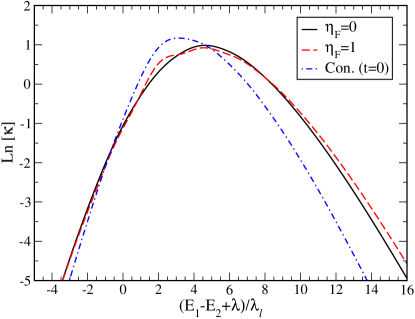
Figure 1 shows results for Case I of Table 2, for which there is no high frequency component of the spectral densities (thus ) and the temperature is high enough for the bath to be viewed as being almost classical. Rates calculated by Eq. (51) for and are shown. As a reference, rate calculated according to the following Condon approximation is also shown.
| (70) |
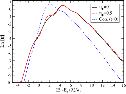
which employs the NDC terms at for the calculation of an effective coupling. This choice of reference rate remains the same for the figures that follow. When compared to this approximation, it is clear that the contribution of enhances the rate preferentially for larger values of . The resulting shape of the rate vs. energy becomes slightly more asymmetric, but it appears that the whole behavior can still be modeled reasonably well by a Condon-type rate expression if an effective modification of can be made. Comparison of the result for with that for shows that the former enhances the rate for only large value of . On the other hand, for , interesting crossing appears between the two rates.
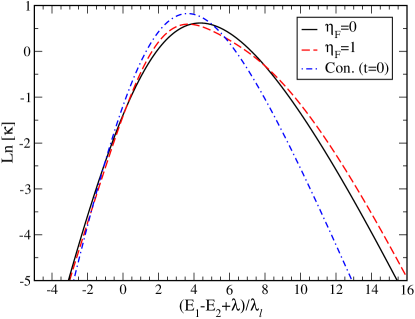
Figure 2 provides results for Case II of Table 2, for which the energy of the high frequency vibrational mode is much larger than thermal energy and the cutoff frequency of the Ohmic bath. As yet, due to the dominance of the low frequency Ohmic bath, the effects of the high frequency vibrational mode are relatively minor in this case. Thus, the results are qualitatively similar to those for Fig. 1.
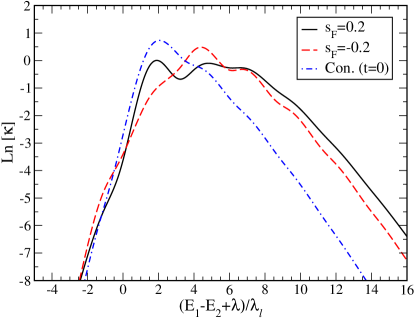
Calculation results for the same Case II of Table 2 but now with finite value of are presented in Fig. 3. Note that the result is independent of the overall sign of . On the other hand, the relative sign of the Ohmic bath and the high frequency vibrational component makes difference because different relative signs result in different net contribution to . For larger value of , the case with results in larger rate compared to the case with . However for small or moderately negative values of , opposite situations can occur, which can be due to subtle interplay of oscillatory nature of integrands.
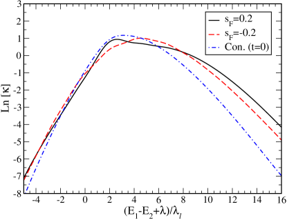
Figure 4 shows results for Case III of Table 2, for which there is no high frequency component of the spectral densities (thus ) but the temperature is low compared to the width of the Ohmic spectral density. As a result, clear asymmetry can be seen even for the approximate result with Condon approximation, Eq. (70), indicating that the bath has significant quantum mechanical character. Since there is no high frequency vibrational mode in this case, resulting rates have similar trends as in Fig. 1.
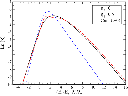
Figure 5 provides results for Case IV of Table 2, for which there is a contribution of a high frequency vibrational mode to both and . The energy quantum of the high frequency vibrational mode relative to the thermal energy is the same as Case II, and the resulting rate even for the Condon approximation exhibits a slight oscillatory pattern. It is seen that the contribution of the low frequency Ohmic bath to causes significant shift of the rate, when compared to that of Condon approximation, and also makes the vibrational progression more pronounced in the normal region (negative values of ). On the other hand, additional contribution of the low frequency Ohmic bath to does not seem to bring significant changes. Even for large values of , the enhancement of the rate due to the finite value of is rather minor.
Finally, results for Case IV of Table 2 but now in the presence of contributions of both the low frequency Ohmic bath and the high frequency vibrational mode to are shown in Fig. 6. The effects of the high frequency component and its relative sign are shown to have significant effects. The results for positive value of are shown to enhance the rate consistently for large value of , but there are two regions where the negative value of produce higher rates. Overall, the rates are shown to be sensitive to both magnitude and sign of for values of comparable to . These results indicate the importance of accurate and detailed characterization of the nature of NDC terms to vibrational modes for quantitative modeling of rates.
V Conclusion
Starting from a general expression for the molecular Hamiltonian in the adiabatic electronic states and nuclear position states, we have considered NDC terms carefully and clarified issues that make straightforward application of FGR for nonadiabatic transitions difficult. We then derived a general expression for the FGR rate under a quasiadiabatic approximation, which employs crude adiabatic electronic states determined at the minimum of the initial adiabatic electronic state. For the case where all the nuclear dynamics are modeled as displaced harmonic oscillators, we then derived an explicit expression for the FGR rate. The resulting rate expression, Eq. (51), explicitly accounts for non-Condon effects due to momentum terms, and thus can be used for more accurate calculation of nonradiative rates beyond Condon approximation.
We have conducted model calculations for cases where the spectral density consists of a low frequency Ohmic bath (with an exponential cutoff) and a single high frequency vibrational mode. Results of calculation for sets of parameters in Table 2, with additional choice of parameters for , demonstrate nontrivial non-Condon effects due to NDC terms. For the bath spectral density consisting only of the Ohmic bath, effects of NDC terms do not seem to result in significant qualitative changes in the dependence of the rate on the energy gap. It is likely that the general behavior can still be captured well by an effective Condon-like rate expression.
On the other hand, with additional contribution of a high frequency vibrational mode, the non-Condon contribution of the NDC term and its detailed manner of coupling (including relative sign) with the Franck-Condon modes and the value of the energy have intricate contributions to the rate. Nonetheless, there is consistent enhancement of rate due to NDC terms for significantly larger energy gap between the donor and acceptor in general.
Results of the present paper offer new insights into rate processes due NDC terms such as nonradiative decay of near infrared and short-wave infrared dye moleculesFriedman et al. (2021); Erker and Basche (2022) that follow the energy gap law.Englman and Jortner (1970); Jang (2021) A recent workRamos et al. (2024) demonstrated the importance of NDC terms projected onto all vibrational frequencies of molecules, but the detailed contribution of non-Condon effects has not been clarified yet. New theoretical expressions and model calculations provided here will help determine such effects quantitatively along with additional computational data needed to characterize all the relevant spectral densities.
Acknowledgements.
S.J.J. acknowledges primary support from the US Department of Energy, Office of Sciences, Office of Basic Energy Sciences (DE-SC0021413) and partial support during the initial stage of this project from the National Science Foundation (CHE-1900170). Y.M.R. acknowledges support from the National Research Foundation (NRF) of Korea (Grant No. 2020R1A5A1019141). This project initiated during sabbatical stay of S.J.J. at Korea Advanced Institute of Science and Technology (KAIST) and Korea Institute for Advanced Study (KIAS). S.J.J. thanks support from the KAIX program at KAIST and KIAS Scholar program for the support of sabbatical visit.Appendix A Normal mode representation and harmonic approximation
Expanding the potential energy , which appears in Eq. (28), around with respect to up to the second order and diagonalizing the resulting Hessian matrix, one can determine all of normal vibrational modes and frequencies, and with , where is the total number of normal mode vibrations for the vibrational motion around in the electronic state 1. The transformation from Cartesian coordinates to these normal modes are defined as follows:
| (71) | |||||
Then, assuming that all the vibrational modes have small enough amplitudes such that quadratic approximation of the potential energy remains reliable and that an Eckart frame that fully decouples the rotational and vibrational degrees of freedom can be found, the nuclear Hamiltonian operator in Eq. (28) can be approximated as
| (72) |
where is the canonical momentum operator for and represents the translation of the center-of-mass and rotational motion around . For the calculation of the FGR rate for electronic transition from isolated molecule, it is reasonable to assume that this can be neglected considering the disparity between typical electronic transition energies and nuclear translation-rotation energies.
In a similar manner, the potential energy in Eq. (28) can be expanded around its minimum energy structure position . However, in such expansion, it is important to recognize first that is already defined in the Eckart frame with respect to , which does not in general satisfy the second Eckart conditionLouck and Galbraith (1976) for . This has the following two consequences:
- 1.
-
2.
Purely vibrational displacement from may bear some rotational component around .
At the moment, complete resolution of the above two issues seems not possible in general. While these issues may be mitigated by adopting curvilinear internal coordinates, whether it results in actual advantage is not clear.Min et al. (2023) Thus, we use Cartesian coordinates and invoke additional assumptions here. First, we assume that the non-uniquenessLouck and Galbraith (1976); Dymarsky and Kudin (2005) in the choice of the Eckart frame for can be utilized such that is maximally aligned with . This will minimize the coupling term between the rotation and vibration parts for the displacement around , which we assume to be small enough and can thus can be ignored. Similarly, we assume that the projection of pure vibrational components around onto rotational part around can be discarded.
With approximations and assumptions as noted above, which can always be tested for a given molecular system, we can expand with respect to around and identify the normal mode and frequency, and , for , where is the total number of normal mode vibrations for the vibrational motion around . These are related to mass-weighted cartesian coordinates in the best Eckart frame, as noted above, by the following transformation,
Thus, we can make the following approximation:
| (74) |
In the above expression, represents the translation of the center-of-mass and rotational motion around , which is assumed to be negligible for the calculation of the electronic transition rate.
Appendix B Expression for the coupling Hamiltonian with respect to normal mode coordinates
Let us consider the following matrix element:
| (75) |
We assume that all the translation and rotational degrees of freedom are frozen. Then,
| (76) | |||||
Therefore,
| (77) | |||||
Similarly, defined by Eq. (29) can be expressed in terms of given by Eq. (34) as follows:
| (78) |
As a result, we find that
| (79) |
Since the above identity holds for an arbitrary vector , which does not have any translation and rotational degree, and for any state , this proves the first equality of Eq. (LABEL:eq:hc-2).
Appendix C Calculation of bath correlation functions
Consider the following harmonic oscillator bath Hamiltonian and a bath term linear in position:
| (80) | |||
| (81) |
For the equilibrium density , let us first consider the following well-known time correlation function:
| (82) |
Then, using with ,
| (83) | |||||
where and
| (84) |
The trace in Eq. (83) can be evaluated as follows:
| (85) |
where
| (86) |
Therefore,
| (87) |
Now, consider the following time correlation function:
| (88) |
Following a procedure similar to Eq. (83), we find that
| (89) | |||||
Note that is proportional to as follows:
| (90) |
Therefore, the trace operation in Eq. (89) can be expressed as
| (91) |
Following a procedure similar to obtaining Eq. (85), we can calculate the trace in the above expression as follows:
| (92) |
Therefore,
| (93) |
Second, let us consider the following time correlation function:
| (94) |
Following a procedure similar to Eq. (83), we find that
| (95) | |||||
Employing Eq. (90) for , we find that the trace in the last line of the above equation can be expressed as
| (96) |
The trace in the above expression can be calculated in a way similar to Eq. (92) as follows:
| (97) |
Therefore,
| (98) |
Finally, let us consider the following momentum correlation function:
| (99) | |||||
Following a procedure similar to Eq. (83), we find that
| (100) | |||||
In the above expression, the trace can be expressed as
| (101) |
Following a procedure similar to Eqs. (92) and (97), the trace in the above expression can be calculated as follows:
Taking partial derivatives of the above expression with respect to and , we find that
where is defined by Eq. (86). Employing the above expression in Eq. (101) and then using Eq. (100), we obtain the following expression:
| (104) | |||||
References
- Makhov et al. (2017) D. V. Makhov, C. Symonds, S. Fernandez-Alberti, and D. V. Shalashilin, “Ab initio quantum direct dynamics simulations of ultrafast photochemistry with multiconfigurational ehrenfest approach,” Chem. Phys. 493, 200–218 (2017).
- Tao, Levine, and Martinez (2009) H. L. Tao, B. G. Levine, and T. J. Martinez, “Ab initio multiple spawning dynamics using mult-state second-order perturbation theory,” J. Phys. Chem. A 113, 13656 (2009).
- Goings, Lestrange, and Li (2017) J. J. Goings, P. L. Lestrange, and X. Li, “Real-time time-dependent electronic structure theory,” WIREs Comput. Mol. Sci. , e1341 (2017).
- Wang, Long, and Prezhdo (2015) L. Wang, R. Long, and O. V. Prezhdo, “Time domain ab initio modeling of photoinduced dynamics at nanoscale interfaces,” Annu. Rev. Phys. Chem. 66, 549–579 (2015).
- Curchod and Martinez (2018) B. F. E. Curchod and T. J. Martinez, “Ab initio nonadiabatic quantum molecular dynamics,” Chem. Rev. 118, 3305–3336 (2018).
- Guo, Worth, and Domcke (2021) H. Guo, G. Worth, and W. Domcke, “Quantum dynamics with ab initio potentials,” J. Chem. Phys. 155, 080401 (2021).
- Zhao et al. (2020) L. Zhao, Z. Tao, F. Pavosevic, A. Wildman, S. Hammes-Schiffer, and X. Li, “Real-time time-dependent nuclear-electronic orbital approach: Dynamics beyond the born-oppenheimer approximation,” J. Phys. Chem. Lett. 11, 4052–4058 (2020).
- Song et al. (2020) H. Song, S. A. Fischer, Y. Zhang, C. J. Cramer, S. Mukamel, N. Govind, and S. Tretiak, “First principles nonadiabatic excited-state molecular dynamics in nwchem,” J. Chem. Theory Comput. 16, 6418–6427 (2020).
- Hegger, Binder, and Burghardt (2020) R. Hegger, R. Binder, and I. Burghardt, “First-principles quantum and quantum-classical simulations of exciton diffusion in semiconducting polymer chains at finite temperature,” J. Chem. Theory Comput. 16, 5441–5455 (2020).
- Gao and Rossky (2022) J. Gao and P. J. Rossky, “The age of direct chemical dynamics,” Acc. Chem. Res. 55, 471–472 (2022).
- Tully (2012) J. C. Tully, “Perspective: Nonadiabatic dynamics theory,” J. Chem. Phys. 137, 22A301 (2012).
- Jasper et al. (2006) A. W. Jasper, S. Nangia, C. Zhu, and D. G. Truhlar, “Non-born-oppenheimer molecular dynamics,” Acc. Chem. Res. 39, 101–108 (2006).
- A. F. Izmaylov, D. Mendive-Tapia, M. J. Bearpark, M. A. Robb, J. C. Tully, and M. J. Frisch (2011) A. F. Izmaylov, D. Mendive-Tapia, M. J. Bearpark, M. A. Robb, J. C. Tully, and M. J. Frisch, “Nonequilibrium fermi golden rule for electronic transitions through conical intersection,” J. Chem. Phys. 135, 234106 (2011).
- Kapral (2006) R. Kapral, “Progress in the theory of mixed quantum-classical dynamics,” Annu. Rev. Chem. Phys. 57, 129–157 (2006).
- Subotnik et al. (2016) J. E. Subotnik, A. Jain, B. Landry, A. Petit, W. Ouyang, and N. Bellonzi, “Understanding the surface hopping view of electronic transitions and decoherence,” Annu. Rev. Phys. Chem. 67, 387–417 (2016).
- Esch and Levine (2021) M. P. Esch and B. G. Levine, “An accurate, non-empirical method for incorporating decoherence into ehrenfest dynamics,” J. Chem. Phys. 155, 214101 (2021).
- Huang, Green, and Martens (2023) D. M. Huang, A. T. Green, and C. C. Martens, “A first principles derivation of energy-conserving momentum jumps in surface hopping simulations,” J. Chem. Phys. 159, 214108 (2023).
- Zhu and Yarkony (2005) X. Zhu and D. R. Yarkony, “Quasi-diabatic representations of adiabatic potential energy surfaces coupled by conical intersections including bond breaking: A more general construction procedure and an analysis of the diabatic representation,” J. Chem. Phys. 1, 22A511 (2005).
- Joubert-Doriol and Izmaylov (2018) L. Joubert-Doriol and A. Izmaylov, J. Phys. Chem. A 122, 6031–6042 (2018).
- Xhou, Mandal, and Huo (2019) W. Xhou, A. Mandal, and P. Huo, “Quasi-diabatic scheme for nonadiabatic on-the-fly simulations,” J. Phys. Chem. Lett. 10, 7062–7070 (2019).
- Prezhdo (2021) O. V. Prezhdo, “Modeling non-adiabatic dynamics in nanoscale and condensed matter systems,” Acc. Chem. Res. 54, 4329–4249 (2021).
- Shu et al. (2022) Y. Shu, L. Zhang, X. Chen, S. Sun, Y. Huang, and D. G. Truhlar, “Nonadiabatic dynamics algorithms with only potential energies and gradients: Curvature-driven coherent switching with decay of mixing and curvature-driven trajectory surface hopping,” J. Chem. Theory Comput. 18, 1320–1328 (2022).
- Knox (1963) R. S. Knox, Theory of excitons (Academic Press, New York, 1963).
- Kenkre and Reineker (1982) V. M. Kenkre and P. Reineker, Exciton Dynamics in Molecular Crystals and Aggregates (Springer, Berlin, 1982).
- May and Kühn (2011) V. May and O. Kühn, Charge and Energy Transfer Dynamics in Molecular Systems (Wiley-VCH, Weinheim, Germany, 2011).
- Jang (2020) S. J. Jang, Dynamics of Molecular Excitons (Nanophotonics Series) (Elsevier, Amsterdam, 2020).
- Lin (1973) S. H. Lin, “Radiationless transitions in isolated molecules,” J. Chem. Phys. 58, 5760–5768 (1973).
- Mebel et al. (1999) A. M. Mebel, M. Hayashi, K. K. Liang, and S. H. Lin, “Ab initio calculations of vibronic spectra and dynamics for small polyatomic molecules: Role of duschinsky effect,” J. Phys. Chem. A 103, 10674–10690 (1999).
- Niu, Peng, and Shuai (2008) Y. Niu, Q. Peng, and Z. Shuai, “Promoting-mode free formalism for excited state radiationless decay process with duschinsky rotation effect,” Sci. China Ser. B-Chem. 51, 1153–1158 (2008).
- Niu et al. (2010) Y. Niu, Q. Peng, C. Deng, X. Gao, and Z. Shuai, “Theory of excited state decays and optical spectra: Application to polyatomic molecules,” J. Phys. Chem. A 114, 7817–7831 (2010).
- Wang, Ren, and Shuai (2021) Y. Wang, J. Ren, and Z. Shuai, “Evaluating the anharmonicity contributions to the molecular excited internal conversion rates with finite temperature td-dmrg,” J. Chem. Phys. 154, 214109 (2021).
- Borrelli and Peluso (2008) R. Borrelli and A. Peluso, “Perturbative calculation of franck-condon integrals: New hints for a rational implementation,” J. Chem. Phys. 129, 064116 (2008).
- Jang (2012) S. Jang, “Nonadiabatic quantum liouville equation and master equations in the adiabatic basis,” J. Chem. Phys. 137, 22A536 (2012).
- Note (1) This assumption will be relaxed later once adiabatic basis of molecular states are identified.
- Jang (2023) S. J. Jang, Quantum Mechanics for Chemistry (Springer Nature, New York, 2023).
- Note (2) The original notations were slightly altered and was incorporated into derivative coupling terms in this work.
- Hellmann (1993) H. Hellmann, Einführung in die Quantrnchemie (Franz Deuticke, Leipzig, 1993).
- Feynman (1939) R. P. Feynman, “Forces in molecules,” Phys. Rev. 56, 340–343 (1939).
- Note (3) More precisely stated, this implies that there are two adiabatic electronic state surfaces constructed by joining those for fixed nuclear coordinates s.
- Eckert (1935) C. Eckert, “Some studies concerning rotating axes and polyatomic molecules,” Phys. Rev. 47, 552–558 (1935).
- Louck and Galbraith (1976) J. D. Louck and H. W. Galbraith, “Eckart vectors, eckart frames, and polyatomic molecules,” Rerv. Mod. Phys. 48, 69–106 (1976).
- Pickett and Strauss (1970) H. M. Pickett and H. L. Strauss, “Conformational structure, energy, and inversion rates of cyclohexane and some related oxanes,” J. Am. Chem. Soc. 92, 7281–7290 (1970).
- Dymarsky and Kudin (2005) A. Y. Dymarsky and K. N. Kudin, “Computation of the pseudorotation matrix to satisfy the eckart axis conditions,” J. Chem. Phys. 122, 124103 (2005).
- Jang and Rhee (2023) S. J. Jang and Y. M. Rhee, “Modified fermi’s golden rule rate expressions,” J. Chem. Phys. 159, 014101 (2023).
- Friedman et al. (2021) H. C. Friedman, E. D. Cosco, T. L. Atallah, S. Jia, E. M. Sletten, and J. R. Caram, “Establishing design principles for emissive organic swir chromophores from energy gap laws,” Chem 7, 1–18 (2021).
- Erker and Basche (2022) C. Erker and T. Basche, “The energy gap law at work: Emission yield and rate fluctuations of single nir emitters,” J. Am. Chem. Soc. 144, 14053–14056 (2022).
- Englman and Jortner (1970) R. Englman and J. Jortner, “The energy gap law for radationless transitions in large molecules,” Mol. Phys. 18, 145–164 (1970).
- Jang (2021) S. J. Jang, “A simple generalization of the energy gap law for nonradiative processes,” J. Chem. Phys. 155, 164106 (2021).
- Ramos et al. (2024) P. Ramos, H. Friedman, B. Y. Li, C. Garcia, E. Sletten, J. R. Caram, and S. J. Jang, “Nonadiabatic derivative couplings through multiple franck-condon modes dictate the energy gap law for near and short-wave infrared dye molecules,” J. Phys. Chem. Lett. 15, 1802–1810 (2024).
- Min et al. (2023) B. K. Min, D. Kim, D. Kim, and Y. M. Rhee, Bull. Kor. Chem. Soc. 44, 989–1003 (2023).