Semi-supervised Symmetric Matrix Factorization with Low-Rank Tensor Representation
Abstract
Semi-supervised symmetric non-negative matrix factorization (SNMF) utilizes the available supervisory information (usually in the form of pairwise constraints) to improve the clustering ability of SNMF. The previous methods introduce the pairwise constraints from the local perspective, i.e., they either directly refine the similarity matrix element-wisely or restrain the distance of the decomposed vectors in pairs according to the pairwise constraints, which overlook the global perspective, i.e., in the ideal case, the pairwise constraint matrix and the ideal similarity matrix possess the same low-rank structure. To this end, we first propose a novel semi-supervised SNMF model by seeking low-rank representation for the tensor synthesized by the pairwise constraint matrix and a similarity matrix obtained by the product of the embedding matrix and its transpose, which could strengthen those two matrices simultaneously from a global perspective. We then propose an enhanced SNMF model, making the embedding matrix tailored to the above tensor low-rank representation. We finally refine the similarity matrix by the strengthened pairwise constraints. We repeat the above steps to continuously boost the similarity matrix and pairwise constraint matrix, leading to a high-quality embedding matrix. Extensive experiments substantiate the superiority of our method. The code is available at https://github.com/JinaLeejnl/TSNMF.
Index Terms:
Symmetric non-negative matrix factorization, tensor low-rank representation, semi-supervised clustering.I Introduction
Symmetric non-negative matrix factorization (SNMF) [4] takes a non-negative matrix as input, and decomposes it as the product of two identical non-negative matrices, i.e.,
| (1) |
where is the embedding matrix, means each element of is no less than zero, and and indicate the number of the samples and the feature dimension of the embedding matrix. When denotes a similarity matrix of a group of samples, SNMF becomes a well-known graph clustering method [3]. For a typical graph clustering method like spectral clustering (SC) [4], [31], an embedding matrix is first generated and then a post processing like -means [27] is required to be performed on the embedding matrix to get the final clustering result. Different from SC, SNMF can directly generate the clustering results utilizing the calculated embedding matrix owning to the non-negative constraints on [3]. Due to this favorable point, SNMF has been applied to many applications like pattern clustering in gene expression [28], community detection [29], multi-document summarization [30], etc. Many variants have also emerged based on SNMF. For instance, Luo et al. [14] proposed pointwise-mutual-information-incorporated and graph-regularized SNMF (PGSNMF). By implementing SNMF while preserving the geometrical information of the data, Gao et al. [15] proposed graph regularized SNMF (GrSNMF).
Many applications in the real world have a small amount of supervisory information available. For example, in the video face clustering, two faces in the same video frame cannot belong to the same person [32]. Those supervisory information can be generally transformed into two kinds of pairwise constraints, i.e., must-link (ML) and cannot-link (CL), which respectively indicate two data samples belong to the same class or just the opposite. Incorporating those supervisory information can improve the clustering ability of SNMF, which is known as semi-supervised SNMF [7]. Recently, many semi-supervised SNMF methods were proposed. For example, Yang et al. [8] proposed to introduce MLs through a graph Laplacian regularization, hoping the embeddings of two samples with an ML to be close to each other. Zhang et al. [9] proposed SNMF based constrained clustering (SNMFCC), which restricts the inner product of the embeddings of two samples with an ML to be large while that with a CL to be small. By simultaneously completing embedding learning and similarity matrix construction, Wu et al. [10] proposed pairwise constraint propagation-induced SNMF (PCPSNMF). Qin et al. [11] added an additional sparse regularizer and an additional smoothness regularizer on PCPSNMF. Jia et al. [12] proposed the semi-supervised adaptive SNMF (SANMF) to emphasize CLs. See Section II for details on these algorithms.
Existing semi-supervised SNMF methods introduce the supervisory information from a local perspective. For example, in [8] and [9], if there exists an ML (resp. a CL) between the -th and the -th samples, their embeddings and are enforced to be similar (resp. dissimilar) to each other. In [10, 11, 12], they adjust the value of the similarity matrix according to the pairwise constraints, i.e., the similarity should be large for two samples with an ML and small for those with a CL. As these methods incorporate the pairwise constraints locally, i.e., element-wisely or sample-to-sample pair-wisely, we argue the global relationship between the pairwise constraints and the embedding matrix is ignored, which leads to inadequate utilization of supervisory information.
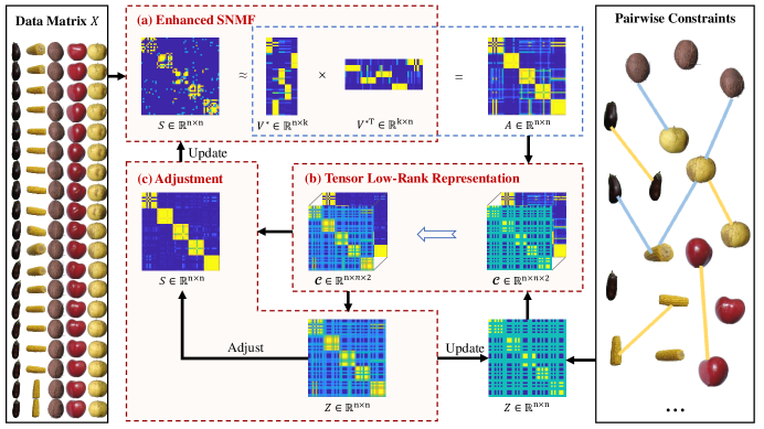
We observe that when all the pairwise constraints are available, the pairwise constraint matrix is a binary block-diagonal matrix with size . At the same time, the ideal embedding matrix is a binary matrix. Specifically, each row only has one element equaling to 1 whose column index suggests the clustering membership, while others equaling to 0. Moreover, the product of the embedding matrix with its transpose becomes a similarity matrix owing the same block-diagonal structure as the ideal pairwise constraint matrix. So we stack them into a 3-dimensional (3D) tensor and as the two slices of the tensor share the same block-diagonal structure, we could impose a global prior like tensor low-rank norm to capture the global relationship between the pairwise constraint matrix and the embedding matrix. By applying the tensor low-rank representation, more pairwise constraints can be interfered by exploring the information from the embedding matrix, and at the same time, the embedding matrix can also be promoted by the available supervisory information. Unfortunately, applying a low-rank prior on the formed tensor directly is ineffective as the similarity matrix composed by the embedding matrix is already low-rank, i.e., rank() rank() and is generally much greater than . To this end, we propose an enhanced SNMF to make the learned embedding matrix have a larger rank to be tailored to the tensor low-rank prior. The proposed enhanced SNMF has the same input as the traditional SNMF but is more robust to initialization. After obtaining the embedding matrix by the enhanced SNMF, we apply the tensor low-rank norm on the formed 3D tensor, and then we refine the input similarity matrix by the promoted pairwise constraint matrix. These three steps are performed alternatively and iteratively. The overall framework is shown in Fig. 1. We compare the proposed method with 9 state-of-the-art (SOTA) methods on 6 datasets. Experiments show that our proposed model is superior to the SOTA methods.
Our work’s contributions are summarized as follows:
-
•
We exploit the supervisory information from a global perspective by constructing a 3D tensor and imposing the tensor low-rank representation on it, which could concurrently promote the pairwise constraints and the input similarity matrix.
-
•
We propose an enhanced version of SNMF tailored to the tensor low-rank representation. It can produce a higher-quality and more stable embedding matrix with better clustering performance compared to SNMF.
-
•
We conduct a series of experiments to prove the robustness and effectiveness of our method.
The remainder of the paper is organized as follows. We briefly review some related works in Section II. In Section III, we detail the proposed method, and in Section IV, we introduce how to optimize the method. In Section V we carry out extensive experiments to compare the proposed method with the SOTA methods. Section VI concludes the paper. For convenience, the symbols used in the rest of this paper are summarized in Table I.
| Symbol | Meaning |
| input space | |
| original feature space | |
| embedding feature space | |
| tensor (bold calligraphy letter) | |
| matrix (regular uppercase letter) | |
| vector (bold lowercase letter) | |
| scalar (regular lowercase letter) | |
| sample | |
| set of ’s | |
| symmetric weight matrix | |
| , | embedding matrix |
| similarity among samples, i.e., | |
| pairwise constraint matrix | |
| Frobenius norm (the open root of the sum of the squares of all the elements of a matrix) | |
| nuclear norm (the sum of the singular values of a matrix, and for a tensor, there are various different definitions. In this paper, we used the tensor nuclear norm defined in [25]) |
II Related Work
Given a sample matrix , which means there are samples in the -dimensional space. is a symmetric weight matrix, where represents the similarity between sample and . Typically, we can construct the weights according to the algorithm [10], i.e.,
| (2) |
where represents that two samples are the nearest neighbors of each other, and is a hyper-parameter. In this paper, we set as the average distance from a point to its nearest neighbors. We use matrix to represent available constraints:
| (3) |
II-A NMF and Symmetric NMF
Given a non-negative matrix , NMF [1], [2] approximately decomposes it into the product of two smaller non-negative matrices and , that is, . NMF usually uses the Euclidean distance to measure the closeness between input and its approximated decomposition, leading to the following cost function:
| (4) |
represents the -dimensional basis matrix, represents the embedding matrix (a.k.a. coefficient matrix), and and constrain each element in and to be non-negative, that is, only additive operations exist in NMF. In addition, NMF can be regarded as a clustering method [5], which is widely used in tasks such as consensus clustering [16] and community detection [17].
NMF is not suitable for data with nonlinear cluster structures, while SNMF can better separate the data with nonlinear cluster structure. Unlike NMF, which takes the original data matrix as input, the input of SNMF is a similarity matrix , whose elements reflect the relationship between data points. Specifically, SNMF decomposes into the product of a non-negative matrix and its transpose, i.e.,
| (5) |
As is non-negative, the column index of the largest entry in each row of can directly indicate the cluster membership of a sample. Due to this favorable characteristic, SNMF is widely used in many clustering tasks such as signal and data analytics [18], biomedicine [19], semantic analysis of documents [30], etc.
II-B Semi-supervised SNMF
Recently, many variants of SNMF were proposed to incorporate the supervisory information, which is known as the semi-supervised SNMF. For example, Yang et al. [8] proposed GSNMF by integrating the must-links, i.e.,
| (6) |
where represents the th row of and is defined as:
| (7) |
By minimizing Eq. (6), two samples connected by an ML will have the similar embeddings. To incorporate both MLs and CLs, Zhang et al. [9] proposed SNMFCC, i.e.,
| (8) |
where means the element-wise Hadamard product. is defined as:
| (9) |
where and are hyper-parameters, representing the importance of ML and CL respectively. SNMFCC effectively integrates both ML and CL by employing Eq. (8), ensuring that the product of the embedding matrix and its transpose reflects the pairwise constraints.
In order to ameliorate the predefined similarity matrix by the pairwise constraints, Wu et al. [10] proposed PCPSNMF, whose formula is as follows:
| (10) |
where is a graph Laplacian matrix. constructs a symmetric similarity matrix, and are hyper-parameters. Eq. (10) simultaneously updates the similarity matrix and the embedding matrix.
Realizing the ideal similarity matrix owns the block-diagonal structure, Qin et al. [11] proposed S3NMF by adding an additional sparsity promoting term on the loss function of PCPSNMF, i.e.,
| (11) |
where is the -norm (the sum of the absolute values of all elements of a matrix). and are hyper-parameters, and is used to introduce the sparsity promoting term. In order to make CLs play a greater role, Jia et al. [12] proposed SANMF:
| (12) |
SANMF introduced CL propagation to distinguish CLs from unknown pairwise relations and to assist the propagation of MLs.
III Proposed Model
III-A Motivation
Although the existing semi-supervised SNMF methods have produced remarkable clustering performance, they all incorporate the pairwise constraints from a local perspective. Specifically, they either constrain the distance between the embeddings of two samples with an ML or a CL like GSNMF and SNMFCC, or they refine the input similarity matrix element-wisely according to the pairwise constraints like PCPSNMF and SANMF. However, all of them do not consider global structure of the pairwise constraint matrix. In the ideal case, the pairwise constraint matrix is a binary block-diagonal matrix if all the samples are aligned by the class membership. Moreover, the ideal similarity matrix shares the same global structure as the ideal pairwise constraint matrix. Motivated by this observation, we aim to include the pairwise constraints from the global perspective.
III-B Incorporate the Pairwise Constraints by Tensor Low-Rank Representation
Let represent the embedding matrix. The product between and its transpose can indicate the similarity among samples as is non-negative. Moreover, in the ideal case, the composed is also a binary block-diagonal matrix, i.e., if and belong to the same cluster and if and belong to different clusters [20]. That means the ideal pairwise constraint matrix and the ideal similarity matrix share the same block-diagonal structure. To capture this global prior, we propose to stack the matrix and the pairwise constraint matrix into a 3D tensor, and impose a tensor low-rank prior on the build tensor. By pursuing the tensor low-rank representation, the similarity matrix can be ameliorated by the available pairwise constraints while the initial pairwise is also boosted by the similarity matrix, i.e., more pairwise constraints can be inferred. Such a self-boosting strategy constantly improve both the pairwise constraint matrix and the similarity matrix, which is mathematically formulated as
| (13) |
where represents the pairwise constraint matrix, represents the refined similarity matrix, denotes the 3D tensor stacked by (the first slice) and (the second slice). represents the initial similarity matrix. For the refined similarity matrix , we hope it is well aligned with pairwise constraints such that it can be improved by the supervisory information. Moreover, it should be close to the initial similarity matrix , as the information in the is also valuable. Therefore, we assume that , where denotes the error between and , and we minimize the Frobenius norm of . For the pairwise constraint matrix , we initialize it with available supervisory information and hope that more pairwise constraints are inferred to enhance . Finally, we apply nuclear norm defined in [25] to obtain the low-rank representation. Other tensor low-rank norms are also applicable here. Note that this self-boosting strategy in Eq. (13) is achieved by the global relationship between the two slices of the 3D tensor through the tensor low-rank representation, which is quite different from the previous local perspective.
However, directly using the generated by SNMF cannot achieve the above target, since rank() rank() and is generally much greater than , the rank of is very small, and low-rank constraint on the tensor will lose the designed effect. Therefore, we propose an Enhanced SNMF to solve this problem.
III-C Enhanced SNMF
To make the embedding of the SNMF fit the tensor low-rank representation in Eq. (13), we propose an enhanced SNMF that can produce an embedding with a larger rank only using the same input as the traditional SNMF. Specifically, given a similarity matrix , we first decompose it into a set of embedding matrices , where denotes the number of embeddings. Then, we construct a high-quality embedding matrix as the final result by weighting the embedding matrices set with an adaptive weight vector . The proposed enhanced SNMF incorporates the above steps into a joint optimization model, i.e.,
| (14) |
where denotes the weight vector, and is to ensure the validity of the weight value. We generate a set of embedding matrices from the same input similarity matrix by minimizing . To guarantee the diversity of , we can simply initialize them with different initializations as SNMF is quite sensitive to the initialization [21]. Then we obtain the final embedding through to make be consistent with . Different from with a fixed rank, the constructed consistent embedding usually has a larger rank. Moreover, different initializations will lead to diverse , but the embedding qualities of are also varied. To keep a high-quality embedding, we introduce a weight vector to measure the quality of each . Specifically, if is superior in quality, the residual error is supposed to be small (i.e., is small), and the corresponding weight should be large, otherwise should be small. We achieve this goal by . The constraints on (i.e., and ) makes a well-defined weight vector. We also impose a regularization term on () to avoid the trivial solution that only one element of is and the remaining elements are . The learned can be used to adjust the contribution of each to the construction of by minimizing , i.e., a higher quality will contribute more in the learning of .
As a summary, by solving the problem in Eq. (14), we get an embedding with higher rank that is tailored to low-rank representation problem in Eq. (13). Moreover, the enhanced SNMF has the same input as the traditional SNMF but with improved robustness as it integrates different embeddings together with an adaptive weighting strategy.
III-D Similarity Matrix Refinement by the Enhanced Pairwise Constraints
After solving Eq. (13), we obtain an enhanced pairwise constraint matrix and a promoted similarity matrix , then we propose to further use the enhanced pairwise constraint matrix to adjust the similarity matrix promoted by Eq. (13). Specifically, for a positive element in , it is likely to be an ML, we, therefore, increase the weight of the corresponding element in the similarity matrix. And for the same reason, we decrease the weight of the similarity matrix for a negative element in . The adjustment strategy is formulated as
| (15) |
IV Optimization
IV-A Overall Optimization Method
For better clustering performance, we first use the pairwise constraint matrix to adjust the similarity matrix through Eq. (15). Then, we input the preprocessed into Eq. (14), and obtain the initial embedding matrix by the Enhanced SNMF. Finally, we utilize Eq. (13) to simultaneously improve and the pairwise constraint matrix . The above steps are regarded as an iteration, and the optimized can be used as the input of the next iteration. Repeated iterations can make the similarity matrix and pairwise constraint matrix keep getting better. See Algorithm 1 for details.
IV-B Algorithm for Solving the Enhanced SNMF in Eq. (14)
Eq. (14) is non-convex with multiple variables. It is difficult to find the global minimum, so we use an alternative method to find a local minimum, that is, first update with fixed and , then update with fixed and , and finally update with fixed and . Eq. (14) can be expressed as the following loss function:
| (16) |
where means the trace of a matrix, i.e., the sum of the elements on the main diagonal of the matrix.
The embedding matrices are independent of each other, so we solve each -problem separately. After removing the items irrelevant to in Eq. (16), the Lagrange equation about can be expressed as follows:
| (17) |
where is the Lagrangian multiplier matrix. Taking the first order derivative of Eq. (17) with respect to , we have
| (18) |
Let , can be updated by
| (19) |
where represents the number of iterations. In the same way, the first derivative of Eq. (16) with respect to is
| (20) |
Then we update by , i.e.,
| (21) |
The sub-problem of Eq. (16) about can be written as:
| (22) |
where and . This is a problem of computing the Euclidean projection of a point onto the capped simplex, which can be addressed by [22]. Algorithm 2 shows the specific process of solving Eq. (14).
IV-C Algorithm for Solving Eq. (13)
We solve Eq. (13) by the alternating direction method of multipliers (ADMM), which is very effective for solving problems with multiple variables and equality constraints [23], [24]. We first introduce an auxiliary matrix , and let , then Eq. (13) can be written as:
| (23) |
The augmented Lagrangian function of Eq. (23) can be expressed as:
| (24) |
Among them, , , and are the Lagrangian multipliers corresponding to , , and respectively, is the Lagrangian multiplier matrix, and is the augmented Lagrangian coefficient. We also adopt an alternative iterative method to solve Eq. (24). Specifically, the sub-problem with respect to can be written as follows:
| (25) |
It has a closed-form solution by the tensor Singular Value Thresholding (t-SVT) operator [25], i.e.,
| (26) |
where is the t-SVT operator, , .
Calculate the first-order derivative of for Eq. (24):
| (27) |
Let , we get the alternate iteration formula of :
| (28) |
The first order derivative of Eq. (24) with respect to is:
| (29) |
Since , we set and get the update formula for as follows:
| (30) |
In Eq. (30), we divide a matrix into positive and negative parts [26], which are calculated as follows:
| (31) |
In the same way, after calculating the first-order derivative of in Eq. (24), let the first-order derivative function be 0, and the update rule of can be obtained as follows:
| (32) |
The solution to the subproblem of is:
| (33) |
In addition, the update rules of the Lagrangian multipliers and augmented Lagrangian coefficient are as follows [33]:
| (34) |
where represents the number of iterations and is a predefined upper bound for . For the specific solution process of Eq. (13), see Algorithm 3.
IV-D Computational Complexity
The computational complexity of Algorithm 1 is mainly determined by steps 5 and 7. Step 5 corresponds to Algorithm 2, whose main computational complexity lies in the updates of , and , i.e., , and , respectively. As is much smaller than , so the computational complexity of Algorithm 2 in one iteration is . Besides, the computational complexity of step 7, namely Algorithm 3, mainly comes from steps 3-5 in Algorithm 3. Specifically, the solution of uses the t-SVD of an tensor and its computational complexity is [25]. The updates of and include matrix addition, subtraction and dot division operations with the complexity of . So the computational complexity of each iteration of Algorithm 3 is . For general data sets, , so Algorithm 3 has higher computational complexity than Algorithm 2. Assuming that is the number of iterations of Algorithm 3, the complexity of each iteration of Algorithm 1 is . Empirically, Algorithm 1 can be stopped in 3 iterations. See the detailed experimental result and analysis in Section V-E.
V Experiments and Analysis
V-A Experimental Settings
To demonstrate the effectiveness of our method, we compared it with the following 9 SOTA methods.
- •
-
•
SNMF [3] decomposes a similarity matrix as the product of an embedding matrix and its transpose, where the embedding matrix acts as the clustering indicator.
-
•
GNMF [6] incorporates the geometrical information of the data matrix on the basis of NMF.
-
•
GSNMF [8] extends SNMF by adding ML supervisory information by a Laplacian graph regularization.
-
•
SNMFCC [9] uses the pairwise constraints to regularize the product of the embedding matrix and its transpose.
-
•
PCPSNMF [10] simultaneously updates the similarity matrix and the embedding matrix according to the pairwise constraints.
-
•
S3NMF [11] uses the block-diagonal structure prior to achieve semi-supervised SNMF.
-
•
SANMF [12] adopts the adversarial pairwise constraint propagation to construct a similarity matrix for SNMF.
-
•
MVCHSS [13] is a semi-supervised SNMF model for multiview data. In the experiment, we fixed the number of its view to 1.
| Dataset | Data Split | |||
| Libras | 360 | 90 | 15 | 7,8,9,10,11,12,13,14,15 |
| Yale | 165 | 1024 | 15 | 7,8,9,10,11,12,13,14,15 |
| ORL | 400 | 1024 | 40 | 8,12,16,20,24,28,32,36,40 |
| Leaf | 340 | 14 | 30 | 14,16,18,20,22,24,26,28,30 |
| UMIST | 575 | 644 | 20 | 12,13,14,15,16,17,18,19,20 |
| BinAlpha | 1404 | 320 | 36 | 12,15,18,21,24,27,30,33,36 |
-
•
is the number of samples, is the dimensionality of each sample, is the number of categories.
We evaluated all the methods on 6 datasets covering face images, digit images, hand movements, and so on.
Table II summarizes the specific information of the 6 datasets.
For a fair comparison, the similarity matrices of all methods were generated using the graph [10], where was empirically set to ( returns the largest integer less than the original value), and in order to ensure the symmetry of the similarity matrix, was used as post processing. Since the clustering performance of MVCHSS is greatly affected by , in order to achieve the best performance, we set in MVCHSS, which is suggested by its original paper. We tuned the hyper-parameters of different methods according to the scope of the original literature and performed each method 10 times and reported the average performance. Further, we set the maximum number of iterations for each method to be 500, and 10 of the labels are randomly selected as supervisory information. The proposed method has three hyper-parameters , , and . We fixed , and and were adjusted in the ranges of and .
We used two metrics to measure the quality of the clustering results, namely ACC and NMI [10], which represent clustering accuracy and normalized mutual information respectively. Their value ranges are both in [0,1] and the larger value indicates the better the clustering performance.
| ACC | NMF[1] | SNMF[3] | GNMF[6] | GSNMF[8] | SNMFCC[9] | PCPSNMF[10] | S3NMF[11] | SANMF[12] | MVCHSS[13] | TSNMF |
| \hdashlineBinAlpha | 0.183±0.010 | 0.425±0.016 | 0.409±0.013 | 0.913±0.028 | 0.535±0.029 | 0.941±0.033 | 0.932±0.027 | 0.938±0.022 | 0.945±0.025 | 1.000±0.000 |
| Leaf | 0.311±0.015 | 0.506±0.019 | 0.399±0.016 | 0.637±0.014 | 0.515±0.025 | 0.762±0.038 | 0.750±0.028 | 0.754±0.160 | 0.583±0.022 | 0.874±0.042 |
| Libras | 0.352±0.038 | 0.487±0.016 | 0.462±0.025 | 0.774±0.066 | 0.523±0.045 | 0.911±0.022 | 0.908±0.050 | 0.846±0.074 | 0.745±0.050 | 1.000±0.000 |
| ORL | 0.341±0.020 | 0.632±0.013 | 0.417±0.013 | 0.791±0.031 | 0.623±0.026 | 0.805±0.021 | 0.784±0.015 | 0.773±0.023 | 0.775±0.017 | 0.898±0.020 |
| UMIST | 0.349±0.028 | 0.514±0.022 | 0.456±0.031 | 0.920±0.054 | 0.612±0.043 | 0.795±0.071 | 0.788±0.041 | 0.793±0.071 | 0.864±0.017 | 0.963±0.036 |
| Yale | 0.375±0.028 | 0.499±0.030 | 0.402±0.022 | 0.642±0.039 | 0.509±0.013 | 0.769±0.092 | 0.773±0.063 | 0.728±0.083 | 0.607±0.032 | 0.850±0.048 |
| NMI | NMF[1] | SNMF[3] | GNMF[6] | GSNMF[8] | SNMFCC[9] | PCPSNMF[10] | S3NMF[11] | SANMF[12] | MVCHSS[13] | TSNMF |
| \hdashlineBinAlpha | 0.313±0.013 | 0.582±0.008 | 0.557±0.009 | 0.959±0.010 | 0.645±0.017 | 0.981±0.010 | 0.978±0.010 | 0.980±0.006 | 0.967±0.012 | 1.000±0.000 |
| Leaf | 0.515±0.012 | 0.691±0.008 | 0.601±0.017 | 0.775±0.007 | 0.695±0.012 | 0.866±0.020 | 0.861±0.014 | 0.859±0.131 | 0.738±0.011 | 0.919±0.018 |
| Libras | 0.415±0.030 | 0.624±0.012 | 0.592±0.020 | 0.853±0.030 | 0.641±0.030 | 0.961±0.019 | 0.962±0.018 | 0.925±0.038 | 0.794±0.032 | 1.000±0.000 |
| ORL | 0.576±0.016 | 0.779±0.007 | 0.642±0.013 | 0.880±0.019 | 0.776±0.013 | 0.880±0.011 | 0.874±0.011 | 0.874±0.013 | 0.867±0.009 | 0.939±0.010 |
| UMIST | 0.498±0.026 | 0.701±0.020 | 0.627±0.029 | 0.957±0.022 | 0.766±0.018 | 0.918±0.029 | 0.909±0.018 | 0.877±0.029 | 0.915±0.007 | 0.977±0.018 |
| Yale | 0.442±0.034 | 0.541±0.013 | 0.472±0.018 | 0.678±0.029 | 0.538±0.008 | 0.836±0.062 | 0.838±0.046 | 0.796±0.058 | 0.642±0.029 | 0.874±0.030 |
-
•
The best ACC/NMI in each dataset is presented in bold, while the second best one is underlined. / indicates whether TSNMF is significantly better than the compared algorithm according to pairwise -test at significance level of 0.05.
V-B Comparisons of Clustering Results
Table III lists the average clustering performance and standard deviation of all methods over 10 repetitions on 6 datasets. According to it, we can draw the following conclusions:
-
•
The proposed algorithm demonstrates significant improvement in clustering performance on 6 datasets compared to the previous methods. Specifically, the average ACC and NMI of TSNMF is higher than all the SOTA methods on all six datasets. According to the pairwise t-test, in all 108 cases, the improvements are significant. For example, on ORL, TSNMF improves the ACC from 0.805 to 0.898 compared with the second best one. Those observations prove the effectiveness and robustness of TSNMF.
-
•
The clustering performances of both GSNMF and SNMFCC are better than SNMF, proving the importance of introducing supervisory information.
-
•
PCPSNMF, S3NMF, SANMF and MVCHSS perform better than SNMFCC in most cases. It may be because SNMFCC only directly utilize the supervisory information without propagating known pairwise constraints to unknown ones, thus limiting the role of supervisory information. Besides, PCPSNMF, S3NMF and SANMF iteratively strengthen the similarity matrix in the optimization process, while SNMFCC uses a fixed predefined similarity matrix.
-
•
The reasons why TSNMF is superior to the currently SNMF-based semi-supervised algorithms may be as follows: First of all, TSNMF utilizes the low-rank constraints on tensor to realize the global propagation of supervisory information and maximize the role of supervisory information. Second, the proposed enhanced SNMF improves the quality of embedding matrix and similarity matrix to a certain extent.
V-C Influence of the Number of Categories
In order to evaluate the influence of the number of categories of the datasets to the proposed method, we selected different subsets containing different numbers of categories for each dataset to conduct experiments. In particular, we selected the top categories of each dataset and the setting of is shown in Table II. We randomly selected 10 of the ground-truth labels as the supervisory information. We repeated each method 10 times with different supervisory information and took the mean value as the final result. The results are shown in Figs. LABEL:fig2 and LABEL:fig3, where we can see that as the number of categories increases, the clustering task becomes more difficult, and the accuracy of all algorithms shows a slight downward trend on some datasets. In addition, TSNMF consistently achieves the best clustering performance with the different number of categories, which further proves the superiority of our algorithm.
V-D Influence of the Amount of Supervisory Information
In order to investigate the influence of the amount of supervisory information, we selected 5, 10 and 15 of the labels to generate pairwise constraint matrices for the semi-supervised SNMF methods, which are TSNMF, MVCHSS, SANMF, S3NMF, PCPSNMF, GSNMF and SNMFCC. We selected the first 15 classes from each dataset, and in order to reduce randomness, we repeated each method 10 times on different supervisory information and reported the mean value as the final result. The results are shown in Figs. 7 and 13, from which we can draw the following conclusions:
-
•
With the increase of supervisory information, the clustering performance of the semi-supervised methods continuously becomes better, indicating that the introduction of supervisory information is important for improving the clustering performance.
-
•
The proposed method performs best among the compared algorithms in most cases, indicating that TSNMF is robust to different amounts of supervisory information. It may be because TSNMF exploits the supervisory information more comprehensively than other semi-supervised algorithms, and applies a global prior to incorporate the supervisory information.
-
•
The NMI of TSNMF is slightly worse than that of SANMF in the case of Libras and ORL datasets with 5 supervisory information. But after slightly increasing the supervisory information, TSNMF outperforms SANMF significantly. For example, when the ORL dataset takes 10 supervisory information, the NMI of SANMF only increase from 0.82 to 0.88, while that of our method is improved from 0.81 to 0.93.
| Iters | 1 | 2 | 3 | 4 | 5 | 6 |
| Libras | 0.604 | 0.956 | 1.000 | 1.000 | 1.000 | 1.000 |
| Leaf | 0.661 | 0.877 | 0.895 | 0.930 | 0.936 | 0.924 |
| UMIST | 0.819 | 0.929 | 0.946 | 0.909 | 0.909 | 0.909 |
| Yale | 0.576 | 0.879 | 0.849 | 0.824 | 0.746 | 0.691 |
| ORL | 0.774 | 0.915 | 0.923 | 0.915 | 0.886 | 0.858 |
| BinAlpha | 0.881 | 0.999 | 1.000 | 1.000 | 1.000 | 1.000 |
-
•
Iters represents the number of iterations of Algorithm 1.
| Iters | 1 | 2 | 3 | 4 | 5 | 6 |
| Libras | 0.716 | 0.977 | 1.000 | 1.000 | 1.000 | 0.999 |
| Leaf | 0.755 | 0.893 | 0.909 | 0.917 | 0.928 | 0.914 |
| UMIST | 0.876 | 0.966 | 0.974 | 0.974 | 0.974 | 0.974 |
| Yale | 0.614 | 0.860 | 0.828 | 0.805 | 0.743 | 0.687 |
| ORL | 0.813 | 0.920 | 0.928 | 0.914 | 0.877 | 0.850 |
| BinAlpha | 0.896 | 0.999 | 1.000 | 1.000 | 1.000 | 1.000 |
-
•
Iters represents the number of iterations of Algorithm 1.
V-E Analysis of the Iteration Times of Algorithm 1
We study the optimal number of iterations for Algorithm 1 on different datasets. According to Tables IV and V, the proposed method shows a significant improvement in the second iteration compared to the first one on most datasets, which proves that applying the global low-rank constraint to tensor composed of the similarity matrix and the pairwise constraint matrix exploits the supervisory information substantially. Since the second iteration, the clustering performance increases slowly and then remains relatively stable. Therefore, we suggest set for Algorithm 1.
Fig. 20 shows that as the number of iterations increases, the similarity matrix continues to strengthen. Among them, Fig. LABEL:initialS is the similarity matrix generated directly by [10], and Figs. LABEL:A1-LABEL:A6 are the similarity matrices input into Algorithm 2 in the 1st-5th iteration of Algorithm 1. It can be seen that compared with Fig. LABEL:A1, Fig. LABEL:A2 removes many incorrect connections and increases the amount of correct connections, which is consistent with the experimental results that the clustering performance from the first iteration to the second iteration is greatly improved. In Figs. LABEL:A3-LABEL:A6, there are fewer and fewer incorrect connections, and the similarity matrix is getting denser, which explains why the clustering performance will improve as the number of iterations of Algorithm 1 increases.
V-F Hyper-parameter Sensitives
There are three hyper-parameters in our method, which are the number of the embedding matrices , the coefficient of the error term , and the smoothness term . In this subsection, we study their impact on the clustering performance. The value ranges of , and are , and , respectively. We still take the first 15 classes from each dataset, and record the average results of 10 repetitions in Figs. 26 and 32.
It can be seen from Figs. 26 and 32 that when the value of is small, the clustering performance is poor, as a small means large randomness of the initialization. After increasing the value of , ACC and NMI become better and tend to be stable. Satisfactory performance can already be achieved when . In addition, it is observed that TSNMF performs better when the value of is relatively small, that is, between . Different from , when the value of is relatively large, namely , the ACC and NMI are larger, indicating the importance of item . The reason is that the consistent embedding matrix needs to involve more embedding matrices to prevent bad results from being dominated by a poor embedding matrix. Moreover, almost all datasets achieve the best clustering performance when is about 0.03 and is about 5. Taking the above analyses into account, we suggest , , for our method.
| ACC | ESNMF | SNMF | NMI | ESNMF | SNMF |
| BinAlpha | 0.435±0.014 | 0.425±0.016 | BinAlpha | 0.587±0.006 | 0.582±0.008 |
| Leaf | 0.518±0.011 | 0.506±0.019 | Leaf | 0.695±0.009 | 0.691±0.008 |
| Libras | 0.499±0.020 | 0.487±0.016 | Libras | 0.628±0.016 | 0.624±0.012 |
| ORL | 0.637±0.014 | 0.632±0.013 | ORL | 0.783±0.005 | 0.779±0.007 |
| UMIST | 0.518±0.023 | 0.514±0.022 | UMIST | 0.707±0.012 | 0.701±0.020 |
| Yale | 0.504±0.028 | 0.499±0.030 | Yale | 0.542±0.018 | 0.541±0.013 |
-
•
ESNMF stands for the proposed enhanced SNMF.
V-G Effectiveness of the Enhanced SNMF
In Table VI, we compare the clustering performance of the proposed Enhanced SNMF with SNMF. Specifically, we set the maximum number of iterations to 500 and fixed . It is clear that both the ACC and NMI of the Enhanced SNMF are superior to those of SNMF on 6 datasets, because the Enhanced SNMF can automatically select several embedding matrices and weight them to obtain a highly consistent embedding matrix as the final clustering result, which improves the clustering performance.
VI Conclusion
In this paper, we have presented a novel SNMF-based model TSNMF that incorporates pairwise constraints by seeking the tensor low-rank representation. Compared with the previous semi-supervised algorithm, we improve the propagation of the supervisory information from a local perspective to a global perspective, making greater use of supervisory information. We also propose an enhanced SNMF tailored to the tensor low-rank representation. We provide an iterative and alternative optimization algorithm to solve the proposed model. The similarity matrix and the pairwise constraint matrix are continuously strengthened during the iterative process, and we give the empirical optimal number of iterations. The proposed model outperforms the SOTA methods significantly on extensive datasets and settings.
References
- Lee and Seung [2001] D. D. Lee and H. S. Seung, “Algorithms for non-negative matrix factorization,” in Advances in Neural Information Processing Systems, 2001, pp. 556–562.
- Lee and Seung [1999] D. D. Lee and H. S. Seung, “Learning the parts of objects by non-negative matrix factorization,” Nature, vol. 401, no. 6755, pp. 788–791, 1999.
- Kuang et al. [2012] D. Kuang, C. Ding, and H. Park, “Symmetric nonnegative matrix factorization for graph clustering,” in Proceedings of the 2012 SIAM International Conference on Data Mining. SIAM, 2012, pp. 106–117.
- Kuang et al. [2015] D. Kuang, S. Yun, and H. Park, “Symnmf: nonnegative low-rank approximation of a similarity matrix for graph clustering,” Journal of Global Optimization, vol. 62, no. 3, pp. 545–574, 2015.
- Li and Ding [2006] T. Li and C. Ding, “The relationships among various nonnegative matrix factorization methods for clustering,” in Sixth International Conference on Data Mining, 2006, pp. 362–371.
- Cai et al. [2011] D. Cai, X. He, J. Han, and T. S. Huang, “Graph regularized nonnegative matrix factorization for data representation,” IEEE Transactions on Pattern Analysis and Machine Intelligence, vol. 33, no. 8, pp. 1548–1560, 2011.
- Chen et al. [2008] Y. Chen, M. Rege, M. Dong, and J. Hua, “Non-negative matrix factorization for semi-supervised data clustering,” Knowledge and Information Systems, vol. 17, pp. 355–379, 2008.
- Yang et al. [2015] L. Yang, X. Cao, D. Jin, X. Wang, and D. Meng, “A unified semi-supervised community detection framework using latent space graph regularization,” IEEE Transactions on Cybernetics, vol. 45, no. 11, pp. 2585–2598, 2015.
- Zhang et al. [2016] X. Zhang, L. Zong, X. Liu, and J. Luo, “Constrained clustering with nonnegative matrix factorization,” IEEE Transactions on Neural Networks and Learning Systems, vol. 27, no. 7, pp. 1514–1526, 2016.
- Wu et al. [2018] W. Wu, Y. Jia, S. Kwong, and J. Hou, “Pairwise constraint propagation-induced symmetric nonnegative matrix factorization,” IEEE Transactions on Neural Networks and Learning Systems, vol. 29, no. 12, pp. 6348–6361, 2018.
- Qin et al. [2023] Y. Qin, G. Feng, Y. Ren, and X. Zhang, “Block-diagonal guided symmetric nonnegative matrix factorization,” IEEE Transactions on Knowledge and Data Engineering, vol. 35, no. 3, pp. 2313–2325, 2023.
- Jia et al. [2021] Y. Jia, H. Liu, J. Hou, and S. Kwong, “Semi-supervised adaptive symmetric non-negative matrix factorization,” IEEE Transactions on Cybernetics, vol. 51, no. 5, pp. 2550–2562, 2021.
- Peng et al. [2023] S. Peng, J. Yin, Z. Yang, B. Chen, and Z. Lin, “Multiview clustering via hypergraph induced semi-supervised symmetric nonnegative matrix factorization,” IEEE Transactions on Circuits and Systems for Video Technology, pp. 1–1, 2023.
- Luo et al. [2021] X. Luo, Z. Liu, M. Shang, J. Lou, and M. C. Zhou, “Highly-accurate community detection via pointwise mutual information-incorporated symmetric non-negative matrix factorization,” IEEE Transactions on Network Science and Engineering, vol. 8, no. 1, pp. 463–476, 2021.
- Gao et al. [2018] Z. Gao, N. Guan, and L. Su, “Graph regularized symmetric non-negative matrix factorization for graph clustering,” in 2018 IEEE International Conference on Data Mining Workshops, 2018, pp. 379–384.
- Li et al. [2007] T. Li, C. Ding, and M. I. Jordan, “Solving consensus and semi-supervised clustering problems using nonnegative matrix factorization,” in Seventh IEEE International Conference on Data Mining, 2007, pp. 577–582.
- He et al. [2022] C. He, X. Fei, Q. Cheng, H. Li, Z. Hu, and Y. Tang, “A survey of community detection in complex networks using nonnegative matrix factorization,” IEEE Transactions on Computational Social Systems, vol. 9, no. 2, pp. 440–457, 2022.
- Fu et al. [2019] X. Fu, K. Huang, N. D. Sidiropoulos, and W.-K. Ma, “Nonnegative matrix factorization for signal and data analytics: Identifiability, algorithms, and applications,” IEEE Signal Processing Magazine, vol. 36, no. 2, pp. 59–80, 2019.
- Yuvaraj and Vivekanandan [2013] N. Yuvaraj and P. Vivekanandan, “An efficient svm based tumor classification with symmetry non-negative matrix factorization using gene expression data,” in 2013 International Conference on Information Communication and Embedded Systems, 2013, pp. 761–768.
- Liu et al. [2013] G. Liu, Z. Lin, S. Yan, J. Sun, Y. Yu, and Y. Ma, “Robust recovery of subspace structures by low-rank representation,” IEEE Transactions on Pattern Analysis and Machine Intelligence, vol. 35, no. 1, pp. 171–184, 2013.
- Jia et al. [2022] Y. Jia, H. Liu, J. Hou, S. Kwong, and Q. Zhang, “Self-supervised symmetric nonnegative matrix factorization,” IEEE Transactions on Circuits and Systems for Video Technology, vol. 32, no. 7, pp. 4526–4537, 2022.
- Wang and Lu [2015] W. Wang and C. Lu, “Projection onto the capped simplex,” ArXiv Preprint arXiv:1503.01002, 2015.
- Chen et al. [2017] L. Chen, D. Sun, and K.-C. Toh, “A note on the convergence of admm for linearly constrained convex optimization problems,” Computational Optimization and Applications, vol. 66, no. 2, pp. 327–343, 2017.
- Zhao et al. [2021] Y.-P. Zhao, L. Chen, and C. L. P. Chen, “Laplacian regularized nonnegative representation for clustering and dimensionality reduction,” IEEE Transactions on Circuits and Systems for Video Technology, vol. 31, no. 1, pp. 1–14, 2021.
- Lu et al. [2020] C. Lu, J. Feng, Y. Chen, W. Liu, Z. Lin, and S. Yan, “Tensor robust principal component analysis with a new tensor nuclear norm,” IEEE Transactions on Pattern Analysis and Machine Intelligence, vol. 42, no. 4, pp. 925–938, 2020.
- Ding et al. [2010] C. H. Ding, T. Li, and M. I. Jordan, “Convex and semi-nonnegative matrix factorizations,” IEEE Transactions on Pattern Analysis and Machine Intelligence, vol. 32, no. 1, pp. 45–55, 2010.
- Hartigan and Wong [1979] J. A. Hartigan and M. A. Wong, “Algorithm as 136: A k-means clustering algorithm,” Journal of the Royal Statistical Society. Series C (Applied Statistics), vol. 28, no. 1, pp. 100–108, 1979.
- He et al. [2011] Z. He, S. Xie, R. Zdunek, G. Zhou, and A. Cichocki, “Symmetric nonnegative matrix factorization: Algorithms and applications to probabilistic clustering,” IEEE Transactions on Neural Networks, vol. 22, no. 12, pp. 2117–2131, 2011.
- Shi et al. [2015] X. Shi, H. Lu, Y. He, and S. He, “Community detection in social network with pairwisely constrained symmetric non-negative matrix factorization,” in Proceedings of the 2015 IEEE/ACM International Conference on Advances in Social Networks Analysis and Mining 2015, 2015, pp. 541–546.
- Wang et al. [2008] D. Wang, T. Li, S. Zhu, and C. Ding, “Multi-document summarization via sentence-level semantic analysis and symmetric matrix factorization,” in Proceedings of the 31st Annual International ACM SIGIR Conference on Research and Development in Information Retrieval, 2008, pp. 307–314.
- Ng et al. [2001] A. Ng, M. Jordan, and Y. Weiss, “On spectral clustering: Analysis and an algorithm,” Advances in Neural Information Processing Systems, vol. 14, 2001.
- Wu et al. [2013] B. Wu, Y. Zhang, B.-G. Hu, and Q. Ji, “Constrained clustering and its application to face clustering in videos,” in Proceedings of the IEEE conference on Computer Vision and Pattern Recognition, 2013, pp. 3507–3514.
- Liu et al. [2013b] G. Liu, Z. Lin, S. Yan, J. Sun, Y. Yu, and Y. Ma, “Robust recovery of subspace structures by low-rank representation,” IEEE Transactions on Pattern Analysis and Machine Intelligence, vol. 35, no. 1, pp. 171–184, 2013.