Navigating the phase diagram of quantum many-body systems in phase space
Abstract
We demonstrate the unique capabilities of the Wigner function, particularly in its positive and negative parts, for exploring the phase diagram of the spin and spin Ising-Heisenberg chains. We highlight the advantages and limitations of the phase space approach in comparison with the entanglement concurrence in detecting phase boundaries. We establish that the equal angle slice approximation in the phase space is an effective method for capturing the essential features of the phase diagram, but falls short in accurately assessing the negativity of the Wigner function for the homogeneous spin Ising-Heisenberg chain. In contrast, we find for the inhomogeneous spin chain that an integral over the entire phase space is necessary to accurately capture the phase diagram of the system. This distinction underscores the sensitivity of phase space methods to the homogeneity of the quantum system under consideration.
I Introduction
The intricate landscape of quantum systems has continually posed challenges and opportunities for understanding the behavior of matter at its most fundamental level [1, 2, 3]. Quantum phases of matter, like superconductivity or topological phases, exhibit unique properties that emerge from quantum effects at a microscopic level [4, 5]. These phases are more than mere theoretical interests; they hold the key to overcoming some of the major challenges in advancing the development of quantum computers [6, 7, 8, 9, 10, 11]. For instance, understanding and harnessing these phases can lead to the development of more stable qubits, which are the fundamental units of quantum computation [12]. Qubits in certain quantum phases are less susceptible to decoherence, a major drawback where quantum information gets lost to the environment [13, 14, 15, 16]. Furthermore, exploration in this realm could lead to the discovery of new materials and methods that allow for quantum coherence and entanglement over longer times and distances [17, 18, 19], significantly enhancing computational power and efficiency [20, 21]. This synergy between the study of quantum phases of matter and quantum computing paves the way for revolutionary advancements in computing, encryption, and information processing [22].
Along this line, low-dimensional magnetic materials, such as one- or two-dimensional systems, have garnered significant attention in the field of quantum computation due to their unique physical properties [23]. These materials often exhibit strong quantum fluctuations and reduced symmetry, which can lead to exotic magnetic states like quantum spin liquids and topological order, which are robust for quantum information processing [24, 25, 26]. Of particular interest are diamond-type chains which can be described using Ising-like or quantum anisotropic Heisenberg models [27, 28, 29, 30] and are exactly solvable using the decorated transformation method introduced by Fisher [31]. Experimentally, diamond chains can describe and capture the magnetic properties of minerals composed primarily of copper carbonate hydroxide, such as natural azurite [32, 33, 34, 35, 36, 37, 38, 39, 40, 41]. The copper ions in azurite can act as magnetic spins that interact with each other in a way that closely approximates the interactions described by the Heisenberg diamond chain model [33, 34, 35, 36, 37, 38, 39, 40, 41]. This makes diamond chains a valuable natural testbed for studying the properties and behaviors of azurite, such as quantum phase transitions [32, 42, 43, 44, 45], and magnetization plateaus [46, 47, 48, 49].
The rich and complex phase diagram as well as the simplicity and solvability of the diamond Ising-Heisenberg structures make them strong candidates for synthesising new materials with tailor-made magnetic properties for quantum computation [50, 51, 52, 53, 54].
Quantum information theory provides the necessary tools and framework for a succinct analysis of the potential of diamond chains for applications in quantum technologies [56]. For the diamond Ising-Heisenberg chain, the phase diagram has been analyzed through quantum entanglement [57, 58, 59, 48, 60, 61, 62, 63, 64, 65, 66], and general forms of quantum correlations quantified via quantum discord [67, 68, 69, 70] and quantum Fisher information [71]. However, an analysis with a more intuitive understanding of quantum phenomena, akin to classical mechanics, while still capturing the intricacies of quantum behavior is lacking. The Wigner function does just that by enabling the visualization of quantum features like superposition and entanglement, through its negative part in phase space, thereby offering a different angle to analyze and understand the properties inherent in quantum many-body systems [72].
The rapid development of quantum technologies in the 21st century allowed for the possibility of experimental measurement of the phase space, which pushed for the use of phase space techniques for analyzing the critical properties of quantum-many body systems [73]. Recently, it has been established that the Wigner function is a bonafide measure of first-, second-, and infinite-order quantum phase transitions in the Ising and Heisenberg chains [74, 75]. In this paper, we build on these studies and we focus on the role of the Wigner function and its negative part in delimiting the phase diagram of an exotic quantum spin chain, i.e. the homogeneous spin and inhomogeneous spin Ising-Heisenberg chains. The quasi-probability nature of the Wigner function in phase space, allows us to identify classical and quantum regimes, offering a unique perspective on quantum states and their critical properties, which is pivotal for the development of quantum technologies [76].
The relevance of our study lies in its comparison with other quantum information tools, notably the concurrence which is a measure of entanglement and has been instrumental in detecting phase boundaries in quantum systems [77, 78]. Our results highlight the advantages and limitations of using phase space methods in contrast to the entanglement concurrence. This comparison is vital in understanding the most effective approaches for studying quantum many-body systems, as different methods can yield varying insights into the critical properties of these systems. Furthermore, we shed light on the concept of the equal angle slice approximation in phase space. We show its effectiveness in capturing the essential features of the phase diagram, particularly for the homogeneous spin Ising-Heisenberg chain. Our investigation into the Wigner function’s negativity provides a profound understanding of the quantum states in these chains. In contrast, for the inhomogeneous spin chain, we find that a more comprehensive approach, involving an integral over the entire phase space, is necessary. This distinction underscores the sensitivity of phase space methods to the homogeneity of the quantum system under consideration, highlighting the need for tailored approaches in studying different quantum systems.
II The asymmetric tetrahedron Ising-Heisenberg chain
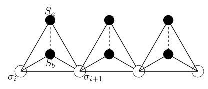
The diamond chain described via the Ising-Heisenberg model comprises a combination of Ising spins located at nodes and interstitial anisotropic Heisenberg spins. The single unit cell of the chain is sketched in Fig. (1a). The Hamiltonian operator is formulated as follows:
| (1) |
where is the number of cells, are the Heisenberg interstitial spins interacting via , and ’s are Ising spins interacting via . The longitudinal external magnetic field () operates on Heisenberg (Ising) spins. The Hamiltonian, Eq. (II), is symmetric under the exchange of the Ising spins, i.e. , and Heisenberg spins, that is . Additionally, the asymmetric tetrahedron Ising-Heisenberg (ATIH) chain, Eq. (II), is invariant under internal spin symmetry, i.e. . To this end, we consider two cases where the Heisenberg spin takes and .
The ATIH chain is an exactly solvable model by making use of the decoration-iteration transformation (DIT) introduced by Fisher [31]. The DIT or star-triangle transformation involves replacing parts of a lattice model with simpler, equivalent structures without altering the physical properties or critical behavior of the system. This is achieved by “decorating” the lattice with additional sites or interactions in a way that allows for an exact transformation of the partition function, which describes the statistical properties of the system [4]. The transformed model is easier to analyze or solve, allowing to gain insights into the original, more complex system. For the ATIH chain, the DIT maps it to an effective Ising chain, as described in Fig. (1b).
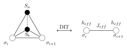
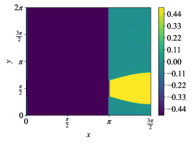
In the following, we restrict our analysis to the case where , which reduces the Heisenberg edge to an type interaction. Fig. (2a) shows the phase diagram of the ATIH spin-() chain under the following new set of parameters
| (2) |
which restrict the system in a region with competing interaction parameters, i.e. , and , leading to several ground state energies. Outside this region there are no new phases [30].
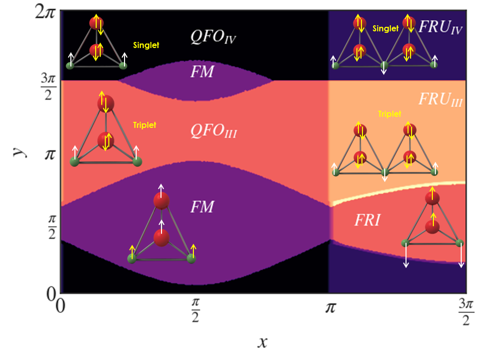
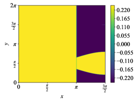
For the ATIH spin-() chain we use the following parameters
| (3) |
to draw the phase diagram represented in Fig. (2b). This re-parametrization essentially maps the original interaction parameters , , , and into a new coordinate system defined by and , facilitating a more tractable exploration of the model’s behavior across different parameter regimes. The mapping reveals critical points where multiple phases converge and provides a clearer understanding of the phase transitions within the ATIH chain [30].
III Figures of Merit
We analyze the phase diagram of the ATIH chain, Eq. (II), using tools from quantum information theory, such as entanglement measures and phase space methods, i.e. the Wigner function. The density matrix of a single cell , comprised by two Ising nodes located at sites () and two Heisenberg nodes (), described by the ATIH model, Eq. (II), can be written as:
| (4) |
with being the dimension of the single cell’s Hilbert space, denoting the identity matrix and at site (and site ). In the same fashion, represent the spin operator with and . For the homogeneous case, i.e. spin, and for the spin inhomogeneous chain . The averages in the spin-spin correlation functions is taken over the ground state of the ATIH chain, Eq. (II), and they can be calculated using the transfer matrix approach outlined in Appendix (B). The detailed expression of the density matrix, Eq. (4), is provided in Appendix (C), from which we can compute various information-theoretic quantities, such as the entanglement measures and the Wigner function.
Lower bound concurrence.
Quantifying the entanglement in quantum systems is a complex task and remains an active area of research in quantum information science [78]. For bipartite qubit systems, analytical formulas for measuring the entanglement are well known, i.e. entanglement of formation, and Wootters concurrence [79]. However, the situation is delicate for higher dimensional quantum systems with multi-parties, for which the single cell of the ATIH chain, Eq. (II), falls into. The entanglement in this case is estimated through lower bounds.
For an -partite quantum state , residing in a composite Hilbert space represented by multiple tensor products of , i.e. , a foundational lower bound for the concurrence has been established [80, 81]. It is expressed as
| (5) |
where the term denotes the number of bipartitions possible within an -partite system. encodes this lower limit for , encapsulating the summation over all bipartite splits indicated by the indices . Here, measures the entanglement across a partition , assuming a uniform dimension across each segment.
The individual concurrences are determined through a widely recognized formula [79]:
| (6) |
where represents the square roots of the top four eigenvalues, sorted in descending order, of the matrix . The modified state is defined as , where , with and are the generators of the special orthogonal group .
The peculiarity of the lower bound , Eq. (5), is its connection with separability. When , the quantum state is fully separable. Thus, for non-zero values of some entanglement is present in the system. The lower bound concurrence, Eq. (5), has been useful in several scenarios, such as studying the statics and dynamics of multipartite entanglement in qubit and ququart systems [19, 18], identification of quantum resource for quantum teleportation [82], as well as studying the performance of quantum heat engines [83].
Phase space techniques.
The Wigner function initially served to depict quantum states in phase space with continuous variables. However, for discrete systems, numerous methods have been devoloped to map these quantum systems onto a phase space framework within a discrete-dimensional Hilbert space. In this context, we adopt the approach proposed by Tilma et al [84], which extends the Wigner function’s applicability to arbitrary quantum states. According to this framework, the Wigner function is formulated using the displacement operator and the parity operators as
| (7) |
where forms the kernel of this function, is the density matrix describing the system and represents a complete parametrization of the phase space such that and are defined in terms of coherent states and . A distribution can describe a Wigner function over a phase space parametrized by a set of ’s, if there exists a kernel that generates according to the Weyl rule
| (8) |
and, as stated in [84], also satisfy the Stratonovich-Weyl correspondences, which articulate several foundational properties of the Wigner function. Primarily, they allow for a bi-directional reconstruction between the density matrix and its representation through a precise mathematical mapping. This mapping not only facilitates the transition from to via the trace formula but also enables the reconstruction of from by integrating over with the kernel . Another critical aspect of these correspondences is the reality and normalization to unity of , ensuring that it always represents a valid quantum state. Additionally, the invariance of under global unitary operations implies a corresponding invariance in , preserving the physical characteristics of the quantum state within the phase space. Lastly, a distinctive feature of the Wigner function is its ability to quantify the overlap between two states and . This is executed through a definite integral over via which highlights a unique property that sets the Wigner function apart in the analysis of quantum states.
An extension of Eq. (8) to finite-dimensional systems requires the construction of a kernel that reflects the symmetries of the system at hand. For spin systems, Tilma et al [84] argued that their Wigner functions can be generated via a spin representation of SU(2) under the following kernels:
| (9) |
with
| (10) |
where is the dimension of the Hilbert space with being the spin number, , and is a diagonal matrix with entries except the last element . In this case, the operator represents the SU(2) rotations under three angles and :
| (11) |
where the ’s are the generators of the dimensional representation of SU(2). For partite quantum systems, the kernel, Eq. (9), extends as
| (12) |
which becomes hard to visualize, as the number of angles scales with the number of subsystems. Therefore, we work within the equal angle slice approximation, by setting and , which has been argued to capture the salient properties of quantum states [84]. Therefore, under the equal angle slice approximation, the total Wigner function of the ATIH chain, Eq. (II), in a single cell described by the state , Eq. (4), is written as:
| (13) | |||
| (14) | |||
The Wigner function, Eq. (8), may take negative values due to its quasi-probability nature. The negativity of the Wigner function, under the equal angle slice approximation, is defined as:
| (15) |
where . This negativity has a profound physical interpretation as it is interpreted as an indicator of non-classical behavior, distinguishing quantum phenomena from their classical counterparts. In the context of quantum entanglement and quantum correlations, the negativity of the Wigner function is a valuable tool for detecting and quantifying some entangled states [85, 86]. In what follows, Equations 8, 5 and 15 will be our main figures of merit.
IV Results and discussions
Homogeneous ATIH chain.
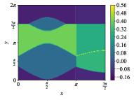
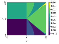
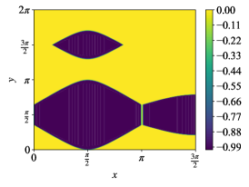
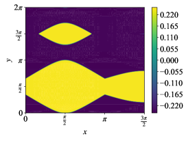
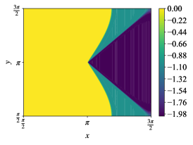
We begin by examining the phase diagram for the spin ATIH chain, Eq. (II). In Fig. (3a), we present the average value of Wigner function, Eq. (13), across the phase space spanned by under the equal angle slice approximation. The Wigner function can effectively capture the entire phase diagram and all the phase boundaries (c.f Fig. (2a)). Furthermore, each phase within the diagram is characterized by distinct values of the Wigner function, which vary from positive to negative based on the parameters . Here, the equal angle slice approximation is a good simplification for capturing the salient critical features of the spin ATIH model, Eq. (II), without the need to explore all the phase space which is computationally exhaustive.
Approaching the phase boundaries, the Wigner function tends to maximize either its negative or positive value, depending on the crossing. For instance, the QFO IV - FM crossing is characterized by high-negativity boundary, while the FRI - FRU III boundary is highly positive. This behavior underscores the importance of exploring the Wigner function on both its negative and positive parts to gain a comprehensive understanding of the phase diagram of the system.
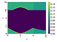
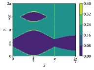
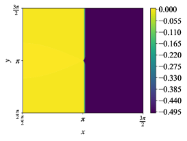
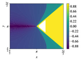
The negativity of the Wigner function, Eq. (15) is depicted in Fig. (3b) under the equal angle slice approximation. The negativity recognize most of the phases with distinctive values, while missing three phase boundaries, i.e. the FRI-, the , and the FM-QFO III phase boundaries, which are captured by the positive part of the Wigner function as shown in panel (3a). Here, the equal angle slice approximation is not adequate to properly quantify the negativity of the Wigner function in the system as we would expect all the phases of matter, except the FM and FRI phases, to have negative Wigner functions. Our expectation comes from the fact that in these phases the Heisenberg nodes responsible for the “quantum” effects in the model are described by entangled states (c.f. Equations 21, 22, 23 and 24), which are known to have a negative Wigner function [87]. We confirm this in panel (3c) where we drop the equal angle slice and compute the negativity of the Wigner function, Eq. (15), over the entire phase space spanned by the angles . We see that the Wigner function is negative over the entire phase diagram except in the coherence-free phases, i.e. the FM and FRI phases. Furthermore, the phase boundaries are more pronounced, including the continuous phase transition line, by a maximum amount of negativity.
Computing the Wigner function over an 8-dimensional phase space is intractable. Therefore, to generate the data in panel (3c) we used statistical approximations via Monte Carlo integration to estimate the values of integrals based on random sampling [88]. The method is particularly useful for dealing with high-dimensional integrals where traditional numerical integration methods become inefficient or infeasible [89]. The method involves generating random points in the domain of the integral and then estimating the integral based on the average value of the function at these points [90].
The effectiveness of Monte Carlo integration increases with the number of dimensions, making it highly suitable for integrals in spaces with dimensions as high as eight or more. This suitability arises because, unlike many deterministic methods, the convergence rate of Monte Carlo integration does not directly depend on the number of dimensions; it depends only on the number of samples, converging with a rate of , where is the number of random samples. This makes it particularly powerful for tackling complex, high-dimensional problems where the geometry or volume of the integration region is complicated [91].
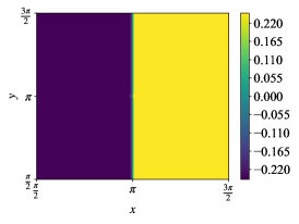
To assess the versatility of the Wigner function approach, we discuss it in light of the lower bound concurrence, Eq. (5), shown in panel (3d). This entanglement measure characterizes the phase diagram (2a) into a entangled and unentangled region. Accordingly, the lower bound concurrence, Eq. (5), splits the phase diagram into three regions: one with zero entanglement, which describes the FM and FRI phases, another with maximum value describing the and phases, and an intermediate region describing and . However, unlike the Wigner function that assign a distinctive value for each phase of matter, the lower bound concurrence, Eq. (5), fails to distinguish between phases of matter in a given entangled (unentangled) region. This shows the utility of the Wigner function approach compared to the lower bound concurrence.
At a closer inspection of panel (3c) and (3d), we see that the negativity of the Wigner function, Eq. (15), follows a pattern similar to the lower bound concurrence, Eq. (5), but on a different scale. However, while the negativity of the Wigner function remains consistent across all entangled phases, the lower bound concurrence provides a finer distinction, differentiating between maximally entangled QFO states and entangled FRU states. This limitation in the negativity of the Wigner function stems from the Monte Carlo approximation, which computes average values of the integrals and could potentially introduce bias. The reported results support the connection between the entanglement and the presence of negativity in the Wigner function, laying a solid foundation for further exploration of how negativity in phase space correlates with entanglement.
Inhomogeneous ATIH chain.
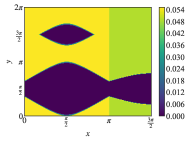
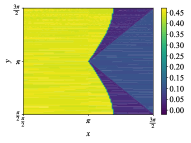
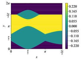
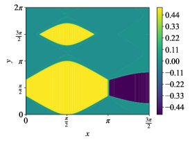
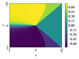
We shift our focus to the inhomogeneous spin chain. Similarly with the homogeneous case, we employ the equal angle slice approximation to explore the phase diagram of the system (c.f. Fig (2b)). Interestingly, this approximation is limited in this case as shown in Fig (4a), where the Wigner function fails to accurately describe the critical properties of the system. The equal angle slice method, like any approximation, sacrifices precision for computational ease. For inhomogeneous quantum systems, this can lead to issues including loss of information in non-uniform areas of the phase space, rendering the results dependent on the chosen slices. Consequently, the approximation does not capture the complete features and detailed structure of the Wigner function.
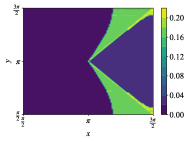
Given these limitations, we abandon the equal angle slice and instead compute the average Wigner function across the entire phase space spanned by the angles as illustrated in Fig. (4b). This approach provides a more accurate representation of the system’s phase diagram. It distinctly highlights the phase boundaries, particularly those delineating regions of positive and negative Wigner function, such as between QFO II - QFO III. However, the phase boundary is less visible due to its positioning between the FRU and QFO phases, which are characterized by a predominantly high positive Wigner function, complicating its detection.
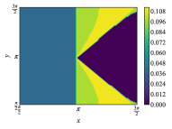
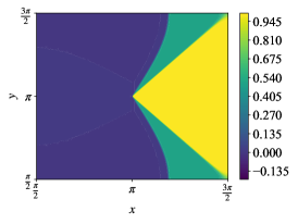
Fig. (4c) and (4d) highlights the negative regions of the Wigner function across the entire phase space using the Monte Carlo approximation for computing integrals and the lower bound concurrence, respectively, for the spin ATIH model. Negative values are localized in phases of matter where the Heisenberg nodes correspond to Bell states, specifically the QFO I and QFO II states (see Equations 53 and 54), which exhibit high entanglement as shown in panel (4d). However, the negativity of the Wigner function fail to distinguish between the FRU and QFO III phases, which involve generalized-Bell states (see Equations 58 and 55) and are also entangled according to panel (4d). This suggests that the lack of negative regions in the Wigner function does not necessarily indicate an absence of entanglement in those areas of phase space. These results call for a profound analysis of Wigner negativity and entanglement in high-dimensional states. The role of Wigner negativity in quantum systems remains a vibrant open question, particularly in exploring its potential to measure entanglement and other quantum informational resources. The measurement and practical utilization of Wigner negativity can have implications for quantum computing and quantum communication protocols.
V Conclusion
We have analyzed the phase diagrams of spin and spin Ising-Heisenberg chains through the lens of the Wigner function. Our results have illuminated the distinct roles played by the negative and positive parts of the Wigner function in revealing the complex phase structures and boundaries of these chains. The comparative analysis with entanglement concurrence has not only validated our findings but also highlighted the strengths and limitations of each approach in revealing the phase diagram of the systems.
The versatility of the equal angle slice approximation in the homogeneous spin chain, as opposed to the necessity of a full phase space integration for the inhomogeneous spin chain, underlines the crucial influence of the quantum system homogeneity on phase space analysis. These insights pave the way for more nuanced approaches to studying quantum systems, particularly in understanding the interplay between system properties and the choice of phase space methods.
Our results lay the foundation for the inspection of a profound relationship between the negativity of the Wigner function and entanglement in quantum many-body systems. This investigation aims to unravel the underlying properties of quantum matter, with a specific focus on how entanglement arise in various quantum phases and its manifestation in phase space. By bridging the gap between Wigner function negativity and quantum entanglement, we aspire to develop a more comprehensive framework for detecting and characterizing the properties of quantum matter. This endeavor will not only enrich our understanding of quantum phase transitions but also contribute significantly to the broader field of quantum physics, potentially influencing the development of quantum computing and information processing technologies.
Acknowledgements
Z.M. acknowledge support from the National Science Center (NCN), Poland, under Project No.. S.D. acknowledges support from the John Templeton Foundation under Grant No. 62422. B.G. acknowledge support from the National Science Center (NCN), Poland, under Project No.. This research is supported through computational resources of HPC-MARWAN provided by CNRST.
Appendix A Spectrum of the ATIH chain
We report here the ground state properties of the ATIH model for the homogeneous and inhomogeneous .
Homogeneous ATIH chain.
To study the phase diagram of the ATIH chain we diagonalize the Hamiltonian, Eq. (II). The introduction of the notations and enables us to recast the Hamiltonian as
| (16) |
where diag() represent the diagonal elements of the Hamiltonian, Eq. (II), with the eigenvalues:
| (17) | ||||
| (18) |
with
| (19) | ||||
| (20) |
The corresponding eigenstates in terms of standard basis are given respectively by:
| (21) | ||||
| (22) | ||||
| (23) | ||||
| (24) |
with
| (25) | ||||
| (26) |
The phase diagram of ATIH spin- displays a rich variety of quantum states and phase transitions due to the complex interplay of the Ising and Heisenberg interactions. Four distinct quantum phases of matter are identified: Quantum Ferromagnetic (QFO), Frustrated Ferromagnetic (FRU), Ferromagnetic (FM), and Ferrimagnetic (FRI). Their corresponding quantum state are given by
| (27) | ||||
| (28) | ||||
| (29) | ||||
| (30) | ||||
| (31) | ||||
| (32) | ||||
| (33) | ||||
| (34) |
where the product is carried over all sites. The first element in the product corresponds to the Ising edge which can take only two possible values , while the second element represents the Heisenberg edge. The Quantum Ferromagnetic phases are categorized into four types (QFO I-IV), each characterized by unique ground state vector products over all lattice sites, and they differ primarily in the orientation probabilities of spins in the Heisenberg edges, which are determined by the functions and , Eq. (26). These functions highlight the quantum nature of the ferromagnetic state by indicating that up and down orientations have distinct probabilities. Meanwhile, the Frustrated Ferromagnetic states (FRU I-IV) demonstrate non-degenerate characteristics with spin frustration present, indicative of the competition between different interactions within the lattice.
The FM and FRI states are defined by the magnetizations of the Ising and Heisenberg edges. In the FM state, spins are aligned in the same direction, leading to a uniform magnetic moment, whereas in the FRI state, there is an alternating pattern of spins which results in a net magnetization that is less than the saturation magnetization. These phases emerge from the interactions that promote parallel and anti-parallel spin alignments, respectively, illustrating the diverse magnetic behaviors that can arise from the interplay of Ising and Heisenberg interactions in low-dimensional quantum systems.
Inhomogeneous ATIH chain.
We consider the Heisenberg edge with in the ATIH model, Eq. (II). Accordingly, the diagonalized Hamiltonian can be written as
| (35) |
with the following eigenvalues
| (36) | ||||
| (37) | ||||
| (38) | ||||
| (39) | ||||
| (40) |
The corresponding eigenstates in the computational basis , , , , , , , , are given by:
| (41) | ||||
| (42) | ||||
| (43) | ||||
| (44) | ||||
| (45) | ||||
| (46) | ||||
| (47) | ||||
| (48) | ||||
| (49) |
where
| (50) |
Accordingly, the phase diagram of the ATIH spin-() chain, Eq. (II), is characterized by a series of distinct phases: Ferromagnetic (FM), Ferrimagnetic (FRI), Quantum Ferromagnetic (QFO), and Frustrated (FRU) states, as well as Quantum Ferrimagnetic (QFI) states. described as follows
| (51) | ||||
| (52) | ||||
| (53) | ||||
| (54) | ||||
| (55) | ||||
| (56) | ||||
| (57) | ||||
| (58) |
where the product is carried over all the sites. The first element in the product corresponds to the Ising edge which can take only two possible values , while the second element represents the Heisenberg edge.
The FM state exhibits uniform spin alignment, resulting in maximal magnetization across the chain. Conversely, the FRI state has alternating spin alignment between the Ising spins and the Heisenberg chains, leading to a reduced net magnetization compared to the FM state. The Quantum Ferromagnetic phases are divided into three types (QFO I-III) and are distinguished by their spin configurations and magnetization behaviors, which are functions of the Heisenberg edge’s interaction parameters. These QFO states showcase the quantum effects inherent in the Heisenberg interaction, where spins are entangled, yielding non-classical magnetic properties.
Quantum Ferrimagnetic states (QFI I and II) emerge when the system displays magnetic order that is intermediate between the FM and FRI states, characterized by non-integral values of the total magnetization per unit cell. This indicates a tough balance between ferromagnetic and antiferromagnetic interactions. The FRU state represents a magnetically disordered phase where the spins are subject to geometric frustration, preventing them from settling into a regular pattern. This state is particularly notable in systems with competing interactions where the geometric arrangement of the spins precludes simultaneous minimization of all interaction energies, leading to a degeneracy of ground states and a lack of long-range magnetic order.
Appendix B The ATIH chain thermodynamics
The thermodynamic properties of the ATIH chain are examined using the decoration-iteration transformation, which is a method initially developed by Fisher [31] allows the complex ATIH chain to be mapped into an effective Ising chain (c.f. Fig. (1)) described by the Hamiltonian
| (59) |
thereby enabling a simplification of the partition function which can be written as function of the Boltzmann weights as
| (60) |
where essentially captures the interactions between the Ising spins and the decorated Heisenberg spins, as well as the external magnetic field’s effects on the system. The parameters and are given by:
| (61) | ||||
| (62) | ||||
| (63) |
The explicit formula for is:
| (64) |
The correlation functions at the Ising and Heisenberg sites follow immediately [4]. The magnetization at the Ising site can be written as
| (65) |
with , while the spin-spin correlation function between the Ising nodes is
| (66) |
Here, denotes the distance between the sites and . , and . At the Heisenberg nodes, the spin correlation function are computed through derivatives of the free energy as
| (67) |
where is the external magnetic field acting on the Heisenberg nodes. The spin-spin correlations function between the nodes follow as
| (68) |
where denotes the coupling strengths between the Heisenberg nodes in the direction. Finally, the Ising-Heisenberg spin correlation function
| (69) |
with
| (70) |
The one-body and two-body correlation functions are given by Equations 65 and 66, while the three-body correlation function is written as . is the correlation length of the standard Ising chain given by [92]
| (71) |
Fig. (5) and (6) shows the correlation functions of the ATIH chain, Eq. (II), for the spin and spin case, with respect to the set of parameters Eq. (2) and Eq. (3), respectively.
Appendix C Density matrix
The full expression of the density matrix is written below
| (72) | ||||
References
- Chang et al. [2018] D. E. Chang, J. S. Douglas, A. González-Tudela, C.-L. Hung, and H. J. Kimble, Colloquium: Quantum matter built from nanoscopic lattices of atoms and photons, Review of Modern Physics 90, 031002 (2018).
- Zeng et al. [2019] B. Zeng, X. Chen, D.-L. Zhou, X.-G. Wen, et al., Quantum information meets quantum matter (Springer, 2019).
- Swan et al. [2022] M. Swan, R. P. Dos Santos, and F. Witte, Quantum matter overview, J 5, 232 (2022).
- Lee [1973] E. W. Lee, Phase transitions and critical phenomena vol 1 exact results, Physics Bulletin 24, 493 (1973).
- Sachdev [2011] S. Sachdev, Quantum Phase Transitions, 2nd ed. (Cambridge University Press, 2011).
- Stern and Lindner [2013] A. Stern and N. H. Lindner, Topological quantum computation—from basic concepts to first experiments, Science 339, 1179 (2013).
- Ayral et al. [2023] T. Ayral, P. Besserve, D. Lacroix, and E. A. Ruiz Guzman, Quantum computing with and for many-body physics, The European Physical Journal A 59, 227 (2023).
- Head-Marsden et al. [2020] K. Head-Marsden, J. Flick, C. J. Ciccarino, and P. Narang, Quantum information and algorithms for correlated quantum matter, Chemical Reviews 121, 3061 (2020).
- Huang et al. [2020] H.-L. Huang, D. Wu, D. Fan, and X. Zhu, Superconducting quantum computing: a review, Science China Information Sciences 63, 1 (2020).
- Wendin [2017] G. Wendin, Quantum information processing with superconducting circuits: a review, Reports on Progress in Physics 80, 106001 (2017).
- Devoret and Schoelkopf [2013] M. H. Devoret and R. J. Schoelkopf, Superconducting circuits for quantum information: An outlook, Science 339, 1169 (2013).
- Atatüre et al. [2018] M. Atatüre, D. Englund, N. Vamivakas, S.-Y. Lee, and J. Wrachtrup, Material platforms for spin-based photonic quantum technologies, Nature Reviews Materials 3, 38 (2018).
- Chirolli and Burkard [2008] L. Chirolli and G. Burkard, Decoherence in solid-state qubits, Advances in Physics 57, 225 (2008).
- Siddiqi [2021] I. Siddiqi, Engineering high-coherence superconducting qubits, Nature Reviews Materials 6, 875 (2021).
- Touil and Deffner [2020] A. Touil and S. Deffner, Quantum scrambling and the growth of mutual information, Quantum Science and Technology 5, 035005 (2020).
- Touil and Deffner [2021] A. Touil and S. Deffner, Information scrambling versus decoherence—two competing sinks for entropy, PRX Quantum 2, 010306 (2021).
- Mzaouali and El Baz [2019] Z. Mzaouali and M. El Baz, Long range quantum coherence, quantum & classical correlations in Heisenberg XX chain, Physica A: Statistical Mechanics and its Applications 518, 119 (2019).
- Abaach et al. [2021] S. Abaach, M. El Baz, and M. Faqir, Pairwise quantum correlations in four-level quantum dot systems, Physics Letters A 391, 127140 (2021).
- Abaach et al. [2022] S. Abaach, M. Faqir, and M. El Baz, Long-range entanglement in quantum dots with fermi-hubbard physics, Physical Review A 106, 022421 (2022).
- Deffner [2021] S. Deffner, Energetic cost of hamiltonian quantum gates, Europhysics Letters 134, 40002 (2021).
- Śmierzchalski et al. [2024] T. Śmierzchalski, Z. Mzaouali, S. Deffner, and B. Gardas, Efficiency optimization in quantum computing: balancing thermodynamics and computational performance, Scientific Reports 14, 4555 (2024).
- MacFarlane et al. [2003] A. G. J. MacFarlane, J. P. Dowling, and G. J. Milburn, Quantum technology: the second quantum revolution, Philosophical Transactions of the Royal Society of London. Series A: Mathematical, Physical and Engineering Sciences 361, 1655 (2003).
- Bandyopadhyay [2005] S. Bandyopadhyay, Computing with spins: from classical to quantum computing, Superlattices and Microstructures 37, 77 (2005).
- Savary and Balents [2016] L. Savary and L. Balents, Quantum spin liquids: a review, Reports on Progress in Physics 80, 016502 (2016).
- Zhou et al. [2017] Y. Zhou, K. Kanoda, and T.-K. Ng, Quantum spin liquid states, Review of Modern Physics 89, 025003 (2017).
- Chauhan et al. [2023] A. Chauhan, A. Maity, C. Liu, J. Sonnenschein, F. Ferrari, and Y. Iqbal, Quantum spin liquids on the diamond lattice, Physical Review B 108, 134424 (2023).
- Okamoto and Ichikawa [2002] K. Okamoto and Y. Ichikawa, Inversion phenomena of the anisotropies of the hamiltonian and the wave-function in the distorted diamond type spin chain, Journal of Physics and Chemistry of Solids 63, 1575 (2002), proceedings of the 8th ISSP International Symposium.
- Jaščur and Strečka [2004] M. Jaščur and J. Strečka, Spin frustration in an exactly solvable Ising–Heisenberg diamond chain, Journal of Magnetism and Magnetic Materials 272-276, 984 (2004), proceedings of the International Conference on Magnetism (ICM 2003).
- Čanová et al. [2006] L. Čanová, J. Strečka, and M. Jaščur, Geometric frustration in the class of exactly solvable Ising–Heisenberg diamond chains, Journal of Physics: Condensed Matter 18, 4967 (2006).
- Valverde et al. [2008] J. Valverde, O. Rojas, and S. de Souza, Phase diagram of the asymmetric tetrahedral Ising–Heisenberg chain, Journal of Physics: Condensed Matter 20, 345208 (2008).
- Fisher [1959] M. E. Fisher, Transformations of Ising Models, Physical Review 113, 969 (1959).
- Honecker and Läuchli [2001] A. Honecker and A. Läuchli, Frustrated trimer chain model and in a magnetic field, Physical Review B 63, 174407 (2001).
- Kikuchi et al. [2003] H. Kikuchi, Y. Fujii, M. Chiba, S. Mitsudo, and T. Idehara, Magnetic properties of the frustrated diamond chain compound cu3 (co3) 2 (oh) 2, Physica B: Condensed Matter 329, 967 (2003).
- Kikuchi et al. [2004] H. Kikuchi, Y. Fujii, M. Chiba, S. Mitsudo, T. Idehara, and T. Kuwai, Experimental evidence of the one-third magnetization plateau in the diamond chain compound cu3 (co3) 2 (oh) 2, Journal of magnetism and magnetic materials 272, 900 (2004).
- Kikuchi et al. [2005a] H. Kikuchi, Y. Fujii, M. Chiba, S. Mitsudo, T. Idehara, T. Tonegawa, K. Okamoto, T. Sakai, T. Kuwai, and H. Ohta, Experimental observation of the 1/3 magnetization plateau in the diamond-chain compound cu 3 (co 3) 2 (oh) 2, Physical Review Letters 94, 227201 (2005a).
- Kikuchi et al. [2005b] H. Kikuchi, Y. Fujii, M. Chiba, S. Mitsudo, T. Idehara, T. Tonegawa, K. Okamoto, T. Sakai, T. Kuwai, K. Kindo, et al., Magnetic properties of the diamond chain compound cu3 (co3) 2 (oh) 2, Progress of Theoretical Physics Supplement 159, 1 (2005b).
- Ohta et al. [2003] H. Ohta, S. Okubo, T. Kamikawa, T. Kunimoto, Y. Inagaki, H. Kikuchi, T. Saito, M. Azuma, and M. Takano, High field esr study of the s= 1/2 diamond-chain substance cu3 (co3) 2 (oh) 2 up to the magnetization plateau region, Journal of the Physical Society of Japan 72, 2464 (2003).
- Okubo et al. [2004a] S. Okubo, T. Kamikawa, T. Kunimoto, Y. Inagaki, H. Ohta, H. Nojiri, and H. Kikuchi, Submillimeter and millimeter wave esr measurements of diamond-chain substance cu3 (co3) 2 (oh) 2, Journal of magnetism and magnetic materials 272, 912 (2004a).
- Ohta et al. [2004] H. Ohta, S. Okubo, Y. Inagaki, Z. Hiroi, and H. Kikuchi, Recent high field esr studies of low-dimensional quantum spin systems in kobe, Physica B: Condensed Matter 346, 38 (2004).
- Okubo et al. [2004b] S. Okubo, H. Ohta, Y. Inagaki, and T. Sakurai, High-field esr systems in kobe, Physica B: Condensed Matter 346, 627 (2004b).
- Guillou et al. [2002] N. Guillou, S. Pastre, C. Livage, and G. Férey, The first 3-d ferrimagnetic nickel fumarate with an open framework:[ni 3 (oh) 2 (o 2 c–c 2 h 2–co 2)(h 2 o) 4]· 2h 2 o, Chemical Communications , 2358 (2002).
- Jeschke et al. [2011] H. Jeschke, I. Opahle, H. Kandpal, R. Valentí, H. Das, T. Saha-Dasgupta, O. Janson, H. Rosner, A. Brühl, B. Wolf, et al., Multistep approach to microscopic models for frustrated quantum magnets: The case of the natural mineral azurite, Physical Review Letters 106, 217201 (2011).
- roj [2011] Exactly solvable mixed-spin Ising-Heisenberg diamond chain with biquadratic interactions and single-ion anisotropy, author=Rojas, Onofre and De Souza, SM and Ohanyan, Vadim and Khurshudyan, Martiros, Physical Review B 83, 094430 (2011).
- Carvalho et al. [2019] I. Carvalho, J. Torrico, S. de Souza, O. Rojas, and O. Derzhko, Correlation functions for a spin-12 Ising-XYZ diamond chain: Further evidence for quasi-phases and pseudo-transitions, Annals of Physics 402, 45 (2019).
- Zheng et al. [2022] Y.-D. Zheng, Z. Mao, and B. Zhou, Optimal dense coding and quantum phase transition in Ising-XXZ diamond chain, Physica A: Statistical Mechanics and its Applications 585, 126444 (2022).
- Pereira et al. [2008] M. Pereira, F. de Moura, and M. Lyra, Magnetization plateau in diamond chains with delocalized interstitial spins, Physical Review B 77, 024402 (2008).
- Pereira et al. [2009] M. Pereira, F. de Moura, and M. Lyra, Magnetocaloric effect in kinetically frustrated diamond chains, Physical Review B 79, 054427 (2009).
- Ananikian et al. [2012] N. Ananikian, H. Lazaryan, and M. Nalbandyan, Magnetic and quantum entanglement properties of the distorted diamond chain model for azurite, The European Physical Journal B 85, 1 (2012).
- Lisnii [2011] B. Lisnii, Distorted diamond Ising-Hubbard chain, Low Temperature Physics 37, 296 (2011).
- Seki and Nishimori [2012] Y. Seki and H. Nishimori, Quantum annealing with antiferromagnetic fluctuations, Physical Review E 85, 051112 (2012).
- Simon et al. [2011] J. Simon, W. S. Bakr, R. Ma, M. E. Tai, P. M. Preiss, and M. Greiner, Quantum simulation of antiferromagnetic spin chains in an optical lattice, Nature 472, 307 (2011).
- Meier et al. [2003] F. Meier, J. Levy, and D. Loss, Quantum computing with antiferromagnetic spin clusters, Physical Review B 68, 134417 (2003).
- Troiani et al. [2005] F. Troiani, A. Ghirri, M. Affronte, S. Carretta, P. Santini, G. Amoretti, S. Piligkos, G. Timco, and R. E. P. Winpenny, Molecular engineering of antiferromagnetic rings for quantum computation, Physical Review Letters 94, 207208 (2005).
- Cai et al. [2023] R. Cai, I. Žutić, and W. Han, Superconductor/ferromagnet heterostructures: A platform for superconducting spintronics and quantum computation, Advanced Quantum Technologies 6, 2200080 (2023).
- Fisher [1925] R. A. Fisher, Mathematical proceedings of the Cambridge Philosophical Society, Vol. 22 (1925) pp. 700–725.
- Nielsen and Chuang [2010] M. A. Nielsen and I. L. Chuang, Quantum Computation and Quantum Information: 10th Anniversary Edition (Cambridge University Press, 2010).
- Rojas et al. [2012] O. Rojas, M. Rojas, N. Ananikian, and S. de Souza, Thermal entanglement in an exactly solvable Ising-XXZ diamond chain structure, Physical Review A 86, 042330 (2012).
- Torrico et al. [2014] J. Torrico, M. Rojas, S. De Souza, O. Rojas, and N. Ananikian, Pairwise thermal entanglement in the Ising-XYZ diamond chain structure in an external magnetic field, Europhysics Letters 108, 50007 (2014).
- Abgaryan et al. [2015] V. Abgaryan, N. Ananikian, L. Ananikyan, and V. Hovhannisyan, Entanglement, magnetic and quadrupole moments properties of the mixed spin Ising–Heisenberg diamond chain, Solid State Communications 203, 5 (2015).
- Rojas et al. [2017a] M. Rojas, S. de Souza, and O. Rojas, Entangled state teleportation through a couple of quantum channels composed of XXZ dimers in an Ising-XXZ diamond chain, Annals of Physics 377, 506 (2017a).
- Qiao and Zhou [2015] J. Qiao and B. Zhou, Thermal entanglement of the Ising–Heisenberg diamond chain with Dzyaloshinskii–Moriya interaction*, Chinese Physics B 24, 110306 (2015).
- Kuzmak [2023] A. R. Kuzmak, Entanglement of the Ising–Heisenberg diamond spin-1/2 cluster in evolution, Journal of Physics A: Mathematical and Theoretical 56, 165302 (2023).
- Freitas et al. [2019] M. Freitas, C. Filgueiras, and M. Rojas, The Effects of an Impurity in an Ising-XXZ Diamond Chain on Thermal Entanglement, on Quantum Coherence, and on Quantum Teleportation, Annalen der Physik 531, 1900261 (2019).
- Chakhmakhchyan et al. [2012] L. Chakhmakhchyan, N. Ananikian, L. Ananikyan, and Č Burdík, Thermal entanglement of the spin-1/2 diamond chain, Journal of Physics: Conference Series 343, 012022 (2012).
- Rojas et al. [2017b] O. Rojas, M. Rojas, S. de Souza, J. Torrico, J. Strečka, and M. Lyra, Thermal entanglement in a spin-1/2 Ising-XYZ distorted diamond chain with the second-neighbor interaction between nodal Ising spins, Physica A: Statistical Mechanics and its Applications 486, 367 (2017b).
- Carvalho et al. [2018] I. Carvalho, J. Torrico, S. de Souza, M. Rojas, and O. Rojas, Quantum entanglement in the neighborhood of pseudo-transition for a spin-1/2 Ising-XYZ diamond chain, Journal of Magnetism and Magnetic Materials 465, 323 (2018).
- Gao et al. [2015] K. Gao, Y.-L. Xu, X.-M. Kong, and Z.-Q. Liu, Thermal quantum correlations and quantum phase transitions in Ising-XXZ diamond chain, Physica A: Statistical Mechanics and its Applications 429, 10 (2015).
- Zheng et al. [2018] Y. Zheng, Z. Mao, and B. Zhou, Thermal quantum correlations of a spin-1/2 Ising–Heisenberg diamond chain with Dzyaloshinskii–Moriya interaction*, Chinese Physics B 27, 090306 (2018).
- Cheng et al. [2017] W. Cheng, X. Wang, Y. Sheng, L. Gong, S. Zhao, and J. Liu, Finite-temperature scaling of trace distance discord near criticality in spin diamond structure, Scientific Reports 7, 42360 (2017).
- Faizi and Eftekhari [2014] E. Faizi and H. Eftekhari, Investigation of Quantum Correlations for A S = 1/2 Ising–Heisenberg Model on a Symmetrical Diamond Chain, Reports on Mathematical Physics 74, 251 (2014).
- Ren et al. [2022] Y. Ren, Z. Zhao, X. Yang, G. Wang, Y. Leng, G. Gao, and X. Liu, Quantum Fisher information at finite temperatures and the critical properties in Ising-Heisenberg diamond chain, Results in Physics 37, 105542 (2022).
- Ferry and Nedjalkov [2018] D. K. Ferry and M. Nedjalkov, The Wigner Function in Science and Technology, 2053-2563 (IOP Publishing, 2018).
- Rundle and Everitt [2021] R. P. Rundle and M. J. Everitt, Overview of the phase space formulation of quantum mechanics with application to quantum technologies, Advanced Quantum Technologies 4, 2100016 (2021).
- Mzaouali et al. [2019] Z. Mzaouali, S. Campbell, and M. El Baz, Discrete and generalized phase space techniques in critical quantum spin chains, Physics Letters A 383, 125932 (2019).
- Millen et al. [2023] N. Millen, R. Rundle, J. Samson, T. Tilma, R. Bishop, and M. Everitt, Generalized phase-space techniques to explore quantum phase transitions in critical quantum spin systems, Annals of Physics 458, 169459 (2023).
- Weinbub and Ferry [2018] J. Weinbub and D. K. Ferry, Recent advances in Wigner function approaches, Applied Physics Reviews 5, 041104 (2018).
- Amico et al. [2008] L. Amico, R. Fazio, A. Osterloh, and V. Vedral, Entanglement in many-body systems, Review of Modern Physics 80, 517 (2008).
- Srivastava et al. [2024] A. K. Srivastava, G. Müller-Rigat, M. Lewenstein, and G. Rajchel-Mieldzioć, Introduction to quantum entanglement in many-body systems (2024), arXiv:2402.09523 [quant-ph] .
- Wootters [1998] W. K. Wootters, Entanglement of formation of an arbitrary state of two qubits, Physical Review Letters 80, 2245 (1998).
- Zhu et al. [2012] X.-N. Zhu, M. Li, and S.-M. Fei, Lower bounds of concurrence for multipartite states, in AIP Conference Proceedings, Vol. 1424 (American Institute of Physics, 2012) pp. 77–86.
- Espoukeh and Pedram [2015] P. Espoukeh and P. Pedram, The lower bound to the concurrence for four-qubit w state under noisy channels, International Journal of Quantum Information 13, 1550004 (2015).
- Abaach et al. [2023] S. Abaach, Z. Mzaouali, and M. El Baz, Long distance entanglement and high-dimensional quantum teleportation in the fermi–hubbard model, Scientific Reports 13, 964 (2023).
- El Hawary and El Baz [2023] K. El Hawary and M. El Baz, Performance of an XXX Heisenberg model-based quantum heat engine and tripartite entanglement, Quantum Information Processing 22, 190 (2023).
- Tilma et al. [2016] T. Tilma, M. J. Everitt, J. H. Samson, W. J. Munro, and K. Nemoto, Wigner functions for arbitrary quantum systems, Physical Review Letters 117, 180401 (2016).
- Kenfack and Życzkowski [2004] A. Kenfack and K. Życzkowski, Negativity of the wigner function as an indicator of non-classicality, Journal of Optics B: Quantum and Semiclassical Optics 6, 396 (2004).
- Siyouri [2016] F. Siyouri, The negativity of wigner function as a measure of quantum correlations, Quantum Information Processing 15, 4237 (2016).
- Davis et al. [2021] J. Davis, M. Kumari, R. B. Mann, and S. Ghose, Wigner negativity in spin- systems, Physical Review Research. 3, 033134 (2021).
- Weinzierl [2000] S. Weinzierl, Introduction to monte carlo methods (2000), arXiv:hep-ph/0006269 [hep-ph] .
- Press and Farrar [1990] W. H. Press and G. R. Farrar, Recursive Stratified Sampling for Multidimensional Monte Carlo Integration, Computer in Physics 4, 190 (1990).
- Newman and Barkema [1999] M. E. Newman and G. T. Barkema, Monte Carlo methods in statistical physics (Clarendon Press, 1999).
- Kroese et al. [2013] D. P. Kroese, T. Taimre, and Z. I. Botev, Handbook of monte carlo methods (John Wiley & Sons, 2013).
- Baxter [2016] R. J. Baxter, Exactly solved models in statistical mechanics (Elsevier, 2016).