From Generalization Analysis to Optimization Designs for State Space Models

Abstract

A State Space Model (SSM) is a foundation model in time series analysis, which has recently been shown as an alternative to transformers in sequence modeling. In this paper, we theoretically study the generalization of SSMs and propose improvements to training algorithms based on the generalization results. Specifically, we give a data-dependent generalization bound for SSMs, showing an interplay between the SSM parameters and the temporal dependencies of the training sequences. Leveraging the generalization bound, we (1) set up a scaling rule for model initialization based on the proposed generalization measure, which significantly improves the robustness of the output value scales on SSMs to different temporal patterns in the sequence data; (2) introduce a new regularization method for training SSMs to enhance the generalization performance. Numerical results are conducted to validate our results.

1 Introduction

Sequence modeling has been a long-standing research topic in many machine learning areas, such as speech recognition (Hinton et al., 2012), time series prediction (Li et al., 2019), and natural language processing (Devlin et al., 2019). Various machine learning models have been successfully applied in sequence modeling to handle different types of sequence data, ranging from the (probabilistic) Hidden Markov model (Baum and Petrie, 1966) to deep learning models, e.g., Recurrent Neural Networks (RNNs), Long Short-Term Memory units (Hochreiter and Schmidhuber, 1997), Gated Recurrent Unit (Chung et al., 2014), and transformers (Vaswani et al., 2017). In this paper, we focus on the state space model (SSM), which has a simple mathematical expression: $h^{\prime}(t)=Ah(t)+Bx(t),y(t)=Ch(t)+Dx(t)$ where $h(t)$ is the hidden state, $x(t)$ is the input sequence, $y(t)$ is the output sequence and $A,B,C,D$ are trainable parameters. To simplify the analysis, we omit the skip connection by letting $D=0$. In fact, our analysis can also applied to the case when $D$ is included (see the discussions in Section 4.2). Recent studies have demonstrated the power of SSMs in deep learning. For example, it was shown in Gu et al. (2022a) that by a new parameterization and a carefully chosen initialization, the structured state space sequence (S4) model achieved strong empirical results on image and language tasks. Following the S4 model, more variants of SSMs are proposed, e.g., diagonal SSMs (Gu et al., 2022b, Gupta et al., 2022) S5 (Smith et al., 2023), H3 (Fu et al., 2023), GSS (Mehta et al., 2023), Hyena Hierarchy (Poli et al., 2023), and Mamba (Gu and Dao, 2023).

Theoretical analysis and understanding of the approximation and optimization of SSMs are well studied in the literature such as (Li et al., 2021; 2022, Gu et al., 2022a; 2023). Since the SSM can be regarded as a continuous linear RNN model (Li et al., 2022), most generalization analysis of SSMs is based on the generalization theory of RNNs (Zhang et al., 2018, Chen et al., 2019, Tu et al., 2019). However, these previous works did not study the effects of the temporal dependencies in the sequence data on the SSM generalization (see more details on the comparison in Section 4.1). As an attempt to understand the relationship between the temporal dependencies and the generalization performance, this paper aims to provide a generalization bound that connects the memory structure of the model with the temporal structure of the data. We can, in turn, use the proposed bound to guide us in designing new algorithms to improve optimization and generalization. Specifically, we discover two roles for the proposed generalization measure: (1) generalization bound as an initialization scheme; (2) generalization bound as a regularization method. The common initialization method for the S4 model and its variants follows from the HiPPO framework (Gu et al., 2022a; 2023), which is based on the prerequisite that the training sequence data is stable. To improve the robustness of the output value scales on SSMs to different temporal patterns in the sequence data, we consider to rescale the initialization of SSMs with respect to the generalization measure. This new initialization scheme makes the SSMs more resilient on their initial output value scales to variations in the temporal patterns of the training data. Except for the initialization setup, our generalization bound can also be served as a regularizer. Regularization methods like weight decay and dropout are widely applied to training SSMs, but the hidden state matrix $A$ is not regularized because its imaginary part controls the oscillating frequencies of the basis function $e^{At}B$ (Gu et al., 2022b). By taking into account the interaction between the SSM structure and the temporal dependencies, we introduce a new regularization method based on our bound, and it can be applied to the hidden state space to improve the generalization performance. Combining the initialization scheme and the regularization method, our method is applicable to various tasks, ranging from image classification to language processing, while only introducing a minimal computational overhead. To summarize, our contributions are as follows:

• We provide a data-dependent generalization bound for SSMs by taking into account the temporal structure. Specifically, the generalization bound correlates with the memory structure of the model and the (auto)covariance process of the data. It indicates that instead of the weight or the data norm, it is the interplay between the memory structure and the temporal structure of the sequence data that influences the generalization.

• Based on the proposed generalization bound, we setup an initialization scaling rule by adjusting the magnitude of the model parameters with respect to the generalization measure at initialization. This scaling rule improves the robustness of the initial output value scales on SSMs across different temporal patterns of the sequence data.

• Apart from the initialization scheme, we design a new regularizer for SSMs. Unlike weight decay, our regularizer does not penalize the parameter norm but encourages the model to find a minimizer with lower generalization bound to improve the generalization performance.

2 Related Works

Since a SSM is also a continuous linear RNN, there are three lines of related work: generalization of RNNs, temporal structure analysis on RNNs, and optimization of SSMs.

Generalization of RNNs. Existing works on the generalization of RNNs focus on the generalization error bound analysis. Specifically, in the early two works of Dasgupta and Sontag (1995) and Koiran and Sontag (1998), VC dimension-based generalization bounds were provided to show the learnability of RNNs. In recent studies, Zhang et al. (2018), Chen et al. (2019), Tu et al. (2019) proved norm-based generalization bounds, improving the VC dimension-based bounds by the Rademacher complexity technique (Bartlett and Mendelson, 2002) under the uniform-convergence framework. In the overparameterization settings, it was shown in Allen-Zhu and Li (2019) that RNNs can learn some concept class in polynomial time given that the model size is large enough. These generalization bounds, however, do not take into account the temporal dependencies and their effects on generalization. In this work, we provide a new generalization bound by combining the memory structure of the model and the temporal structure of the data.

Temporal structure analysis on RNNs. Sequence data has long-range temporal dependencies across the time domain, which notably set it apart from non-sequence data. Recent studies have studied the effects of such temporal dependencies on the approximation and optimization of RNNs. For example, in the two works of Li et al. (2021; 2022), a “curse of memory” phenomenon was discovered when using linear RNNs to model the temporal input-output relationships. Particularly, when the target relationship between the input and output has a long-term memory, then both approximation and optimization become extremely challenging. In Wang et al. (2023), the “curse of memory” phenomenon on approximation and optimization was extended to non-linear RNNs based on the temporal relationships. In this paper, we conduct a fine-grained analysis on the effects of the temporal structure analysis on the generalization of RNNs.

Optimization of SSMs. RNN optimization is known for two issues: training stability and computational cost (Bengio et al., 1994, Pascanu et al., 2013). To address these issues and capture the long dependencies efficiently in sequence modeling, the S4 model was proposed by new paraemterization, initialization and discretization (Gu et al., 2022a). Recent variants for the S4 model simplified the hidden state matrix by a diagonal matrix to enhance computational efficiency (Gu et al., 2022b, Gupta et al., 2022, Smith et al., 2023, Orvieto et al., 2023). Regularization methods are also applied for SSMs to prevent overfitting, such as dropout, weight decay and the data continuity regularizer (Qu et al., 2023). However, the principled way to regularize and initialize the parameters still remains to be explored. In this study, we design a new regularization and initialization scheme to improve both optimization and generalization.

3 Preliminaries

In this section, we briefly introduce the SSM in Section 3.1 and the motivation for optimization designs based on the generalization analysis in Section 3.2.

3.1 Introduction to SSMs

In this paper, we consider the following single-input single-output SSM,

$$h^{\prime}(t)=Ah(t)+Bx(t),\quad y(t)=Ch(t),\quad t\geq 0$$ (1)

where $x$ is the input from an input space $\mathcal{X}:=C_{0}(\mathbb{R}_{\geq 0},\mathbb{R})$; $y(t)\in\mathbb{R}$ is the output at time $t$; $h(t)\in\mathbb{R}^{m}$ is the hidden state with $h(0)=0$; $A\in\mathbb{R}^{m\times m},B\in\mathbb{R}^{m\times 1},C\in\mathbb{R}^{1\times m}$ are trainable parameters. Then (1) has an explicit solution $y(t)=\int_{0}^{t}\rho_{\theta}(s)x(t-s)ds$, where $\rho_{\theta}(s):=Ce^{As}B$ with $\theta=(C,A,B)$. The function $\rho_{\theta}(s)$ captures the memory structure of the model and the temporal input-output relationship (Li et al., 2022). For the S4 model and its variants (Gu et al., 2022a; b, Gupta et al., 2022, Gu et al., 2023), (1) is usually discretized by the Zero-Order Hold method, i.e., given a timescale $\Delta\in\mathbb{R}$, $h_{k+1}=\bar{A}h_{k}+\bar{B}x_{k},\quad y_{k}=\bar{C}h_{k},\quad k=0,1,\ldots,$ where $\bar{A}=e^{\Delta\cdot A},\bar{B}=(\bar{A}-\mathbb{I}_{m})A^{-1}B,\bar{C}=C$. Then, $y_{k}=\bar{C}\bar{A}^{k}\bar{B}x_{0}+\bar{C}\bar{A}^{k-1}\bar{B}x_{1}+\ldots+\bar{C}\bar{B}x_{k}=[\bar{K}*x]_{k}$ where $\bar{K}=(\bar{C}\bar{B},\bar{C}\bar{A}\bar{B},\ldots,\bar{C}\bar{A}^{k}\bar{B})$ and $*$ represents to convolution.

3.2 Motivation: a linear regression model

In this subsection, we use a linear regression model on non-sequential data as an example to illustrate the connection between the generalization analysis and the optimization designs. This example then motivates us to extend the connection to SSMs on sequential data.

Linear regression. We consider a simple linear model $y=\theta^{\top}x$ with input $x\in\mathbb{R}^{d}$, output $y\in\mathbb{R}$ and parameter $\theta\in\mathbb{R}^{d}$. Let the training data $\{(x_{i},y_{i})\}_{i=1}^{n}$ be i.i.d. sampled from a distribution $\mathcal{D}$ such that $\|x_{i}\|_{2}=r,|y_{i}|\leq 1(\forall i\in[1:n])$. Define the empirical risk $\mathcal{L}_{n}(\theta):=\frac{1}{n}\sum_{i=1}^{n}(\theta^{\top}x_{i}-y_{i})^{2}$ and the population risk $\mathcal{L}_{\mathcal{D}}(\theta):=\mathbb{E}_{x,y}[(\theta^{\top}x-y)^{2}]$. Then given a norm-constrained space $\Theta:=\{\theta\in\mathbb{R}^{d}:\|\theta\|_{2}\leq R\}$, with probability at least $1-\delta$ over $\mathcal{D}$,

$$\sup_{\theta\in\Theta}|\mathcal{L}_{n}(\theta)-\mathcal{L}_{\mathcal{D}}(\theta)|\leq(rR+1)^{2}\cdot\mathcal{O}(\sqrt{\log(1/\delta)/n}).$$ (2)

This is a well-known norm-based generalization bound based on the Rademacher theory (Mohri et al., 2012), and we provide a proof in Appendix B for completeness. Notice that the key term $r^{2}R^{2}$ in the generalization bound (2) is also an upper bound for the magnitude of the linear model output, i.e., $\sup_{\theta\in\Theta}(\theta^{\top}x_{i})^{2}\leq r^{2}R^{2}$. Thus, we connect the model stability with the generalization bound stability, and this connection induces an initialization scheme for the initialization $\theta^{(0)}$ by setting $\|\theta^{(0)}\|_{2}\sim\mathcal{O}(1/r)$. In particular, if we normalize each input $x_{i}$ such that $r$ is also $\mathcal{O}(1)$, then $\|\theta^{(0)}\|_{2}\sim\mathcal{O}(1)$. Since $\theta^{(0)}\in\mathbb{R}^{d}$, one possible initialization scheme is that $\theta^{(0)}$ follows a Uniform distribution $U[-1/\sqrt{d},1/\sqrt{d}]$, which corresponds to the Kaiming initialization (up to some constant) (He et al., 2015). When treating the term $r^{2}R^{2}$ as a regularizer to improve the generalization, we get the weight decay method, i.e., the $\ell_{2}$ regularization w.r.t. $\|\theta\|_{2}^{2}$. We summarize the above logic chain that connects the generalization analysis with optimization designs in Figure 1.

Figure 1: The logic diagram goes from generalization analysis to optimization designs.

Now for SSMs, we extend the generalization analysis from non-sequential data to sequential data by taking into account the temporal structure of the data. This linear regression example motivates us to apply the same logic diagram (Figure 1) to the SSMs, and this is exactly what we are going to present in the following part of this paper.

4 Main results

In this section, we first give a generalization bound for SSMs in Section 4.1, then we design a new initialization scheme in Section 4.2 based on this proposed bound. Apart from the initialization scheme, we introduce a new regularization method in Section 4.3. Finally, we conduct experiments to test the initialization scheme and the regularization method in Section 4.4.

4.1 A generalization bound of SSMs

In this section, we present a generalization bound for the SSM (1) and reveal the effects of the temporal dependencies on the generalization performance. We show that our bound gives a tighter estimate compared with previous norm-based bounds through a toy example. Following the same notation in Section 3.1, we define the empirical risk ${R}_{n}(\theta)$ and the population risk $R_{x}(\theta)$ as

$${R}_{n}(\theta):=\frac{1}{n}\sum_{i=1}^{n}\left|\int_{0}^{T}{\rho}_{\theta}(T-s)x_{i}(s)ds-y_{i}\right|^{2},\quad R_{x}(\theta):=\mathbb{E}_{x}\left|\int_{0}^{T}{\rho}_{\theta}(T-s)x(s)ds-y\right|^{2}$$

where $T>0$ is some finite terminal time, the training sequence data $\{x_{i}(t)\}_{i=1}^{n}$ are independently sampled from a stochastic process with mean $\mathbb{E}[x(t)]:=\mu(t)$ and covariance $\mathbb{E}[(x(s)-\mu(s))(x(t)-\mu(t))]:=K(s,t)$, and the label $y$ is generated by some underlying functional $H_{T}:\mathcal{X}\xrightarrow{}\mathbb{R}$, i.e., $y=H_{T}(x)$. We assume that $|y|\leq 1$ for any $x\in\mathcal{X}$, otherwise, we truncate the value of the label to $1$. In the next, we make an assumption on the normalized process $\tilde{x}(t):=(x(t)-\mu(t))/\sqrt{K(t,t)}$:

Assumption 1.

The normalized process $\tilde{x}(t)$ is (1): almost surely Hölder continuous, i.e., $\exists L,H>0,s.t.\forall s,t\in[0,T],|\tilde{x}(s)-\tilde{x}(t)|\leq L|s-t|^{H}a.s.$; (2): is $\sigma^{2}$-sub-Gaussian for every $t\in[0,T]$, i.e., $\exists\sigma>0,s.t.\forall u>0,P\left(|\tilde{x}(t)|\geq u\right)\leq 2\exp(-u^{2}/2\sigma^{2})$ for any $t\in[0,T]$.

We leave the discussion of the assumption after the statement of the main theorem. Now we proceed to bound generalization gap $|R_{x}(\theta)-{R}_{n}(\theta)|$ by establishing uniform convergence of the empirical risk to its corresponding population risk, as stated in following theorem:

Theorem 1.

For a SSM $\int_{0}^{T}{\rho}_{\theta}(T-s)x(s)ds$, following notations and settings in Section 3.1 & 4.1, we define $\psi(\Theta):=\sup_{\theta\in\Theta}\int_{0}^{T}\left|{\rho}_{\theta}(T-s)\right|\sqrt{K(s,s)}ds+\sup_{\theta\in\Theta}\left|\int_{0}^{T}{\rho}_{\theta}(T-s)\mu(s)ds\right|$. Then under Assumption 1, given a parameter space $\Theta$ for $\theta$, for any $\delta\in(0,1)$, with probability at least $1-\delta$ over the training sequences,

$$\sup_{\theta\in\Theta}\left|R_{x}(\theta)-{R}_{n}(\theta)\right|\leq(\psi(\Theta)+1)^{2}\cdot\mathcal{O}(\log^{3/2}(Tn/\delta)/{\sqrt{n}}).$$ (3)

Where $\mathcal{O}$ hides a constant that depends on $\sigma,L,H$. The proof is given in Appendix E. We see that this bound decreases to zero as the sample size $n\xrightarrow{}\infty$, provided that the terminal time $T$ is finite and $\psi_{\Theta}$ grows slower than $\sqrt{n}$. For example, when the data statistics (e.g., $\mu(s)$ and $K(s,s)$) are uniformly bounded along the time horizon, by the exponentially decay property of the SSM function $\rho_{\theta}(s)$, we have $\psi_{\Theta}$ is finite, then the generalization bound is $\tilde{\mathcal{O}}(1/\sqrt{n})$, yielding that the mean and variance at each length position together play important roles in generalization analysis.

Proof sketch. The proof is based on Rademacher theory (Bartlett and Mendelson, 2002). The main difficulty is to bound the Rademacher complexity of the SSM function $\int_{0}^{T}{\rho}_{\theta}(T-s)x(s)ds$ for a stochastic process $x(s)$. We first use the Hölder inequality to get an upper bound for the Rademacher complexity w.r.t. the normalized process $\tilde{x}(s)$, then combining Hölder continuity and the heavy-tail property in Assumption 1, we show the finiteness of $\sup_{s\in[0,T]}\tilde{x}(s)$. Finally we use an $\varepsilon$-net argument to give an explicit bound for the Rademacher complexity, which then finishes the proof.

Discussions of Assumption 1. This assumption contains two parts. Hölder continuity is used to bound $\sup_{s\in[0,T]}\tilde{x}(s)$ and the Rademacher complexity of the SSM function class. By the Kolmogorov continuity theorem (Stroock and Varadhan, 1997), Hölder continuity covers a wide range of random process that satisfies certain inequalities for its moments. For the sub-Gaussian property, it ensures $\tilde{x}(s)$ is bounded in a finite time set with high probability. Sub-Gaussian random variables include Gaussian and any bounded variables. Specifically, for image classification tasks with flattened image pixels, if the range of the pixel values is a finite class (e.g., integer numbers from 0 to 255), then the Hölder continuity condition can be dropped. We leave more detailed discussions and provide some concrete examples that satisfy Assumption 1 in Appendix C.

Comparison to previous bounds. Since a SSM is also a continuous linear RNN model, we compare (3) with previous bounds for linear RNNs. A generalization bound $\widetilde{\mathcal{O}}\left(\|x\|_{2}\|B\|_{2}\|C\|_{2}\|A\|_{2}/{\sqrt{n}}\right)$ is provided In Chen et al. (2019), where $\|x\|_{2}$ is the 2-norm of the discrete input sequence. In the continuous case, $\|x\|_{2}$ corresponds to the $L^{2}$ norm w.r.t. a Dirac measure. By changing the matrix 2-norm to matrix 1-norm, Tu et al. (2019) shows another similar generalization bound. These bounds separate the data complexity and the model complexity by the data norm and the model parameter norm individually, and do not account for the temporal dependencies across the time domain. In this work, instead, we incorporate the temporal dependencies via the sequence statistics (mean and variance) to get a generalization bound. Next, we use a toy example to illustrate that our bound gives a tighter estimation. Given a stochastic process $\{x(t)\}_{t\in[0,T]}$ with mean $\mu(t)$ and covariance $K(s,t)$, we consider the following two upscale transformations (by increasing $T$ to $2T$):

1. left zero padding: $x_{1}(t)=0,\ t\in[0,T);\quad x_{1}(t)=x(t-T),\ t\in[T,2T]$

2. right zero padding: $x_{2}(t)=x(t),\ t\in[0,T];\quad x_{2}(t)=0,\ t\in(T,2T]$

Then the two SSM outputs are given by $y_{i}(2T)=\int_{0}^{2T}{\rho}_{\theta}(2T-s)x_{i}(s)ds$ for $i=1,2$. Hence,

$$y_{1}(2T)=C\int_{0}^{T}e^{A(T-s)}Bx(s)ds,\quad y_{2}(2T)=Ce^{AT}\int_{0}^{T}e^{A(T-s)}Bx(s)ds.$$

We see that the magnitude of $y_{1}(2T)$ and $y_{2}(2T)$ differs with an exponential factor $e^{AT}$. Since all the eigenvalues of $A$ have negative real part, $y_{2}(2T)\xrightarrow{}0$ as $T$ increases. Hence, the right zero padding transformation degenerates the SSM function class to a zero function class for large $T$, inducing a minimal generalization gap that only contains the statistical sampling error (see (3) by letting $K(s,s)=\mu(s)=0$). Therefore, a desired generalization bound should reflect such a difference caused by the different temporal dependencies. However, previous norm-based generalization bounds do not capture such a difference for these two transformations as they produce the same $L^{2}$ norm for the input sequence. Let us see what happens for our proposed generalization measure. For the left zero padding, the key term in (3) becomes

$$\int_{0}^{T}\left|Ce^{A(T-s)}B\right|\sqrt{K(s,s)}ds+\left|\int_{0}^{T}Ce^{A(T-s)}B\mu(s)ds\right|+1$$ (4)

For the right zero padding, the key term in (3) becomes

$$\int_{0}^{T}\left|Ce^{AT}e^{A(T-s)}B\right|\sqrt{K(s,s)}ds+\left|\int_{0}^{T}Ce^{AT}e^{A(T-s)}B\mu(s)ds\right|+1$$ (5)

The detailed derivations are given in Appendix D. By the same argument, our bound (3) indeed captures the difference on the magnitude of the generalization performance for these two sequence transformations. In particular, as $T\xrightarrow{}\infty$, (5) reduces to $1$, which yields a minimal generalization gap as expected for the zero function class. In that sense, we get a tighter bound for the SSMs.

Zero shot transferability. A benefit of SSMs is the zero-shot transferability to other sampling frequencies (i.e., the timescale measure in continuous case). For example, for a SSM function $y_{T}=\int_{0}^{T}{\rho}_{\theta}(T-s)x(s)ds$, if we downscale the input sequence $x(s)$ by half of the sampling frequency, then the SSM output becomes $y_{T}=\int_{0}^{T/2}{\rho}_{\theta}(T-2s)x(2s)ds$, which equals to $\int_{0}^{T}\frac{1}{2}{\rho}_{\theta}(T-s)x(s)ds$. Now for a new SSM parameter $\tilde{\theta}=(2C,A,B)$, we have $\rho_{\tilde{\theta}}(s)=2\rho_{\theta}(s)$, indicating that by simply modifying the SSM parameters, one can transfer the model to half the sampling frequency while keeping the output invariant. One advantage for our generalization measure is that it is also zero shot transferable. To see this, we use the same example here. Under the downscale sampling, both $\int_{0}^{T}\left|{\rho}_{\theta}(T-s)\right|\sqrt{K(s,s)}ds$ and $\left|\int_{0}^{T}{\rho}_{\theta}(T-s)\mu(s)ds\right|$ remain invariant for the new parameter $\tilde{\theta}$ because $\sqrt{K(s,s)}$ and $\mu(s)$ have the same scaling as $x(s)$. Similarly, other sampling frequencies are also zero shot transferable for our generalization measure by simply adjusting the SSM parameters.

4.2 Generalization bound as an initialization scheme

In this section, we design a scaling rule for the SSM parameters at initialization based on the generalization bound (3). This new initialization scheme improves the robustness of the initial output value scales on SSMs across different temporal patterns of the sequence data.

Our proposed initialization scheme is built on the HiPPO based initialization (Gu et al., 2023), which is a data independent initialization method. Specifically, the HiPPO framework initializes the hidden state matrices $A,B$ to produce orthogonal basis functions, and the matrix $C$ to be standard normal for training stability. However, the argument for the training stability relies on the prerequisite that the input sequence is constant along the time index (Gu et al. (2023, Corollary 3.4)), which has some limitations in applicability as the long-range dependencies may lead to very different temporal patterns on the input sequence. As the dashed lines in the left and the right part of Figure 2 show, the SSM output value scale and the loss value scale under the HiPPO based initialization vary much across different temporal dependencies, making the loss values inconsistent during training. To address this issue, we follow the logic diagram in Figure 1 by adjusting the generalization complexity to be $\mathcal{O}(1)$. Specifically, we extract the dominant term in the generalization bound (3):

$$\tau(\theta):=\left(\int_{0}^{T}\left|{\rho}_{\theta}(T-s)\right|\sqrt{K(s,s)}ds+\left|\int_{0}^{T}{\rho}_{\theta}(T-s)\mu(s)ds\right|\right)^{2}.$$ (6)

Notice that ${\rho}_{\theta}(s)=Ce^{As}B$, if we rescale $C$ to $\xi C$ for some $\xi\in\mathbb{R}$, we have $\tau(\tilde{\theta})=\xi^{2}\cdot\tau(\theta)$ for $\tilde{\theta}=(\xi C,A,B)$. This induces a new initialization scheme, i.e., once the parameters $\theta=(C,A,B)$ are initialized by the HiPPO method, we rescale $C$ to $\tilde{C}$ such that

$$\tilde{C}=\frac{1}{\sqrt{\tau(\theta)}}\cdot C.$$ (7)

This rescaling method guarantees the SSM output value is bounded at initialization for any stochastic process that satisfies Assumption 1, ensuring the robustness of the initial loss value scales on SSMs across different temporal structures. We formalize the statement in Proposition 1.

Proposition 1.

Consider a SSM $\int_{0}^{T}{\rho}_{\theta}(T-s)x(s)ds$ with $\theta=(C,A,B)$, for any random process $x(s)$ satisfies Assumption 1, let $\tilde{C}$ be given by the rescaling method (7), then for $\tilde{\theta}:=(\tilde{C},A,B)$, we have $\mathbb{E}_{x}\left[\left|\int_{0}^{T}{\rho}_{\tilde{\theta}}(T-s)x(s)ds\right|\right]\leq\mathcal{O}(\sqrt{\log T})$. Here $\mathcal{O}$ hides a constant that only depends on $\sigma$ and $L$ as described in Assumption 1.

The proof is provided in Appendix F. Proposition 1 shows that the expected SSM output value are bounded for any stochastic processes that satisfies Assumption 1, even when the input sequence is not almost surely bounded. This improves the robustness of the output value scales on SSMs in the sense that the scale of the output value does not depend on the variations of the temporal structures. It is worth noting that different from normalization methods such as min-max normalization and standardization, our method only changes the model parameters. This is important because normalization on data numerical values in language tasks can lead to loss of crucial information. For example, mathematical expressions like “$\max(1,9)=9$” have a contextual meaning where normalization may result in the loss of structured information that is essential to understand.

Algorithm 1 Training an $\ell$-layer SSM with the scheme (7)

1:training sequences with length $L$, model dimension $d$, projection matrix $C_{i}$ of $i$-th layer, number of epochs $S$

2:for $s=0$ to $S-1$ do

3:     if $s=0$ then

4:         Sample a minibatch sequence from the training sequences

5:         for $i=1$ to $\ell$ do

6:              Compute mean $\mu_{i}\in\mathbb{R}^{L\times d}$, variance $K_{i}\in\mathbb{R}^{L\times d}$ of the $i$-th layer’s inputs along the batch dimension $\triangleright$ Inputs of the $i$-th layer depend on model parameters of the first $i-1$ layers

7:              Calculate the SSM kernel $k_{i}\in\mathbb{R}^{L\times d}$ by the model parameters of the $i$-th layer

8:              $\tau_{i}\leftarrow\left[|k_{i}|*\sqrt{K_{i}}+|k_{i}*\mu_{i}|\right]_{L}\in\mathbb{R}^{d}$

9:              Averaging over the feature dimension: $\tau_{i}\leftarrow\|\tau_{i}\|_{2}^{2}/d$

10:              Update: $C_{i}\leftarrow{C_{i}}/\sqrt{\tau_{i}}$

11:         end for

12:     end if

13:     Regular training procedure for the updated initialization

14:end for

Implementation for high-dimensional, multi-layer SSMs. In the practical training, the SSMs used for tasks such as image classification or language processing are usually deep and high dimensional ($d>1$), while our initialization scheme (7) is designed based on the one-dimensional shallow SSM. To extend to high-dimensional SSMs, we empirically treat all features to be independent and calculate $\tau(\theta)$ by its average along the feature dimension. For an $\ell$-layer SSM with the initial projection matrix $C_{1},\ldots,C_{\ell}$ at each layer, we first calculate the complexity measure $\tau_{1}$ for the first layer and rescale $C_{1}$ by $C_{1}/\sqrt{\tau_{1}}$. Then we calculate the complexity measure $\tau_{2}$ for the second layer by the updated input sequence of layer 2 and rescale $C_{2}$ by $C_{2}/\sqrt{\tau_{2}}$. We repeat this process until the last layer. We describe the complete procedures in Algorithm 1, where the $|\cdot|$ and $\sqrt{\cdot}$ in Line $7$ represent to element-wise absolute value and element-wise square root respectively. $[\cdot]_{L}$ extracts the last position of an element obtained from the convolution. The extension of our theory to the multi-layer case is an interesting direction, which we leave for future work.

Skip connections and nonlinearities. There are several gaps between the theory and the methodologies in this paper. The first one that the skip connection matrix $D$ is omitted in our defined model (1). This will not affect our generalization bound because we may express the explicit solution for (1) as $y(t)=\int_{0}^{t}(\rho_{\theta}(s)+D\delta(s))x(t-s)ds$ where $\delta(\cdot)$ is a delta function. In that case, the SSM is still a convolution model but with a new kernel function $\rho_{\theta}(s)+D\delta(s)$. However, the initialization scheme (7) only adjusts $C$ and requires the kernel function to be linear in $C$. Hence, (7) may not work well when $Dx(t)$ is much larger than $\int_{0}^{t}\rho_{\theta}(s)x(t-s)ds$. However, we can still derive a proper rescaling scheme for this case. One straightforward way is that we first calculate $\tau(\theta)$ for a given initialization, and then rescale $C,D$ as $C\sqrt{\tau(\theta)}$ and $D/\sqrt{\tau(\theta)}$ respectively. This reinitialization method guarantees that $\tau(\theta)=1$ after rescaling. The second gap is that our theory is for single-layer linear SSMs. When nonlinearities are added, our generalization bound still works for single-layer SSMs if the nonlinearity does not affect the Hölder condition and the sub-Gaussian property (Assumption 1). For Lipschitz (also Hölder continuous) nonlinearities, there are some known examples (see Appendix G) where the sub-Gaussian condition still remains after the nonlinearity.

4.3 Generalization bound as a regularization method

Algorithm 2 Training an $\ell$-layer SSM with the scheme (8)

1:training sequences with length $L$, model dimension $d$, initialization $\theta_{0}$, loss function $\mathcal{L}$, regularization factor $\lambda$, optimizer OPT, number of epochs $S$

2:for $s=0$ to $S-1$ do

3:     Sample a minibatch from the training sequences

4:     Set total complexity $\tau=0$

5:     for $i=1$ to $\ell$ do

6:         Compute mean $\mu_{i}\in\mathbb{R}^{L\times d}$ and variance $K_{i}\in\mathbb{R}^{L\times d}$ for inputs of the $i$-th layer along the batch dimension

7:         Calculate the SSM kernel $k_{i}\in\mathbb{R}^{L\times d}$ by the model parameters of the $i$-th layer

8:         $\tau_{i}\leftarrow\left[|k_{i}|*\sqrt{K_{i}}+|k_{i}*\mu_{i}|\right]_{L}\in\mathbb{R}^{d}$

9:         Averaging over the feature dimension: $\tau_{i}\leftarrow\|\tau_{i}\|_{2}^{2}/d$

10:         Add the complexity of the $i$-th layer: $\tau\leftarrow\tau+\tau_{i}$

11:     end for

12:     Compute the training loss: $\mathcal{L}\leftarrow\mathcal{L}+\lambda\cdot\tau$

13:     Parameters update: $\theta_{i+1}\leftarrow\textsf{OPT}(\theta_{i},\mathcal{L})$

14:end for

15:Updated model parameter $\theta_{s}$

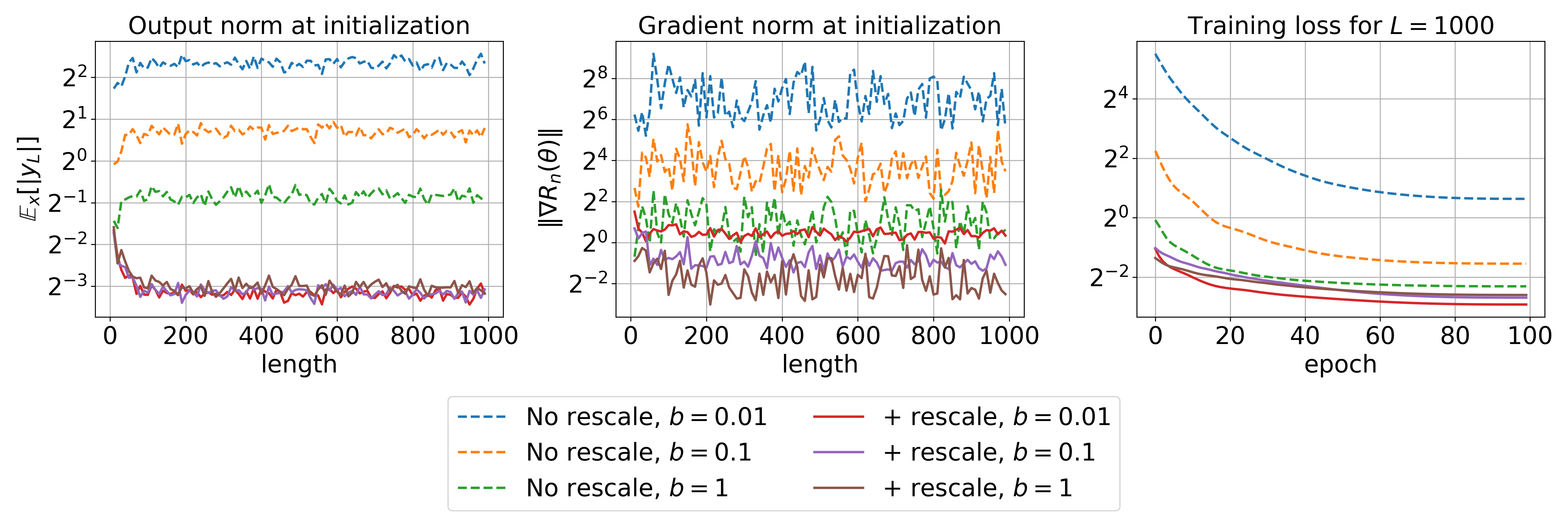
Figure 2: Effects of the initialization scheme (7) on the model output scale, the gradient norm and the training loss under different temporal dependencies by varying the moment coefficient $b=0.01,0.1,1$. (Left) The output $\mathbb{E}_{x}[|y_{L}|]$ at initialization w.r.t. the Gaussian white noise sequence $(x_{1},\ldots,x_{L})$ for length $L$ from $1$ to $1000$; (Middle) The gradient norm $\|\nabla R_{n}(\theta)\|$ at initialization w.r.t. the mean squared error (MSE) for varied sequence length; (Right) The training MSE curve for the Gaussian white noise with length $L=1000$.

In addition to its role as an initialization scheme, the generalization measure can also be regarded as a regularizer. In this section, we utilize the bound (3) to design a regularization method to improve the generalization performance, and simultaneously bring a little extra computational cost. For the generalization bound (3), we consider to use the dominant term (for large $T$) $\tau(\theta)$ defined in (6) as a regularizer. Then, the new empirical risk with regularization is given by

$$\tilde{R}_{n}(\theta):=R_{n}(\theta)+\lambda\cdot\tau(\theta),$$ (8)

where $\lambda\geq 0$ is the regularization coefficient. When training multi-layer SSMs, we calculate the complexity $\tau(\theta)$ in (8) at each layer and add them together as a total regularization. We describe the training procedures for one-layer SSMs in Algorithm 2, where the notations follow Algorithm 1.

Computational cost analysis. From the training procedures in Algorithm 2, we can see that the newly introduced training complexity mainly comes from the calculation for the convolution between the SSM kernel and the sequence statistics $(\mu,K)$. Since the convolution can be conducted by the fast Fourier transform (Gu et al., 2022a) with complexity $\mathcal{O}(bdL\log L)$ where $b$ is the batch size. Then the new complexity for Algorithm 2 becomes $\mathcal{O}((b+2)dL\log L)$, which is acceptable in the practical training. We also include a concrete comparison of the running times in training real datasets to confirm this in Table 2.

4.4 Experiments

	Training loss (MSE)			Test loss (MSE)			Generalization measure $\psi_{\Theta}^{2}/\sqrt{n}$
	$b=1$	$b=0.1$	$b=0.01$	$b=1$	$b=0.1$	$b=0.01$	$b=1$	$b=0.1$	$b=0.01$
w/o (7, 8)	0.15±0.002	${0.67}_{\pm 0.09}$	$2.50_{\pm 0.52}$	$0.25_{\pm 0.01}$	$1.01_{\pm 0.14}$	$4.70_{\pm 0.77}$	$0.93_{\pm 0.20}$	$5.16_{\pm 0.84}$	$46.23_{\pm 7.49}$
w (7)	$\textbf{0.11}_{\pm 0.006}$	$\textbf{0.27}_{\pm 0.02}$	$\textbf{0.20}_{\pm 0.01}$	${0.20}_{\pm 0.003}$	$0.75_{\pm 0.05}$	$1.06_{\pm 0.12}$	$0.45_{\pm 0.03}$	$2.36_{\pm 0.44}$	$7.19_{\pm 1.60}$
w (8)	$0.21_{\pm 0.008}$	$0.97_{\pm 0.12}$	$4.83_{\pm 0.52}$	$0.22_{\pm 0.008}$	$0.87_{\pm 0.07}$	$3.59_{\pm 0.09}$	$0.55_{\pm 0.05}$	$2.76_{\pm 0.23}$	$22.49_{\pm 0.78}$
w (7, 8)	$0.15_{\pm 0.005}$	$0.37_{\pm 0.04}$	$0.35_{\pm 0.02}$	$\textbf{0.18}_{\pm 0.004}$	$\textbf{0.59}_{\pm 0.03}$	$\textbf{0.60}_{\pm 0.01}$	$\textbf{0.23}_{\pm 0.01}$	$\textbf{0.46}_{\pm 0.12}$	$\textbf{0.46}_{\pm 0.07}$

Table 1: Training loss, test loss and generalization measure $\psi_{\Theta}^{2}/\sqrt{n}$ on Gaussian white noise sequences with different coefficients $b$ after convergence. By adding the initialization scheme (7), SSMs achieve better optimization performance and are more robust on the final training loss value across different temporal dependencies. By adding the regularization term (8), SSMs get better generalization performance (lower test loss).

		ListOps	Text	Retrieval	Image	Pathfinder	PathX	Average
S4-Legs	w/o (7, 8)	61.16±0.32	88.69±0.07	91.21±0.17	87.41±0.14	95.89±0.10	96.97±0.31	86.89
	w (7)	60.79±0.26	88.58±0.21	91.29±0.26	87.67±0.29	95.79±0.31	95.99±0.18	86.69
	w (8)	61.63±0.10	88.80±0.27	91.17±0.17	88.27±0.14	96.02±0.16	97.18±0.20	87.18
	w (7, 8)	61.04±0.25	88.53±0.04	91.21±0.31	88.63±0.21	95.92±0.45	96.51±0.53	86.97
	Time / epoch, w/o (7, 8)	5min 39s	3min 24s	17min 21s	1min 55s	3min 25s	67min 41s	16min 34s
	Time / epoch, w (8)	6min 03s	4min 03s	19min 19s	2min 08s	3min 50s	73min 10s	18min 6s
S4D-Legs	w/o (7, 8)	60.80±0.39	87.87±0.03	90.68±0.14	86.69±0.29	94.87±0.06	97.34±0.07	86.38
	w (7)	60.97±0.27	87.83±0.16	91.08±0.19	87.89±0.11	94.72±0.21	95.86±0.66	86.40
	w (8)	61.32±0.43	88.02±0.06	91.10±0.11	87.98±0.09	95.04±0.07	97.46±0.15	86.82
	w (7, 8)	61.48±0.09	88.19±0.42	91.25±0.17	88.12±0.25	94.93±0.30	95.63±0.48	86.60
	Time / epoch, w/o (7, 8)	5min 10s	3min 07s	16min 37s	1min 42s	3min 02s	49min 39s	13min 13s
	Time / epoch, w (8)	5min 33s	3min 13s	18min 43s	1min 56s	3min 28s	55min 33s	14min 44s

Table 2: Test accuracy and running time (per epoch on A100 GPU) on the LRA benchmark under different settings for different models. Mean and standard error are reported based on 3 independent runs.

This section contains experiments to demonstrate the effectiveness of the proposed initialization scheme (7) and the regularization method (8). We use a synthetic dataset and the Long Range Arena (LRA) benchmark (Tay et al., 2021) for numerical validations. To simplify the notation, we use w/o (7, 8), w (7), w (8) and w (7, 8) to represent the baseline training without rescaling and regularization, training with rescaling, training with regularization and training with both rescaling and regularization respectively.

A synthetic dataset. We consider a synthetic sequence dataset generated by a Gaussian white noise. To more closely resemble real datasets, we generate training inputs by sampling data from non-centered Gaussian white noise with mean $\mu(s)=1$ and covariance $K(s,t)=\frac{1}{|b|\sqrt{\pi}}e^{-((s-t)/b)^{2}}$, which is a stationary Gaussian process and satisfies Assumption 1 (see Section 4.1). Then we can get different temporal dependencies by varying the coefficient $b$, i.e., as the magnitude of $b$ decreasing, the temporal dependence of the corresponding Gaussian white noise decreases as well. In particular, as $b\xrightarrow{}0$, $\frac{1}{|b|\sqrt{\pi}}e^{-(x/b)^{2}}$ becomes a delta function $\delta(x)$, entailing a zero temporal dependence for the sequence data.

In the following experiment, we generate the sequence data by the Gaussian white noise with $b=[1,0.1,0.01]$. For each input sequence $(x_{1},\ldots,x_{L})$, its corresponding label is obtained by $\sin(x_{[L/2]})$, i.e., the sine value of the time-lagged input. We use the S4-Legs model (Gu et al., 2022a) (that only contains the convolution layer) to train the sequence data. More details about the experiment setup are provided in Appendix A.1. In Figure 2, we plot the model output $\mathbb{E}_{x}[|y_{L}|]$, the gradient norm $\|\nabla R_{n}(\theta)\|$ at initialization, and the training loss (w (7)) with different temporal patterns by varying the Gaussian white noise parameter $b$. We see that the initialization scheme (7) enhances the robustness of the output value scales (matches with Proposition 1), gradient norm at initialization and also the training loss value across different temporal structures. In Table 1, we report the training loss, test loss and the dominant generalization measure $\psi_{\Theta}^{2}/\sqrt{n}$ after convergence. By comparing the final training loss with and without (7) in Table 1 (w/o (7, 8) vs w (7) and w (8) vs w (7, 8)), we see that adding the rescaling scheme (7) also improves the training performance and makes the final training error more robust on different temporal dependencies (by varying $b$). For the regularization method (8), we compare the final test loss with and without (8) in Table 1 (w/o (7, 8) vs w (8) and w (7) vs w (7, 8)). We can see that the our regularization method improves the generalization performance. Moreover, combining (7) and (8), the model get the best test performance across various temporal structures of the sequence data. The positive correlation between the generalization measure $\psi_{\Theta}/\sqrt{n}$ and the test loss across different $b$ indicates that our generalization bound is able to capture different temporal dependencies.

LRA benchmark. For real datasets, we investigate the effects of the initialization scheme (7) and the regularization method (8) on the LRA benchmark, which contains 6 tasks ranging from image classification to language processing. We consider to train two base models: $6$-layer S4-Legs (Goel et al., 2022) and $6$-layer S4D-Legs (Gu et al., 2022b). For the S4-Legs model, the hidden state matrix $A$ is a full matrix while for the S4D-Legs model, $A$ is a diagonal matrix. We follow the training rules as described in Gu et al. (2023). When training with regularization (8), we vary the regularization coefficient $\lambda$ with $10^{-3},10^{-4},10^{-5}$ for ListOps, Text, Retrieval, Image and Pathfinder tasks. For the most challenging task PathX, $\lambda$ is taken from $10^{-4},10^{-5},10^{-6}$. We report the best test accuracy when training with regularization (8), and we include the exact running time for each epoch in Table 2. Note that the reproduction of the baseline numbers (w/o (7, 8)) is inconsistent with the results in (Gu et al., 2022b). This is because we do not use the same PyTorch version and CUDA version as suggested in the official codebase, which may lead to the performance difference. However, these slight differences do not affect the scientific conclusions we draw from this paper.

By comparing the best test accuracy for w/o (7, 8) vs w (8) and w (7) vs w (7, 8) in Table 2, we see that adding the regularization (8) enhances the generalization performance (test accuracy) in almost all the tasks for both S4-Legs and S4D-Legs models. When only adding the initialization scheme, by comparing w (7) vs w/o (7, 8), the rescaling method becomes less effective compared to the synthetic case. This is because for the LRA benchmark, we follow the the original S4 paper (Gu et al., 2023) to add the batch norm/layer norm to the model, which may potentially help to decrease the temporal dependencies of the data, and thus the rescaling method is not so much effective as in the synthetic case. However, when combining the initialization scheme (7) and the regularization (8), one can still get the best test performance in half of tasks, indicating that our proposed optimization designs help to improve the generalization performance. We also compare the running time without or with the proposed optimization designs. Since (7) is conducted before training which will not introduce additional training complexity, we report the running time for w/o (7, (8)) and w (8) in Table 2. The results show that the regularization brings a little extra computational cost, matching the computational cost analysis in Section 4.3. We provide an ablation study for the regularization coefficient $\lambda$ in Appendix A.2. Results in Table 5 and Table 6 show that the test accuracy is much more sensitive to $\lambda$ for the Pathfinder and PathX tasks compared to other tasks, which aligns with the findings of in Gu et al. (2023) that challenging tasks are more sensitive to the hyperparameters. More details on the dataset description and the experiment setup are given in Appendix A.2. We include additional experiment results in Appendix A.3 for small S4-Legs and S4D-Legs with either smaller depth or smaller feature dimension. We can see in Table 9 that the improvements for small models are more significant (e.g., nearly $2\%$ on the most challenging PathX tasks for S4-Legs and $>1\%$ on the average accuracy for S4D-Legs). We also provide comparisons for different regularization schemes for both synthetic and real dataset. One regularization method is filter norm regularization, i.e., we regularize the $\ell_{2}$ norm of the filter $\rho_{\theta}$, and another is weight decay on the hidden matrix $A$. Experiment results and details are shown in Appendix A.4.

5 Discussions

In this work, we study the optimization and the generalization for SSMs. Specifically, we give a data-dependent generalization bound, revealing an effect of the temporal dependencies of the sequence data on the generalization. Based on the bound, we design two algorithms to improve the optimization and generalization for SSMs across different temporal patterns. The first is a new initialization scheme, by which we rescale the initialization such that the generalization measure is normalized. This initialization scheme improves the robustness of SSMs on the output scales across various temporal dependencies. The second is a new regularization method, which enhances the generalization performance in sequence modeling with only little extra computation cost. However, our theory does not apply to multi-layer SSMs and we do not address the feature dependencies when calculating the generalization measure (6) for high-dimensional SSMs, but simply treat all the features independent. It is interesting to understand the effects of depth and feature structures on optimization and generalization of SSMs, which we leave for future work.

6 Acknowledgement

This research is supported by the National Research Foundation, Singapore, under the NRF fellowship (project No. NRF-NRFF13-2021-0005).

Appendix A Experiments details

In this section, we provide more details for the experiments of the synthetic dataset and the LRA benchmark in Section 4.4.

A.1 The synthetic experiment

For the Gaussian white noise sequences, we generate $100$ i.i.d. sequences for training and $1000$ i.i.d. sequences for test. The timescale for the discrete sequences is set to be $1$, i.e., to generate a Gaussian white noise sequence with length $L$, we sample from a multivariate normal distribution with mean $1$ and covariance matrix $K_{i,j}=h(i-j)$ for $i,j\in[1:L]$, where $h(t)=\frac{1}{|b|\sqrt{\pi}}e^{-(t/b)^{2}}$. The model that we use is the one-layer S4 model that only contains the FFTConv (fast Fourier transform convolution) layer and without activation and the skip connection ($D=0$) (Gu et al., 2022a). The state space dimension for the FFTConv layer is $64$, other settings such as the discretization, the initialization and the parameterization follow the default settings in Gu et al. (2023), i.e., we use the ZOH discretization, the LegS initialization and the exponential parameterization for the hidden state matrix $A$.

For the optimizer, we follow Gu et al. (2023) to set the optimizer by groups. For the (ZOH) timescale $\Delta$, the hidden state matrices $A,B$, we use Adam optimizer with learning rate $0.001$, while for the matrix $C$, we use AdamW with learning rate $0.01$ and decay rate $0.01$. For all the parameters, we use the cosine annealing schedule. The batch size is set to be $100$ (full batch) and the training epochs is $100$. The regularization coefficient $\lambda$ used for training with (8) is set to be $0.01$ across all the temporal patterns.

A.2 LRA benchmark

Datasets. The datasets in the LRA benchmark contain (1) ListOps (Nangia and Bowman, 2018), a dataset that is made up of a list of mathematical operations with answers; (2) Text (Maas et al., 2011), a movie review dataset collected from IMDB, which is used for sentiment analysis; (3) Retrieval (Radev et al., 2009), a task of retrieving documents utilizing byte-level texts from the ACL Anthology Network. (4)Image (Krizhevsky et al., 2009), a sequential CIFAR10 dataset used for sequence classification; (5) Pathfinder (Linsley et al., 2018), a task that requires a model to tell whether two points in an image are connected by a dashed path. (6) PathX, a similar but more challenge task as Pathfinder with a higher image resolution increased from $32\times 32$ to $128\times 128$.

Models. The models consist of S4-Legs and S4D-Legs. Both models use the default Legs initialization. Discretization and model parameterization are set to be consistent with Gu et al. (2023). For the optimizer, we also follow the standard setup in Gu et al. (2023) that the hidden state matrices are trained in a relatively small learning rate with no weight decay, while other parameters are trained with AdamW with a larger learning rate. Let $D,H,N$ denote the depth, feature dimension and hidden state space dimension respectively, we summarize the model hyperparameters for S4-Legs and S4D-Legs in Table 3 and Table 4 respectively.

	$D$	$H$	$N$	Dropout	Learning rate	Batch size	Epochs	Weight decay
ListOps	6	256	4	0	0.01	32	40	0.05
Text	6	256	4	0	0.01	16	32	0.05
Retrieval	6	256	4	0	0.01	64	20	0.05
Image	6	512	64	0.1	0.01	50	200	0.05
Pathfinder	6	256	64	0.0	0.004	64	200	0.05
PathX	6	256	64	0.0	0.0005	16	50	0.05

Table 3: List of the S4-Legs model hyperparameters for the LRA benchmark.

	$D$	$H$	$N$	Dropout	Learning rate	Batch size	Epochs	Weight decay
ListOps	6	256	4	0	0.01	32	40	0.05
Text	6	256	4	0	0.01	16	32	0.05
Retrieval	6	256	4	0	0.01	64	20	0.05
Image	6	512	64	0.1	0.01	50	200	0.05
Pathfinder	6	256	64	0.0	0.004	64	200	0.05
PathX	6	256	64	0.0	0.0005	16	50	0.05

Table 4: List of the S4D-Legs model hyperparameters for the LRA benchmark.

	ListOps
$\lambda=0$	61.16±0.32
$\lambda=10^{-5}$	61.36±0.30
$\lambda=10^{-4}$	61.11±0.10
$\lambda=10^{-3}$	61.63±0.10

	Text
$\lambda=0$	88.69±0.07
$\lambda=10^{-5}$	88.80±0.27
$\lambda=10^{-4}$	88.66±0.20
$\lambda=10^{-3}$	88.71±0.12

	Retrieval
$\lambda=0$	91.21±0.17
$\lambda=10^{-5}$	91.17±0.17
$\lambda=10^{-4}$	89.77±2.28
$\lambda=10^{-3}$	88.25±2.66

	Image
$\lambda=0$	87.41±0.14
$\lambda=10^{-5}$	87.43±0.33
$\lambda=10^{-4}$	87.45±0.39
$\lambda=10^{-3}$	88.27±0.14

	Pathfinder
$\lambda=0$	95.89±0.10
$\lambda=10^{-5}$	96.02±0.16
$\lambda=10^{-4}$	95.81±0.33
$\lambda=10^{-3}$	89.06±8.31

	PathX
$\lambda=0$	96.97±0.31
$\lambda=10^{-6}$	97.18±0.20
$\lambda=10^{-5}$	97.16±0.13
$\lambda=10^{-4}$	✗

Table 5: Test accuracy for S4-Legs on LRA benchmark by varying the regularization coefficient $\lambda$.

	ListOps
$\lambda=0$	60.80±0.39
$\lambda=10^{-5}$	60.85±0.62
$\lambda=10^{-4}$	60.80±0.44
$\lambda=10^{-3}$	61.32±0.43

	Text
$\lambda=0$	87.87±0.03
$\lambda=10^{-5}$	87.64±0.17
$\lambda=10^{-4}$	87.87±0.36
$\lambda=10^{-3}$	88.02±0.06

	Retrieval
$\lambda=0$	90.68±0.14
$\lambda=10^{-5}$	91.04±0.13
$\lambda=10^{-4}$	90.95±0.20
$\lambda=\times 10^{-3}$	91.10±0.11

	Image
$\lambda=0$	86.69±0.29
$\lambda=10^{-5}$	86.91±0.12
$\lambda=10^{-4}$	86.96±0.22
$\lambda=10^{-3}$	87.98±0.09

	Pathfinder
$\lambda=0$	94.87±0.06
$\lambda=10^{-5}$	95.04±0.07
$\lambda=10^{-4}$	94.38±0.15
$\lambda=10^{-3}$	64.56±19.94

	PathX
$\lambda=0$	97.34±0.07
$\lambda=10^{-6}$	97.32±0.14
$\lambda=10^{-5}$	97.46±0.15
$\lambda=10^{-4}$	✗

Table 6: Test accuracy for S4D-Legs on LRA benchmark by varying the regularization coefficient $\lambda$.

	$D$	$H$	$N$	Dropout	Learning rate	Batch size	Epochs	Weight decay
ListOps	4	128	64	0	0.01	50	40	0.05
Text	4	128	64	0	0.01	50	50	0.0
Retrieval	4	96	4	0	0.01	64	20	0.05
Image	4	128	64	0.1	0.01	50	100	0.05
Pathfinder	6	128	64	0.0	0.004	64	40	0.01
PathX	4	96	64	0.0	0.0005	64	50	0.05

Table 7: List of the small S4-Legs model hyperparameters for the LRA benchmark.

	$D$	$H$	$N$	Dropout	Learning rate	Batch size	Epochs	Weight decay
ListOps	4	128	64	0	0.01	50	40	0.05
Text	4	128	64	0	0.01	50	50	0.0
Retrieval	4	96	4	0	0.01	64	20	0.05
Image	4	128	64	0.1	0.01	50	100	0.05
Pathfinder	6	128	64	0.0	0.004	64	40	0.01
PathX	4	96	64	0.0	0.0005	64	50	0.05

Table 8: List of the small S4D-Legs model hyperparameters for the LRA benchmark.

		ListOps	Text	Retrieval	Image	Pathfinder	PathX	Average
S4-Legs	w/o (7, 8)	55.38±0.76	84.72±0.40	85.75±0.46	82.07±0.11	89.36±0.38	88.75±0.62	81.01
	w (7)	53.72±1.59	85.21±0.21	84.47±1.50	83.71±0.21	89.16±1.38	88.96±1.62	80.87
	w (8)	55.43±1.55	85.12±0.34	83.30±1,75	83.86±0.25	89.39±0.34	90.70±0.61	81.30
	w (7, 8)	54.97±0.30	85.27±0.21	85.82±0.42	84.74±0.18	88.64±0.36	90.19±0.90	81.61
	Time / epoch, w/o (7, 8)	2min 06s	50s	5min 57s	33s	2min 13s	10min 33s	3min 42s
	Time / epoch, w (8)	2min 18s	52s	6min 28s	37s	2min 31s	11min 46s	4min 6s
S4D-Legs	w/o (7, 8)	55.17±0.20	83.60±0.09	89.12±0.14	81.07±0.39	87.28±0.47	89.91±0.53	81.03
	w (7)	55.80±0.11	85.30±0.10	89.32±0.17	82.35±0.56	88.00±0.82	90.15±0.86	81.82
	w (8)	56.45±0.33	84.86±0.38	89.21±0.09	82.39±0.18	87.86±0.31	90.95±0.21	81.95
	w (7, 8)	55.82±0.66	85.50±0.06	89.34±0.04	83.79±0.29	88.53±0.69	90.51±1.01	82.25
	Time / epoch, w/o (7, 8)	1min 53s	47s	5min 40s	29s	2min	9min 52s	3min 27s
	Time / epoch, w (8)	2min 11s	48s	6min 15s	34s	2min 16s	11min 05s	3min 52s

Table 9: Test accuracy and running time (per epoch on A100 GPU) on the LRA benchmark under different settings for small S4-Legs and S4D-Legs. Mean and standard error are reported based on 3 independent runs.

	ListOps
$\lambda=0$	55.38±0.76
$\lambda=10^{-5}$	55.32±1.03
$\lambda=10^{-4}$	55.43±1.55
$\lambda=10^{-3}$	55.33±0.44

	Text
$\lambda=0$	84.72±0.40
$\lambda=10^{-5}$	84.74±0.21
$\lambda=10^{-4}$	84.62±0.18
$\lambda=10^{-3}$	85.12±0.34

	Retrieval
$\lambda=0$	85.75±0.46
$\lambda=10^{-5}$	83.30±1.75
$\lambda=10^{-4}$	82.71±1.18
$\lambda=10^{-3}$	82.09±0.41

	Image
$\lambda=0$	82.07±0.11
$\lambda=10^{-5}$	82.80±0.32
$\lambda=10^{-4}$	82.98±0.15
$\lambda=10^{-3}$	83.86±0.25

	Pathfinder
$\lambda=0$	89.36±0.38
$\lambda=10^{-5}$	89.39±0.34
$\lambda=10^{-4}$	89.20±0.19
$\lambda=10^{-3}$	50.54±0.01

	PathX
$\lambda=0$	88.75±0.62
$\lambda=10^{-6}$	88.51±0.70
$\lambda=10^{-5}$	89.71±0.40
$\lambda=10^{-4}$	90.70±0.61

Table 10: Test accuracy for small S4-Legs on LRA benchmark by varying the regularization coefficient $\lambda$.

	ListOps
$\lambda=0$	55.17±0.20
$\lambda=10^{-5}$	56.45±0.33
$\lambda=10^{-4}$	56.03±1.36
$\lambda=10^{-3}$	55.48±0.50

	Text
$\lambda=0$	83.60±0.09
$\lambda=10^{-5}$	84.13±0.48
$\lambda=10^{-4}$	84.48±0.20
$\lambda=10^{-3}$	84.86±0.38

	Retrieval
$\lambda=0$	89.12±0.14
$\lambda=10^{-5}$	89.21±0.09
$\lambda=10^{-4}$	89.18±0.11
$\lambda=\times 10^{-3}$	88.97±0.07

	Image
$\lambda=0$	81.07±0.39
$\lambda=10^{-5}$	81.39±0.35
$\lambda=10^{-4}$	81.71±0.39
$\lambda=10^{-3}$	82.39±0.18

	Pathfinder
$\lambda=0$	87.28±0.47
$\lambda=10^{-5}$	87.86±0.31
$\lambda=10^{-4}$	50.14±0.57
$\lambda=10^{-3}$	50.54±0.00

	PathX
$\lambda=0$	89.91±0.53
$\lambda=10^{-6}$	89.79±0.65
$\lambda=10^{-5}$	90.95±0.21
$\lambda=10^{-4}$	86.32±1.53

Table 11: Test accuracy for small S4D-Legs on LRA benchmark by varying the regularization coefficient $\lambda$.

	Test loss (MSE)
	w/o (7, 8)	w (8)	Weight decay on $A$	Filter norm regularization
$b=1$	0.25±0.01	$\textbf{0.22}_{\pm 0.008}$	$0.24_{\pm 0.004}$	$\textbf{0.22}_{\pm 0.007}$
$b=0.1$	1.01±0.14	$\textbf{0.87}_{\pm 0.07}$	$0.97_{\pm 0.07}$	$0.96_{\pm 0.12}$
$b=0.01$	$4.70_{\pm 0.77}$	$\textbf{3.59}_{\pm 0.09}$	$4.23_{\pm 0.23}$	$4.61_{\pm 0.73}$

Table 12: Test loss for different regularization methods on synthetic data after convergence.

S4-Legs	ListOps	Text	Retrieval	Image	Pathfinder	PathX	Avg
w/o (7, 8)	61.16±0.32	88.69±0.07	91.21±0.17	87.41±0.14	95.89±0.10	96.97±0.31	86.89
w (8)	61.63±0.10	88.80±0.27	91.17±0.17	88.27±0.14	96.02±0.16	97.18±0.20	87.18
Weight decay for $A$	49.90±0.67	86.58±0.91	91.21±0.17	87.65±0.16	96.00±0.09	97.22±0.05	84.76
Filter norm regularization	61.53±0.39	88.88±0.13	91.44±0.08	87.70±0.20	95.83±0.14	97.16±0.16	87.09

Table 13: Test accuracy for different regularization methods on the LRA benchmark for S4-Legs.

Ablation studies on $\lambda$. When training with the regularization method (8), we vary the regularization coefficient $\lambda$ for different magnitudes ranging from $10^{-6}$ to $10^{-3}$ when the model performs best on the validation set. In Table 5 and Table 6, we report the test accuracy on the LRA benchmark with different $\lambda$ for the S4-Legs and S4D-Legs model respectively. From the results in Table 5 and Table 6, we find that for both models, adding the regularization helps the generalization performance (test accuracy) for all the tasks except for the Retrieval task trained by the S4-Legs model. In particular, the test accuracy is much more sensitive to the regularization coefficient $\lambda$ for the Pathfinder and PathX tasks compared to other tasks. For example, the variance of the test accuracy for the Pathfinder task is very high when $\lambda=0.001$. For the PathX task, both the S4-Legs and the S4D-Legs model can not even learn the dataset when $\lambda=0.0001$. The high sensitivity of the model in the hyperparameter aligns with the numerical findings in Gu et al. (2023).

A.3 Additional experiment results for small SSMs

In this section, we include more experiment results for smaller size of S4-Legs and S4D-Legs on the LRA benchmark. The best test accuracy results and the running time for the small models are reported in Table 9. The details for the model size and hyperparmeters are provided in Table 7 and Table 8, where the notations follow from Table 3. The ablation studies on the regularization coefficient $\lambda$ (without the initialization scheme (7)) for the small S4-Legs and S4D-Legs are given in Table 10 and Table 11.

From Table 9, by comparing the test performance for w/o (7, 8) vs w (8) and w(7) vs w (7, 8), we can see that the regularization scheme (8) helps to improve the test performance for all the tasks except the Retrieval task for S4-Legs. This is also verified in the ablation studies of the regularization coefficient $\lambda$, as shown in Table 10 and Table 11. Combining the initialization scheme (7) and the regularization method (8), more than half of the tasks can achieve the best test accuracy. For both S4-Legs and S4D-Legs, integrating the two methods (7) and (8) induces the best average test accuracy across all the $6$ tasks in the LRA benchmark. Therefore, our methods also work for small size of SSMs with a little extra computation cost.

A.4 Comparisons with different regularization schemes

In this section, we add two additional regularization schemes for comparison.

1. Filter norm regularization. We regularize the $\ell_{2}$ norm of the filter $\rho_{\theta}$, i.e., when calculating the regularization measure $\tau(\theta)$, we simply take $\mu(s)=0$ and $K(s,s)=1$ to ignore the effects of the temporal structure of the data.

2. Weight decay on the hidden matrix $A$. In the original S4(D) papers Gu et al. (2022a; b; 2023), the default training methods do not apply weight decay to the hidden matrix $A$, and there is no known ablation study on the effect of weight decay on $A$. Here we add weight decay to compare with the proposed regularization schemes.

For synthetic task, we follow the experiment settings in the main paper. The filter norm regularization results are obtained by following the same training settings in the paper. The weight decay results are chosen from the best weight decay coefficient from $10^{-3},10^{-2},10^{-1},10^{0},10^{1}$. We report the test loss in Table 12. For the LRA benchmark, we also follow the same training setup in the paper to compare the performance of different regularization schemes on the S4-Legs model. The test accuracy for each task is shown in Table 13. From the synthetic results, we see that our regularization scheme can achieve the best performance compared to the other regularization schemes across different temporal structures. For the LRA benchmark, the proposed regularization scheme also achieves the best performance on the average accuracy across different tasks. In particular, for the ListOps task, weight decay performs much worse than the other regularization methods.

Appendix B Proof for the linear regression result in Section 3.2.

In this section, we give the proof for the generalization bound (2). The proof is based on the following uniform-convergence generalization bound in Mohri et al. (2012).

Lemma 1.

Consider a family of functions $\mathcal{F}$ mapping from $\mathcal{Z}$ to $[a,b]$. Let $\mathcal{D}$ denote the distribution according to which samples are drawn. Then for any $\delta>0$, with probability at least $1-\delta$ over the draw of an i.i.d. sample $S=\left\{z_{1},\dots,z_{n}\right\}$, the following holds for all $f\in\mathcal{F}$:

$$\mathbb{E}_{z\sim\mathcal{D}}\left[f(z)\right]-\frac{1}{n}\sum_{i=1}^{n}f(z_{i})\leq 2\mathcal{R}_{S}(\mathcal{F})+3(b-a)\sqrt{\frac{\log(2/\delta)}{2n}},$$

where $\mathcal{R}_{S}(\mathcal{F})$ is the empirical Rademacher complexity with respect to the sample $S$, defined as: $\mathcal{R}_{S}(\mathcal{F})=\mathbb{E}_{\sigma}\left[\sup_{f\in\mathcal{F}}\frac{1}{n}\sum_{i=1}^{n}\sigma_{i}f(z_{i})\right]$. $\left\{\sigma_{i}\right\}_{i=1}^{n}$ are i.i.d. random variables drawn from $U\{-1,1\}$ with $P(\sigma_{i}=1)=P(\sigma_{i}=-1)=0.5$.

And the Talagrand’s contraction lemma Ledoux and Talagrand (2013).

Lemma 2.

Let $H$ be a hypothesis set of functions mapping $\mathcal{X}$ to $\mathbb{R}$ and $\Psi_{1},\ldots,\Psi_{m}$, $\mu$-Lipschitz functions for some $\mu>0$. Then, for any sample $S$ of $m$ points $x_{1},...,x_{m}\in\mathcal{X}$, the following inequality holds

$$\frac{1}{m}{\mathbb{E}_{\sigma}}\left[\sup_{h\in H}\sum_{i=1}^{m}\sigma_{i}\left(\Psi_{i}\circ h\right)\left(x_{i}\right)\right]\leq\frac{\mu}{m}{\mathbb{E}_{\sigma}}\left[\sup_{h\in H}\sum_{i=1}^{m}\sigma_{i}h\left(x_{i}\right)\right]$$

Now we begin our proof:

Proof.

First, notice for any $i\in[1:n]$ and $\theta\in\Theta$, we have

$$(\theta^{\top}x_{i}-y_{i})^{2}\leq 2(\theta^{\top}x_{i})^{2}+2y_{i}^{2}\leq 2r^{2}R^{2}+2$$

Second, note that $(\theta^{\top}x_{i}-y_{i})^{2}$ is $2\sup_{\theta\in\Theta,i\in[1:n]}|\theta^{\top}x_{i}-y_{i}|$-Lipschitz (the maximum gradient norm) with respect to $\theta^{\top}x_{i}-y_{i}$, and we can bound the Lipschitz constant as

$$2\sup_{\theta\in\Theta,i\in[1:n]}|\theta^{\top}x_{i}-y_{i}|\leq 2rR+2$$

Then by Lemma 2, the Rademacher complexity for the linear model is bounded as

$$\mathcal{R}_{S}(\mathcal{F}) =\frac{1}{n}\mathbb{E}_{\sigma}\left[\sup_{\|\theta\|_{2}\leq R}\sum_{i=1}^{n}\sigma_{i}(\theta^{\top}x_{i}-y_{i})^{2}\right]$$

$$\leq\frac{2rR+2}{n}\mathbb{E}_{\sigma}\left[\sup_{\|\theta\|_{2}\leq R}\sum_{i=1}^{n}\sigma_{i}(\theta^{\top}x_{i}-y_{i})\right]$$

$$=\frac{2rR+2}{n}\mathbb{E}_{\sigma}\left[\sup_{\|\theta\|_{2}\leq R}\sum_{i=1}^{n}\sigma_{i}\theta^{\top}x_{i}\right]$$

$$\leq\frac{2R(rR+1)}{n}\mathbb{E}_{\sigma}\left\|\sum_{i=1}^{n}\sigma_{i}x_{i}\right\|$$

$$\leq\frac{2R(rR+1)}{n}\sqrt{\mathbb{E}_{\sigma}\left\|\sum_{i=1}^{n}\sigma_{i}x_{i}\right\|^{2}}$$

$$=\frac{2R(rR+1)}{n}\sqrt{\sum_{i=1}^{n}\|x_{i}\|^{2}}$$

$$\leq\frac{2rR(rR+1)}{\sqrt{n}}$$

Combining with the function value bound, we get the desired bound (2) by Lemma 1. ∎

Appendix C Detailed discussions of Assumption 1

In this section, we add more discussions on the Assumption 1 and provide some concrete examples for the stochastic processes that satisfy the assumption. We first write down the complete description for the Kolmogorov continuity theorem.

Lemma 3 (Kolmogorov).

Let $\{X_{t}\}_{t\geq 0}$ be a real-valued stochastic process such that there exists positive constants $\alpha,\beta,C$ satisfying

$$\mathbb{E}\left[\left|X_{t}-X_{s}\right|^{\alpha}\right]\leq C|t-s|^{1+\beta}$$

for all $s,t\geq 0$. Then $X$ has a continuous modification which, with probability one, is locally $\gamma$-Hölder continuous for every $0<\gamma<\beta/\alpha$.

In the case of Brownian motion on $\mathbb{R}$, the choice of constants $\alpha=4,\beta=1,C=2$ will work in the Kolmogorov continuity theorem. When it comes to the Gaussian process, we have the following theorem (Azmoodeh et al., 2014, Theorem 1.) that gives a necessary and sufficient condition for Hölder continuity.

Lemma 4.

A centered (mean zero) Gaussian process $X$ is Hölder continuous of any order $a<H$, i.e.,

$$|X_{t}-X_{s}|\leq C_{\varepsilon}|t-s|^{H-\varepsilon},\quad\forall\varepsilon\in(0,H)$$

if and only if there exists constants $c_{\varepsilon}$ such that

$$\mathbb{E}\left[(X_{t}-X_{s})^{2}\right]\leq c_{\varepsilon}(t-s)^{2H-2\varepsilon},\quad\forall\varepsilon\in(0,H)$$

For a stationary Gaussian process with covariance $K(s-t)$, the Hölder continuity (in expectation) assumption is equivalent to $1-K(s-t)/K(0)\leq{c}_{\alpha}(t-s)^{2\alpha}/2$ for any $\alpha\in(0,H)$. Now combining these results, we see that for any stationary Gaussian process with continuous mean $\mu(t)$, covariance $K(s-t)$, and $1-K(s-t)/K(0)\leq{c}_{\alpha}(t-s)^{2\alpha}/2,\forall\alpha\in(0,H)$, it satisfies Hölder continuity in Assumption 1. As for the sub-Gaussian property, since the normalized Gaussian process $\tilde{X}_{t}$ is standard normal at each time $t$, then any Gaussian process that satisfies Hölder continuity automatically satisfies the sub-Gaussian property in Assumption 1. Concrete examples include:

• identical sequences: $x(t)=x$ for all $t\in[0,T]$, where $x\sim\mathcal{N}(0,1)$

• Gaussian white noise: $\mu(t)=0$, $K(s,t)=\frac{1}{|b|\sqrt{\pi}}e^{-((s-t)/b)^{2}}$ for some $b\neq 0$

• Ornstein-Uhlenbeck process: $\mu(t)=0$, $K(s,t)=e^{-|s-t|}$

Relaxations of Assumption 1. In fact, Assumption 1 is used to show upper bounds for two key terms (13) in the proof of Theorem 1. In particular, the sub-Gaussian property in Assumption 1 guarantees that the input random process is bounded in a finite time set with high probability. The Hölder condition then ensures the boundedness in a infinite time set $t\in[0,T]$. Thus, if the input random process is from a finite subset of $\mathbb{R}$, then the Hölder condition can be removed. For example, in computer vision tasks when the input image is flattened as a sequence, the range for each pixel value is a finite set (for a MNIST image, each pixel value is a positive integer between $0$ to $255$). In that case, the Holder continuity condition in Assumption 1 can be dropped.

Appendix D Derivations for (4) and (5) in Section 4.1

For the left zero padding transformation, the key term in (3) becomes

$$\int_{0}^{2T}\left|{\rho}_{\theta}(2T-t)\right|\sqrt{K_{1}(t,t)}dt+\left|\int_{0}^{2T}{\rho}_{\theta}(2T-t)\mu_{1}(t)dt\right|+1$$

$$= \int_{0}^{T}\left|{\rho}_{\theta}(T-t)\right|\sqrt{K(t,t)}dt+\left|\int_{0}^{T}{\rho}_{\theta}(T-t)\mu(t)dt\right|+1$$

For the right zero padding transformation, the key term in (3) becomes

$$\int_{0}^{2T}\left|{\rho}_{\theta}(2T-t)\right|\sqrt{K_{2}(t,t)}dt+\left|\int_{0}^{2T}{\rho}_{\theta}(2T-t)\mu_{2}(t)dt\right|+1$$

$$= \int_{0}^{T}\left|{\rho}_{\theta}(2T-t)\right|\sqrt{K(t,t)}dt+\left|\int_{0}^{T}{\rho}_{\theta}(2T-t)\mu(t)dt\right|+1$$

$$= \int_{0}^{T}\left|Ce^{AT}e^{A(T-t)}B\right|\sqrt{K(t,t)}dt+\left|\int_{0}^{T}Ce^{AT}e^{A(T-t)}B\mu(t)dt\right|+1$$

Then we get (4) and (5).

Appendix E Proof for Theorem 1

In this section, we will prove Theorem 1. Before moving into the formal proof, we first introduce some useful lemmas that help to build the proof.

The first lemma is the Massart Lemma for the Rademacher complexity with finite class.

Lemma 5 (Massart).

Let $\mathcal{A}$ be some finite subset of $R^{m}$ and $\sigma_{1},\ldots,\sigma_{m}$ be independent Rademacher random variables. Let $r=\sup_{a\in\mathcal{A}}\|a\|$. Then, we have,

$$\mathbb{E}_{\sigma}\left[\sup_{a\in\mathcal{A}}\sum_{i=1}^{m}\sigma_{i}a_{i}\right]\leq r\sqrt{2\log|\mathcal{A}|}$$

The second lemma is to bound the supremum of a stochastic process that is Hölder continuous and sub-Gaussian.

Lemma 6 (Hölder maximal inequality).

Suppose $\{X_{t}\}_{t\in[0,T]}$ is a centered Hölder process, i.e., $\exists L,H>0,s.t.|X_{s}-X_{t}|\leq L|s-t|^{H},\forall s,t\in[0,T]$. If further $X_{t}$ is $\sigma^{2}$-sub-Gaussian for every $t\in[0,T]$, i.e., $\forall u>0,P\left(|X_{t}|\geq u\right)\leq 2\exp(-u^{2}/2\sigma^{2})$ for some $\sigma>0$. Then with probability at least $1-\delta$,

$$\sup_{t\in[0,T]}|X_{t}|\leq L+\sigma\sqrt{2\log(2T/\delta)}.$$

Proof.

The proof is based on the $\varepsilon$-net and covering number argument. We first discretize the time interval $[0,T]$ into $N$ parts $[0,T/N]\cup[T/N,2T/N]\cdots\cup[(N-1)T/N,T]$. Then for any time $t\in[0,T]$, there exists a $\pi(t)\in\{0,T/N,\ldots,(N-1)T/N\}$ such that $|t-\pi(t)|\leq T/N$. Therefore, by Hölder continuity, we have

$$\sup_{t\in[0,T]}|X_{t}|\leq\sup_{t\in[0,T]}|X_{t}-X_{\pi(t)}|+\sup_{t\in[0,T]}|X_{\pi(t)}|\leq L\left(\frac{T}{N}\right)^{H}+\max_{i\in[0:N-1]}|X_{iT/N}|.$$

Since $X_{t}$ is sub-Guassian for every time $t\in[0,T]$, then for each $i\in[0:N-1]$, by letting $u=\sigma\sqrt{2\log(2N/\delta)}$, we have with probability at least $1-\delta/N$,

$$X_{iT/N}\leq\sigma\sqrt{2\log(2N/\delta)}.$$

Taking the union bound over all $i\in[0:N-1]$, we have with probability at least $1-\delta$,

$$\max_{i\in[0:N-1]}X_{iT/N}\leq\sigma\sqrt{2\log(N/\delta)}.$$

Hence,

$$\sup_{t\in[0,T]}X_{t}\leq L\left(\frac{T}{N}\right)^{H}+\sigma\sqrt{2\log(2N/\delta)}$$

holds for all $N$. Here we simply take $N=[T]+1$, then we get

$$\sup_{t\in[0,T]}X_{t}\leq L+\sigma\sqrt{2\log(2T/\delta)}.$$

∎

Now we are ready to prove the main result Theorem 1.

Proof.

We let $g_{\theta}(x):=\int_{0}^{T}{\rho}_{\theta}(T-t)x(t)dt-y$, then the generalization gap is given by

$$R_{x}(\theta)-{R}_{n}(\theta)=\mathbb{E}_{x}[g_{\theta}^{2}(x)]-\frac{g_{\theta}^{2}(x_{1})+\ldots+g_{\theta}^{2}(x_{n})}{n}.$$

Now let hypothesis space $\mathcal{F}=\{x\mapsto g_{\theta}^{2}(x):\theta\in\Theta\}$, then its empirical Rademacher complexity is given by

$$\mathcal{R}_{S}(\mathcal{F}) =\mathbb{E}_{\sigma}\left[\sup_{\theta\in\Theta}\frac{1}{n}\sum_{i=1}^{n}\sigma_{i}g_{\theta}^{2}(x_{i})\right]$$

$$=\frac{1}{n}\mathbb{E}_{\sigma}\left[\sup_{\theta\in\Theta}\sum_{i=1}^{n}\sigma_{i}\left|\int_{0}^{T}{\rho}_{\theta}(T-t)x_{i}(t)dt-y_{i}\right|^{2}\right]$$

By the Talagrand’s contraction Lemma 2, since $g_{\theta}^{2}(x_{i})$ is $2\sup_{\theta\in\Theta,i\in[1:n]}|g_{\theta}(x_{i})|$ Lipschitz, we have

$$\mathcal{R}_{S}(\mathcal{F}) \leq 2\sup_{\theta\in\Theta,i\in[1:n]}|g_{\theta}(x_{i})|\cdot\frac{1}{n}\mathbb{E}_{\sigma}\left[\sup_{\theta\in\Theta}\sum_{i=1}^{n}\sigma_{i}\left(\int_{0}^{T}{\rho}_{\theta}(T-t)x_{i}(t)dt-y_{i}\right)\right]$$

$$=\frac{2\sup_{\theta\in\Theta,i\in[1:n]}|g_{\theta}(x_{i})|}{n}\mathbb{E}_{\sigma}\left[\sup_{\theta\in\Theta}\int_{0}^{T}{\rho}_{\theta}(T-t)\sum_{i=1}^{n}\sigma_{i}x_{i}(t)dt\right]$$

Now we separate the expectation into two parts: the unbiased part invovled with $x_{i}(t)-\mu(t)$ and the biased part $\mu(t)$, by noticing that

$$\mathbb{E}_{\sigma}\left[\sup_{\theta\in\Theta}\int_{0}^{T}{\rho}_{\theta}(T-t)\sum_{i=1}^{n}\sigma_{i}x_{i}(t)dt\right]$$

$$= \mathbb{E}_{\sigma}\left[\sup_{\theta\in\Theta}\int_{0}^{T}{\rho}_{\theta}(T-t)\sum_{i=1}^{n}\sigma_{i}(x_{i}(t)-\mu(t))dt+\int_{0}^{T}{\rho}_{\theta}(T-t)\sum_{i=1}^{n}\sigma_{i}\mu(t)dt\right]$$

$$\leq \mathbb{E}_{\sigma}\left[\sup_{\theta\in\Theta}\int_{0}^{T}{\rho}_{\theta}(T-t)\sum_{i=1}^{n}\sigma_{i}(x_{i}(t)-\mu(t))dt\right]+\mathbb{E}_{\sigma}\left[\sup_{\theta\in\Theta}\int_{0}^{T}{\rho}_{\theta}(T-t)\sum_{i=1}^{n}\sigma_{i}\mu(t)dt\right]$$

For the unbiased part, by the Hölder’s inequality, for any $p,q\in[1,\infty]$ such that $\frac{1}{p}+\frac{1}{q}=1$,

$$\mathbb{E}_{\sigma}\left[\sup_{\theta\in\Theta}\int_{0}^{T}{\rho}_{\theta}(T-t)\sum_{i=1}^{n}\sigma_{i}(x_{i}(t)-\mu(t))dt\right]$$ (9)

$$\leq \sup_{\theta\in\Theta}\left(\int_{0}^{T}\left|{\rho}^{p}_{\theta}(T-t)\right|K^{p/2}(t,t)dt\right)^{1/p}\mathbb{E}_{\sigma}\left[\left(\int_{0}^{T}\left|\sum_{i=1}^{n}\sigma_{i}\frac{x_{i}(t)-\mu(t)}{\sqrt{K(t,t)}}\right|^{q}dt\right)^{1/q}\right]$$

For the biased part,

$$\mathbb{E}_{\sigma}\left[\sup_{\theta\in\Theta}\int_{0}^{T}{\rho}_{\theta}(T-t)\sum_{i=1}^{n}\sigma_{i}\mu(t)dt\right] \leq\sup_{\theta\in\Theta}\left|\int_{0}^{T}{\rho}_{\theta}(T-t)\mu(t)dt\right|\mathbb{E}_{\sigma}\left[\left|\sum_{i=1}^{n}\sigma_{i}\right|\right]$$ (10)

$$\leq\sup_{\theta\in\Theta}\left|\int_{0}^{T}{\rho}_{\theta}(T-t)\mu(t)dt\right|\sqrt{\mathbb{E}_{\sigma}\left[\left|\sum_{i=1}^{n}\sigma_{i}\right|^{2}\right]}$$

$$=\sqrt{n}\sup_{\theta\in\Theta}\left|\int_{0}^{T}{\rho}_{\theta}(T-t)\mu(t)dt\right|$$

Now for the unbiased part (9), we take $p=1,q=\infty$. Then we have

$$\mathbb{E}_{\sigma}\left[\sup_{\theta\in\Theta}\int_{0}^{T}{\rho}_{\theta}(T-t)\sum_{i=1}^{n}\sigma_{i}(x_{i}(t)-\mu(t))dt\right]$$ (11)

$$\leq \sup_{\theta\in\Theta}\left(\int_{0}^{T}\left|{\rho}_{\theta}(T-t)\right|\sqrt{K(t,t)}dt\right)\mathbb{E}_{\sigma}\left[\sup_{t\in[0,T]}\left|\sum_{i=1}^{n}\sigma_{i}\frac{x_{i}(t)-\mu(t)}{\sqrt{K(t,t)}}\right|\right]$$

Also by the same argument, note that

$$\sup_{\theta\in\Theta,i\in[1:n]}|g_{\theta}(x_{i})|$$ (12)

$$= \sup_{\theta\in\Theta,i\in[1:n]}\left|\int_{0}^{T}{\rho}_{\theta}(T-t)x_{i}(t)dt-y_{i}\right|$$

$$\leq \sup_{\theta\in\Theta,i\in[1:n]}\left|\int_{0}^{T}{\rho}_{\theta}(T-t)(x_{i}(t)-\mu(t))dt\right|+\sup_{\theta\in\Theta}\left|\int_{0}^{T}{\rho}_{\theta}(T-t)\mu(t)dt\right|+1$$

$$\leq \sup_{\theta\in\Theta}\left(\int_{0}^{T}\left|{\rho}_{\theta}(T-t)\right|\sqrt{K(t,t)}dt\right)\sup_{i\in[1:n],t\in[0,T]}\left|\frac{x_{i}(t)-\mu(t)}{\sqrt{K(t,t)}}\right|+\sup_{\theta\in\Theta}\left|\int_{0}^{T}\Re({\rho}_{\theta}(T-t))\mu(t)dt\right|+1$$

Thus, there are two terms that we need to bound:

$$\sup_{i\in[1:n],t\in[0,T]}\left|\frac{x_{i}(t)-\mu(t)}{\sqrt{K(t,t)}}\right|,\quad\mathbb{E}_{\sigma}\left[\sup_{t\in[0,T]}\left|\sum_{i=1}^{n}\sigma_{i}\frac{x_{i}(t)-\mu(t)}{\sqrt{K(t,t)}}\right|\right]$$ (13)

For the first term, notice that the normalized Gaussian process $\frac{x_{i}(t)-\mu(t)}{\sqrt{K(t,t)}}$ is centered. By Assumption 1, it is Hölder continuous and $\sigma^{2}$-sub-Gaussian on $t\in[0,T]$. Therefore, we can directly apply Lemma 6 and get with probability at least $1-\delta/3n$,

$$\sup_{t\in[0,T]}\left|\frac{x_{i}(t)-\mu(t)}{\sqrt{K(t,t)}}\right|\leq L+\sigma\sqrt{2\log(6Tn/\delta)},\quad\forall i=1,\ldots,n$$

Now by taking a union bound over $i=1,\ldots,n$, we get with probability at least $1-\delta/3$,

$$\sup_{i\in[1:n],t\in[0,T]}\left|\frac{x_{i}(t)-\mu(t)}{\sqrt{K(t,t)}}\right|\leq L+\sigma\sqrt{2\log(6Tn/\delta)}.$$ (14)

For the second term, we apply the $\varepsilon$-net and covering number argument as in Lemma 6. We discretize the time interval $[0,T]$ into $N$ parts $[0,T/N]\cup[T/N,2T/N]\cdots\cup[(N-1)T/N,T]$, then for any $t\in[0,T]$, there exists a sub-interval such that $t\in[(k-1)T/N,kT/N]$ for some $k\in[1:N]$. Therefore, $\forall t\in[0,T]$ such that $t\in[(k-1)T/N,kT/N]$ for some $k\in[1:N]$, by Hölder continuity in Assumption 1 for the normalized process, we have

$$\left|\sum_{i=1}^{n}\sigma_{i}\frac{x_{i}(t)-\mu(t)}{\sqrt{K(t,t)}}\right| \leq\left|\sum_{i=1}^{n}\sigma_{i}\frac{x_{i}\left(\frac{(k-1)T}{N}\right)-\mu\left(\frac{(k-1)T}{N}\right)}{\sqrt{K\left(\frac{(k-1)T}{N},\frac{(k-1)T}{N}\right)}}\right|+\left|\sum_{i=1}^{n}\sigma_{i}\left(\frac{x_{i}\left(\frac{(k-1)T}{N}\right)-\mu\left(\frac{(k-1)T}{N}\right)}{\sqrt{K\left(\frac{(k-1)T}{N},\frac{(k-1)T}{N}\right)}}-\frac{x_{i}(t)-\mu(t)}{\sqrt{K(t,t)}}\right)\right|$$

$$\leq\max_{k=1,\ldots,N}\left|\sum_{i=1}^{n}\sigma_{i}\frac{x_{i}\left(\frac{(k-1)T}{N}\right)-\mu\left(\frac{(k-1)T}{N}\right)}{\sqrt{K\left(\frac{(k-1)T}{N},\frac{(k-1)T}{N}\right)}}\right|+\|\sigma\|\sqrt{n}L\left(\frac{T}{N}\right)^{H}$$

$$=\max_{k=1,\ldots,N}\left|\sum_{i=1}^{n}\sigma_{i}\frac{x_{i}\left(\frac{(k-1)T}{N}\right)-\mu\left(\frac{(k-1)T}{N}\right)}{\sqrt{K\left(\frac{(k-1)T}{N},\frac{(k-1)T}{N}\right)}}\right|+nL\left(\frac{T}{N}\right)^{H}$$

Then by the Massart Lemma 5 and the sup norm bound (14), with probability at least $1-\delta/3$,

$$\mathbb{E}_{\sigma}\left[\sup_{t\in[0,T]}\left|\sum_{i=1}^{n}\sigma_{i}\frac{x_{i}(t)-\mu(t)}{\sqrt{K(t,t)}}\right|\right] \leq\mathbb{E}_{\sigma}\left[\max_{k=1,\ldots,N}\left|\sum_{i=1}^{n}\sigma_{i}\frac{x_{i}\left(\frac{(k-1)T}{N}\right)-\mu\left(\frac{(k-1)T}{N}\right)}{\sqrt{K\left(\frac{(k-1)T}{N},\frac{(k-1)T}{N}\right)}}\right|\right]+nL\left(\frac{T}{N}\right)^{H}$$

$$\leq\sqrt{2n\log N}\cdot\sup_{i\in[1:n],t\in[0,T]}\left|\frac{x_{i}(t)-\mu(t)}{\sqrt{K(t,t)}}\right|+nL\left(\frac{T}{N}\right)^{H}$$

$$\leq\sqrt{2n\log N}\left(L+\sigma\sqrt{2\log(6Tn/\delta)}\right)+nL\left(\frac{T}{N}\right)^{H}$$

Since $N$ is an arbitrary integer number, we let $N=\left[Tn^{1/H}\right]+1$, then we get

$$\mathbb{E}_{\sigma}\left[\sup_{t\in[0,T]}\left|\sum_{i=1}^{n}\sigma_{i}\frac{x_{i}(t)-\mu(t)}{\sqrt{K(t,t)}}\right|\right] \leq{\mathcal{O}}\left(\sqrt{n\cdot\log N\cdot\log(Tn/\delta)}\right)$$ (15)

$$\leq\mathcal{O}\left(\sqrt{n}\log(NTn/\delta)\right)$$

$$=\mathcal{O}\left(\sqrt{n}\log(Tn/\delta)\right).$$

Combining (14), (15), (10) and (11), we can further bound (12) as

$$\sup_{\theta\in\Theta,i\in[1:n]}|g_{\theta}(x_{i})|\leq\sup_{\theta\in\Theta}\left(\int_{0}^{T}\left|{\rho}_{\theta}(T-t)\right|\sqrt{K(t,t)}dt\right)\mathcal{O}\left(\sqrt{\log(Tn/\delta)}\right)+\sup_{\theta\in\Theta}\left|\int_{0}^{T}\Re({\rho}_{\theta}(T-t))\mu(t)dt\right|+1$$ (16)

And the Rademacher complexity is further bounded as

$$\mathcal{R}_{S}(\mathcal{F})$$

$$\leq \frac{2\sup_{\theta\in\Theta,i\in[1:n]}|g_{\theta}(x_{i})|}{n}\mathbb{E}_{\sigma}\left[\sup_{\theta\in\Theta}\int_{0}^{T}{\rho}_{\theta}(T-t)\sum_{i=1}^{n}\sigma_{i}x_{i}(t)dt\right]$$

$$\leq \frac{2\sup_{\theta\in\Theta,i\in[1:n]}|g_{\theta}(x_{i})|}{n}\left(\sup_{\theta\in\Theta}\int_{0}^{T}\left|{\rho}_{\theta}(T-t)\right|\sqrt{K(t,t)}dt+\sup_{\theta\in\Theta}\left|\int_{0}^{T}{\rho}_{\theta}(T-t)\mu(t)dt\right|\right)\cdot\mathcal{O}\left(\sqrt{n}\log(Tn/\delta)\right)$$

$$\leq \left(\sup_{\theta\in\Theta}\int_{0}^{T}\left|{\rho}_{\theta}(T-t)\right|\sqrt{K(t,t)}dt+\sup_{\theta\in\Theta}\left|\int_{0}^{T}{\rho}_{\theta}(T-t)\mu(t)dt\right|+1\right)^{2}\cdot\mathcal{O}\left(\frac{\log^{3/2}(Tn/\delta)}{\sqrt{n}}\right).$$

Finally, by the symmetrization of $R_{x}(\theta)-{R}_{n}(\theta)$, combining it with (16) and (1), we have with probability at least $1-\delta$,

$$\sup_{\theta\in\Theta}\left|R_{x}(\theta)-{R}_{n}(\theta)\right|\leq\left(\sup_{\theta\in\Theta}\int_{0}^{T}\left|{\rho}_{\theta}(T-t)\right|\sqrt{K(t,t)}dt+\sup_{\theta\in\Theta}\left|\int_{0}^{T}{\rho}_{\theta}(T-t)\mu(t)dt\right|+1\right)^{2}\cdot\mathcal{O}\left(\frac{\log^{3/2}(Tn/\delta)}{\sqrt{n}}\right).$$

∎

Appendix F Proof for Proposition 1

Proof.

First, notice that by the Hölder’s inequality with $p=1,q=\infty$, we have

$$\mathbb{E}_{x}\left[\left|\int_{0}^{T}{\rho}_{\tilde{\theta}}(T-t)x(t)dt\right|\right]$$

$$= \frac{\mathbb{E}_{x}\left[\left|\int_{0}^{T}{\rho}_{\theta}(T-t)x(t)dt\right|\right]}{\int_{0}^{T}\left|{\rho}_{\theta}(T-t)\right|\sqrt{K(t,t)}dt+\left|\int_{0}^{T}{\rho}_{\theta}(T-t)\mu(t)dt\right|}$$

$$\leq \frac{\mathbb{E}_{x}\left[\left|\int_{0}^{T}{\rho}_{\theta}(T-t)(x(t)-\mu(t))dt\right|\right]+\left|\int_{0}^{T}{\rho}_{\theta}(T-t)\mu(t)dt\right|}{\int_{0}^{T}\left|{\rho}_{\theta}(T-t)\right|\sqrt{K(t,t)}dt+\left|\int_{0}^{T}{\rho}_{\theta}(T-t)\mu(t)dt\right|}$$

$$\leq \frac{\int_{0}^{T}|{\rho}_{\theta}(T-t)|\sqrt{K(t,t)}dt\cdot\mathbb{E}_{x}\left[\sup_{t\in[0,T]}\left|\frac{x(t)-\mu(t)}{\sqrt{K(t,t)}}\right|\right]+\left|\int_{0}^{T}{\rho}_{\theta}(T-t)\mu(t)dt\right|}{\int_{0}^{T}\left|{\rho}_{\theta}(T-t)\right|\sqrt{K(t,t)}dt+\left|\int_{0}^{T}{\rho}_{\theta}(T-t)\mu(t)dt\right|}$$

$$\leq \mathbb{E}_{x}\left[\sup_{t\in[0,T]}\left|\frac{x(t)-\mu(t)}{\sqrt{K(t,t)}}\right|\right]+1$$

We let $X_{t}:=\frac{x(t)-\mu(t)}{\sqrt{K(t,t)}}$, then by Assumption 1, $X_{t}$ is Hölder continuous and $\sigma^{2}$ sub-Gaussian for any $t\in[0,T]$. Again, we use an $\varepsilon$-net argument to bound $\mathbb{E}\left[\sup_{t\in[0,T]}|X_{t}|\right]$. By separating the time interval $[0,T]$ into $N$ parts $[0,T/N]\cup[T/N,2T/N]\cdots\cup[(N-1)T/N,T]$. Then for any time $t\in[0,T]$, there exists a $\pi(t)\in\{0,T/N,\ldots,(N-1)T/N\}$ such that $|t-\pi(t)|\leq T/N$. Therefore, by Hölder continuity,

$$\mathbb{E}\left[\sup_{t\in[0,T]}|X_{t}|\right] \leq\mathbb{E}\left[\sup_{t\in[0,T]}|X_{t}-X_{\pi(t)}|\right]+\mathbb{E}\left[\sup_{t\in[0,T]}|X_{\pi(t)}|\right]$$

$$\leq L\left(\frac{T}{N}\right)^{H}+\mathbb{E}\left[\max_{i\in[0:N-1]}|X_{iT/N}|\right].$$

For the maximum over a finite class, notice that for any $u_{0}>0$,

$$\mathbb{E}\left[\max_{i\in[0:N-1]}|X_{iT/N}|\right] =\int_{0}^{\infty}P\left(\max_{i\in[0:N-1]}|X_{iT/N}|\geq u\right)du$$

$$=\int_{0}^{u_{0}}P\left(\max_{i\in[0:N-1]}|X_{iT/N}|\geq u\right)du+\int_{u_{0}}^{\infty}P\left(\max_{i\in[0:N-1]}|X_{iT/N}|\geq u\right)du$$

$$\leq u_{0}+\int_{u_{0}}^{\infty}\sum_{i=0}^{N-1}P\left(|X_{iT/N}|\geq u\right)du.$$

Since $X_{iT/N}$ is $\sigma^{2}$ sub-Gaussian for every $i\in[0:N-1]$, then $\forall u_{0}>0$,

$$\mathbb{E}\left[\max_{i\in[0:N-1]}|X_{iT/N}|\right] \leq u_{0}+2N\int_{u_{0}}^{\infty}\exp\left(-\frac{u^{2}}{2\sigma^{2}}\right)du$$

$$\leq u_{0}+2N\int_{u_{0}}^{\infty}\frac{u}{u_{0}}\exp\left(-\frac{u^{2}}{2\sigma^{2}}\right)du$$

$$=u_{0}+\frac{2N\sigma^{2}}{u_{0}}\exp\left(-\frac{u_{0}^{2}}{2\sigma^{2}}\right).$$

Minimizing the above term over $u_{0}>0$, we can simply let $u_{0}=\sigma\sqrt{2\log 2N}$, then

$$\mathbb{E}\left[\max_{i\in[0:N-1]}|X_{iT/N}|\right]\leq\sigma\sqrt{2\log 2N}+\frac{\sigma}{\sqrt{2\log 2N}}\leq 2\sigma\sqrt{2\log 2N}.$$

Now back to the original upper bound, we get

$$\mathbb{E}\left[\sup_{t\in[0,T]}|X_{t}|\right]\leq L\left(\frac{T}{N}\right)^{H}+2\sigma\sqrt{2\log 2N}.$$

Since $N$ is an arbitrary positive integer, we simply take $N=[T]+1$, finally we get

$$\mathbb{E}\left[\sup_{t\in[0,T]}|X_{t}|\right]\leq L+2\sigma\sqrt{2\log(2T+2)}=\mathcal{O}(\sqrt{\log T}).$$

∎

Appendix G Lipschitz function of sub-Gaussian random variables

In this section, we provide some known examples for the sub-Gaussian random variables that remain the sub-Gaussian property under a Lipschitz function.

1. For a bounded random variable $X\in[0,1]$, if $f:[0,1]\xrightarrow{}\mathbb{R}$ is a quasi-convex function, i.e., $\{x:f(x)\leq s\}$ is a convex set for all $s\in\mathbb{R}$. If $f$ is further Lipschitz in $[0,1]$, then $f(X)$ is sub-Gaussian. See Theorem 7.12 in Boucheron et al. (2013).

2. For a sub-Gaussian random variable $X$ that has density of the form $e^{-U(x)}$ with $U$ being twice continuously differentiable and $U^{\prime\prime}(x)>0,\forall x\in\mathbb{R}$, then if $f$ is a Lipschitz function, $f(X)$ is also sub-Gaussian. See Theorem 5.2.15 in Vershynin (2020).

References

- Allen-Zhu and Li (2019) Zeyuan Allen-Zhu and Yuanzhi Li. Can sgd learn recurrent neural networks with provable generalization? Advances in Neural Information Processing Systems, 32, 2019.
- Azmoodeh et al. (2014) Ehsan Azmoodeh, Tommi Sottinen, Lauri Viitasaari, and Adil Yazigi. Necessary and sufficient conditions for hölder continuity of gaussian processes. Statistics & Probability Letters, 94:230–235, 2014.
- Bartlett and Mendelson (2002) Peter L Bartlett and Shahar Mendelson. Rademacher and gaussian complexities: Risk bounds and structural results. Journal of Machine Learning Research, 3(Nov):463–482, 2002.
- Baum and Petrie (1966) Leonard E Baum and Ted Petrie. Statistical inference for probabilistic functions of finite state markov chains. The annals of mathematical statistics, 37(6):1554–1563, 1966.
- Bengio et al. (1994) Yoshua Bengio, Patrice Simard, and Paolo Frasconi. Learning long-term dependencies with gradient descent is difficult. IEEE transactions on neural networks, 5(2):157–166, 1994.
- Boucheron et al. (2013) S. Boucheron, G. Lugosi, and P. Massart. Concentration Inequalities: A Nonasymptotic Theory of Independence. OUP Oxford, 2013.
- Chen et al. (2019) Minshuo Chen, Xingguo Li, and Tuo Zhao. On generalization bounds of a family of recurrent neural networks. arXiv preprint arXiv:1910.12947, 2019.
- Chung et al. (2014) Junyoung Chung, Caglar Gulcehre, KyungHyun Cho, and Yoshua Bengio. Empirical evaluation of gated recurrent neural networks on sequence modeling. arXiv preprint arXiv:1412.3555, 2014.
- Dasgupta and Sontag (1995) Bhaskar Dasgupta and Eduardo Sontag. Sample complexity for learning recurrent perceptron mappings. Advances in Neural Information Processing Systems, 8, 1995.
- Devlin et al. (2019) Jacob Devlin, Ming-Wei Chang, Kenton Lee, and Kristina Toutanova. BERT: Pre-training of deep bidirectional transformers for language understanding. In Proceedings of the 2019 Conference of the North American Chapter of the Association for Computational Linguistics: Human Language Technologies, Volume 1 (Long and Short Papers), pages 4171–4186. Association for Computational Linguistics, June 2019.
- Fu et al. (2023) Daniel Y Fu, Tri Dao, Khaled Kamal Saab, Armin W Thomas, Atri Rudra, and Christopher Re. Hungry hungry hippos: Towards language modeling with state space models. In The Eleventh International Conference on Learning Representations, 2023.
- Goel et al. (2022) Karan Goel, Albert Gu, Chris Donahue, and Christopher Ré. It’s raw! audio generation with state-space models. In International Conference on Machine Learning, pages 7616–7633. PMLR, 2022.
- Gu and Dao (2023) Albert Gu and Tri Dao. Mamba: Linear-time sequence modeling with selective state spaces. arXiv preprint arXiv:2312.00752, 2023.
- Gu et al. (2022a) Albert Gu, Karan Goel, and Christopher Re. Efficiently modeling long sequences with structured state spaces. In International Conference on Learning Representations, 2022a.
- Gu et al. (2022b) Albert Gu, Ankit Gupta, Karan Goel, and Christopher Ré. On the parameterization and initialization of diagonal state space models. Advances in Neural Information Processing Systems, 35, 2022b.
- Gu et al. (2023) Albert Gu, Isys Johnson, Aman Timalsina, Atri Rudra, and Christopher Re. How to train your HIPPO: State space models with generalized orthogonal basis projections. In International Conference on Learning Representations, 2023.
- Gupta et al. (2022) Ankit Gupta, Albert Gu, and Jonathan Berant. Diagonal state spaces are as effective as structured state spaces. In Advances in Neural Information Processing Systems, 2022.
- He et al. (2015) Kaiming He, Xiangyu Zhang, Shaoqing Ren, and Jian Sun. Delving deep into rectifiers: Surpassing human-level performance on imagenet classification. In Proceedings of the IEEE international conference on computer vision, pages 1026–1034, 2015.
- Hinton et al. (2012) Geoffrey Hinton, Li Deng, Dong Yu, George E Dahl, Abdel-rahman Mohamed, Navdeep Jaitly, Andrew Senior, Vincent Vanhoucke, Patrick Nguyen, Tara N Sainath, et al. Deep neural networks for acoustic modeling in speech recognition: The shared views of four research groups. IEEE Signal processing magazine, 29(6):82–97, 2012.
- Hochreiter and Schmidhuber (1997) Sepp Hochreiter and Jürgen Schmidhuber. Long short-term memory. Neural computation, 9(8):1735–1780, 1997.
- Koiran and Sontag (1998) Pascal Koiran and Eduardo D Sontag. Vapnik-chervonenkis dimension of recurrent neural networks. Discrete Applied Mathematics, 86(1):63–79, 1998.
- Krizhevsky et al. (2009) Alex Krizhevsky, Geoffrey Hinton, et al. Learning multiple layers of features from tiny images. 2009.
- Ledoux and Talagrand (2013) Michel Ledoux and Michel Talagrand. Probability in Banach Spaces: isoperimetry and processes. Springer Science & Business Media, 2013.
- Li et al. (2019) Shiyang Li, Xiaoyong Jin, Yao Xuan, Xiyou Zhou, Wenhu Chen, Yu-Xiang Wang, and Xifeng Yan. Enhancing the locality and breaking the memory bottleneck of transformer on time series forecasting. Advances in neural information processing systems, 32, 2019.
- Li et al. (2021) Zhong Li, Jiequn Han, Weinan E, and Qianxiao Li. On the curse of memory in recurrent neural networks: Approximation and optimization analysis. In International Conference on Learning Representations, 2021.
- Li et al. (2022) Zhong Li, Jiequn Han, Weinan E, and Qianxiao Li. Approximation and optimization theory for linear continuous-time recurrent neural networks. The Journal of Machine Learning Research, 23(1):1997–2081, 2022.
- Linsley et al. (2018) Drew Linsley, Junkyung Kim, Vijay Veerabadran, Charles Windolf, and Thomas Serre. Learning long-range spatial dependencies with horizontal gated recurrent units. Advances in neural information processing systems, 31, 2018.
- Maas et al. (2011) Andrew L. Maas, Raymond E. Daly, Peter T. Pham, Dan Huang, Andrew Y. Ng, and Christopher Potts. Learning word vectors for sentiment analysis. In Proceedings of the 49th Annual Meeting of the Association for Computational Linguistics: Human Language Technologies, pages 142–150. Association for Computational Linguistics, June 2011.
- Mehta et al. (2023) Harsh Mehta, Ankit Gupta, Ashok Cutkosky, and Behnam Neyshabur. Long range language modeling via gated state spaces. In The Eleventh International Conference on Learning Representations, 2023.
- Mohri et al. (2012) Mehryar Mohri, Afshin Rostamizadeh, and Ameet Talwalkar. Foundations of Machine Learning. The MIT Press, 2012.
- Nangia and Bowman (2018) Nikita Nangia and Samuel R Bowman. Listops: A diagnostic dataset for latent tree learning. arXiv preprint arXiv:1804.06028, 2018.
- Orvieto et al. (2023) Antonio Orvieto, Samuel L Smith, Albert Gu, Anushan Fernando, Caglar Gulcehre, Razvan Pascanu, and Soham De. Resurrecting recurrent neural networks for long sequences. arXiv preprint arXiv:2303.06349, 2023.
- Pascanu et al. (2013) Razvan Pascanu, Tomas Mikolov, and Yoshua Bengio. On the difficulty of training recurrent neural networks. In International conference on machine learning, pages 1310–1318. Pmlr, 2013.
- Poli et al. (2023) Michael Poli, Stefano Massaroli, Eric Nguyen, Daniel Y Fu, Tri Dao, Stephen Baccus, Yoshua Bengio, Stefano Ermon, and Christopher Ré. Hyena hierarchy: Towards larger convolutional language models. arXiv preprint arXiv:2302.10866, 2023.
- Qu et al. (2023) Eric Qu, Xufang Luo, and Dongsheng Li. Data continuity matters: Improving sequence modeling with lipschitz regularizer. In The Eleventh International Conference on Learning Representations, 2023.
- Radev et al. (2009) Dragomir R. Radev, Pradeep Muthukrishnan, and Vahed Qazvinian. The ACL Anthology network corpus. In Proceedings of the 2009 Workshop on Text and Citation Analysis for Scholarly Digital Libraries (NLPIR4DL), pages 54–61. Association for Computational Linguistics, August 2009.
- Smith et al. (2023) Jimmy T.H. Smith, Andrew Warrington, and Scott Linderman. Simplified state space layers for sequence modeling. In The Eleventh International Conference on Learning Representations, 2023.
- Stroock and Varadhan (1997) Daniel W Stroock and SR Srinivasa Varadhan. Multidimensional diffusion processes, volume 233. Springer Science & Business Media, 1997.
- Tay et al. (2021) Yi Tay, Mostafa Dehghani, Samira Abnar, Yikang Shen, Dara Bahri, Philip Pham, Jinfeng Rao, Liu Yang, Sebastian Ruder, and Donald Metzler. Long range arena : A benchmark for efficient transformers. In International Conference on Learning Representations, 2021.
- Tu et al. (2019) Zhuozhuo Tu, Fengxiang He, and Dacheng Tao. Understanding generalization in recurrent neural networks. In International Conference on Learning Representations, 2019.
- Vaswani et al. (2017) Ashish Vaswani, Noam Shazeer, Niki Parmar, Jakob Uszkoreit, Llion Jones, Aidan N Gomez, Łukasz Kaiser, and Illia Polosukhin. Attention is all you need. Advances in neural information processing systems, 30, 2017.
- Vershynin (2020) Roman Vershynin. High-dimensional probability. University of California, Irvine, 2020.
- Wang et al. (2023) Shida Wang, Zhong Li, and Qianxiao Li. Inverse approximation theory for nonlinear recurrent neural networks. arXiv preprint arXiv:2305.19190, 2023.
- Zhang et al. (2018) Jiong Zhang, Qi Lei, and Inderjit Dhillon. Stabilizing gradients for deep neural networks via efficient svd parameterization. In International Conference on Machine Learning, pages 5806–5814. PMLR, 2018.