Prospect study for measurement of coupling at the LHC and FCC-hh
Zahra Abdy1 and Mojtaba Mohammadi Najafabadi2,3
1 AGH University of Science and Technology, Faculty of Physics and
Applied Computer Science, Al. Mickiewicza 30, 30-055 Krakow, Poland
2Experimental Physics Department, CERN, 1211 Geneva 23, Switzerland
3 School of Particles and Accelerators, Institute for Research in Fundamental Sciences (IPM) P.O. Box 19395-5531, Tehran, Iran
Abstract
This paper employs the signature in proton-proton collisions to explore the structure of the couplings.The focus of the analysis lies in the decay of the Higgs boson into a photon pair, taking into account both reducible and irreducible backgrounds and a realistic simulation of the detector effects. To enhance the discrimination between signal and background, a multivariate analysis is employed to analyse the kinematic variables and optimise the signal-to-background ratio. The results indicate that the process can significantly contribute to the precise measurement of CP-even and CP-odd couplings between the bottom quark and the Higgs boson at the LHC and FCC-hh. Finally, a novel asymmetry is introduced for the purpose of probing CP violation within the coupling, formulated exclusively based on lab-frame momenta.
Keywords: Higgs boson, bottom quark, CP violation, hadron colliders.
1 Introduction
The observation of the decay mode by the ATLAS and CMS experiments has been made through the Higgs boson production in association with a massive vector boson () processes [1, 2]. Both the ATLAS and CMS analyses rely on the leptonic decays of the vector boson ( and ) for triggering the events and to suppress the QCD multi-jet background. The most recent measurements for observation of the via processes are presented using the whole Run 2 data collected by the ATLAS experiment in proton-proton collisions with an integrated luminosity of 139 fb-1 at TeV. For a Higgs boson with 125 GeV produced in either or channel, an observed significance of 6.7 standard deviations is obtained from the ATLAS experiment and the measured signal strength relative to the prediction of SM is found to be [3]:
| (1) |
Similar measurement by the CMS experiment is available with a combination of Run 1 data (7 TeV and 8 TeV ) and part of Run 2 (2017 data corresponding to an integrated luminosity of 41.3 fb-1). The observed significance of 5.6 standard deviations and the measured signal strength from the combination and processes is [2]:
| (2) |
As can be seen, the overall uncertainty is around in both measurements from the ATLAS and CMS experiments
and the results are in agreement with the Standard Model (SM) prediction within the uncertainties.
In the future, at the HL-LHC, an improvement of in tagging the b-quark jets efficiency is expected
which leads to a relative improvement in the uncertainty of signal strength of up to [4].
A global fit of the Higgs boson couplings has been conducted in Ref.[5] utilizing the comprehensive Higgs datasets collected at the LHC,
encompassing integrated luminosities per experiment of approximately 5 fb-1 at 7 TeV, 20 fb-1 at 8 TeV, and up to 139 fb-1 at 13 TeV.
This analysis included the exploration of CP-even and CP-odd couplings of the Higgs boson to bottom quarks.
To probe the Higgs boson coupling with the SM particles and find any deviation from the SM predictions,
the framework is used [6]. In this framework, possible deviation
for the Higgs-bottom quark coupling is defined by .
The current measurement of at confidence level (CL), obtained from a general fit to the Higgs boson couplings,
is [7]. At HL-LHC, assuming similar systematic uncertainties to the Run 2 of the LHC,
is expected to be measured with an uncertainty of at CL [8].
Except for some anomalies which are listed in Ref.[9] and references therein, all the experimental results obtained by the LHC
experiments are consistent with the SM expectations within the uncertainties. In particular, the measured Higgs boson
couplings with the SM fields are in agreement within the total uncertainties [7].
Therefore, any new degree of freedom could be foreseen to be well separated in mass from the SM particles [10, 11].
As there are several beyond SM theories, with similar experimental signatures in some cases,
an easy and efficient way to search for new physics effects is to rely on a model independent way.
In a model independent approach, the impacts of new physics could show up
in an Effective Field Theory (EFT) extension of the SM which consists of
an infinite series of effective operators with higher dimensions [12, 13, 14, 15, 16, 17, 18, 19].
The leading contributions to the effective extension of the SM originate from
the dimension 6 operators that is based on a non-redundant and complete operator basis [20, 21].
Not only these operators can modify the signal strengths but also
the differential distributions may be affected because of the presence of new vertex structures.
Several effective operators are
contributing to the Higgs boson couplings with the SM fields which persuade
us to pay attention to all possible Higgs involved processes at the colliders.
Probing processes where Higgs boson is present
such as Higgs boson associated production, H+jets, and various
processes where Higgs boson is off-shell provides useful information of the new higher order effective couplings.
There are already several studies for investigating the EFT extension of the SM in the
Higgs boson sector [22, 23, 24, 25, 26, 27, 28, 29, 30, 31, 32, 33, 34, 35, 36, 37, 38, 39, 40, 41, 42, 43].
Higgs boson production in association with a pair of at hadron colliders (),
has received attention as a direct way to probe both the CP-even and -odd structures of the
bottom quark Yukawa coupling [44, 45].
In Ref.[44], using the kinematic shapes of
final state in Boosted Decision Trees, a specific way to achieve
a strong sensitivity to bottom quark Yukawa coupling is presented.
The analysis has been performed at HL-LHC and Future Circular Collider proton-proton (FCC-hh)
considering the main sources of background processes.
In conjunction with the HL-LHC,
anticipated to operate at a center-of-mass energy of 14 TeV and an integrated luminosity of 3 ab-1,
the analysis of Ref.[44] has been extended to the forthcoming FCC-hh facility.
This future endeavor is poised to operate at an even higher center-of-mass energy,
100 TeV, coupled with a substantially increased integrated luminosity of 15 ab-1 [46].
The inclusion of FCC-hh as the succeeding flagship hadron collider initiative for the
CERN, as indicated in the updated European strategy report,
underscores its pivotal role in advancing the frontier of particle physics research [47].
In Ref. [45], both a cut-based analysis and a gradient
boost algorithm have been exploited
to probe bottom quark Yukawa coupling
through channel with final state. This analysis
only focuses on probing the CP-even structure of the coupling.
The primary objective of this research paper is to investigate the process and
its potential to extract the CP-even and -odd components of the bottom quark Yukawa coupling
within the framework of Effective Field Theory (EFT). The approach employed for this purpose involves utilizing Machine Learning techniques.
The process under study allows for the inclusion of either a light flavour jet or a b-quark jet.
The rationale behind exploring this process is two-fold. Firstly, by examining the capabilities of
the process to probe the structure of couplings, a comparative analysis
can be performed in relation to other relevant processes. Secondly, the research delves into the
efficacy of a multivariate technique that leverages the shapes of the final state to discriminate between the signal and the main SM background processes.
Through this investigation, we aim to gain valuable insights into the underlying physics of the process
and its significance in probing both CP-odd and CP-even couplings. Additionally, we seek to assess the strength of the
Machine Learning-based multivariate approach in effectively distinguishing the signal from the SM background processes.
This paper is organised as follows. The theoretical framework of the
effective coupling is described in section 2.
In section 3, we discuss the Higgs production
in association with a bottom quark and additional jet.
In section 4, the analysis strategy and details of event simulation are explained.
The results of the analysis, exemplified for the HL-LHC and for the FCC-hh, are given in section 5.
An asymmetry-like observable is introduced in section 6 to
explore the CP-violating term of the coupling.
Finally, we summarise and conclude in section 7.
2 Theoretical framework
As referenced in the preceding section, this study has been conducted within the framework of the EFT, where manifestations of new physics are anticipated to emerge through novel interactions among the SM fields. In this context, the introduction of new couplings is suppressed by inverse powers of , which serves as the characteristic scale representing physics beyond the SM. In the EFT, the effects of heavy new degrees of freedom are integrated out and the SM gauge symmetries, Lorentz invariance and lepton and baryon number conservation are respected. The new physics effects are parameterised by higher dimension operators with not-known Wilson coefficients and the main contributions to the observable come from dimension-six operators. In this work we rely on the Higgs characterisation model [49] based on an EFT approach where the interaction has the following form:
| (3) |
where the Higgs boson field is denoted by and is the fermion field. The SM Yukawa coupling of a fermion is shown by coupling . Modifications from the dimension six operators to the CP-even and CP-odd couplings show up in and parameters, respectively. In the SM, and and , where is the vacuum expectation value. Both and for the top and bottom quarks can be indirectly studied through the measured Higgs boson production cross section via gluon-gluon fusion () and the decay width of the Higgs boson into two photons (). The modifications that and receive only from third quark generation are [23]:
| (4) | |||||
where and .
As can be seen, the gluon fusion cross section can deviate significantly from its SM prediction
even with minor deviations of and from their SM values.
However, the impact of and on is less pronounced.
When compared to the top quark coupling, variations in the coupling modifiers of the bottom quark ( and ) exhibit much smaller magnitudes
in and . As discussed in Ref.[23], from Eq.4,
the gluon fusion cross section exhibits an enhancement of approximately when considering a negative value for parameter falling within allowed region, specifically . Meanwhile, the di-photon decay width experiences a reduction of around within this specified region.
On the other hand, the impact of on and remains
at the sub-percent level and loose limits on could be derived from and [23].
In addition to the gluon fusion Higgs boson cross section and di-photon decay width of the Higgs boson, the CP-odd component of the coupling, , can be constrained using the electron electric dipole moment (EDM). This contribution to the EDM of the electron, , occurs through loop processes. Consequently, the value of can be indirectly constrained by considering the existing experimental limit on [43]. The ACME collaboration has established an experimental limit on the electron EDM at a confidence level to be e.cm [48]. Using this bound on the electron EDM, the constraint on at a CL is found to be . It is important to note that this limit is derived under the assumption that there are no deviations from the SM in the coupling and that no cancellations occur with other contributing mechanisms.
As a direct way to probe the interaction, the analysis of production at the LHC and FCC-hh is expected to provide the following constraints at [44]:
| (5) | |||
where the result of HL-LHC and FCC-hh are obtained with an integrated luminosity of 6 ab-1 and 30 ab-1, respectively.
3 Higgs boson production associated with a bottom quark jet and an additional jet
In this section, we describe the production of a Higgs boson associated with a b-quark jet and additional jet in proton-proton collisions which occur at the LHC and FCC-hh. In the SM, the (jet) production proceeds through the gluon- quark interactions, quark-(anti)quark annihilation, and gluon-gluon fusion. The representative Feynman diagrams are shown in Fig. 1. The filled circles represent the vertices in the diagram that undergo modifications due to the effective interaction of introduced in Eq.3.
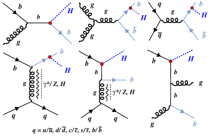
The cross section for processes, involving the production of a Higgs boson and a bottom quark, is of the order of , where represents the Yukawa coupling strength of the b-quark and denotes the strong coupling constant. On the other hand, the higher-order processes that include an additional jet have a cross section of . These processes involve the emission of an extra jet alongside the Higgs boson and bottom quark, resulting in a higher suppression factor due to the additional power of the strong coupling constant.
To gain insights into the impact of varying the coupling modifiers at the LHC, we examine the changes in the signal cross section concerning the SM when is altered by approximately from their SM values. For , the relative change in the cross section is approximately , whereas for , . Additionally, the effect of changing within and of the SM value, results in relative changes of approximately and , respectively.
To assess the effects of the effective couplings on productions in association with a jet, the MadGraph5_aMC@NLO package (version 3.5.1) [50, 51, 52] is utilised. This package allows for the calculation of cross-sections and event generation for various processes. In this case, the effective Lagrangian, as introduced in Eq.3, is implemented in the FeynRule program. The resulting model, known as the Universal FeynRules Output (UFO) model [53], is then provided as input to the MadGraph5_aMC@NLO program. The production of with an additional parton in the final state is considered at leading order, employing relevant matrix elements. The events with zero and one additional parton are combined using the MLM matching scheme [55], which ensures a consistent description of the production process.
In this study, we aim to determine a realistic sensitivity of the +jet process to general coupling, specifically focusing on the and . To achieve this, we carry out the analysis using the Higgs decay channel to two photons, which is known for its well-reconstructed and rather clean signature. This choice allows us to well estimate the background processes and provides valuable insights into the impact of different contributions on and . With Higgs boson decaying into two photons, the final state consists of two photons and at least one jet from which at least one is originating from the hadronization of a b-quark.
The analysis considers several dominant background processes that contribute to the signal. These background processes, which need to be carefully taken into account, include:
-
•
SM production of +jet (merged and +jet using MLM prescription), where Higgs boson decays into and jet can be a light or a heavy flavour jet.
-
•
Higgs boson production from gluon-gluon fusion process: .
-
•
Higgs boson production in association with a vector boson: , where and .
-
•
Di-photon production associated with b-quark jets ().
-
•
Di-photon production associated with c-quark jets (). This background arises from the production of a pair of photon, not coming from Higgs boson, accompanied by c-quark jets, where the c-jets are mis-tagged as b-jets.
-
•
Di-photon production associated with light flavour jets where light flavour jets are misidentified as b-jets.
To ensure sufficient statistics and obtain a more precise estimate of their contributions, the di-photon production associated with different types of jets, including b-quark jets, c-quark jets, and light flavour (non-bottom, non-charm) quark jets, is generated separately in the analysis. By generating these processes independently, it becomes possible to have an adequate number of events for each specific jet flavour and accurately estimate their individual contributions to the di-photon final state. This approach allows for a more comprehensive understanding of the impact of different jet flavors on the di-photon signal and helps in properly accounting for their respective backgrounds in the analysis.
4 Simulation and Analysis Strategy
The SM background processes and signal events are generated using the MadGraph5_aMC@NLO event generator. Specifically, the Higgs boson production in association with a b-quark and a jet sample is obtained by merging the Higgs boson plus b-quark () sample and the Higgs boson plus b-quark plus jet (+jet) sample using the MLM merging prescription. By merging the samples, a comprehensive description of the Higgs boson production in association with a b-quark and a jet is achieved, allowing for accurate modelling and analysis of the signal and background processes.
After generating the samples, they undergo further simulation and modelling to account for various effects. First, the samples are passed through PYTHIA 8.3 [56], which handles parton showering, hadronisation, and the decay of unstable particles. To account for the effects of the detector, the Delphes 3.5.0 package [57] is utilised, which simulates both CMS detector phase II card and the FCC-hh card. Delphes takes the generated particles as input and applies realistic detector response and resolution effects to the particles. For jet reconstruction, the anti- algorithm [58] with a cone size parameter , implemented in the FastJet package [59], is employed. This algorithm clusters particles into jets based on their proximity in the detector. To identify and tag jets originating from b-quarks, b-tagging efficiency and misidentification rates are considered. The efficiency of b-tagging for a jet is and dependent. Additionally, misidentification rates for charm-jets and light-flavour jets are taken into account. For example, for the HL-LHC with CMS Phase II Delphes card, the b-tagging efficiency for a jet with and is set to . The misidentification rate for the charm-jets is dependent and for the light-flavour jets is flat. For a charm-jet with and the misidentification rate is while it is for light-flavour jets independent of and . These rates reflect the likelihood of mistakenly tagging a charm-jet or a light-flavour jet as a b-jet. By incorporating these simulation and modelling steps, the analysis aims to realistically account for detector effects, jet reconstruction, and the identification of b-jets, charm-jets, and light-flavour jets, thereby providing a more accurate description of the experimental observables.
4.1 Events Selection
To identify signal events, specific criteria are applied. The event selection requires the presence of exactly two isolated photons. These photons must have a transverse momentum greater than or equal to 20 GeV and a pseudorapidity within the range of . An isolated photon is defined as one that exhibits minimal activity in its vicinity, reducing the probability of originating from a jet. A small value of the isolation variable indicates a high degree of isolation, implying that the photon is more likely to be a genuine rather than originating from a jet. The isolation of a photon, , is quantified using an isolation variable, which is calculated as the ratio of the sum of transverse momenta () of other particles around the photon to the transverse momentum of the photon itself. For both photons the isolation variable is required to be less than .
Additionally, each event must contain at least one jet, out of which at least one must be identified as b-jets using a b-tagging criterion. The jets (b-jets) are required to have a greater than or equal to 30 GeV and a pseudorapidity within the range of .
To ensure that the selected objects are well-isolated, an angular separation criterion is applied. The angular separation between any two objects (photons or jets) is quantified using the variable , where represents the azimuthal angle and represents the pseudorapidity. The requirement is set at for all possible combinations of objects (photon-photon, photon-jet, and jet-jet). This criterion helps to ensure that the selected objects are sufficiently separated from each other in the detector.
By applying these selection criteria, the analysis aims to isolate signal events that satisfy the specific kinematic and isolation requirements, ensuring the quality and reliability of the data used for further analysis. Table 1 displays the efficiencies of the signal when the coupling is set to 1.05 and the coupling is set to 0.0. It also includes the efficiencies of the main background processes after applying the cuts. The efficiencies represent the fraction of events that pass the selection criteria, for each process.
| Signal | SM | b-jets+ | c-jets+ | light-jets+ | |
|---|---|---|---|---|---|
| HL-LHC | |||||
| FCC-hh |
The cross sections of other background processes such as , and after the selection are found to be negligible in both HL-LHC and FCC-hh. At the end of this section, we address the potential impact of a background arising from the misidentification of jets as photons in multijet and jets+ production. This occurs when jets contain neutral pions that decay into two photons, resulting in overlapping photon showers that appear as a single photon in the detector. To mitigate the QCD multijet background, it is crucial to develop methods to identify and reject jets mimicking photons. This background process has a significantly higher cross section compared to other backgrounds, with a difference spanning several orders of magnitude. However, by applying kinematic requirements (excluding criteria related to photons) and ensuring the presence of only b-jets, the cross section of the multijet and jets+ background is reduced to approximately pb. The probability of a jet being misidentified as a photon depends on the transverse momentum of the fake photon, typically ranging from to depending on fake photons . By imposing a requirement of two photons, the contribution of this background is effectively minimised to a low level. While this analysis neglects the multijet background, it is important to emphasise that a dedicated and more realistic detector simulation is necessary to accurately estimate its potential contribution. Such a simulation should consider the specific characteristics of the experimental setup and incorporate a detailed representation of the detector response. Future studies should address this aspect to provide a more comprehensive assessment of the multijet background’s impact.
4.2 Multivariate analysis
In this analysis, the applied cuts on individual variables are generally loose, meaning they do not significantly suppress a substantial fraction of background events while also reducing the signal events. To achieve a better discrimination between the signal and background processes a multivariate analysis is used [60, 61, 62, 63, 64]. In particular a Boosted Decision Tree (BDT) is trained to increase the sensitivity. All the backgrounds are taken into account during the BDT training, with each background process weighted accordingly. This helps in obtaining an effective separation of signal events from the background events. To enhance sensitivity, separate analyses are conducted for the CP-even and CP-odd signals using distinct BDT test and training sets. This approach allows for a more targeted investigation of each signal, optimizing the discrimination power and enhancing the overall sensitivity of the analysis. Distinct sets of variables for CP-even () and CP-odd () signal processes are employed in the BDT models for analyses at both the HL-LHC and FCC-hh. The included variables are as follows:
-
•
transverse momenta of first and second photon.
-
•
transverse momentum of the most energetic b-jet.
-
•
: the magnitude of the vector sum of the transverse momenta of the two photons.
-
•
: invariant mass of two photons (reconstructed Higgs boson mass).
-
•
: the invariant mass of two photons and the leading b-jet system.
-
•
: the invariant mass of leading photon and leading b-jet system.
-
•
: the invariant mass of second photon and first leading b-jet system.
-
•
: the angular distance between the first and second photon.
-
•
: the cosine of angle between the two photons.
- •
-
•
mean IP of the b-tagged jet defined as:
(6) where and are the transverse impact parameter and the longitudinal impact parameter values of th track inside the b-tagged jet cone with . The total number of tracks inside the jet cone is .
-
•
b-jet charge ():
(7) where the sum is over the particles inside the reconstructed b-jet cone, is the integer charge value of the observed color-neutral object, is the magnitude of its transverse momentum w.r.t the beam axis, and the total transverse momentum of the b-jet is denoted by . More details of the jet charge definition is found Ref.[69].
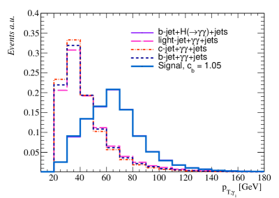
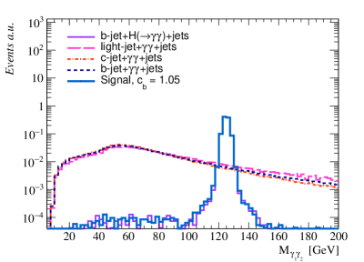
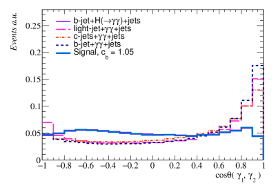
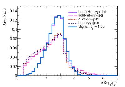
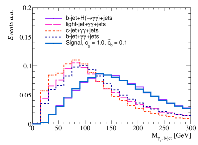
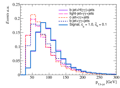
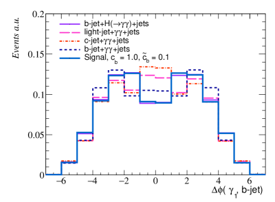
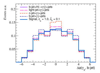
Figure 2 displays the normalised distributions of some the input variables for the CP-even signal. The distributions for signal are for the case . In particular, first photon , invariant mass of diphoton, cosine of the angle between two photons (), and the angular distance between the di-photon system () are depicted in Fig.2. The normalised distributions of some the input variables for the CP-odd case with as for signal events are presented in Fig.3. The invariant mass of the leading photon and the leading jet system, highest b-jet , and the difference between the azimuthal angles of and the of the highest b-jet are shown as examples of the input variables for the CP-odd BDT.
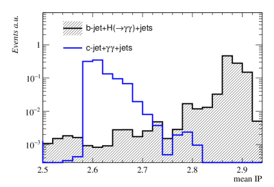
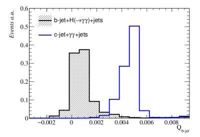
There is a substantial contribution from the c-jet++jets background, primarily arising from the elevated misidentification rate of c-quark jets as b-jets. This misattribution is rooted in the reliance of heavy-flavor jet identification algorithms on variables linked to the characteristics of heavy-flavor hadrons, such as their lifetimes. Notably, heavy-flavor hadrons containing b-quarks exhibit a lifetime on the order of 1.5 ps, whereas c-hadrons have a lifetime of 1 ps or less. Consequently, b hadrons typically display displacements ranging from a few millimeters to one centimeter, depending on their momentum-values that can align with those of energetic jets containing c-hadrons. To discern between backgrounds featuring jets originating from c quarks, we utilize the mean impact parameter and the charge of the identified b-jet as input variables for the BDT. The distribution of these two variables for the b-jet++jets and the c-jet++jets backgrounds is illustrated in Fig.4 for comparative analysis.
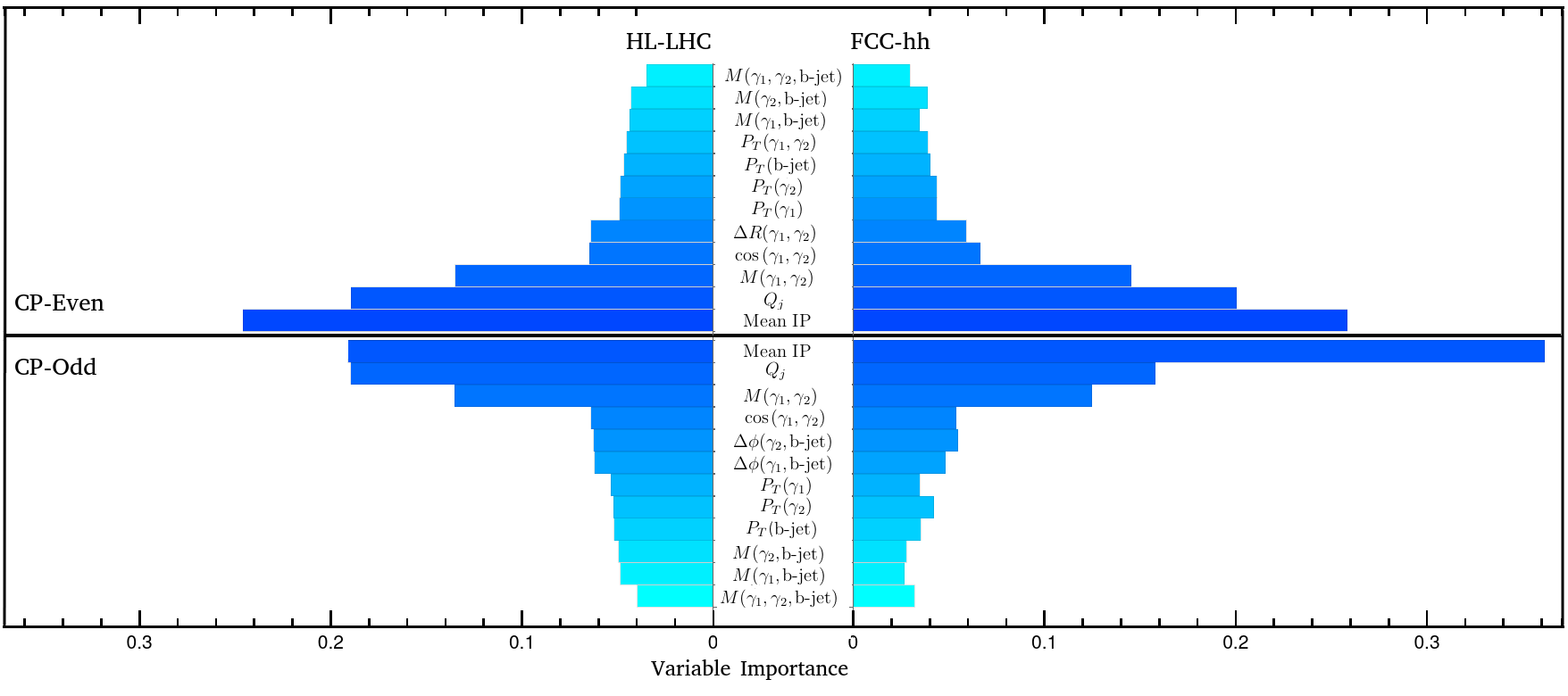
It is notable that there is always room for improvement in the analysis, especially by selecting a more optimal set of variables. However, the variables utilised in our study have proven to be effective discriminators, as evidenced below. We employ the relative importance to filter out the most crucial variables while maintaining the accuracy of the BDT. By utilising the feature importance, we identify and retain the variables that have the highest significance without compromising the overall accuracy of the BDT model. The mean IP, b-jet charge, and the invariant mass of the diphoton system, and the cosine between the two photons angle emerge as the most significant in distinguishing the signal from the backgrounds for both the HL-LHC and FCC-hh. In Figure 5, we present the relative importance of each observable based on the separation between the signal and backgrounds. The ranking is shown for both the HL-LHC and the FCC-hh. The top panel illustrates the relevance of kinematic variables as inputs for the BDT in distinguishing CP-even signals, while the bottom panel focuses on CP-odd signals from the main background processes. The left subplot depicts variable importance for the LHC, and the right subplot presents the corresponding analysis for the FCC-hh.
We proceed with the implementation of the BDT algorithm using the following methodology. The datasets containing independent event samples for both the signal and background are randomly divided into two equal parts. One part is used to train the BDT algorithm, while the other serves as a validation set for both signal and background events.
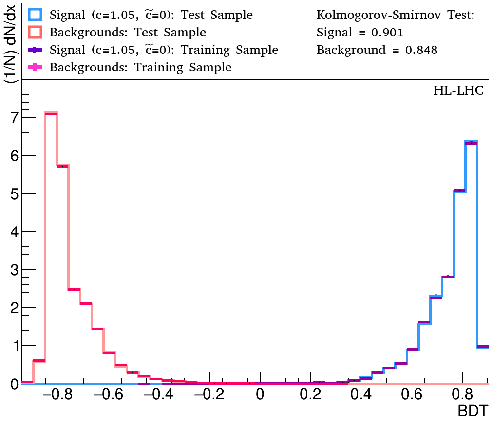
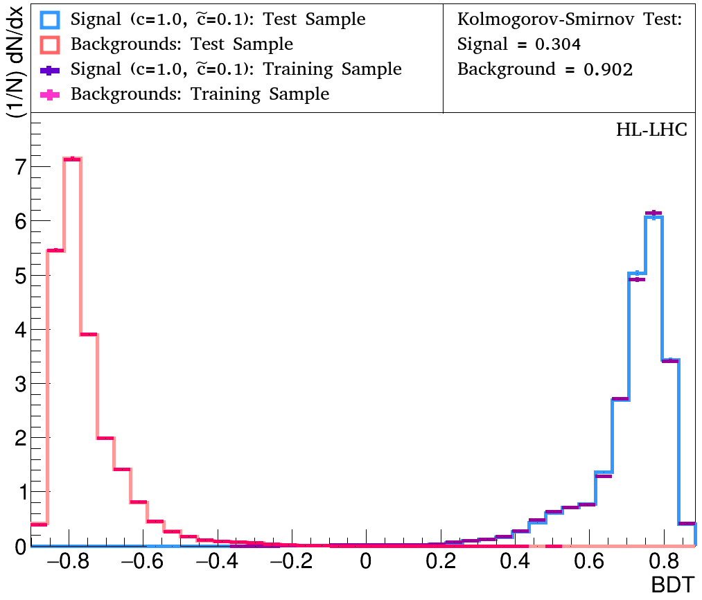
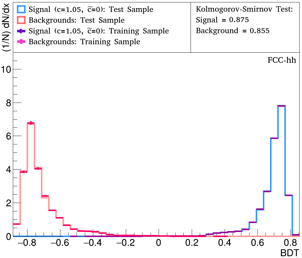
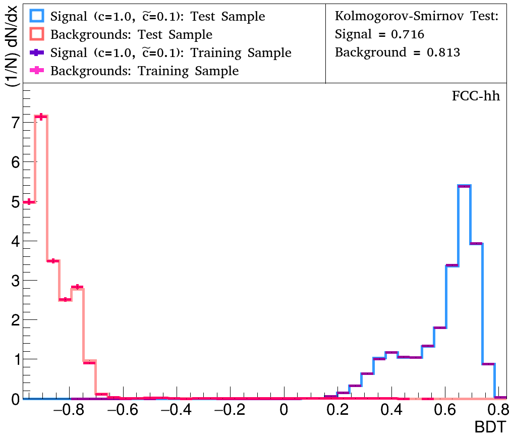
As mentioned earlier, we employ twelve parameters to train the BDT algorithm separately for CP-even and CP-odd. To ensure optimal performance and minimise the risk of overtraining, we take necessary precautions. We have taken explicit measures to prevent overtraining by verifying that the Kolmogorov-Smirnov probability, which measures the similarity between distributions. Figure 6 displays that BDT output distributions for both HL-LHC (top) and FCC-hh (bottom) and illustrates the Kolmogorov-Smirnov probability for both the training and testing samples, demonstrating that neither the signal nor the background samples are overtrained. To optimise sensitivity, we apply an appropriate cut on the BDT response. This cut is determined to maximise the ability to discriminate between the signal and background events. By applying this cut, we obtain the corresponding numbers of signal () and background () events. Using these event counts, we calculate the sensitivity for parameters and .
5 Results
To determine the statistical significance, denoted as , we employ the following formula. Given a number of signal events () and background events () at a specific luminosity (), considering an uncertainty of on background, the significance () is calculated as [70, 71]:
| (8) |
In case that , is reduced to the following formula:
| (9) |
In the limit of large number of background events with respect to signal, . Now, we present the sensitivity reach for both the HL-LHC and the FCC-hh. In Fig.7, the and allowed regions for and are displayed in Table 2 and Fig.7. The integrated luminosity considered for the HL-LHC is 3 ab-1, while for the FCC-hh, it is taken as 15 ab-1. The regions allowed within and are also displayed, accounting for a systematic uncertainty of for background.
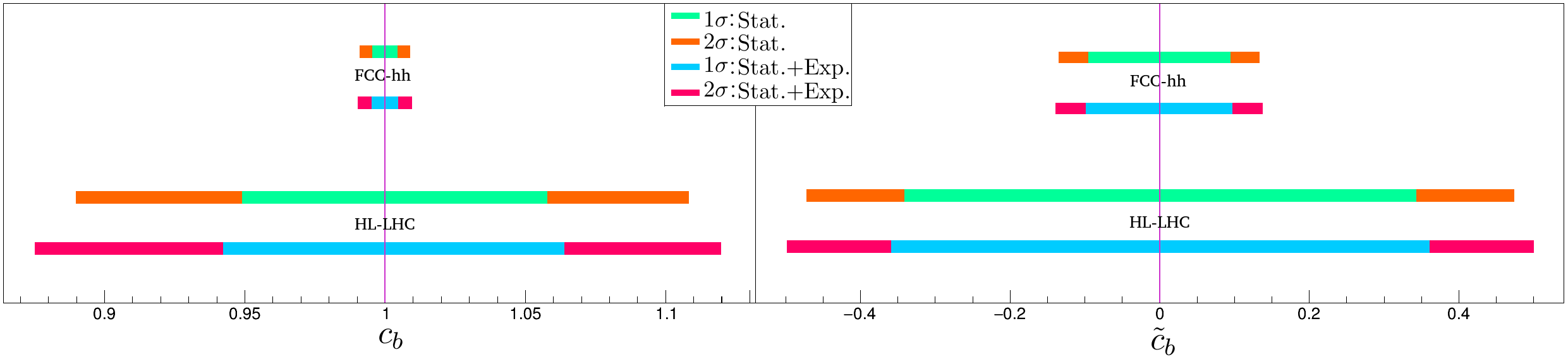
| Uncertainty | HL-LHC | FCC-hh | ||
| 1 | Stat. | |||
| Stat.+Exp. | ||||
| 2 | Stat. | |||
| Stat.+Exp. | ||||
| 1 | Stat. | |||
| Stat.+Exp. | ||||
| 2 | Stat. | |||
| Stat.+Exp. |
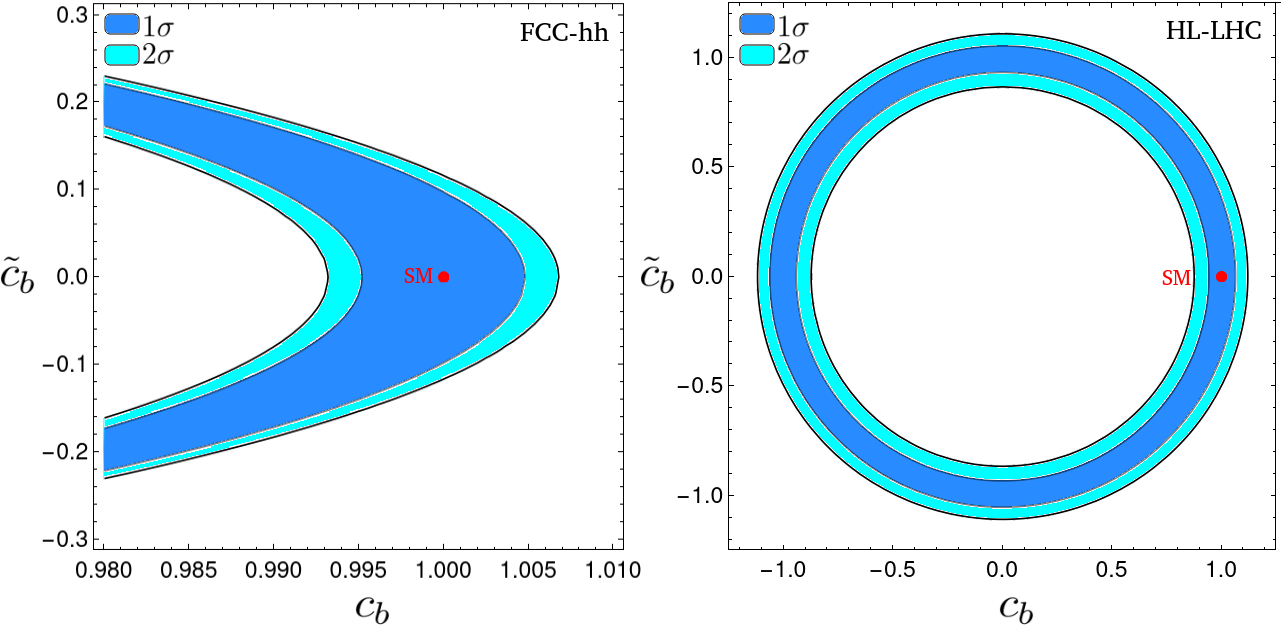
5.1 Bounds on space
Figure 8 illustrates the anticipated exclusion regions within the parameter space for both the HL-LHC and FCC-hh colliders, taking into account integrated luminosities of 3 ab-1 and 15 ab-1, respectively. These exclusion limits were calculated under the assumption that the kinematics of the signal events remain independent of the specific values of the and couplings. Additionally, the presented limits incorporate an overall systematic uncertainty of . Upon comparison, it is evident that the limits experience slight enhancements with the increase in center-of-mass energy from the HL-LHC to the FCC-hh. The parameter space region obtained for the FCC-hh exhibits a circular shape, similar to that for the HL-LHC. However, due to the compactness of the region delineated for the FCC-hh, we opted to zoom in on a restricted area surrounding the SM value. Consequently, this adjustment resulted in an elliptical appearance, facilitating a more refined visualization of the parameter space vicinity to the SM point.
6 Exploration of the CP-odd coupling
In this section, we introduce an asymmetry observable that is sensitive to the magnitude of the pseudo-scalar coupling (). To evaluate this observable, we apply the simulation chain and selection criteria described in Section 4 for various values of the coupling.
The differential production cross section associated to any CP-mixed case of the coupling in H+b+jet signal can be parameterized according to the following:
| (10) |
where , , and are corresponding to the signal differential cross sections for the CP-even, CP-odd couplings and interference terms, respectively. The integration of the interference term in Eq. 10 over the whole phase space disappears because when a CP-even amplitude and a CP-odd amplitude interfere, the resulting interference term oscillates in sign across different regions of phase space and the integral of an odd function over a symmetric interval vanishes. Consequently, the interference term doesn’t add anything to the overall rate or to CP-even measurements like transverse momenta and invariant masses distributions. Instead, it only affects observables designed specifically to measure CP-odd phenomena. We construct an asymmetry observable from the azimuthal angular distributions of the final state objects in process. This observable, , is sensitive to the CP-violating coupling of the interaction. We define the angular asymmetry with respect to the azimuthal angle as:
| (11) |
where
| (12) |
where is defined as the azimuthal angle between the Higgs boson and the highest b-quark in the event, where the Higgs boson is reconstructed from the two photons. According to the general expression provided in Eq.10, we anticipate the following functional form for the asymmetry:
| (13) |
where is the SM case. We note that the denominator represents the total cross section and thus does not contain an interference term. Assuming , the deviation of due to the CP-odd coupling from the SM has the following form:
| (14) |
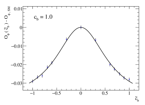
where parameters , , and . To illustrate the sensitivity of the asymmetry, we explore the relationship between the and coupling. Several Monte-Carlo simulated samples consisting of 500K events is analyzed to discern the degree to which the asymmetry is influenced by the presence of the coupling. The difference between the asymmetry and its SM value, , is plotted against at the LHC, as illustrated in Figure 9. In the plot, the value of is fixed at the SM value of and the uncertainty depicted is purely statistical. By conducting a fit, we derive the following result: , and . It is evident from the plot that the exhibits sensitivity to the magnitude of CP-odd coupling. As increases, falls below the SM value. It is noteworthy that receives a minor impact from the interference term because of the very small coefficient of linear term of with respect to the term , i.e. . As a result, the bounds which will be derived on using are expected to exhibit only a minimal degree of asymmetry.
We also investigate the sensitivity of the asymmetry as a probe of CP-violating couplings at the HL-LHC and FCC-hh. To quantify this, all selection criteria presented in section 4.1 are followed. We assess the statistical significance in the measurement of the asymmetry as , where is:
| (15) |
where is the SM cross section and is the integrated luminosity. The signal significance is dependent on and and has the following form:
| (16) |
As our focus lies on the CP-odd coupling, is set to its SM value and we concentrate on . In Figure 10, the and regions of are depicted versus the integrated luminosity for both the HL-LHC and FCC-hh.
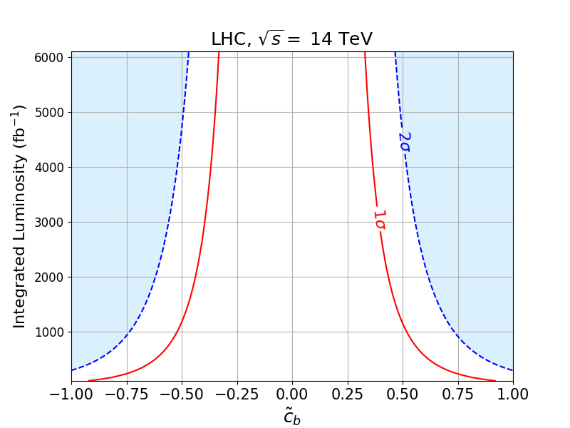
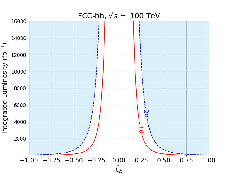
As observed, the () region of is accessible down to with an integrated luminosity of 3000 fb-1 at the HL-LHC and down to with an integrated luminosity of 15000 fb-1 at the FCC-hh.
7 Summary and conclusions
This study focused on investigating the sensitivity of the process at the HL-LHC and FCC-hh colliders in order to explore the CP-even and CP-odd couplings of . The analysis involved constraining the new physics couplings, and , by conducting a search through the channel and studying the subsequent decay of the Higgs boson into two photons. Monte Carlo event generation was employed to simulate the signal and relevant background processes, and detector effects were taken into account. To distinguish the signal from the background, a carefully selected set of discriminating variables was analysed using a multivariate technique, in particular, by employing Boosted Decision Trees (BDTs). The expected and limits on and were obtained, and the exclusion region in the - plane were determined. These limits correspond to integrated luminosities of 3 ab-1 and 15 ab-1 for the HL-LHC and FCC-hh, respectively.
Comparing the obtained limits with the current experimental bounds, it was found that a significant portion of the unexplored - parameter space could be accessed through this analysis. By assuming one non-zero coupling at a time for comparison, the coupling was found to range from based on the LHC Higgs signal strength data at confidence level (CL). The direct predicted ranges from this study were for the HL-LHC and for the FCC-hh.
Regarding the parameter, the current limits were within the range based on the LHC Higgs signal strength data and from electron EDM at CL. The direct measurement from this analysis excluded the range for the HL-LHC and for the FCC-hh at the level. Both the HL-LHC and FCC-hh demonstrated the potential to provide limits on and at the same order of magnitude as or even better than those obtained from indirect bounds.
We also introduced a novel asymmetry tailored to investigate CP violation within the coupling, applying exclusively lab-frame momenta. Our analysis underscored the effectiveness of this asymmetry in constraining the CP-odd couplings of the bottom quark Yukawa couplings.
Upon contrasting the findings of this study, it becomes apparent that the process emerges as a powerful and direct avenue for investigating both the CP-even and CP-odd aspects of the interactions at proton-proton colliders. This efficacy is primarily attributed to the incorporation of a more extensive final state. There are potential avenues to improve the results. Firstly, incorporating complete next-to-leading order predictions for the process, including loop level diagrams, can yield more accurate and reliable outcomes. Secondly, to enhance sensitivity and statistical significance, the inclusion of additional decay modes of the Higgs boson, such as and needs to be considered.
Acknowledgement
The authors would like to thank M. Ebrahimi for her fruitful discussions in multivariate analysis algorithms and M. Zaro for his valuable guidances in generating events with MadGraph.
References
- [1] M. Aaboud et al. [ATLAS], Phys. Lett. B 786, 59-86 (2018) doi:10.1016/j.physletb.2018.09.013 [arXiv:1808.08238 [hep-ex]].
- [2] A. M. Sirunyan et al. [CMS], Phys. Rev. Lett. 121, no.12, 121801 (2018) doi:10.1103/PhysRevLett.121.121801 [arXiv:1808.08242 [hep-ex]].
- [3] G. Aad et al. [ATLAS], Eur. Phys. J. C 81, no.2, 178 (2021) doi:10.1140/epjc/s10052-020-08677-2 [arXiv:2007.02873 [hep-ex]].
- [4] The CMS Collaboration [CMS], CMS-PAS-FTR-18-011.
- [5] Y. Heo, D. W. Jung and J. S. Lee, [arXiv:2402.02822 [hep-ph]].
- [6] S. Heinemeyer et al. [LHC Higgs Cross Section Working Group], doi:10.5170/CERN-2013-004 [arXiv:1307.1347 [hep-ph]].
- [7] A. Tumasyan et al. [CMS], Nature 607, no.7917, 60-68 (2022) doi:10.1038/s41586-022-04892-x [arXiv:2207.00043 [hep-ex]].
- [8] M. Cepeda, S. Gori, P. Ilten, M. Kado, F. Riva, R. Abdul Khalek, A. Aboubrahim, J. Alimena, S. Alioli and A. Alves, et al. CERN Yellow Rep. Monogr. 7, 221-584 (2019) doi:10.23731/CYRM-2019-007.221 [arXiv:1902.00134 [hep-ph]].
- [9] A. Crivellin, [arXiv:2304.01694 [hep-ph]].
- [10] K. G. Wilson, Rev. Mod. Phys. 55, 583-600 (1983) doi:10.1103/RevModPhys.55.583
- [11] T. Appelquist and J. Carazzone, Phys. Rev. D 11, 2856 (1975) doi:10.1103/PhysRevD.11.2856
- [12] W. Buchmuller and D. Wyler, Nucl. Phys. B 268, 621-653 (1986) doi:10.1016/0550-3213(86)90262-2
- [13] B. Grzadkowski, M. Iskrzynski, M. Misiak and J. Rosiek, JHEP 10, 085 (2010) doi:10.1007/JHEP10(2010)085 [arXiv:1008.4884 [hep-ph]].
- [14] K. Hagiwara, S. Ishihara, R. Szalapski and D. Zeppenfeld, Phys. Rev. D 48, 2182-2203 (1993) doi:10.1103/PhysRevD.48.2182
- [15] C. N. Leung, S. T. Love and S. Rao, Z. Phys. C 31, 433 (1986) doi:10.1007/BF01588041
- [16] M. B. Einhorn and J. Wudka, Nucl. Phys. B 876, 556-574 (2013) doi:10.1016/j.nuclphysb.2013.08.023 [arXiv:1307.0478 [hep-ph]].
- [17] S. Willenbrock and C. Zhang, Ann. Rev. Nucl. Part. Sci. 64, 83-100 (2014) doi:10.1146/annurev-nucl-102313-025623 [arXiv:1401.0470 [hep-ph]].
- [18] R. Contino, M. Ghezzi, C. Grojean, M. Muhlleitner and M. Spira, JHEP 07, 035 (2013) doi:10.1007/JHEP07(2013)035 [arXiv:1303.3876 [hep-ph]].
- [19] S. Bar-Shalom, A. Soni and J. Wudka, Phys. Rev. D 92, no.1, 015018 (2015) doi:10.1103/PhysRevD.92.015018 [arXiv:1405.2924 [hep-ph]].
- [20] R. S. Gupta, A. Pomarol and F. Riva, Phys. Rev. D 91, no.3, 035001 (2015) doi:10.1103/PhysRevD.91.035001 [arXiv:1405.0181 [hep-ph]].
- [21] A. Alloul, B. Fuks and V. Sanz, JHEP 04, 110 (2014) doi:10.1007/JHEP04(2014)110 [arXiv:1310.5150 [hep-ph]].
- [22] F. Bishara, P. Englert, C. Grojean, G. Panico and A. N. Rossia, JHEP 06, 077 (2023) doi:10.1007/JHEP06(2023)077 [arXiv:2208.11134 [hep-ph]].
- [23] H. Bahl, E. Fuchs, S. Heinemeyer, J. Katzy, M. Menen, K. Peters, M. Saimpert and G. Weiglein, Eur. Phys. J. C 82, no.7, 604 (2022) doi:10.1140/epjc/s10052-022-10528-1 [arXiv:2202.11753 [hep-ph]].
- [24] J. Brod, J. M. Cornell, D. Skodras and E. Stamou, JHEP 08, 294 (2022) doi:10.1007/JHEP08(2022)294 [arXiv:2203.03736 [hep-ph]].
- [25] A. Djouadi and G. Moreau, Eur. Phys. J. C 73, no.9, 2512 (2013) doi:10.1140/epjc/s10052-013-2512-9 [arXiv:1303.6591 [hep-ph]].
- [26] R. Harnik, A. Martin, T. Okui, R. Primulando and F. Yu, Phys. Rev. D 88, no.7, 076009 (2013) doi:10.1103/PhysRevD.88.076009 [arXiv:1308.1094 [hep-ph]].
- [27] F. Bishara, Y. Grossman, R. Harnik, D. J. Robinson, J. Shu and J. Zupan, JHEP 04, 084 (2014) doi:10.1007/JHEP04(2014)084 [arXiv:1312.2955 [hep-ph]].
- [28] F. Demartin, B. Maier, F. Maltoni, K. Mawatari and M. Zaro, Eur. Phys. J. C 77, no.1, 34 (2017) doi:10.1140/epjc/s10052-017-4601-7 [arXiv:1607.05862 [hep-ph]].
- [29] H. Bahl and S. Brass, JHEP 03, 017 (2022) doi:10.1007/JHEP03(2022)017 [arXiv:2110.10177 [hep-ph]].
- [30] H. Bahl, P. Bechtle, S. Heinemeyer, J. Katzy, T. Klingl, K. Peters, M. Saimpert, T. Stefaniak and G. Weiglein, JHEP 11, 127 (2020) doi:10.1007/JHEP11(2020)127 [arXiv:2007.08542 [hep-ph]].
- [31] J. Ellis, V. Sanz and T. You, JHEP 07, 036 (2014) doi:10.1007/JHEP07(2014)036 [arXiv:1404.3667 [hep-ph]].
- [32] T. Corbett, O. J. P. Eboli, J. Gonzalez-Fraile and M. C. Gonzalez-Garcia, Phys. Rev. D 86, 075013 (2012) doi:10.1103/PhysRevD.86.075013 [arXiv:1207.1344 [hep-ph]].
- [33] J. Ellis, V. Sanz and T. You, JHEP 03, 157 (2015) doi:10.1007/JHEP03(2015)157 [arXiv:1410.7703 [hep-ph]].
- [34] C. Englert, Y. Soreq and M. Spannowsky, JHEP 05, 145 (2015) doi:10.1007/JHEP05(2015)145 [arXiv:1410.5440 [hep-ph]].
- [35] C. Englert and M. Spannowsky, Phys. Lett. B 740, 8-15 (2015) doi:10.1016/j.physletb.2014.11.035 [arXiv:1408.5147 [hep-ph]].
- [36] J. A. Aguilar-Saavedra, J. M. Cano and J. M. No, Phys. Rev. D 103, no.9, 095023 (2021) doi:10.1103/PhysRevD.103.095023 [arXiv:2008.12538 [hep-ph]].
- [37] T. Biswas and A. Datta, JHEP 05, 104 (2023) doi:10.1007/JHEP05(2023)104 [arXiv:2208.08432 [hep-ph]].
- [38] B. Carlson, T. Han and S. C. I. Leung, Phys. Rev. D 104, no.7, 073006 (2021) doi:10.1103/PhysRevD.104.073006 [arXiv:2105.08738 [hep-ph]].
- [39] S. Khatibi and M. Mohammadi Najafabadi, Phys. Rev. D 90, no. 7, 074014 (2014) doi:10.1103/PhysRevD.90.074014 [arXiv:1409.6553 [hep-ph]].
- [40] H. Khanpour, S. Khatibi and M. Mohammadi Najafabadi, “Probing Higgs boson couplings in H+ production at the LHC,” Phys. Lett. B 773, 462 (2017) doi:10.1016/j.physletb.2017.09.005 [arXiv:1702.05753 [hep-ph]].
- [41] G. Haghighat, R. Jafari, H. Khanpour and M. Mohammadi Najafabadi, [arXiv:2305.05462 [hep-ph]].
- [42] J. de Blas, M. Cepeda, J. D’Hondt, R. K. Ellis, C. Grojean, B. Heinemann, F. Maltoni, A. Nisati, E. Petit and R. Rattazzi, et al. JHEP 01, 139 (2020) doi:10.1007/JHEP01(2020)139 [arXiv:1905.03764 [hep-ph]].
- [43] E. Fuchs, M. Losada, Y. Nir and Y. Viernik, JHEP 05, 056 (2020) doi:10.1007/JHEP05(2020)056 [arXiv:2003.00099 [hep-ph]].
- [44] C. Grojean, A. Paul and Z. Qian, JHEP 04, 139 (2021) doi:10.1007/JHEP04(2021)139 [arXiv:2011.13945 [hep-ph]].
- [45] P. Konar, B. Mukhopadhyaya, R. Rahaman and R. K. Singh, Phys. Lett. B 818, 136358 (2021) doi:10.1016/j.physletb.2021.136358 [arXiv:2101.10683 [hep-ph]].
- [46] F. Bordry, M. Benedikt, O. Brüning, J. Jowett, L. Rossi, D. Schulte, S. Stapnes and F. Zimmermann, [arXiv:1810.13022 [physics.acc-ph]].
- [47] C. Adolphsen, D. Angal-Kalinin, T. Arndt, M. Arnold, R. Assmann, B. Auchmann, K. Aulenbacher, A. Ballarino, B. Baudouy and P. Baudrenghien, et al. CERN Yellow Rep. Monogr. 1, 1-270 (2022) doi:10.23731/CYRM-2022-001 [arXiv:2201.07895 [physics.acc-ph]].
- [48] V. Andreev et al. [ACME], Nature 562, no.7727, 355-360 (2018) doi:10.1038/s41586-018-0599-8
- [49] P. Artoisenet, P. de Aquino, F. Demartin, R. Frederix, S. Frixione, F. Maltoni, M. K. Mandal, P. Mathews, K. Mawatari and V. Ravindran, et al. JHEP 11, 043 (2013) doi:10.1007/JHEP11(2013)043 [arXiv:1306.6464 [hep-ph]].
- [50] J. Alwall, M. Herquet, F. Maltoni, O. Mattelaer and T. Stelzer, “MadGraph 5 : Going Beyond,” JHEP 1106, 128 (2011) doi:10.1007/JHEP06(2011)128 [arXiv:1106.0522 [hep-ph]].
- [51] J. Alwall, C. Duhr, B. Fuks, O. Mattelaer, D. G. Ozturk and C. H. Shen, “Computing decay rates for new physics theories with FeynRules and MadGraph 5_aMC@NLO,” Comput. Phys. Commun. 197, 312 (2015) doi:10.1016/j.cpc.2015.08.031 [arXiv:1402.1178 [hep-ph]].
- [52] J. Alwall et al., “The automated computation of tree-level and next-to-leading order differential cross sections, and their matching to parton shower simulations,” JHEP 1407, 079 (2014) doi:10.1007/JHEP07(2014)079 [arXiv:1405.0301 [hep-ph]].
- [53] A. Alloul, N. D. Christensen, C. Degrande, C. Duhr and B. Fuks, “FeynRules 2.0 - A complete toolbox for tree-level phenomenology,” Comput. Phys. Commun. 185, 2250 (2014) doi:10.1016/j.cpc.2014.04.012 [arXiv:1310.1921 [hep-ph]].
- [54] C. Degrande, C. Duhr, B. Fuks, D. Grellscheid, O. Mattelaer and T. Reiter, “UFO - The Universal FeynRules Output,” Comput. Phys. Commun. 183, 1201 (2012) doi:10.1016/j.cpc.2012.01.022 [arXiv:1108.2040 [hep-ph]].
- [55] M. L. Mangano, M. Moretti, F. Piccinini and M. Treccani, “Matching matrix elements and shower evolution for top-quark production in hadronic collisions,” JHEP 0701, 013 (2007) doi:10.1088/1126-6708/2007/01/013 [hep-ph/0611129].
- [56] T. Sjostrand et al., “An Introduction to PYTHIA 8.2,” Comput. Phys. Commun. 191, 159 (2015) doi:10.1016/j.cpc.2015.01.024 [arXiv:1410.3012 [hep-ph]].
- [57] J. de Favereau et al. [DELPHES 3 Collaboration], “DELPHES 3, A modular framework for fast simulation of a generic collider experiment,” JHEP 1402, 057 (2014) doi:10.1007/JHEP02(2014)057 [arXiv:1307.6346 [hep-ex]].
- [58] M. Cacciari, G. P. Salam and G. Soyez, “The anti- jet clustering algorithm,” JHEP 0804, 063 (2008) doi:10.1088/1126-6708/2008/04/063 [arXiv:0802.1189 [hep-ph]].
- [59] M. Cacciari, G. P. Salam and G. Soyez, “FastJet User Manual,” Eur. Phys. J. C 72, 1896 (2012) doi:10.1140/epjc/s10052-012-1896-2 [arXiv:1111.6097 [hep-ph]].
- [60] A. Hocker et al., “TMVA - Toolkit for Multivariate Data Analysis,” PoS ACAT , 040 (2007) [physics/0703039 [PHYSICS]].
- [61] J. Stelzer, A. Hocker, P. Speckmayer and H. Voss, “Current developments in TMVA: An outlook to TMVA4,” PoS ACAT 08, 063 (2008).
- [62] J. Therhaag [TMVA Core Developer Team Collaboration], “TMVA: Toolkit for multivariate data analysis,” AIP Conf. Proc. 1504, 1013 (2009).
- [63] P. Speckmayer, A. Hocker, J. Stelzer and H. Voss, “The toolkit for multivariate data analysis, TMVA 4,” J. Phys. Conf. Ser. 219, 032057 (2010).
- [64] J. Therhaag, “TMVA Toolkit for multivariate data analysis in ROOT,” PoS ICHEP 2010, 510 (2010).
- [65] C. Englert, P. Galler, A. Pilkington and M. Spannowsky, Phys. Rev. D 99, no.9, 095007 (2019) doi:10.1103/PhysRevD.99.095007 [arXiv:1901.05982 [hep-ph]].
- [66] N. Mileo, K. Kiers, A. Szynkman, D. Crane and E. Gegner, JHEP 07, 056 (2016) doi:10.1007/JHEP07(2016)056 [arXiv:1603.03632 [hep-ph]].
- [67] S. D. Rindani, P. Sharma and A. Shivaji, Phys. Lett. B 761, 25-30 (2016) doi:10.1016/j.physletb.2016.08.002 [arXiv:1605.03806 [hep-ph]].
- [68] F. Boudjema, R. M. Godbole, D. Guadagnoli and K. A. Mohan, Phys. Rev. D 92, no.1, 015019 (2015) doi:10.1103/PhysRevD.92.015019 [arXiv:1501.03157 [hep-ph]].
- [69] D. Krohn, M. D. Schwartz, T. Lin and W. J. Waalewijn, Phys. Rev. Lett. 110, no.21, 212001 (2013) doi:10.1103/PhysRevLett.110.212001 [arXiv:1209.2421 [hep-ph]].
- [70] G. Cowan, K. Cranmer, E. Gross and O. Vitells, Eur. Phys. J. C 71, 1554 (2011) [erratum: Eur. Phys. J. C 73, 2501 (2013)] doi:10.1140/epjc/s10052-011-1554-0 [arXiv:1007.1727 [physics.data-an]].
- [71] R. D. Cousins, J. T. Linnemann and J. Tucker, Nucl. Instrum. Meth. A 595, no.2, 480-501 (2008) doi:10.1016/j.nima.2008.07.086 [arXiv:physics/0702156 [physics.data-an]].