Fast Online Movement Optimization of Aerial Base Stations Based on Global Connectivity Map

Abstract

Unmanned aerial vehicles (UAVs) can serve as aerial base stations (ABSs) to provide wireless connectivity for ground users (GUs) in diverse scenarios. However, it is an NP-hard problem with exponential complexity in $M$ and $N$, in order to maximize the coverage rate (CR) of $M$ GUs by jointly placing $N$ ABSs with limited coverage range. This problem becomes even more intricate when the coverage range becomes irregular due to site-specific obstructions (e.g., buildings) on the air-ground channel, and/or when the GUs are in motion. To address the above challenges, we study a multi-ABS movement optimization problem to maximize the average coverage rate of mobile GUs within a site-specific environment. We tackle this challenging problem by 1) constructing the global connectivity map (GCM) which contains the connectivity information between given pairs of ABS/GU locations; 2) partitioning the ABS movement problem into ABS placement sub-problems and formulate each sub-problem into a binary integer linear programing (BILP) problem based on GCM; 3) proposing a fast online algorithm to execute (one-pass) projected stochastic subgradient descent within the dual space to rapidly solve the BILP problem with near-optimal performance. Numerical results demonstrate that our proposed algorithm achieves a high CR performance close to that obtained by the open source solver (SCIP), yet with significantly reduced running time. In addition, the algorithm also notably outperforms one of the state-of-the-art deep reinforcement learning (DRL) methods and the K-means initiated evolutionary algorithm in terms of CR performance and/or time efficiency.

I Introduction

Unmanned aerial vehicles (UAVs) have attracted increasing attention in civilian domains due to their enhanced mobility and decreasing costs in recent years. In particular, integrating UAVs into wireless communication networks as aerial base stations (ABSs) has been recognized as a promising technology [1]. A pivotal challenge here lies in determining the suitable placement of $N$ ABSs with restricted coverage ranges to attain maximum coverage for $M$ (static) ground users (GUs) [2, 3]. This problem is recognized as an NP-hard problem with exponential complexity in $M$ and $N$ [2]. Specifically, a myriad of algorithms have been proposed to address this problem including the spiral algorithm [2], K-means algorithm [3], and a user-majority-based adaptive UAV deployment approach [4]. These algorithms typically assume the presence of a dominant line-of-sight (LoS) or probabilistic LoS/non-LoS (NLoS) channel model [5], whereby each ABS has a uniform coverage range. Nonetheless, owing to site-specific obstructions (e.g., buildings), the above channel models might fail to depict the intricate LoS or NLoS propagation characteristics at specific ABS and GU positions [6]. For instance, a minor adjustment in the ABS position can lead to a transition from LoS to NLoS propagation towards the GU due to building edges. This affects the ABS-GU channel significantly and increases complexity of the problem.

Some efforts have been made using DRL methods to solve site-specific ABS movement optimization [7]. However, DRL-based methods require careful state-action-reward design, and become more difficult to converge due to the curse of dimensionality and non-stationarity of the environment. Moreover, an enormous and irregular state space for all pairs of possible ABS-GU locations is generated from site-specific LoS/NLoS propagation in the three-dimensional (3D) space, thus imposing high time complexity to find desired ABS locations. Worse still, network dynamics due to GU mobility impose further challenges for the learning/adaption of ABS movement within a short time.

To circumvent the above difficulties, we explore an alternative approach based on radio map instead of DRL. Radio map [6] is used to represent site-specific spatial distribution of average received power radiated from given transmitting source(s), whereby recent advances [8, 9] have provided efficient approaches to construct radio map. The author in [8] proposes an update mechanism based on the amount of wireless environmental changes from image data, combined with the Siamese neural network and an attention mechanism in computer vision to effectively update the radio map. Moreover, an efficient and highly accurate method called RadioUNet [9] is designed for estimating the propagation path loss between transmitters and receivers in site-specific environments.

In this paper, we leverage radio map to solve our problem. First, a global connectivity map (GCM) is introduced, which is a binary matrix containing the connectivity information of given pairs of ABS/GU locations in a site-specific environment. Second, the ABS movement problem is partitioned into a series of ABS placement sub-problems, each aiming to maximize the coverage rate (CR) of all GUs in a short time period subject to ABS movement constraints. Third, each ABS placement subproblem is then formulated as a binary integer linear programing (BILP) problem based on GCM, for which a novel fast online algorithm [10] is introduced with tailored modifications to fit the problem. More specifically, We narrow down the search range by considering the ABS mobility model, which helps reduce the computational complexity of the algorithm. Optimality bounds are also provided for the proposed algorithm. Finally, numerical results demonstrate that our propose algorithm achieves a high CR performance close to that obtained by the open source solver (SCIP)[11], yet with significantly reduced running time. Moreover, superior performance of our algorithm is also observed compared with one of the state-of-the-art DRL methods (TD3) [12] and the K-means initiated evolutionary algorithm (EA) in terms of CR and/or time efficiency.

II System Model and Problem Formulation

Consider a UAV-aided communication system with $N$ UAV-mounted ABSs to serve a group of $M$ mobile GUs in a $D_{1}\times D_{2}$ m² rectangular area with site-specific blockages, as illustrated in Fig. 1. For the purpose of exposition, the blockages are exemplified using a collection of $L$ building blocks (BBs), each with a $D_{w}\times D_{w}$ m² square projection shape and a random height $h_{w}[l]$, $l\in\mathcal{L}\triangleq\{1,\dots,L\}$. In this work, we concentrate on the access network where ABSs aim to provide data communication coverage for GUs, and assume for simplicity that there exists a backhaul network among ABSs.

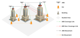
Figure 1: ABS movement optimization to cover mobile GUs in an environment with site-specific blockages.

II-A Discretized ABS/GU Plane

Fixed altitude at height $H$, for the ABS plane, we consider a $D_{1}\times D_{2}$ area partitioned into $K_{1}\times K_{2}$ grids. Denote the ABS plane area as $\boldsymbol{\mathcal{A}}$, the grid area as $\mathcal{A}_{ij}$, $\boldsymbol{\mathcal{A}}\triangleq\cup\mathcal{A}_{ij}$, $i=1,2,\ldots,K_{1},j=1,2,\ldots,K_{2}$. Each grid has length $\alpha_{1}\triangleq\frac{D_{1}}{K_{1}}$, $\alpha_{2}\triangleq\frac{D_{2}}{K_{2}}$, and grid center location is $\boldsymbol{a}_{ij}\triangleq\left(\left(i-\frac{1}{2}\right)\alpha_{1},\left(j-\frac{1}{2}\right)\alpha_{2},H\right),i=1,2,\ldots,K_{1},j=1,2,\ldots,K_{2}$. For simplicity, we assume ABSs always locate at the grid center which make up a set $\boldsymbol{A}$, $\boldsymbol{A}\triangleq\left\{\boldsymbol{a}_{ij}\mid i=1,2,\ldots,K_{1},j=1,2,\ldots,K_{2}\right\}$. For the GU plane, we consider a $D_{1}\times D_{2}$ area partitioned into $K_{1}^{{}^{\prime}}\times K_{2}^{{}^{\prime}}$ grids on the ground. Denote the GU plane area as $\boldsymbol{\mathcal{B}}$, the grid area as $\mathcal{B}_{i^{\prime}j^{\prime}}$, $\boldsymbol{\mathcal{B}}\triangleq\cup\mathcal{B}_{i^{\prime}j^{\prime}},i^{\prime}=1,2,\ldots,K_{1}{}^{\prime},j^{\prime}=1,2,\ldots,K_{2}{}^{\prime}$. Each grid has length $\alpha_{1}{}^{\prime}\triangleq\frac{D_{1}}{K_{1}{}^{\prime}},\alpha_{2}{}^{\prime}\triangleq\frac{D_{2}}{K_{2}{}^{\prime}}$, and grid center location is $\boldsymbol{b}_{i^{\prime}j^{\prime}}\triangleq\left(\left(i^{\prime}-\frac{1}{2}\right)\alpha_{1}{}^{\prime},\left(j^{\prime}-\frac{1}{2}\right)\alpha_{2}{}^{\prime},0\right),i^{\prime}=1,2,\ldots,K_{1}{}^{\prime},j^{\prime}=1,2,\ldots,K_{2}{}^{\prime}$. The grid center in GU plane make up a set $\boldsymbol{B}$, $\boldsymbol{B}\triangleq\left\{\boldsymbol{b}_{i^{\prime}j^{\prime}}\mid i^{\prime}=1,2,\ldots,K_{1}{}^{\prime},j^{\prime}=1,2,\ldots,K_{2}{}^{\prime}\right\}$. The discretized ABS and GU planes are as illustrated in Fig. 2 .

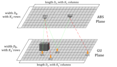
Figure 2: Discretized ABS/GU plane.

II-B ABS/GU Mobility Model

Consider a typical ABS movement trial with a duration of $\Delta T$ s, which is discretized into $I$ equal-length time steps, each lasting $\Delta\tau=\Delta T/I$. For simplicity, we suppose that ABSs fly at a fixed altitude of $H$ m, and GUs move on the ground with a hand-held height of $h_{q}$ m. Furthermore, assume that GUs move at a constant pace of $V_{q}$ m/s but with a random direction at each step. We suppose that the positions of GUs at each step are known and communicated through separate control links to a central planning agent. This planning agent could be located on one of the UAVs or at a ground vehicle station. Denote $\boldsymbol{p}^{(i)}[n]=(x^{(i)}_{p}[n],y^{(i)}_{p}[n])$ as the horizontal position of ABS $n\in\mathcal{N}\triangleq\{1,\dots,N\}$ at step $i\in\mathcal{I}\triangleq\{1,\dots,I\}$. Similarly, denote $\boldsymbol{q}^{(i)}[m]=(x^{(i)}_{q}[m],y^{(i)}_{q}[m])$ as the horizontal position of GU $m\in\mathcal{M}\triangleq\{1,\dots,M\}$ at step $i\in\mathcal{I}$. Denote $\mathcal{P}^{(i)}\triangleq\{\boldsymbol{p}^{(i)}[n]|n\in\mathcal{N}\}$ or $\mathcal{Q}^{(i)}\triangleq\{\boldsymbol{q}^{(i)}[m]|m\in\mathcal{M}\}$ as the location set at step $i\in\mathcal{I}$ for ABSs or GUs, respectively.

Assume each ABS can independently adjust its moving speed as required, subject to a maximum speed constraint of $V^{\max}_{p}$ m/s. Denote $\|\cdot\|$ as the Euclidean norm. Then, the ABS positions in consecutive time steps are restricted by the maximum moving distance, i.e.,

$$\lVert\boldsymbol{p}^{(i)}[n]-\boldsymbol{p}^{(i-1)}[n]\rVert\leq V^{\max}_{p}\cdot\Delta\tau,\forall i\in\mathcal{I},n\in\mathcal{N}.$$ (1)

Moreover, we focus on the outdoor scenario within a bounded area. Denote $\mathcal{C}\subset\mathcal{A}$ as the region occupied by obstacles. The following constraint is thus imposed, i.e.,

$$\boldsymbol{p}^{(i)}[n]\in\mathcal{A}\setminus\mathcal{C},\forall i\in\mathcal{I},n\in\mathcal{N}.$$ (2)

II-C Site-Specific LoS/NLoS Channel Model

Consider downlink communication from ABSs to GUs, while our method can also be applied to uplink communication similarly. To focus on the coverage performance, for simplicity, we assume that the available spectrum is equally partitioned into $M$ orthogonal channels. Each channel is exclusively allocated to an individual GU, thus eliminating intra- or inter-cell interference. Moreover, suppose that each ABS or GU is equipped with omni-directional antenna of unit gain. Assume that each ABS transmits with power $P$ Watt (W) to the corresponding served GU, and the receiver noise power is denoted by $\sigma^{2}$ W. The signal-to-noise ratio (SNR) received by GU $m$ from ABS $n$ can be expressed as

$$\gamma_{m,n}\triangleq g_{m,n}P/\sigma^{2},$$ (3)

where $g_{m,n}\triangleq\bar{g}_{m,n}\xi_{m,n}$ denotes the instantaneous channel power gain, with $\bar{g}_{m,n}$ representing the average channel power and $\xi_{m,n}$ accounting for small scale fading with unit average power. To focus on large scale coverage performance, we assume that the small scale fading effect is averaged out, and concentrate on the dominant LoS and NLoS path-loss constituents, as demonstrated in [5]. A GU $m$ is considered covered by ABS $n$, if the average SNR $\bar{\gamma}_{m,n}\triangleq\bar{g}_{m,n}P/\sigma^{2}$ exceeds or equals a given threshold $\bar{\gamma}$, which corresponds to a threshold of average channel power $\bar{g}\triangleq\bar{\gamma}\sigma^{2}/P$.

Due to site-specific blockages, the ABS-GU channel could be in either LoS or NLoS propagation condition depending on the presence of obstacles in between. For a specific link connecting an ABS at location $\boldsymbol{p}$ and a GU at location $\boldsymbol{q}$, the average channel power gain can be expressed as

$$\bar{g}\triangleq\begin{cases}\bar{g}_{\textrm{L}}(\boldsymbol{p},\boldsymbol{q}),&\quad\textrm{without obstacles in between;}\\ \bar{g}_{\textrm{NL}}(\boldsymbol{p},\boldsymbol{q}),&\quad\textrm{otherwise,}\end{cases}$$ (4)

where $\bar{g}_{\textrm{L}}$ and $\bar{g}_{\textrm{NL}}$ represent the average channel power gains of the LoS and NLoS channels, correspondingly. These can be measured on site by averaging over an adequate number of fading samples, following a procedure similar to that in [13].

II-D Global Connectivity Map and Problem Formulation

In this section, we construct GCM to formulate the considered problem into a BILP problem. Define $u\triangleq(i-1)K_{2}+j$, $i=1,2,\ldots,K_{1}$, $j=1,2,\ldots,K_{2}$ as the flattened index of ABS grid $(i,j)$ on the ABS plane, and $v\triangleq\left(i^{\prime}-1\right)K_{2}{}^{\prime}+j^{\prime}$, $i^{\prime}=1,2,\ldots,K_{1}{}^{\prime}$, $j^{\prime}=1,2,\ldots,K_{2}{}^{\prime}$ as the flattened index of GU grid $(i^{\prime},j^{\prime})$ on the GU plane. With slight abuse of notations, we use $u$ and $(i,j)$, $v$ and $(i^{\prime},j^{\prime})$ interchangeably (e.g., $\boldsymbol{a}_{u}=\boldsymbol{a}_{ij}$, $\boldsymbol{b}_{v}=\boldsymbol{b}_{i^{\prime}j^{\prime}}$). For a given grid $u$ on the ABS plane and grid $v$ on the GU plane, define $z_{uv}$ as the connectivity indicator which is given by

$$z_{uv}=\left\{\begin{array}[]{l}1,\text{ if }\bar{g}\left(\boldsymbol{a}_{u},\boldsymbol{b}_{v}\right)\geq\eta;\\ 0,\text{ otherwise, }\end{array}\right.$$ (7)

where $\eta$ is a predefined threshold. Here we use the grid center $b_{v}$ to represent any given GU located in the grid $v\in V$. Such an approximation significantly simplifies the problem at the cost of quantization error, which will be evaluated in Section IV-B.

The resulted GCM is a binary matrix $\boldsymbol{Z}$, with the $(u,v)$-th element given by $[\boldsymbol{Z}]_{uv}\triangleq z_{uv},u\in U\triangleq\{1,2,\ldots,K_{1}K_{2}\},v\in V\triangleq\{1,2,\ldots,K_{1}{}^{\prime}K_{2}{}^{\prime}\}$. According to GCM, we can then define a coverage indicator $C_{v}^{(i)}$ for GU on grid $v$ in step $i$ as

$$C_{v}^{(i)}\triangleq\min\left\{\sum_{\begin{subarray}{c}u\in U,v\in V\end{subarray}}a_{u}^{(i)}b_{v}^{(i)}{z_{uv}},1\right\},$$ (8)

where the binary element $a_{u},b_{v}\in\left\{0,1\right\}$ indicate whether there exist ABS/GU on the corresponding grid. The variable $a_{u}$ is constrained by the total number of available ABSs, i.e.,

$$\sum_{\begin{subarray}{c}u\in U\end{subarray}}a_{u}=N.$$ (9)

Considering the constraints (1) and (2), we can obtain the feasible ABS grid index set $U_{n}^{{}^{\prime}}$ which is within a circle with ABS $n$ as the center and the maximum moving distance as the radius. Denote $U^{{}^{\prime}}$ as the union of $U_{n}^{{}^{\prime}},n\in\mathcal{N}$. We deploy at least one ABS in each feasible set

$$\sum_{u\in U_{n}^{{}^{\prime}}}a_{u}\geq 1,n\in\mathcal{N}.$$ (10)

Then, we decompose the nonlinear formula (8) into three equivalent linear formulas to effectively reduce the computational complexity of the problem, i.e.,

$$C_{v}^{(i)}\geq a_{u}^{(i)}b_{v}^{(i)}z_{uv},u\in U^{{}^{\prime}},v\in V,$$ (11)

$$C_{v}^{(i)}\leq\sum_{u\in U^{{}^{\prime}}}a_{u}^{(i)}b_{v}^{(i)}z_{uv},v\in V,$$ (12)

$$C_{v}^{(i)}\in\left\{0,1\right\},v\in V.$$ (13)

Finally, the coverage rate (CR) of all GUs in step $i$ is given by

$$\lambda^{(i)}\triangleq\frac{1}{M}\sum_{v\in V}C_{v}^{(i)}.$$ (14)

Our objective is to maximize the average coverage rate (ACR) $\bar{\lambda}$ over the entire trial through multi-ABS movement optimization, as given by

$$\text{(P1):}~{}\max{} \bar{\lambda}\triangleq\frac{1}{I}\sum\nolimits_{i\in\mathcal{I}}\lambda^{(i)}$$

s.t. $$\eqref{zuv},\eqref{au_sum},\eqref{au_deploy},\eqref{decompose2},\eqref{decompose3},\eqref{decompose1}~{}\text{and}~{}\eqref{CR}.$$

The problem (P1) is a BILP problem, which is still an NP-hard problem according to [15]. The BILP problem can be traditionally solved by utilizing open source solver (e.g., SCIP [11]). However, with the expansion of the environment map, the variables and constraints in (P1) increase dramatically, leading to significant time consumption when solving the problem. Since (P1) requires to find a feasible ABS location set within a short time period, a method which can solve it rapidly and effectively is desired.

To tackle the above problem, we introduce the novel fast online algorithm [10] with tailored modifications to solve (P1) efficiently. A more comprehensive design will be elaborated upon in the subsequent section.

III Fast Oniline Movement Optimization of Aerial Base Stations

Motivated by the above, in this section, we first introduce the three-level time hierarchy for partitioning the ABS movement problem. Then for each ABS placement sub-problem, we introduce the fast online algorithm.

III-A Three-Level Time Hierarchy

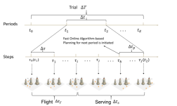
Figure 3: Three-level trial-period-step time hierarchy for ABS movement optimization.

One trial for problem (P1) is equally divided into $E$ periods, where each period has $J\triangleq I/E$ steps and thus lasts for $\Delta t\triangleq\Delta T/E=J\cdot\Delta\tau$ s, as illustrated in Fig. 3. As a preliminary study, we focus on scenarios characterized by low/moderate GU mobility, and assume that the distribution of GUs between two consecutive periods exhibit only minor variations. Each period consists of two non-overlapping phases, i.e., flight and serving, each with a duration of $\Delta t_{f}$ s and $\Delta t_{s}$ s, respectively, with $\Delta t_{f}+\Delta t_{s}=\Delta t$. For a target period (e.g., $t_{1}\sim t_{2}$ in Fig. 3), a preliminary planning procedure spanning $\Delta t_{p}$ ($\Delta t_{p}\leq\Delta t$) is initiated beforehand, which takes the newly reported GU location information (e.g., at time instant $t_{1}-\Delta t_{p}$) as input, and uses the fast online algorithm to output the candidate ABS placement solutions. Each ABS adjust its moving speed to reach the destination in the flight period and hover until the end of the serving period. Next, we focus on our proposed fast online algorithm.

III-B Fast Online Algorithm

Due to the NP-hard nature of the problem (P1), using traditional open source solver (SCIP) might impose high computational complexity to solve such ABS placement problem as the problem size increases. In [10], the author proposes a fast online algorithm which is used to solve a class of BILP problems rapidly, whereby the obtained solution achieves the close-to-optimal performance. It essentially conducts (one-pass) projected stochastic subgradient descent within the dual space. Here we use the fast online algorithm [10] with tailored modifications to solve our BILP problem. Firstly, we rewrite the constraints (9) $\sim$ (13) into matrix and vector form as

where $\boldsymbol{1}_{U_{n}^{\prime}}\in\mathbb{R}^{(U^{{}^{\prime}})}$ is an elementwise indicator function for the feasible ABS grid index set $U_{n}^{{}^{\prime}}$ of each ABS $n$. Denote $\boldsymbol{E}\in\mathbb{R}^{(1+N+U^{{}^{\prime}}V+V)\times(V+U^{{}^{\prime}})}$ as the coefficient constraint matrix, $\boldsymbol{x}\in\mathbb{R}^{(V+U^{{}^{\prime}})}$ as the variable vector, and $\boldsymbol{l}\in\mathbb{R}^{(1+N+U^{{}^{\prime}}V+V)}$ as the right-hand side constant vector. Note that the superscript $(i)$ is omitted here for simplicity, and we focus on maximizing the number of covered GUs for a given ABS placement subproblem, as given by

$$\text{(P2):}~{}\max{} \sum_{\begin{subarray}{c}v\in V\end{subarray}}C_{v}\triangleq\boldsymbol{r}^{T}\boldsymbol{x}$$

s.t. $$\boldsymbol{E}\boldsymbol{x}\leq\boldsymbol{l},$$

$$x_{k}\in\left\{0,1\right\},k\in(V+U^{{}^{\prime}}),$$

where $\boldsymbol{r}=(1,\ldots,1,0,\ldots,0)\in\mathbb{R}^{(V+U^{{}^{\prime}})}$ denote the coefficient vector of the objective function. The problem (P2) is a BILP problem involving integer variables. We first apply linear relaxation to the above problem (P2), as given by

$$\text{(P3):}~{}\max{} \boldsymbol{r}^{T}\boldsymbol{x}$$

s.t. $$\boldsymbol{E}\boldsymbol{x}\leq\boldsymbol{l},$$

$$\boldsymbol{0}\leq\boldsymbol{x}\leq\boldsymbol{1}.$$

According to [15], the dual linear programming (DLP) problem of (P3) is given by

$$\text{(P4):}~{}\min{} \boldsymbol{l}^{T}\boldsymbol{y}+\boldsymbol{1}^{T}\boldsymbol{s}$$

s.t. $$\boldsymbol{E}^{T}\boldsymbol{y}+\boldsymbol{s}\geq\boldsymbol{r},$$

$$\boldsymbol{y}\geq\boldsymbol{0},\boldsymbol{s}\geq\boldsymbol{0},$$

where dual decision variables are $\boldsymbol{y}\in\mathbb{R}^{(1+N+U^{{}^{\prime}}V+V)}$, $\boldsymbol{s}\in\mathbb{R}^{(V+U^{{}^{\prime}})}$. Denote the optimal solution to (P3) and (P4) as $\boldsymbol{x}^{*}$, $\boldsymbol{y}^{*}$ and $\boldsymbol{s}^{*}$. Based on complementary slackness condition[15], we have

$$x_{k}^{*}=\left\{\begin{array}[]{ll}1,&r_{k}>\boldsymbol{e}_{k}^{T}\boldsymbol{y}^{*};\\ 0,&r_{k}<\boldsymbol{e}_{k}^{T}\boldsymbol{y}^{*},\end{array}\right.$$ (17)

where $\boldsymbol{e}_{k}$ denotes $k$-th column of the matrix $\boldsymbol{E}$. Plug the constraints in (P4) to its objective function to remove the dual decision variables $\boldsymbol{s}$. The reformulated problem is given by

$$~{}\min~{} \boldsymbol{l}^{T}\boldsymbol{y}+\boldsymbol{1}^{T}(\boldsymbol{r}-\boldsymbol{E}^{T}\boldsymbol{y})$$ (18)

s.t. $$\boldsymbol{y}\geq\boldsymbol{0},$$

For more refined algorithm derivation, we divide the matrix operations into certain vector operations and denote $\boldsymbol{l}=(V+U^{{}^{\prime}})\boldsymbol{d}$. Extract the constant coefficient $(V+U^{{}^{\prime}})$, and we obtain an equivalent form of (P4) that only involves decision variable $\boldsymbol{y}$, as given by

$$\min_{\boldsymbol{y}\geq\mathbf{0}}~{} f(\boldsymbol{y})=\boldsymbol{d}^{T}\boldsymbol{y}+\frac{1}{V+U^{{}^{\prime}}}\sum_{k=1}^{V+U^{{}^{\prime}}}\left(r_{k}-\boldsymbol{e}_{k}^{T}\boldsymbol{y}\right)^{+}$$ (19)

where $(\cdot)^{+}$ denotes the positive part function. The transition from $\boldsymbol{y}_{t}$ to $\boldsymbol{y}_{t+1}$ can be viewed as an implementation of the projected stochastic subgradient descent technique for optimizing problem (19). At each iteration $t$, it updates the vector with the latest observation and performs a projection onto the non-negative orthant to maintain dual feasibility. Concretely, the subgradient of the $t$-th term in (19) evaluated at $\boldsymbol{y}_{t}$ is as follows,

$$\left.\partial_{\boldsymbol{y}}\left(\boldsymbol{d}^{T}\boldsymbol{y}+\left(r_{t}-\boldsymbol{e}_{t}^{T}\boldsymbol{y}\right)^{+}\right)\right|_{\boldsymbol{y}=\boldsymbol{y}_{t}}=\boldsymbol{d}-\left.\boldsymbol{e}_{t}\mathbb{I}\left(r_{t}>\boldsymbol{e}_{t}^{T}\boldsymbol{y}\right)\right|_{\boldsymbol{y}=\boldsymbol{y}_{t}}$$

$$=\boldsymbol{d}-\boldsymbol{e}_{t}x_{t},$$ (20)

where $\mathbb{I}(\cdot)$ denotes the indicator function. We denote $\Xi(\mathcal{P})$ as the function to calculate the currently covered GUs, $\vee$ as the elementwise maximum operator, and $\alpha$ as the step size. According to [16], we also apply the duplication factor $K$ to increase the covered GU number. The pseudo code of the fast online algorithm is described in Algorithm 1.

The algorithm create the first loop by applying the duplication factor $K$ (Line 1). Since the number of variable $C_{v}$ is connected to the number of GU $M$, and GU location set is known in advance, we focus on the grid that located GU. The algorithm initializes a random permutation $q$ which is a random variable index array ranging from 0 to $M+U^{{}^{\prime}}-1$, whereby improving the randomness of the algorithm. Each element in array $q$ indicates the variable index (Line 2). Then, from the complementary slackness condition (17), we utilize constraint matrix $\boldsymbol{E}$ and dual decision variables $\boldsymbol{y}$ to find feasible ABS locations in the second loop (Line 3$\sim$4). Due to the implementation of the projected stochastic subgradient descent technique, we update dual decision variable $\boldsymbol{y}$ based on (III-B) (Line 5$\sim$6). Finally, obtain $\mathcal{P}_{\text{tmp}}$ which is the ABS placement location set of current loop based on $\boldsymbol{x}$. After $K$ loops, we find the algorithm-believed best ABS location set $\mathcal{P}^{*}$ (Line 8$\sim$10). The worst time complexity of this algorithm is $\mathcal{O}(K(M+K_{1}K_{2}))$. But for the site-specific environment, the feasible ABS placement range $U^{{}^{\prime}}$ is significantly smaller than the global range $K_{1}K_{2}$, so the time complexity will tend to $\mathcal{O}(K(M+U^{{}^{\prime}}))$. Based on [10], we denote the optimal objective values of the problem P2 and P3, as $Q_{n}^{*}$ and $R_{n}^{*}$, respectively. The objective value obtained by the algorithm output is denoted as $R_{n}$. The quantity of interest is the optimality gap $Q_{n}^{*}-R_{n}$, which has an upper bound $Q_{n}^{*}-R_{n}\leq R_{n}^{*}-R_{n}$. The expected optimality gap is defined as $\mathbb{E}[R_{n}^{*}-R_{n}]$. According to Theorem 1 in [10], the expected optimality gap is $\mathbb{E}[R_{n}^{*}-R_{n}]\leq(1+N+U^{{}^{\prime}}V+V)(\overline{e}+\overline{d})^{2}\sqrt{V+U^{{}^{\prime}}}$, where $\|\boldsymbol{e}_{k}\|_{\infty}\leq\overline{e},k=1,\ldots,V+U^{{}^{\prime}}$, $\|\boldsymbol{d}_{i}\|_{\infty}\leq\overline{d},i=1,\ldots,1+N+U^{{}^{\prime}}V+V$. According to our above optimization of the algorithm, we reduce the optimality gap to $(1+N+U^{{}^{\prime}}V+V)(\overline{e}+\overline{d})^{2}\sqrt{M+U^{{}^{\prime}}}$.

1 Input: GU location set $\mathcal{Q}$, initial ABS location set $\mathcal{P}$, feasible ABS placement index set $U^{{}^{\prime}}$ and duplication factor $K$.

2 Output: Algorithm-believed best ABS location set $\mathcal{P}^{*}$.

1:for $i$ in $K$ do

2: Initialize random permutation $q$.

3: for $t$ in $q$ do

4:  $x_{t}=\left\{\begin{array}[]{ll}1,&r_{t}>\boldsymbol{e}_{t}^{T}\boldsymbol{y}_{t}\\ 0,&r_{t}<\boldsymbol{e}_{t}^{T}\boldsymbol{y}_{t}\end{array}\right.$

5:  $\boldsymbol{y}_{t+1}=\boldsymbol{y}_{t}+\alpha\left(\boldsymbol{e}_{t}x_{t}-\boldsymbol{d}\right)$

6:  $\boldsymbol{y}_{t+1}=\boldsymbol{y}_{t+1}\vee\boldsymbol{0}$

7: end for

8: Obtain $\mathcal{P}_{\text{tmp}}$ based on $\boldsymbol{x}$.

9: if $\Xi$($\mathcal{P}_{\text{tmp}}$) $>$ $\Xi$($\mathcal{P}^{*}$) :

10:  $\mathcal{P}^{*}\leftarrow\mathcal{P}_{\text{tmp}}$

11:end for

Algorithm 1 Fast Online Algorithm for ABS Placement

IV Numerical Results

In this section, we present comprehensive simulation results to demonstrate the effectiveness of our proposed algorithm. Comparisons are made against directly using open sourse solver (SCIP)[11] and one of the state-of-the-art DRL methods (TD3)[12]. The setting of hyperparameters is consistent with the [12]. In addition, we introduce the K-means initiated evolutionary algorithm (NM) which initially employs the K-means algorithm to generate initial ABS locations, and then utilizes the EA-based mutation strategy within the specified mutation range to generate mutated ABS sets during the planning period. Each mutation set is subject to the constraints (1) and (2). In $K_{m}$ rounds of mutation, we select the ABS set with the highest CR as the next optimal positions. The performance metric includes the ACR, average planning time ($\overline{t}$) of the entire trial, and the CR of each step. The default parameters are listed in the following if not stated otherwise: $D_{1}=1000$ m, $D_{2}=1000$ m, $K_{1}=K_{1}^{{}^{\prime}}=40$, $K_{2}=K_{2}^{{}^{\prime}}=40$, $h_{w}[l]\sim\textrm{Uniform}(30,89)$ m, $L=300$, $H=90$ m, $h_{q}=1$ m, $V^{\max}_{p}=30$ m/s, $V_{q}=2$ m/s, $K=3$, $K_{m}=3000$, $\Delta T=200$ s, $\Delta t=20$ s, $\Delta t_{f}=10$ s, $\Delta t_{s}=10$ s, $\Delta t_{p}=5$ s, $\Delta\tau=1$ s, $P=5$ dBm, $\sigma^{2}=-112$ dBm, $\bar{\gamma}=3$ dB, $\eta=3$ dB.

IV-A ABS Trajectory Visualization

In this section, we select several consecutive steps to visualize the flight trajectory and coverage status of the ABSs. The initial locations and flight trajectory are shown in Fig. 4. For the considered example, the coverage rate is improved from 0.8 to 0.95 by utilizing our proposed algorithm.

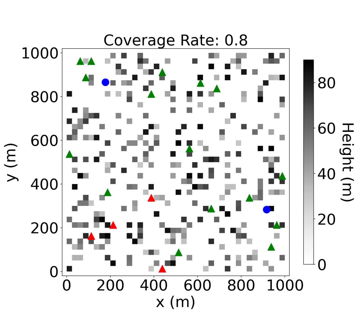
(a) initial locations

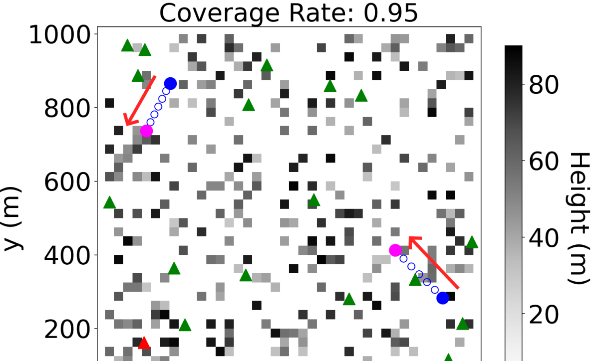
(b) flight trajectory

Figure 4: ABS flight trajectory during consecutive steps ($N=2$, $M=20$). The squares represent the generated BBs, whose color darkness indicates their heights. The initial ABSs is denoted by blue points, and the final ABSs is denoted by magenta points. The hollow points represent the positions of ABSs during the flight period. Triangles symbolize GUs, with green and red coloring indicating covered and uncovered GUs, respectively.

IV-B Grid Length Sensitivity and Quantization Error

In this section, we change the grid length to analyze the quantization error of the approximation in Section II-D. In the simplified situation, we use the grid center $\boldsymbol{b}_{v}$ to represent any given GU located in the grid $v$, while in actual situation, we use the real locations of any given GU. The results of different grid lengths and quantization errors are shown in Table I.

It can be seen from the Table I that the approximation produces a certain quantization error while simplifying the problem, but when the grid length decreases, the quantization error between the simplified situation and the actual situation shows a gradually decreasing trend. Moreover, due to the decrease of grid length, more grids can be chosen for the ABS placement, thus improving the average coverage rate. Therefore, there exists a general trade-off between the CR performance, quantization error and the algorithm complexity, whereby the grid length in a given area needs to be chosen carefully depending on the application requirements.

TABLE I: Grid length sensitivity and quantization error ($N=5$, $M=100$, $trials=20$).

Grid Length(m)	12.5	25	50
Simplified Situation(ACR)	0.942	0.917	0.891
Actual Situation(ACR)	0.929	0.891	0.855
Quantization Error	0.013	0.026	0.036

IV-C Dynamic Case With Moving GUs

In this section, we consider two dynamic scenarios with moving GUs and evaluate the average performance (ACR, $\overline{t}$) by averaging over 5 different trials, each with 400 steps. Note that TD3 fails to converge in larger problems. The results are shown in Table II, Fig. 5 and Fig. 6.

Our algorithms exhibit superior performance compared to the TD3 and NM methods in terms of average CR in both two dynamic cases, meanwhile, our algorithm significantly reduces average planning time compared to using SCIP directly, due to the implementation of the fast online approach that swiftly produces ABS location set. Due to the real-time constraints in our problem, it is worth noting that the results obtained by SCIP only serve as a loose upper bound, which is difficult, if not impossible, to achieve in practice.

IV-D Accommodation To Complex/Dynamic Scenarios

In large scale scenarios, we also compare the algorithms under different site-specific environments (e.g., with the number of BBs from 200 to 400 in the considered area). The ACR performance of the SCIP, Ours, NM are shown in Fig. 7. It can be seen that, in general, the ACR of the three algorithms decreases as the number of BBs increases. Notably, our proposed algorithm consistently outperforms the NM method, and the disparity between ours and SCIP remains relatively stable even as the building size increases. In addition, we also change GU speeds (2$\sim$10 m/s) to observe ACR performance of different algorithms. It is observed that our proposed algorithm still achieves a high ACR under moderate GU speeds, and consistently outperforms NM methods.The detailed results are omitted for brevity.

TABLE II: The average performance in two scenarios

Algorithms	SCIP	Ours	TD3	NM
ACR($N=2$, $M=20$)	0.90	0.84	0.79	0.64
$\overline{t}$(s)($N=2$, $M=20$)	1.47	0.92	0.96	1.18
ACR($N=5$, $M=100$)	0.95	0.91	$-$	0.78
$\overline{t}$(s)($N=5$, $M=100$)	5.56	1.79	$-$	1.87

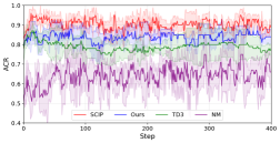
Figure 5: Step-wise CR performance of the four different algorithms with $400$ steps over 5 different trials($N=2$, $M=20$).

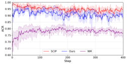
Figure 6: Step-wise CR performance of the three different algorithms with $400$ steps over 5 different trials($N=5$, $M=100$).

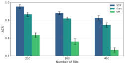
Figure 7: ACR performance with different number of BBs ($N=5$, $M=100$). The height of bars represents the average value of ACR, while the black error bars indicate the standard deviations.

V Conclusion

This paper investigates the movement optimization of multiple ABSs to maximize the average coverage rate of mobile GUs in a site-specific environment. The problem is NP-hard in general and further complicated by the complex propagation environment and GU mobility. To tackle this challenging problem, we construct GCM and formulate the problem into a BILP problem. We introduce a fast online algorithm which can solve such problem rapidly and efficiently. Optimality bounds are also provided for the proposed algorithm. Numerical results demonstrate that our proposed algorithm achieves a high CR performance close to that obtained by the open source solver (SCIP), yet with significantly reduced running time. In addition, the algorithm also notably outperforms the K-means initiated evolutionary algorithm and TD3 in terms of CR performance and/or time efficiency.

References

- [1] Y. Zeng, Q. Wu, and R. Zhang, “Accessing from the sky: A tutorial on UAV communications for 5G and beyond,” Proc. IEEE, vol. 107, no. 12, pp. 2327–2375, Dec. 2019.
- [2] J. Lyu, Y. Zeng, R. Zhang, and T. J. Lim, “Placement optimization of UAV-mounted mobile base stations,” IEEE Commun. Lett., vol. 21, no. 3, pp. 604–607, Mar. 2017.
- [3] B. Galkin, J. Kibilda, and L. A. DaSilva, “Deployment of UAV-mounted access points according to spatial user locations in two-tier cellular networks,” in Wireless Days, Mar. 2016, pp. 1–6.
- [4] Z. Wang, L. Duan, and R. Zhang, “Adaptive deployment for UAV-aided communication networks,” IEEE Trans. Wireless Commun., vol. 18, no. 9, pp. 4531–4543, Sep. 2019.
- [5] A. Al-Hourani, S. Kandeepan, and S. Lardner, “Optimal LAP altitude for maximum coverage,” IEEE Wireless Commun. Lett., vol. 3, no. 6, pp. 569–572, Dec. 2014.
- [6] S. Bi, J. Lyu, Z. Ding, and R. Zhang, “Engineering radio maps for wireless resource management,” IEEE Wireless Commun., vol. 26, no. 2, pp. 133–141, Apr. 2019.
- [7] J. Qiu, J. Lyu, and L. Fu, “Placement optimization of aerial base stations with deep reinforcement learning,” in Proc. IEEE Int. Conf. Commun. (ICC), June 2020, pp. 1–6.
- [8] P. Zhen, B. Zhang, C. Xie, and D. Guo, “A radio environment map updating mechanism based on an attention mechanism and siamese neural networks,” Sensors, vol. 22, no. 18, p. 6797, 2022.
- [9] R. Levie, Ç. Yapar, G. Kutyniok, and G. Caire, “Radiounet: Fast radio map estimation with convolutional neural networks,” IEEE Trans. Wireless Commun., vol. 20, no. 6, pp. 4001–4015, 2021.
- [10] X. Li, C. Sun, and Y. Ye, “Simple and fast algorithm for binary integer and online linear programming,” Advances in Neural Information Processing Systems, vol. 33, pp. 9412–9421, 2020.
- [11] K. Bestuzheva, M. Besançon, W.-K. Chen et al., “The SCIP Optimization Suite 8.0,” Zuse Institute Berlin, ZIB-Report 21-41, December 2021.
- [12] J. Lyu, X. Chen, J. Zhang, and L. Fu, “Spatial deep learning for site-specific movement optimization of aerial base stations,” IEEE Trans. Wireless Commun., pp. 1–1, December 2023.
- [13] H. Xie, D. Yang, L. Xiao, and J. Lyu, “Connectivity-aware 3D UAV path design with deep reinforcement learning,” IEEE Trans. Veh. Technol., vol. 70, no. 12, pp. 13 022–13 034, 2021.
- [14] 3GPP-TR-36.777, “Enhanced LTE support for aerial vehicles,” 3GPP Technical Report, Dec. 2017.
- [15] D. G. Luenberger, Y. Ye et al., Linear and nonlinear programming. Springer, 1984.
- [16] W. Gao, D. Ge, C. Sun, and Y. Ye, “Solving linear programs with fast online learning algorithms,” in Proc. Int. Conf. Machine Learning(ICML), 2023.