Isopignistic Canonical Decomposition via Belief Evolution Network
Abstract
Developing a general information processing model in uncertain environments is fundamental for the advancement of explainable artificial intelligence. Dempster-Shafer theory of evidence is a well-known and effective reasoning method for representing epistemic uncertainty, which is closely related to subjective probability theory and possibility theory. Although they can be transformed to each other under some particular belief structures, there remains a lack of a clear and interpretable transformation process, as well as a unified approach for information processing. In this paper, we aim to address these issues from the perspectives of isopignistic belief functions and the hyper-cautious transferable belief model. Firstly, we propose an isopignistic transformation based on the belief evolution network. This transformation allows for the adjustment of the information granule while retaining the potential decision outcome. The isopignistic transformation is integrated with a hyper-cautious transferable belief model to establish a new canonical decomposition. This decomposition offers a reverse path between the possibility distribution and its isopignistic mass functions. The result of the canonical decomposition, called isopignistic function, is an identical information content distribution to reflect the propensity and relative commitment degree of the BPA. Furthermore, this paper introduces a method to reconstruct the basic belief assignment by adjusting the isopignistic function. It explores the advantages of this approach in modeling and handling uncertainty within the hyper-cautious transferable belief model. More general, this paper establishes a theoretical basis for building general models of artificial intelligence based on probability theory, Dempster-Shafer theory, and possibility theory.
keywords:
Dempster-Shafer theory, canonical decomposition, isopignistic transformation, belief evolution network, hyper-cautious transferable belief model , uncertainty measure , information fusion[inst1]organization=Institute of Fundamental and Frontier Science, organization=University of Electronic Science and Technology of China,city=Chengdu, postcode=250014, country=China
[inst5]organization=School of Medicine, organization=Vanderbilt University, city=Nashville, postcode=37240, country=USA
1 Introduction
Dempster-Shafer (DS) theory of evidence, also known as belief function theory, is an effective artificial intelligence tool for modeling and handling uncertainty in partial knowledge environments. First, the DS theory is derived from probability multi-valued mapping [6] and is formalized as a random coding semantics [32]. By assigning the mass to the frame’s power set, the basic probability assignment (BPA) generalizes the probability distribution. Non-refinable beliefs are assigned on the multi-element propositions. Upon receiving enough knowledge, these beliefs can be transferred into singletons, and the BPA equals a probability distribution. Hence, the BPA can be viewed as a probability distribution that introduces ignorance through the multi-valued mapping. DS theory also has connections with other useful uncertainty theories, such as possibility theory [57], imprecise probability theory [3], rough set theory [4], lattice theory [52], etc, which makes exploring the information distribution on the belief structure a critical part of modeling uncertainty. Dempster’s rule of combination (DRC) is proposed for fusing BPAs from multiple independent and credible sources, which is capable of updating information without prior knowledge. Based on the advantages of modeling and handling uncertainty, DS theory is widely applied in conflict analysis [26], evidential reasoning [39], fault diagnosis [44], expert decision making [40, 42] and machine learning under uncertain environments [51, 27, 22]. In addition, novel interpretations and extensions of belief structures are proposed for representing uncertainties of higher types and orders. In terms of interpretation, Smets and Kennes [36] propose a transferable belief model (TBM) that utilizes two levels to quantify and handle the agent’s beliefs. Yang and Xu [50] introduce weights and reliability into DRC to propose the ER rule for handling unimportant and unreliable granules. Pichon et al. [31] model the meta-knowledge on belief structure, which provides a general representation framework for contextual knowledge. In terms of the extension, the relations among elements are discussed in D number theory [7] and Dezert-Smarandache Theory [14]. The complex-valued mass is used to predict the interference effect [41, 29] and its phase is considered as a certainty degree [28]. Deng [9] introduces the order into multi-element propositions and proposes the random permutation set theory, which can be viewed as a layer-2 belief structure [54].
In recent years, belief structure-based information processing methods have flourished. However, due to the complexity of the belief structure, it is difficult for BPA to represent the supporting to an element and its construction logic. The identical information content transformation provides multiple views to reflect the uncertainty of BPA, where identical information content means reversible transformation. The most popular transformations are the belief function and plausibility function (Eq. (1)), which show the proposition’s lower and upper degree of support. Based on the inclusion relationship between propositions, the function 111For the normalized mass function, function equals belief function and commonality function (Eq. (2)) are defined, which allows for a more simple calculation of the conjunctive combination rule and disjunctive combination rule [10]. These transformations are defined based on the set relation between propositions, and their transformed functions are used to reflect beliefs about the propositions. In addition, canonical decomposition is another way to realize the identical information content transformation. Compared to set relation-based functions, canonical decomposition emphasizes generating the elementary components of BPA and providing an interpretable construction process. Smets [33] proposes a canonical decomposition for non-dogmatic mass functions, whose results are denoted as the weights of the belief function. For an -element frame, a non-dogmatic mass function can be decomposed as simple mass functions’ fusion and retraction via CCR. Denœux [10] proposes the dual form of the diffidence function, called function, and develops them into the cautious combination rule (CauCR) and bold combination rule (BCR), respectively. However, Smets’ canonical decomposition only aims at non-dogmatic function, and its semantics lack distinct theoretical support. Pichon [30] proposes the -canonical decomposition based on the Teugels’ representation of the multivariate Bernoulli distribution. Its result function can be written as dependent fusions of simple mass functions, where the dependent coefficient is the covariance in Teugels’ representation. Pichon’s canonical decomposition covers all belief functions and has distinct semantics in multivariate Bernoulli distribution. Under the belief function frame, however, the semantics of positive and negative and the range of are unclear, so how to capture function from data and knowledge needs further exploration.
Isopignistic transformation is also an identical information content transformation, but have not previously been discussed. It is derived from the isopignistic domain, which means a set of belief functions whose pignistic probability transformation (PPT) results are the same [20]. Therefore, isopignistic transformation means transferring beliefs in the isopignistic domain. Inspired by the fractal theory, Zhou and Deng [55] simulate the process of PPT via the fractal-based belief (FB) transformation. Though the FB transformation is isopignistic, it cannot realize arbitrary belief functions in the isopignistic domain. In addition, the possibility distribution can be uniquely transformed into a consonant mass function [17]. Since the consonant mass function is BPA with the least commitment degree in its corresponding isopignistic domain, the possibilistic information processing can be seen as the hyper-cautious TBM [34]. PPT also can be realized on the belief evolution network (BEN) [58]. When compared to the FB transformation, BEN hierarchies are based on the cardinality of propositions and only allow beliefs to be transferred between adjacent layers. Hence, the BEN provides a more general frame than FB transformation for isopignistic transformation.
In this paper, we propose an isopignistic belief evolution rule via the BEN, which can realize the isopignistic transformation among all belief functions within its corresponding isopignistic domain. Under the isopignistic canonical decomposition, a belief function can be decomposed as two components. Propensity is the first component, which is a possibility distribution and consists of a hyper-cautious TBM, and commitment is the second component, which is used to adjust the commitment degree from consonant mass function to the input BPA. Our study not only examines the difference between the proposed method and previous canonical decompositions, but also examines the uncertainty composition of the belief function from an isopignistic perspective. Generally, the isopignistic transformation will guide the development of the hyper-cautious TBM, which provides an interface for handling evidential information on possibilistic structures. The contributions of the paper can be summarized as follows: First, we propose an identical information transformation method that can cover the isopignistic domain. Second, based on the proposed transformation, isopignistic canonical decomposition is proposed, which provides a new perspective to interpret the belief function. Finally, we illustrate its significance in specificity measures and information fusion based on the proposed canonical decomposition.
Section 2 introduces some necessary prior concepts. In Section 3, isopignistic transformation is proposed based on the belief evolution network, and in Section 4, the isopignistic canonical decomposition is proposed, which provides a novel interpretable construction process of belief function. Section 5 utilizes the isopignistic function to model and handle uncertainty in hyper-cautious TBM and Section 6 summarizes the entire paper and discusses the further research direction.
2 Basic concepts on Dempster-Shafer theory
Due to the variety of interpretations and notations of DS theory, we will reorganize its basic concepts in this part in order to avoid ambiguity.
2.1 Information representation
Suppose an uncertain variable , its value is taken in an exhaustible closed set, called frame of discernment, . A restriction , called basic probability assignment (BPA) [32] is a mass function to represent the available knowledge about . The mass on the proposition should satisfy and . is called a focal set when , where denotes the decimal representation of Boolean algebraic binary codes [56]. For example, means the proposition , and means the unrefineable beliefs on . Thus, the information distribution under the belief structure corresponding to the -element frame can be represented by a -dimensional vector. The order is determined by the binary corresponding to the subset. The set of focal sets is written as . For the convenient representation, there are some special mass functions:
-
1.
is a normalized mass function when , which equals a credal set mathematically.
-
2.
is a vacuous mass function when , which denotes the total ignorance to and is written as .
-
3.
is a empty mass function when , which denotes the total conflicts and is written as .
-
4.
is a Bayesian mass function when the focal sets are singletons, which equals a probability distribution mathematically.
-
5.
is a simple mass function when there are only two focal sets and one of them is , which can be written as .
-
6.
is a non-dogmatic mass function when .
-
7.
is a consonant mass function when the focal sets are nested, i.e., it satisfies or .
Since the focal sets are elements of the power set, there are some other representations calculated from the set relations, which provide multiple perspectives to model uncertainty. The belief () function and plausibility () function, the two most popular measures, are defined as
| (1) | ||||
where is the complement operation. represents the beliefs of total supporting , and represents the beliefs of total supporting , i.e. the beliefs of non-negating . The belief interval can reflect the degree of imprecision in the restriction to the proposition . As the dual of function 222, commonality (Q) function is defined as
| (2) |
where is the function of the , which satisfies . represents the sum of beliefs of focal sets which contain . , , and functions are identical information content representation, and they can be seen as observing mass function under different coordinate systems.
2.2 Information fusion
Information granules with different states should be fused using different combination rules. Hence, the combination rules are introduced based on the different sources’ states. When there are two mass functions and from distinct and credible sources to describe the restriction of , the conjunctive combination rule (CCR) is the appropriate method to fuse them to describe being more specific, which is denoted as [6, 36]
| (3) |
If executing the normalization after CCR, it is Dempster’s rule of combination (DRC)
| (4) |
Suppose and are the functions of and (Eq. 2), then CCR has a simpler form
| (5) |
Hence, CCR can be attained by multiplying the focal sets with their respective counterparts within the representation of the function, a simpler approach compared to mass functions. In addition, its de-combination rule also can be realized via function
| (6) |
When there are two mass functions and originating from different sources, and if at least one is credible, then the disjunctive combination rule (DCR) is the appropriate method to combine them to describe , which is denoted as
| (7) |
Since function is dual with function (Eq. 2), DCR and its de-combination rule can be realized by function
| (8) |
| (9) |
2.3 Canonical decompositions
Canonical decomposition is the transformation of a mass function into an elementary components that uniquely points to the original mass function. Similarly, it can be understood as a transformation of the identical information content, but it focuses on interpreting the construction process of the belief functions. For a non-dogmatic mass function under an -element frame, its diffidence function 333It is also called weights of belief function. is denoted as [33, 15]
| (10) |
where represents positive integer. When , it can be written as a simple mass function ; when , it can be written as a simple mass function . The mass function satisfies
| (11) |
Hence, we can decompose any non-dogmatic mass function into simple mass functions’ fusions and retractions 444It is defined in [15], which equals de-combining a simple mass function. Since the function is the dual form of function. The dual diffidence function also can be extended as [10]
| (12) |
and the arbitrary unnormalized mass function can be written as
| (13) |
On the representations of the diffidence function and function, the cautious combination rule (CauCR) and bold combination rule are defined as [10]
| (14) | ||||
In addition to methods based on independent information fusion, -canonical decomposition interprets from the dependent fusion perspective. For any mass function under an -element frame, the function is denoted as [30]
| (15) |
where is column vector form of . In the information fusion framework proposed by Pichon [31], elements correspond to the reliability of sources. When , , it means that the reliability of these sources is independent of each other, and can be written as . As for the other cases, quantifies the covariance of the reliability of the sources represented by the elements in .
The purpose of this section is to demonstrate the common methods for representing and processing information in DS theory, which are necessary for understanding this paper.
3 Isopignistic transformation via belief evolution network
3.1 Problem description
When there is no knowledge available to influence an agent’s belief, the beliefs should be transferred into singletons for decision making. On the basis of the linearity principle, Smets [35] derives the pignistic probability transformation (PPT), which is denoted as
| (16) |
and its normalized version is
| (17) |
Due to the irreversible nature of data dimensionality reduction, there exists an infinite number of belief functions with the same .
Definition 3.1.1 (Isopignistic domain & transformation)
For a probability distribution , its isopignistic domain contains all BPAs whose s equal , which is defined as
| (18) |
If a reversible transformation of belief functions, denoted as , satisfies , it is an isopignistic transformation. Hence, the input and output of the isopignistic transformation belong to the same isopignistic domain.
The isopignistic transformation does not influence the preference of decision making, but only adjusts the commitment degree of the BPA. It aims to find a general transformation method that can connect all mass functions in an isopignistic domain.
3.2 Belief evolution network
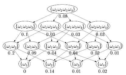
[58] introduces causality into the hierarchical hypothesis space and proposes the belief evolution network (BEN). BEN can be seen as a constrained beliefs transferring method. Beliefs can only be transferred between focal sets that are adjacent in cardinalities, and only one layer can be transferred at a time. The structure of the BEN under an -element frame is shown in Figure 1.

Definition 3.2.1 (belief evolution network)
An -element frame can be represented as a directed acyclic graph , where , . For the node which satisfies , it has a distribution represents the proportion of transferred beliefs. For the edge , it has a distribution represent the proportion of ’s transferred beliefs, which satisfies . The is called the belief evolution network (BEN). Algorithm 1 shows the specific process of executing BEN on , which can be written as .
It is obvious that , , executing BEN on can be seen as a probability transformation. Dezert et al. [12] propose a hierarchical probability transformation via transferring belief between adjunct layers. Based on the BEN, Zhou et al. [58] independently present a similar result, but use a different coefficient to constrain the transferring belief ratio. In addition, choosing appropriate , BEN can cover the most of probability transformations.
Proposition 3.2.1
If a probability transformation method satisfies upper and lower bounds consistency [21], i.e. , it also can be realized on the BEN.
Proof 3.2.1
If the range of and is , after executing BEN, the masses of singletons should satisfy . In BEN, the receiving beliefs focal sets must be the subset of the transferring beliefs focal sets. Hence, for the , its potential transferred beliefs should satisfy . Hence, BEN can cover all probability distributions which satisfy the .\qed
Proposition 3.2.2
If the BEN adheres to the condition and with , ensuring that , then the resultant evolution of any BPA will coincide with its .
Proof 3.2.2
For a mass in , its contribution for of all elements in can be written as . After executing BEN in the ’s corresponding layer, the mass are divided as pieces to , where . So the contributions of to is . Based on the Eq. (16), the contributions of for its is . Though the number of receiving the beliefs from is , for an element , it only exists in focal sets after evolution. The ’s contribution for its remains . Hence, when the , the BEN equals the PPT.\qed
This part delineates the definition of BEN from the perspective of a directed acyclic graph and delves into the probability transformation through BEN. Given BEN’s operation on mass within a hierarchical structure, it introduces two coefficient distributions, denoted as and , serving to articulate and represent uncertainty.
3.3 Isopignistic transformation
Building upon Proposition 3.2.2, one may conceptualize PPT as a distinctive instance of BEN, wherein BEN’s takes the form of a uniform distribution and takes . When adjusting the values of within the range of , while maintaining uniform distributions for , executing BEN on can be seen as an isopignistic transformation. Since edges in BEN direct from propositions with larger cardinalities to those with smaller cardinalities, and considering that is a positive value, the only can be derived towards heightened commitment and reduced ignorance. In order to cover the isopignistic domain, backward transferring is necessary. Thus, the isopignistic transformation can be performed by executing twice BEN, where the first step is forward and the second step is backward.
Definition 3.3.1 (Isopignistic transformation)
Consider BPAs and under the frame , coexisting within an isopignisitc domain. The transformation is called the isopignisitc transformation. has forms and , where represents the transferred beliefs and represents its proportion. Under an isopignistic transformation, they are forms representations with identical information content. The generations of and are shown in Algorithm 2, and the transformation from to via or is shown in Algorithm 3.
In Algorithm 3, it is obvious that the and are equal. The transfer process via is where is equal to . Thus, as long as either or is known, the transformation can be executed, and the other distribution can be derived. There are the following differences between the isopignistic transformation and the BEN in Definition 3.2.1. Firstly, as the isopignistic transformation preserves consistency, according to Proposition 3.2.2, for the node , it must satisfy . Therefore, in the isopignistic transformation, the BEN does not need to consider the coefficient . Secondly, backward transfer is introduced to achieve the reduced commitment transformation, so the range of values of is extended to . In order to illustrate the specific transfer process, Example 3.3.1 is used to execute Algorithms 2 and 3 respectively.
Example 3.3.1
-
1.
In terms of the forward transfers and the loop with ,
Based on the Line 10,
-
2.
In terms of the forward transfers and the loop with ,
Based on the Line 10,
-
3.
In terms of the forward transfers and the loop with ,
-
4.
Since has transformed to , the and can be output as
-
1.
In terms of the forward transfers and the loop with ,
When ,
-
2.
In terms of the backward transfers, and the loop with ,
The above numerical example demonstrates that and are equivalent in the isopignistic transformation, but they play distinct roles for further information processing.
Proposition 3.3.1 (role of )
In the context of an isopignistic transformation where , its inverse transformation is denoted as and it satisfies .
Proof 3.3.1
For the focal set , the evolution process is and when and . When , it means transferring from the to s, and when , it means receiving from s. Hence, negating the can realize the inverse transformation.\qed
Proposition 3.3.2 (role of )
If all values of lie within the range , for any arbitrary BPA , the outcome of the transformation using remains a BPA. In other words, it adheres to the conditions and .
Proof 3.3.2
In terms of the forward transfer, it should satisfy , and the corresponding evolution is
and
when and . Since the , satisfies that and locating in the and
In terms of the backward transfer, it should satisfy , and the corresponding evolution is
and
when and . Since the , satisfies that for . In addition
and the number of is , so satisfies .\qed
Proposition 3.3.3 (transmittability)
Given two isopignistic transformations, and , they satisfy and . The transformation from to can be written as , where .
Proof 3.3.3
In terms of the focal set , for the transformation from to , it satisfies , and for the transformation from to , it satisfies . The above equations can derive that , which is same with that transforming into via . In terms of the focal sets s, which satisfy and , for the transformation from to , they satisfy , and it has similar result in and , . Through the same derivation has . Hence, the isopignistic transformation satisfies transmittability. \qed
Proposition 3.3.4 (ergodicity)
Given an and its associated isopignistic domain , the existence of a suitable allows the transformation of into any arbitrary .
Proof 3.3.4
Since the original and the target are in the identical isopignistic domain, they have equal s. According to the Proposition 3.2.2, they can be transformed to through , and . Based on the Proposition 3.3.1, the transformation from to can be realized via . Based on the Proposition 3.3.3, the path from to is . Hence, the proposed transformation can cover the whole isopignistic domain.\qed
3.4 Discussion
In this section, we introduce an isopignistic transformation method via BEN. This method facilitates the establishment of a transformation pathway between a given BPA and any other BPA within its corresponding isopignistic domain. We introduce two coefficient distributions, and , to determine the transformation process. signifies the specific beliefs associated with each transfer, while denotes the proportion of each transfer. These distributions can be reciprocally represented under the same pair of BPAs. Notably, is particularly suited for executing inverse transformations (Proposition 3.3.1) and merging of multiple transformations (Proposition 3.3.3). On the other hand, excels in providing a suitable range, ensuring that any value within this range can generate a valid BPA (Proposition 3.3.2).
4 Isopignistic canonical decomposition
4.1 Motivation
4.1.1 From the canonical decomposition perspective
Canonical decomposition stands out as a pivotal research topic in the DS theory. It not only offers a novel evidential information representation but also furnishes an interpretable construction process for BPAs, thereby reinforcing the connection between data, knowledge, and BPAs. Among the previous approaches, there are two main perspectives proposed by Smets [33] and Pichon [30]. Moreover, certain optimization-based decomposition methods [13, 43] are omitted from this paper owing to their limited interpretability, and the outcomes of such decompositions do not yield elementary pieces. In terms of Smets’ canonical decomposition, it can transform the non-dogmatic BPA into the conjunctive junction of simple mass functions (Eq. (10)). Smets employs the support and doubt to elucidate its semantics. In the TBM, a simple mass function also can be perceived as an unreliable testimony [36], a non-dogmatic mass function can thus be conceptualized as a composition of supporting and doubtful testimonies. However, it is important to note that the non-dogmatic mass function falls short of representing the complete spectrum of BPAs, even though it can approximate the propensity of any BPA. This limitation is deemed mathematically unsatisfactory. The diffidence function representing doubt entails intricate restrictions on the range of its values [15], making it challenging to establish connections with external knowledge and data. Consequently, while Smets’ canonical decomposition elucidates the construction process of mass functions, its practical BPA generation is hindered. In addition, Pichon notes that Smets’ canonical decomposition lacks rigorous mathematical theoretical support, and criticizes its interpretation of doubtful beliefs as being inappropriate. Hence, -canonical decomposition [30] is proposed to resolve the above problems, which is induced from the Teugels’ representation of the multivariate Bernoulli distribution (Eq. (15)). The -canonical decomposition is interpreted as dependent information fusion among sources, wherein the dependent coefficient aligns with the covariance in Teugels’ representation. In addition, function is effective for all belief functions. However, similar to Smets’ method, the range of values for the function remains unclear, and its interpretation within the belief function framework is ambiguous. For instance, when , it signifies that the elements in are independent. When or , their meanings from the perspective of fusion under the dependent sources lacks distinct interpretations, which constrains the connections with data and knowledge. Hence, the quest for a canonical decomposition capable of addressing the aforementioned concerns remains a significant open issue.
4.1.2 From the hyper-cautious TBM perspective
DS theory and possibility theory [18, 37] both serve as effective tools for representing incomplete and imprecise information. The relationship between them and their consistency in handling uncertainty have been subjects of discussion for many years [57]. A possibility distribution can be uniquely transformed into a consonant mass function , and its function aligns consistently with the possibilities of the corresponding focal sets [17]. Dubois et al. [20] have demonstrated that the consonant mass function exhibits the least commitment degree within its isopignistic domain. Considering the principle of the least commitment, Smets suggests that possibility theory can be viewed as a hyper-cautious TBM [34], which provides a perspective for fusing evidential information on the possibilistic structure. However, consonant mass function, possibility distribution, and probability distribution are -dimensional distributions. Transforming the standard BPA to any of them entails a mathematically irreversible reduction in dimensionality. If the links between a possibility distribution and its isopignistic BPAs are not established, the reversibility of the credal level in a hyper-cautious TBM remains unattainable. In this paper, we propose a canonical decomposition from the hyper-cautious TBM perspective, which provides a novel perspective for interpretable BPA construction.
4.2 Isopignistic canonical decomposition
The principle of least commitment is a crucial guiding principle for modeling information within the belief structure. It stipulates that, for uncommitted testimonies, the information distribution should be represented in its least committed form [34]. In [20], a measure for non-commitment degree is denoted as
| (19) |
and it proves that the consonant BPA has the highest non-commitment degree in its isopignistic domain, i.e., , . Since a consonant mass function can be transformed to a possibility distribution uniquely via
| (20) |
where function is the contour function, which equals singletons of function. Given a possibility distribution , it can also be transformed into a consonant BPA. Let denote the th largest possibility in , and rewrite it as . The consonant BPA is [17]
| (21) |
where . Hence, by combining the possibility distribution with the isopignistic transformation, we introduce the concept of isopignistic canonical decomposition.
Definition 4.2.1 (isopignistic canonical decomposition)
Given a BPA defined under an -element frame, it can be transformed into an isopignistic () function on the belief structure. is equivalent to , and they convey the same meaning. represents the possibility of under the least committed case of the isopignistic domain. For with , takes two forms: and . These forms align consistently with the and functions in isopignistic transformations. The generation method of isopignistic function is denoted as , , which is shown in Algorithm 4. The inverse transformation from isopignistic function to BPA is denoted as , , which is shown in Algorithm 5.
Since the isopignistic function is calculated from the isopignistic transformation, and represent transferred beliefs from different perspectives, and they possess identical information contents. Example 4.2.1 shows the specific decompose process via a numerical example.
Example 4.2.1
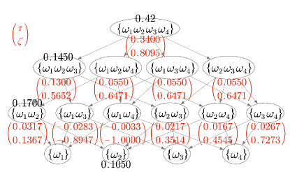
For a BPA under a -element frame , Figure 2 depicts its masses on the structure of the BEN.
Based on the Algorithm 4 the is , and its corresponding possibility distribution is . Additionally, . The corresponding consonant mass function and the remaining isopignistic functions are shown in Fig. 3.
The proposed method decomposes the BPA into two components: propensity and commitment. The propensity component is composed through the singletons of function, whose meaning is same with the element propensity in [53]. For an element, a larger propensity signifies a higher possibility that it is the value of . The commitment component is composed through the multi-element subsets of function. For a focal set with multiple elements, reflects the degree of commitment for negating the elements in . If
and , the will be evolved as
When is a positive value, a higher value implies assigning more beliefs to the negations of its elements. Conversely, when is a negative value, it indicates a decrease in commitment for their negations.
4.3 Properties of the Isopignistic canonical decomposition
To illustrate the advantages of the proposed method, we will analyze its properties from multiple perspectives and present a novel interpretable BPA construction process.
Proposition 4.3.1 (lower and upper bounds)
For a BPA , if its isopignistic function satisfies for , it indicates that the beliefs of concentrate on singletons and the empty set, representing the scenario with the highest degree of commitment. Conversely, if its isopignistic function satisfies for , it characterizes a consonant mass function, signifying the case with the least degree of commitment.
Proof 4.3.1
If the beliefs of concentrate on singletons and the empty set, according to Algorithm 4, , and . In contrast, if is consonant, there is at most one focal set under each cardinality. Given that , after the transfer, . This leads to , and . Hence, the upper and lower bounds for commitment degree in an isopignistic domain is and for , respectively. \qed
From the perspective of Proposition 4.3.1, isopignistic canonical decomposition unveils a path from possibility to probability by constraining the degree of commitment. For any BPA, it should encompass a possibility distribution, representing the lower bound of the degree of commitment, and a probability distribution, signifying the upper bound of the degree of commitment.
Proposition 4.3.2 (reversible construction)
Given a possibility distribution and its corresponding consonant mass function , from the perspective of , selecting any value within the range of ensures that the inverse canonical decomposition result is a BPA. In other words, and .
Proof 4.3.2
The aforementioned isopignistic canonical decomposition can be expressed as an isopignistic transformation , where . In accordance with Proposition 3.3.2, the range of is , consequently, the range of for is also .\qed
In terms of Smets’ canonical decomposition (Eq. (10)), when retracting the beliefs which have not been supported, the result will generate negative value. Although Dubois et al. [15] offer a range for the diffidence function to generate a BPA, the method is intricate and will be affected by the original beliefs. Regarding the -canonical decomposition (Eq. (15)), even though the function of multi-element subsets is interpreted as the covariance among its elements, the range of this function remains unclear.
Example 4.3.1
Suppose a BPA , decompose via isopignistic canonical decomposition (Algorithm 4), -canonical decomposition (Eq. (15)), and Smets’ canonical decomposition (Eq. (10)), respectively, their results are
To verify their abilities to reversibly construct BPAs, we can adjust the values of multi-element subsets in the corresponding functions and observe the changes in the resulting BPAs. According to the interpretation of the functions, the range of values adjusted for and is , while the range of values adjusted for is . The variation of ranges of the BPAs are shown in Figure 4.
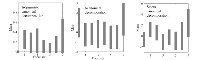
Example 4.3.1 provides a toy numerical experiments to show the advantage of isopignisitc canonical decomposition in reversible BPA construction. The reconstructed BPA varies over the range as we travel through the values of the isopignistic function on the multi-element subsets. The other two methods, however, produce negative beliefs or beliefs greater than one.
Remark 1
The BPA generated from an may not be equal to the obtained from its isopignistic canonical decomposition, but they correspond to the same . To distinguish between these two cases, we denote the former as and leave the latter unchanged, i.e., only the results generated through Algorithm 4 are considered isopignistic functions.
Example 4.3.2 employs a specific instance to illustrate Remark 1 and delineate the distinction between and .
Example 4.3.2
Under a -element frame , given a possibility distribution , and suppose the of other subsets are
The is , the corresponding BPA is
Based on the Algorithm 4, is . Hence, though and generate a same BPA, only is the isopignistic function.
Remark 2
The isopignistic function offers a novel perspective for constructing interpretable BPAs. The singletons of function represent the propensity, aligning with a possibility distribution when the mass function is normalized. The multi-element subsets of function represent the commitment, which adjusts the proportion the ignorant beliefs via isopignistic transformation. Thus, the belief function can be interpreted through isopignistic decomposition as following: the agent’s beliefs about the uncertain variable are quantified as a possibility distribution, which is then adjusted to the BPA through commitment to the distribution. Here commitment to the distribution can be viewed as a form of contextual knowledge, but it has a different meaning with relevance and truthfulness [31].
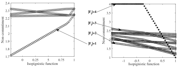
As the quantification of propensity in a minimum commitment case uses the non-commitment measure (Eq. (19)), we utilize its trend with varying isopignistic function to illustrate the points made in Remark 2. Generate a random BPA within a -element framework and calculate its isopignistic function. For singletons , take points uniformly in the interval as the to reconstruct them as BPAs, and calculate their non-commitment degrees. For multi-element subsets, similarly perform the above operations within . Figure 5 shows the variations of non-commitment degree within different s. Varying the in propensity component of BPA does not observe characteristic trends on the non-commitment measure. However, for the commitment component, the non-commitment degree be lower as increases. There is also a significant difference in the range of variation for subsets with different cardinalities. Increasing the transferred beliefs of a subset with a large cardinality will also increase the transferred beliefs of its subsets. Consequently, the subset with the larger cardinality exhibits a greater range of variation.
4.4 Discussion
From the perspective of hyper-cautious TBM and combining with the previously proposed isopignistic transformation we present the isopignistic canonical decomposition in this section. This decomposition is applicable to arbitrary BPAs, allowing them to be decomposed into propensity and commitment components. Propensity signifies the possibility of an element being the target element, and commitment reflects how much ignorance existing in the BPA. The relationship between these two components is recursive; commitment is adjusted only in the context of current propensity, and when the propensity is sufficiently clear, commitment does not require adjustment. When employing as the isopignistic function, modifying the two components separately can lead to operations with entirely distinct implications. Modifying the propensity component alone implies generating BPAs with a relatively equal commitment degree under the new propensity. Adjusting the commitment component alone equals executing an isopignistic transformation. More importantly, compared to the previous methods, the isopignistic function provides a way to generate BPA reversely, i.e. by taking any value within , the generated result must satisfy the mathematical definition of BPA. It is worth noting that the distribution used for the reverse construction BPA is not necessarily equal to the calculated via the constructed BPA. Hence, we specify that only the computed from can be used to generate an isopignistic function.
5 Hyper-cautious transferable belief model
Reviewing the motivation behind proposing the isopignistic canonical decomposition: if we can identify a reversible path from a BPA to its least committed case, it will provide a novel perspective for modeling and handling uncertainty in hyper-cautious TBM. Hence, in this section, in terms of modeling uncertainty, we introduce the methods to measure the specificity from propensity and commitment perspectives respectively. In terms of handling uncertainty, we continue the proposed semantics in [19], and develop the triangular norm-based combination rules via isopignistic function.
5.1 Modeling uncertainty via isopignistic function
How to measure the uncertainty of the BPA is a long discussed topic in DS theory. In terms of the total uncertainty measure, it has been deeply discussed from the discord and non-specificity [25, 23, 38], splitting [8, 55, 5] and granular computing [59] perspectives. In this paper, based on the propensity and commitment components in isopignistic function, we develop the specificity measures of the BPA. Yager [47] analyzes a specificity like measure in DS theory based on the specificity measure of the possibility distribution. Given a BPA under the frame , its specificity measure is defined as
| (22) |
When the is a consonant mass function, and its corresponding possibility distribution is , it will equal the specificity measure of the possibility distribution [45]
| (23) |
where s are the possibilities of elements and is the cardinality of the crisp set . In addition, can be replaced by any other diminishing function as a unified specificity measure of possibility distribution.
Proposition 5.1.1
The specificity measure of a consonant mass function reaches its minimum value in its isopignistic domain.
Proof 5.1.1
The consonant mass function has been proven that reaching the maximum non-commitment case in its isopignistic domain [20]. Based on the Eqs. (19) and (23), the specificity measure and non-commitment measure can be interpreted as a sum of with different suboperations, where the specificity measure is and non-commitment measure is . Since the product of their two suboperations is , when reaches the maximum value in non-commitment measure, it must be reach the minimum value in specificity measure. \qed
In possibility theory, specificity is utilized to measure the degree of an information granule describing a variable points to only one element [46]. When the specificity reaches its maximum value of , it indicates that the possibility of an element is , while the possibilities of the other elements are , and the value of is determined as . In DS theory, cannot play the same role as the possibility theory anymore. For the Bayesian mass function, its beliefs are focused on the singletons, whose specificity measure reaches the maximum value of . The degrade to a random variable, and its value still can not be determined. Therefore, while Yager’s specificity measure achieve mathematical consistency between the BPA and the possibility distribution, they do not quantify the same type of uncertainty.
From the perspective of the hyper-cautious TBM, the BPA is divided into propensity and commitment components. For the normalized mass function, the propensity component can be expressed as a possibility distribution, and the commitment component is used to adjust the commitment degree under the possibility distribution. Hence, the specificity of the BPA can be interpreted in two steps: the first step involves describing the specificity of the uncertain variable under its minimal committed case, and the second step involves modeling the specificity of the focal sets. Hence, two measures are needed to model the specificity of the BPA.
Definition 5.1.1 (specificity measures based on the isopignisitc function)
Given a normalized BPA under the frame , and its isopignistic function is . Capture the singletons of as a possibility distribution , and the propensity specificity measure of is
| (24) |
where is a diminishing function. In order to be consistent with Yager’s original proposition, in the following of this paper, . The commitment specificity measure of is
| (25) |
where is the consonant function generated from the based on the Eq. (21).
As shown in Definition 5.1.1, the propensity measure equals the Yager’s specificity measure of possibility distribution in Eq. (23), which means that the propensity component is used to describe the restriction of . The commitment specificity measure is defined as the ratio between the transferred beliefs from the least committed case to the BPA and the maximum potential transferred beliefs within corresponding propensity.
Proposition 5.1.2 (upper and lower bounds for propensity specificity)
Given a BPA under an -element frame, its range of propensity specificity is . When satisfies , , where and are constants, i.e. propositions with equal cardinalities hold the same beliefs, the propensity specificity reaches the minimum value . When satisfies , i.e., , the propensity specificity reaches the maximum value .
Proof 5.1.2
Based on the Eq. (16), for each cardinality, the contributions of each element for is equal, hence its is the uniform probability distribution. Based on the Line in Algorithm 4, their corresponding is , which equals the minimum specificity distribution in possibilistic structure. Hence, when propositions of with equal cardinalities hold the same beliefs, it reaches the minimum value . When is a deterministic event , its and also denotes a deterministic event, which satisfies and , . Hence, the propensity specificity reaches the maximum value . Based on the above, the range of propensity specificity holds . \qed
Proposition 5.1.3 (upper and lower bounds for commitment specificity)
Given a BPA under an -element frame, its commitment specificity falls within the range of . In cases where is consonant but not a deterministic event, the commitment specificity attains the minimum value . Conversely, when is Bayesian but not a deterministic event, the commitment specificity reaches the maximum value . Notably, in the scenario where represents a deterministic event, commitment specificity becomes meaningless.
Proof 5.1.3
When is consonant, its s of multi-element subsets are , based on the Eq. (25), the commitment specificity equals . When is Bayesian, its isopignisitc function satisfies , where and is the consonant form in ’s isopignistic domain. Since there is at most one focal set under each cardinality in the consonant mass function, . Hence, the commitment propensity of Bayesian mass function reaches the maximum value . When , its propensity specificity has reached the maximum value , and its isopignisitc domain is . Since there is only has one information granule in the domain, it is meaningless to discuss its commitment specificity. \qed
Contrast to the juxtaposition of other uncertainty measures that occur in pairs (e.g., discord and non-specificity [25], specificity and coverage [59], etc.), propensity specificity and commitment specificity can be seen as a ordered pair with layers. The first layer is used to measure an agent’s propensity to take values of an uncertain variable, and the second layer is used to measure the degree of commitment given the current propensity. Therefore, commitment specificity is also different from the common specificity and non-specificity measures (e.g. non-commitment degree (Eq. (19), Yager’s specificity (Eq. 23), generalized Hartley entropy [17], diversity [53], etc.), which must be discussed under a propensity component, and comparing the commitment specificity of BPA in different isopignistic domains is meaningless. Example 5.1.1 utilizes some typical cases to show the role of the proposed measures.
Example 5.1.1
Under a -element frame, some BPAs and their isopignistic functions are shown in the Table 1. Their s, Yager’s specificity, propensity specificity, and commitment specificity are shown in the Table 2.
In Table 2, , and correspond to different values of . Based on their s, there is no difference in restricting the value of uncertain variable . In terms of the proposed methods, their s reach the minimum value , and s indicate that they are different in describing the specificity of the focal set. Thus, while Yager’s method can distinguish between these three BPAs, utilizing specificity measures based on the isopignistic function can better elucidate the source of their distinction. It is obvious that is more specific than , but their s are same, and s indicate that is more specific than . Hence, specificity’s difference of and is caused by the commitment’s difference in isopignistic domain. For and , though , an , it can not conclude that is more specific than . Since they don’t exist in an isopignistic domain, comparing commitment specificity is meaningless.
It is worth noting that the introduction of propensity specificity and commitment specificity aims to extend the original goal of specificity. Within the framework of DS theory, find a measure for representing the degree of an information granule points to a specific element. In addition, our interpretation of the belief function through the isopignistic function is not consistent with the semantics of the upper and lower probability and generalized Bayesian theorem, so we do not need to justify them via the requirements of traditional total uncertainty measure [1].
5.2 Information fusion via isopignistic function
From the perspective of hyper-cautious TBM, the combination rules on possibilistic structure, i.e. consonant mass function, can maintain the least commitment degree [19]. Since the minimum and maximum rules in possibility theory are idempotent, it is considered as one of the choices to develop the combination rules from non-distinct bodies of evidence [11]. However, for non-consonant mass functions, applying the minimum or maximum rule to the commonality functions may not produce a justified BPA. Hence, Denœux [10] proposes the idempotent rules, called cautious rule and bold rule via the diffidence function. The isopignistic canonical decomposition can decompose any BPA into a consonant mass function and a coefficient distribution indicating the degree of commitment, which provides an inverse path between the BPA and its least committed case. In addition, Proposition 4.3.1 has proven that the isopignistic canonical decomposition satisfies reversible construction, which means adjust the in a general range must can reconstruct BPAs. Hence, the combination rules in hyper-cautious TBM can be extended to all BPAs via the isopignistic function and triangular norms [24].
Definition 5.2.1 (combination rules in hyper-cautious TBM)
Given BPAs and under the frame , the hyper-cautious combination rules of them are defined as
| (26) | ||||
where and , where
The process of fusion is illustrated in Figure. 6, which is an extended version of Fig. 1 in [19], whose hyper-cautious rule is achieved on the consonant mass functions via the minimum t-norm.

Remark 3
From the perspective of isopignistic function, hyper-cautious combination rules can be seen as fusing BPAs’ propensity components and commitment components, respectively. In terms of the propensity component, it can be seen as an unnormalized possibility distribution, and the triangular norms has developed as mature techniques to handle them. In terms of the commitment component, it is the proportion of transferred beliefs in BEN, and reflects the relative commitment degree of the BPA in its isopignistic domain. Since how to fuse commitment components does not affect the of the fusion result, which only depends on the fusion of propensity components. The role of commitment component fusion serves to adjust the fused propensity component to near the commitment state of the original BPAs. Therefore, we arithmetically average the commitment components of the original BPAs, which is equivalent to finding a vector which has the minimum distance with the original commitment components.
This paper focuses on highlighting the feasibility of utilizing an isopignistic function to handle uncertainty in hyper-cautious TBM. Therefore only discuss minimum and product t-norms in the conjunctive case and maximum and probabilistic t-conorms in the disjunctive case, and other operators containing parameters and their effects in specific applications will be analysed in further research. In terms of reliability and dependence in the source state, the proposed combination rules based on the above operators under the hyper-cautious TBM perspective are equivalent to CauCR (Eq. (14)), CCR (Eq. (3)), DCR (Eq. (7)), and BCR (Eq. (14)) under the classical TBM, respectively. Example 5.2.1 utilizes a toy numerical experiment to show the difference of combination rules between hyper-cautious TBM and TBM.
Example 5.2.1
Given BPAs under a -element frame,
Fuse them via the diffidence function-based combination rules and the hyper-cautious combination rules, the results of them are shown in Table 3.
| Rule | ||||||||
In addition, their and corresponding Shannon entropies are shown in 4.
| Rule | Order | Entropy | |||
In terms of the orders of the results, the hyper-cautious rules get the same order for the conjunctive rules and the disjunctive rules, respectively. In diffidence function-based rules, based on the information ordering, since bold rule is available in the credible and dependent sources, so its tendency of the decision outcome should less than the cautious rule and more than the disjunctive rule. However, bold rule leads the different result with other methods. In terms of the fusion results, the cautious rule and bold rule produce high beliefs on empty set and full set respectively, which seems do not match their ideal states of sources.
To further show how they differ from the TBM combination rules, with respect to their validity, we will discuss their properties based on the requirements in [2, 16].
Proposition 5.2.1 (commutativity)
Exchanging BPAs will not affect the outcome of the fusion =.
Proof 5.2.1
In terms of the propensity component, the t-norms and t-conorms satisfy the commutativity. In terms of the commitment component, the arithmetical average satisfies the commutativity. Hence, the hyper-cautious combination rules satisfy the commutativity. \qed
Proposition 5.2.2 (quasi-associativity)
When fusing multiple BPAs, the different fusion orders will lead different results, i.e. , so it does not satisfy the associativity. However, it holds quasi-associativity, since the it can provide a sources information fusion frame.
Proof 5.2.2
In the case of BPAs, the fusion of commitment components can be written as . However, this does not equal , so they do not satisfy the associativity. In multi-source information fusion task, the Eq. (26) can be extended as
where , and is the number of sources. Hence, they hold the quasi-associativity. \qed
Proposition 5.2.3 (idempotency)
For the minimum rule and maximum rule in hyper-cautious TBM, they satisfy .
Proof 5.2.3
In terms of the propensity component, the operators for and are minimum t-norm and maximum t-conorm, so they satisfy . In terms of the commitment component, the fusion can be written as . Hence, the cautious rule and bold rule in hyper-cautious TBM holds idempotency.
Proposition 5.2.4 (quasi-neural element)
For the product rule and probabilistic rule in hyper-cautious TBM, their quasi-neural elements are and , respectively, i.e., for , it satisfies , and . Especially, when is consonant, it satisfies .
Proof 5.2.4
Based on the Algorithm 4, the isopignistic functions of and are
Based on the Eq. (26), the fusion can be written as
and
In terms of propensity component, it is evident that isopignistic functions remain unchanged, hence their results of PPT satisfy . In terms of commitment component, the isopignistic functions are closer to . From the perspective of commitment specificity, the fused results are closer to their least commtiment case in isopignistic domain, so they satisfiy . In addition, when is consnonant, the for . Based on the above results, it holds . Hence, and are quasi-neural elements in product rule and probabilistic rule in hyper-cautious TBM.
Proposition 5.2.5 (informative monotonicity)
In terms of the hyper-cautious combination rules via t-norms, for the combination =, their propensity components satisfy , where and . In terms of the hyper-cautious combination rules via t-conorms, for the combination =, their propensity components satisfy , where and .
Proof 5.2.5
Since the t-norms satisfy the result can dominate the original granules, and the t-conorms satisfy the original granules can dominate the result, it is evident that the hyper-cautious combination rules have a same property. \qed
Remark 4 (possibility-probability fusion)
Both probability distributions and possibility distributions can be seen as a -dimensional restriction for an uncertain variable. How to unify their representation under a uncertainty framework is the premise of fusion them in a proper way. Previously, there are two main ways for modeling and handling them, the first one is based on the TBM, which transforms the possibility distribution into a consonant mass function, and then use the conjunctive rule to fuse them [48]. The second one is the continuation of Zadeh’s probability measure, which extends them as fuzzy measures and fuses them via t-norms [49]. From the perspective of hyper-cautious TBM, this paper provides a third method via isopignistic function. Based on the Proposition 4.3.1, the probability and possibility can be seen as the upper and lower bounds of the commitment component. According to the Eq. 26, the fusion is executed on the possibilistic structure and their fusion result satisfies that for .
From the perspective of hyper-cautious TBMs, fusing BPAs can utilize triangular operators to adapt to the reliable/unreliable, independent/dependent states of the sources, which forms a fusion framework parallel to TBMs. The hyper-cautious combination rule is the best choice when the agent wishes to minimize commitment to update information without losing propensity. Furthermore, through the development of the aforementioned combination rules, an information processing framework that unifies probability theory, possibility theory, and DS theory can be explored via the isopignistic function. This framework lays a theoretical foundation for general artificial intelligence models in uncertain environments.
5.3 Discussion
In this section, we discuss the role of the isopignistic function in modeling and dealing with uncertainty, respectively. For modeling uncertainty, we use to develop an ordered pair to measure the specificity of BPA, providing a new perspective to represent the relative commitment degree of the BPA. For handling uncertainty, we use to develop an information fusion framework for hyper-cautious TBM, which realizes fusing evidential information on belief structure. Thus, the proposed information representation-isopignistic function generated by isopignistic canonical decomposition enriches the hyper-cautious transferable belief model [34, 19] proposed years ago. It not only facilitates information processing for agents in environments where commitment is minimized but also establishes a theoretical foundation for integrating the frameworks of probability, possibility, and DS theory to handle uncertainty.
6 Conclusion
This paper implements a method, called isopignistic transformation to transfer beliefs with remaining the potential decision outcome based on BEN. Utilizing the isopignistic transformation, we introduce a novel canonical decomposition method capable of decomposing any BPA into two distinct components: propensity and commitment. Compared to the previous canonical decomposition, the isopignisitc canonical decomposition has the following merits: Firstly, it adheres to the property of reversible construction, signifying the ability to reconstruct a BPA by guiding the decomposition result. Second, it gives an interpretable BPA construction process from the perspective of hyper-cautious TBM. For any BPA, it can be considered as the outcome of an isopignistic transformation of a possibility distribution. This transformation solely adjusts the commitment degree and does not impact the propensity. Based on the outcome of isopignistic canonical decomposition, called isopignistic function, we explore methods for modeling and handling uncertainty under the hyper-cautious TBM. Aims at the specificity measure and information fusion, utilizing the propensity component and the commitment component to propose effective measures and combination rules. More generally, the isopignistic function incorporates probability distribution, possibility distribution, and BPA under the same information representation and allows for the use of a unified information updating method. Overall, this paper is the first to explore the DS theory from the perspective of isopignisitc transformation, contrast to previous perspectives based on generalised Bayesian theory and imprecise probability theory, which proposes a new interpretation for the modeling evidential uncertainty.
In the future, we intend to conduct in-depth studies from both a theoretical and an applied perspective. On the theoretical side, the first is to develop the uncertainty modeling and handling methods under multidimensional variables via conditional possibility distribution, and the second is to consider the incorporation of higher order and higher type information granule in the framework. On the application side, the first step is to explore the process from data and knowledge to isopignistic function to BPA and refine the granulation mechanism, and the second is to introduce more triangular operators, develop the corresponding rules and explore their application in real tasks.
Acknowledgment
The work is partially supported by the National Natural Science Foundation of China (Grant No. 62373078).
References
- [1] Joaquín Abellán and Andrés Masegosa. Requirements for total uncertainty measures in dempster–shafer theory of evidence. International journal of general systems, 37(6):733–747, 2008.
- [2] Joaquín Abellán, Serafín Moral-García, and María D Benítez. Combination in the theory of evidence via a new measurement of the conflict between evidences. Expert Systems with Applications, 178:114987, 2021.
- [3] Andrey Bronevich and George J Klir. Axioms for uncertainty measures on belief functions and credal sets. In NAFIPS 2008-2008 Annual Meeting of the North American Fuzzy Information Processing Society, pages 1–6. IEEE, 2008.
- [4] Andrea Campagner, Davide Ciucci, and Thierry Denœux. Belief functions and rough sets: Survey and new insights. International Journal of Approximate Reasoning, 143:192–215, 2022.
- [5] Yebi Cui and Xinyang Deng. Plausibility entropy: A new total uncertainty measure in evidence theory based on plausibility function. IEEE Transactions on Systems, Man, and Cybernetics: Systems, 2023.
- [6] Arthur P Dempster. Upper and lower probabilities induced by a multivalued mapping. In Classic works of the Dempster-Shafer theory of belief functions, pages 57–72. Springer, 2008.
- [7] Xinyang Deng and Wen Jiang. A framework for the fusion of non-exclusive and incomplete information on the basis of d number theory. Applied Intelligence, 53(10):11861–11884, 2023.
- [8] Yong Deng. Deng entropy. Chaos, Solitons & Fractals, 91:549–553, 2016.
- [9] Yong Deng. Random permutation set. International Journal of Computers Communications & Control, 17(1), 2022.
- [10] Thierry Denœux. Conjunctive and disjunctive combination of belief functions induced by nondistinct bodies of evidence. Artificial Intelligence, 172(2-3):234–264, 2008.
- [11] Sébastien Destercke and Didier Dubois. Idempotent conjunctive combination of belief functions: Extending the minimum rule of possibility theory. Information Sciences, 181(18):3925–3945, 2011.
- [12] Jean Dezert, Deqiang Han, Zhun-ga Liu, and Jean-Marc Tacnet. Hierarchical dsmp transformation for decision-making under uncertainty. In 2012 15th International Conference on Information Fusion, pages 294–301, 2012.
- [13] Jean Dezert and Florentin Smarandache. Canonical decomposition of dichotomous basic belief assignment. International Journal of Intelligent Systems, 35(7):1105–1125, 2020.
- [14] Yilin Dong, Xinde Li, Jean Dezert, Mohammad Omar Khyam, Md Noor-A-Rahim, and Shuzhi Sam Ge. Dezert-smarandache theory-based fusion for human activity recognition in body sensor networks. IEEE Transactions on Industrial Informatics, 16(11):7138–7149, 2020.
- [15] Didier Dubois, Francis Faux, and Henri Prade. Prejudice in uncertain information merging: Pushing the fusion paradigm of evidence theory further. International Journal of Approximate Reasoning, 121:1–22, 2020.
- [16] Didier Dubois, Weiru Liu, Jianbing Ma, and Henri Prade. The basic principles of uncertain information fusion. an organised review of merging rules in different representation frameworks. Information Fusion, 32:12–39, 2016.
- [17] Didier Dubois and Henri Prade. On several representations of an uncertain body of evidence. In IFAC Symposium on Theory and Application of Digital Control (IFAC 1982), 1982.
- [18] Didier Dubois and Henri Prade. Possibility theory: an approach to computerized processing of uncertainty. Springer Science & Business Media, 2012.
- [19] Didier Dubois, Henri Prade, and Philippe Smets. New semantics for quantitative possibility theory. In Symbolic and Quantitative Approaches to Reasoning with Uncertainty: 6th European Conference, ECSQARU 2001 Toulouse, France, September 19–21, 2001 Proceedings 6, pages 410–421. Springer, 2001.
- [20] Didier Dubois, Henri Prade, and Philippe Smets. A definition of subjective possibility. International journal of approximate reasoning, 48(2):352–364, 2008.
- [21] Deqiang Han, Jean Dezert, and Zhansheng Duan. Evaluation of probability transformations of belief functions for decision making. IEEE Transactions on Systems, Man, and Cybernetics: Systems, 46(1):93–108, 2016.
- [22] Linqing Huang, Wangbo Zhao, Yong Liu, Duo Yang, Alan Wee-Chung Liew, and Yang You. An evidential multi-target domain adaptation method based on weighted fusion for cross-domain pattern classification. IEEE Transactions on Neural Networks and Learning Systems, pages 1–15, 2023.
- [23] Radim Jiroušek and Prakash P Shenoy. A new definition of entropy of belief functions in the dempster–shafer theory. International Journal of Approximate Reasoning, 92:49–65, 2018.
- [24] Erich Peter Klement, Radko Mesiar, and Endre Pap. Triangular norms, volume 8. Springer Science & Business Media, 2013.
- [25] George J Klir. Uncertainty and information: foundations of generalized information theory. Kybernetes, 35(7/8):1297–1299, 2006.
- [26] Weiru Liu. Analyzing the degree of conflict among belief functions. Artificial intelligence, 170(11):909–924, 2006.
- [27] Zhun-Ga Liu, Yi-Min Fu, Quan Pan, and Zuo-wei Zhang. Orientational distribution learning with hierarchical spatial attention for open set recognition. IEEE Transactions on Pattern Analysis and Machine Intelligence, 45(7):8757–8772, 2023.
- [28] Lipeng Pan and Yong Deng. A new complex evidence theory. Information Sciences, 608:251–261, 2022.
- [29] Lipeng Pan and Xiaozhuan Gao. Evidential markov decision-making model based on belief entropy to predict interference effects. Information Sciences, 633:10–26, 2023.
- [30] Frédéric Pichon. Canonical decomposition of belief functions based on teugels’ representation of the multivariate bernoulli distribution. Information Sciences, 428:76–104, 2018.
- [31] Frédéric Pichon, Didier Dubois, and Thierry Denœux. Relevance and truthfulness in information correction and fusion. International Journal of Approximate Reasoning, 53(2):159–175, 2012.
- [32] Glenn Shafer. A mathematical theory of evidence, volume 42. Princeton university press, 1976.
- [33] Philippe Smets. The canonical decomposition of a weighted belief. In IJCAI, volume 95, pages 1896–1901, 1995.
- [34] Philippe Smets. La théorie des possibilités quantitatives épistémiques vue comme un modele de croyances transférables tres prudent. quantified epistemic possibilty theory seens as an hyper cautious transferable belief model. LFA La Rochelle, pages 343–353, 2000.
- [35] Philippe Smets. Decision making in the tbm: the necessity of the pignistic transformation. International journal of approximate reasoning, 38(2):133–147, 2005.
- [36] Philippe Smets and Robert Kennes. The transferable belief model. Artificial intelligence, 66(2):191–234, 1994.
- [37] Basel Solaiman and Éloi Bossé. Possibility Theory for the Design of Information Fusion Systems. Springer, 2019.
- [38] Xiaodan Wang and Yafei Song. Uncertainty measure in evidence theory with its applications. Applied Intelligence, 48(7):1672–1688, 2018.
- [39] Tao Wen, Yu-wang Chen, Tahir abbas Syed, and Ting Wu. Eriue: Evidential reasoning-based influential users evaluation in social networks. Omega, 122:102945, 2024.
- [40] Fuyuan Xiao, Zehong Cao, and Chin-Teng Lin. A complex weighted discounting multisource information fusion with its application in pattern classification. IEEE Transactions on Knowledge and Data Engineering, pages 1–16, 2022.
- [41] Fuyuan Xiao and Witold Pedrycz. Negation of the quantum mass function for multisource quantum information fusion with its application to pattern classification. IEEE Transactions on Pattern Analysis and Machine Intelligence, page DOI: 10.1109/TPAMI.2022.3167045, 2022.
- [42] Fuyuan Xiao, Junhao Wen, and Witold Pedrycz. Generalized divergence-based decision making method with an application to pattern classification. IEEE Transactions on Knowledge and Data Engineering, 35(7):6941–6956, 2023.
- [43] FAN Xiaojing, HAN Deqiang, YANG Yi, and Jean Dezert. De-combination of belief function based on optimization. Chinese Journal of Aeronautics, 35(5):179–193, 2022.
- [44] Xiaobin Xu, Haohao Guo, Zehui Zhang, Shanen Yu, Leilei Chang, Felix Steyskal, and Georg Brunauer. A cloud model-based interval-valued evidence fusion method and its application in fault diagnosis. Information Sciences, 658:119995, 2024.
- [45] Ronald R Yager. Measurement of properties on fuzzy sets and possibility distributions. In Proc. 3rd Intern. Seminar on Fuzzy Set Theory. Johannes Kepler-University, Linz, pages 211–222, 1981.
- [46] Ronald R Yager. On the specificity of a possibility distribution. Fuzzy sets and systems, 50(3):279–292, 1992.
- [47] Ronald R Yager. Entropy and specificity in a mathematical theory of evidence. Classic works of the Dempster-Shafer theory of belief functions, pages 291–310, 2008.
- [48] Ronald R Yager. Conditional approach to possibility-probability fusion. IEEE Transactions on Fuzzy Systems, 20(1):46–56, 2011.
- [49] Ronald R Yager. A measure based approach to the fusion of possibilistic and probabilistic uncertainty. Fuzzy Optimization and Decision Making, 10:91–113, 2011.
- [50] Jian-Bo Yang and Dong-Ling Xu. Evidential reasoning rule for evidence combination. Artificial Intelligence, 205:1–29, 2013.
- [51] Zuo-Wei Zhang, Zhun-Ga Liu, Arnaud Martin, and Kuang Zhou. Bsc: Belief shift clustering. IEEE Transactions on Systems, Man, and Cybernetics: Systems, 53(3):1748–1760, 2022.
- [52] Chunlai Zhou. Belief functions on distributive lattices. Artificial Intelligence, 201:1–31, 2013.
- [53] Qianli Zhou, Éloi Bossé, and Yong Deng. Modeling belief propensity degree: Measures of evenness and diversity of belief functions. IEEE Transactions on Systems, Man, and Cybernetics: Systems, 53(5):2851–2862, 2023.
- [54] Qianli Zhou, Ye Cui, Witold Pedrycz, and Yong Deng. Conjunctive and disjunctive combination rules in random permutation set theory: A layer-2 belief structure perspective. Information Fusion, 102:102083, 2024.
- [55] Qianli Zhou and Yong Deng. Fractal-based belief entropy. Information Sciences, 587:265–282, 2022.
- [56] Qianli Zhou and Yong Deng. Generating sierpinski gasket from matrix calculus in dempster–shafer theory. Chaos, Solitons & Fractals, 166:112962, 2023.
- [57] Qianli Zhou, Yong Deng, and Ronald R Yager. CD-BFT: Canonical decomposition-based belief functions transformation in possibility theory. IEEE Transactions on Cybernetics, page 10.1109/TCYB.2023.3295179, 2023.
- [58] Qianli Zhou, Yusheng Huang, and Yong Deng. Belief evolution network-based probability transformation and fusion. Computers & Industrial Engineering, 174:108750, 2022.
- [59] Qianli Zhou, Witold Pedrycz, Yingying Liang, and Yong Deng. Information granule-based uncertainty measure of fuzzy evidential distribution. IEEE Transactions on Fuzzy Systems, 2023.