Production of meson molecules in ultra-peripheral heavy ion collisons
Abstract
In this work we present the first calculation of exotic charmonium production in ultra-peripheral collisions, in which the exotic state is explicitly treated as a meson molecule. Our formalism is general but we focus on the lightest possible exotic charmonium state: a molecular bound state. It was proposed some time ago and it has been object of experimental searches. Here we study the production of the open charm pair in the process . Then we use a prescription to project the free pair onto a bound state at the amplitude level and compute the cross section of the process (where is the bound state). Finally, we convolute this last cross section with the equivalent photon distributions coming from the projectile and target in an ultra-peripheral collision and find the cross section, which, for collisions at TeV, is of the order of .
pacs:
12.38.-t, 24.85.+p, 25.30.-cI Introduction
One of the most important research topics in modern hadron physics is the study of the exotic heavy quarkonium states exo ; exo2 . These new mesonic states are not conventional configurations and their minimum quark content is . This leads us to the main question in the field: are these multiquark states compact tetraquarks or are they meson molecules? So far there is no conclusive answer. One can try to address this question with the help of experiment and study the observables: masses, decay widths and production rates. How can multiquark states be produced? In decays and in , proton-proton, proton-nucleus and nucleus-nucleus collisions. We will focus on the latter, which can be divided into central (and semi-central) and ultra-peripheral (UPCs) BKN05 . In UPCs the nuclei do not overlap and there are only few particles produced. In these collisions the elementary processes which contribute to particle production are photon-photon, photon-Pomeron and Pomeron-Pomeron fusion. The advantage of UPCs is the low particle-production multiplicity, thus with a reduced background if proper detection techniques are used. Such features have been explored at the large hadron collider (LHC) at CERN and at the relativistic heavy ion collider (RHIC) at Brookhaven.
In this work we will study exotic charmonium production in photon-photon processes in nucleus-nucleus collisions. Coming back to the question formulated above, the strategy to get the answer is to compute the cross section for production (in UPCs) of a given exotic charmonium state assuming that it is i) a tetraquark and also assuming that it is ii) a meson molecule. We believe that the resulting cross sections are very different from each other and hence, just looking at the production rate, one could experimentally discriminate between the two configurations. Here we will address only the production of molecules. The study of tetraquark production is in progress.
The production of hadron molecules has been discussed in the context of decays pi , in collisions, in proton-proton pp1 ; pp2 , in proton-nucleus and in central nucleus-nucleus collisions aa . In this work we present the first study of meson molecule production in UPCs. The method employed here is applicable to all molecular states. We start with the lightest charm meson molecule: the state (also called ). It was predicted in the study of meson-meson interactions in the charm sector in 15 , where it was found to be bound by about 20 MeV. The state was confirmed in subsequent theoretical studies 16 ; 17 . More recently it was also found in lattice calculations 18 . In 19 , it was shown that the peak in the invariant mass, observed by the BELLE collaboration be , could be well explained by the existence of a hidden charm scalar resonance below the threshold 15 . An updated experimental work was performed in 20 and, again, support for the state in the reaction (and also in ) was found. Recent analyses of these data were published in 21 ; 22 . A more refined theoretical work of these reactions was performed in mb ; 23 ; ao , claiming again evidence for this bound state.
In the next Section we present the formalism employed to describe pair production; in Section III we present the prescription to create the bound state; in Section IV we discuss the equivalent photon spectrum; in Section V, performing a low energy approximation, we derive an analytical formula for the cross section of bound state production. In the final section we present numerical results and discussion.
II Production of free pairs
There are two ways to produce a from two photons. In the first, one of the photons splits directly into the pair , where one of the mesons is already on the mass shell, and the second photon brings the other to the mass shell. This process can be described by a well known hadronic effective Lagrangian, from which we obtain the pair production amplitude. This amplitude is subsequently projected onto the amplitude for bound state formation. If the properties of the bound state are known, the only unknown in this formalism is the form factor, which must be attached to the vertices to account for the finite size of the hadrons.
In the second way to produce the pair, one photon splits into a pair which, after interacting with the second photon, hadronizes into the pair. Then, using a coalescence prescription, we obtain a model for the production of the bound state. The hadronization process involves uncertainties related to its non-perturbative nature. Here we can not automatically use fragmentation functions, which require a hard scale. Moreover, the coalescence prescription contains some inherent arbitrariness.
While the relation between these two mechanisms (and whether they are complementary or equivalent) remains to be explored, we choose to work with the hadronic formalism. Along this line, we will study the process with the Lagrangian densities lag
| (1) |
and
| (2) |
where
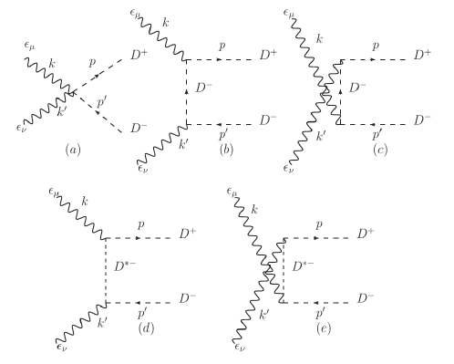
and , and represent the (or ), the (or ) and the photon fields, respectively. The Feynman rules can be derived from the interaction terms and they yield the Feynman diagrams for the process shown in Fig. 1. In the figure we also show the quadrimomenta of the incoming photons , and of the outgoing mesons , . The total amplitude is given by:
| (3) |
where
| (4) | ||||
| (5) | ||||
| (6) | ||||
| (7) | ||||
| (8) |
where and lag . We have introduced the Mandelstam variables of the elementary process, which are , and . As usual, we have included form factors, , in the vertices of the above amplitudes. We shall follow kk and use the monopole form factor given by
| (9) |
where is the 4-momentum of the exchanged meson and is a cut-off parameter. This choice has the advantage of yielding automatically and when the exchanged meson is on-shell. The above form is arbitrary but there is hope to improve this ingredient of the calculation using QCD sum rules to calculate the form factor, as done in ff , thereby reducing the uncertainties. Taking the square of the amplitude Eq. (3) and the average over the photon polarizations it is straigthforward to calculate the differential cross section:
| (10) |
In the center-of-mass reference frame we have and hence , and . It is then easy to see that:
| (11) |
Inserting Eq. (11) into Eq. (10) and using we find:
| (12) |
The angular integral can be done using the relations:
where is the angle between and . We emphasize that the only unknown in our calculation is the cut-off parameter . In what follows, we will determine it fitting our cross section to the LEP data on the process .
III Production of bound states
Now we describe the method to construct a bound state (denoted ) from the pair. As in pp1 , we impose phase space constraints on the mesons, forcing them to be “close together”. Here we do this through the prescription discussed in pes . The bound state is defined as
| (13) |
where is the bound state energy, is the relative three momentum between and in the state , are the energies of and and is the bound state wave function in momentum space, which has the following properties:
| (14) |
From Eq. (13), we can write the following relation between the amplitudes:
| (15) |
We assume that the and hence and also . Therefore the energy and the amplitude can be taken out of the integral. Moreover, since the binding energy is small we have and hence
| (16) |
With the amplitude above we calculate the cross section for bound state production:
| (17) |
where is the momentum of the produced bound state and is the flux factor. Now we will work in the center of mass frame of the collision, in which the momenta of the incoming photons may be different. In this frame we have
| (18) |
where and and are the energies of the colliding photons. The flux factor is then given by
| (19) |
Inserting this expression into Eq.(17) and integrating, the cross section reads
| (20) |
where we have used that .
To proceed with the calculation we need to know the bound state wave function at the origin . Fortunately, in go a similar bound state of open charm mesons was studied with the Bethe-Salpeter equation and an expression for the wave function was derived. In the first part of their paper the authors present a formalism which is general and can be adapted to our system. Formally, the Bethe-Salpeter equation reads , where is the two-body amplitude, is a matrix with elements which are the amplitudes of the transitions and which are calculated from a given effective Lagrangian. Finally is a loop function, which can be regularized with a cut-off. Here we will just quote the main formulas needed to calculate , which is given by
| (21) |
where
| (22) |
In the above expressions is the reduced mass (), is a cut-off parameter and is the binding energy. We shall follow mb and assume that GeV. From the above equations we see that one can compute the (dynamically generated) mass of a bound state and then determine its binding energy. Knowing , and fixing , we can use the above formulas to calculate . In what follows our reference value will be obtained using MeV and the mass of the bound state equal to MeV, as found in mb . With these numbers we get MeV and GeV3. These will be the values used to obtain all results, unless stated otherwise.
IV Equivalent photon approximation and the number of photons
The equivalent photon approximation is well known and it is described in several papers epa ; epa2 . In general, when the photon source is a nucleus one has to use form factors and the calculation becomes somewhat complicated. Here we will follow epa and define an UPC in momentum space. The distribution of equivalent photons generated by a moving particle with the charge is epa :
| (23) |
where , is the photon 4-momentum, is its transverse component, is the photon energy and is the Lorentz factor of the photon source ( and is the proton mass). To obtain the equivalent photon spectrum, one has to integrate this expression over the transverse momentum up to some value . The value of is given by , where is the radius of the projetile. For Pb, fm and hence GeV. After the integration over the photon transverse momentum the equivalent photon energy spectrum is given by:
| (24) |
Because of the approximations the above distribution is valid when the condition is fullfiled. Using Eq. (24) we can compute the cross sections of free pair production, , and of bound state production, . They are given by:
| (25) | ||||
| (26) |
where and are given by Eqs. (12) (with ) and (20) respectively.
V The low energy approximation
V.1 Free pairs
At low photon energies and close to the threshold, the produced mesons are non-relativistic and we can use the approximation in the heavy meson propagator, i.e.:
An analogous expression can be written for the propagator. From the above relation we can see that in this low energy regime the amplitudes with propagators are proportional to (Figs. 1b and 1c) and (Figs. 1d and 1e) and can be neglected when compared to the amplitudes without propagators, such as the one of the contact interaction in Fig. 1a. With this approximation the amplitude for production in the process is given by:
| (27) |
Taking the square and performing the average over the photon polarizations we have:
| (28) |
Inserting this amplitude into Eq. (10) we find:
| (29) |
Performing the integral over the solid angle and using the definitions and , we find
| (30) |
which is then substituted in Eq. (25) to give the final cross section for .
V.2 Bound states
In the low energy approximation the produced bound state is non-relativistic and then Eq. (16) reduces to:
| (31) |
Inserting Eq. (28) into the above equation and then using it in Eq. (20) we have:
| (32) |
Substituting the above expression into Eq. (26) and integrating we obtain the final analytical expression:
| (33) |
We emphasize that “low energy” here refers to the energy released by the projectiles, i.e. the invariant mass of the photon pair. The nuclear projectiles themselves may have very high energies.
 |
 |
| (a) | (b) |
 |
 |
 |
| (a) | (b) | (c) |
 |
 |
 |
| (a) | (b) | (c) |
VI Numerical results and discussion
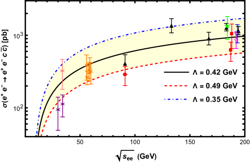
Having derived all the main formulas and discussed the numerical inputs, now we present our numerical results. In Fig. 2 we show the cross sections for free pair production and compare it to the existing experimental data from LEP lep . In fact, the LEP data are for , i.e., the measured final states are and . We assume that these two final states have the same cross section and, in order to compare with the data, we multiply our cross section by a factor two. In order to fit these data we will adapt expression (25) to electron-positron collisions. The cross section is same but the photon flux from the electron (and also from the positron) and the integration limits are different. The adaptation of Eq. (25) is performed in Appendix A. Comparing our formula with these data, we determine the only parameter in the calculation, which is the cut-off . In the figure, the curves are obtained substituting Eqs. (12) and (42) into (25). In the latter . We did not attempt to perform a least chi square fit. Instead we will carry on some uncertainty and work with the band GeV.
In Fig. 3 we show the cross section for production. The black solid lines show the result with our central parameter choice. Fig. 3a shows the sensitivity of the result to the value of . In Fig. 3b we vary the values of in the range defined in Fig. 2. In this sense we propagate the uncertainty from the fit of the data to our results. Taking this as the error in our result, the obtained cross section for the reaction at TeV is:
| (34) |
Assuming that the reaction has the same cross section as the one given above for charged states, the total cross section for charm production in photon-photon exclusive processes, we have
| (35) |
In Appendix B, using crude approximations, we have arrived at the following identity for inclusive cross sections:
| (36) |
This suggests that, for a given high energy, electromagnetic interactions in Pb-Pb are as efficient as strong interactions in p-p for charm production. Very recently, two independent analyses of the LHC data obtained estimates for the inclusive charm production cross section in proton proton collisions at TeV, which are dominated by the strong interaction. In yg the authors find:
| (37) |
and a quite similar result was obtained in lu . According to (36), (35) should be smaller (because it is exclusive) but of the order of magnitude of (37). Considering the uncertainties, we believe that this is approximately true.
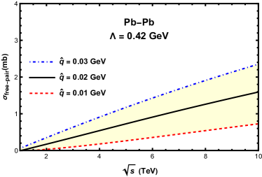
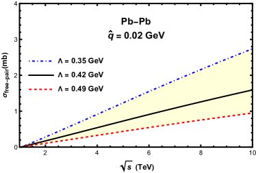
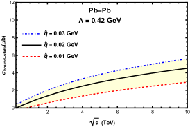
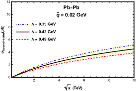
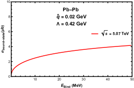
In Fig. 4 we present the cross section for bound state production and study its dependence on (Fig. 4a), on (Fig. 4b) and on the binding energy (Fig. 4c). As expected, it is much smaller than the cross section for open free pair production. However, it is encouraging to see that at TeV we have:
| (38) |
This number should be compared with results found in br and in fa . In those papers, the production cross section of scalar states and in Pb Pb ultra-peripheral collisions at TeV were calculated and the results were in the range
| (39) |
where stands for or . The works br and fa are relevant for us because there the states were also treated as molecules. However there is an important difference. In br and fa the authors used the Low formula, which connects the cross section with the decay width (used as input). In very few cases this width was measured and in some other very few cases the width was estimated with the help of a formalism valid for dynamically generated (and hence molecular) states. Here we propose a method to form the molecular state which is more general and independent of the knowledge of the decay width. Another difference is that the states and are significantly heavier than the molecule, whose mass is MeV. Moreover, in br and fa the equivalent photon calculation was done in the impact parameter space. In spite of these differences the obtained cross sections are of the same order of magnitude.
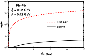
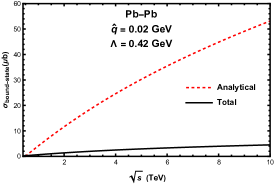
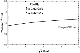
For completeness, in Fig. 5a we compare the cross sections for free pair and bound state production and in Fig. 5b we compare the exact numerical evaluation of with the approximate analytical expression, Eq.(33). We observe that the cross section obtained with the analytical formula is accurate only at low energies. At higher energies it becomes larger than the complete numerical formula. We can understand this behavior noticing that in Eq.(33) we assumed that both and the form factor did not depend on nor on at low energies and therefore resulted in a smaller denominator ( where it should have been ) and a constant argument of the form factor, which, as we can see from Fig. 4b, is crucial to our numerical results. Nevertheless, the exact and the analytical formula differ essentially only by a multiplicative factor close to 10. Dividing Eq. (33) by 10, it reproduces the exact formula within 20 % accuracy in the relevant LHC range and can thus be useful for practical applications. This is shown Fig. 5c.
To summarize, we have calculated, for the first time in the literature, the cross section for the production of a heavy meson molecule in ultra-peripheral collisions. We have combined a effective Lagrangian to compute the amplitude of the process with a prescription to project this amplitude onto the amplitude for bound state formation. The resulting cross section was then convoluted with the equivalent photon fluxes from the projetile and target and the final cross section was obtained. For TeV it is . This number is consistent with the results obtained for other scalar exotic charmonium molecules in br and fa . The parameters of the calculation are , and , which are the hadronic form factor cut-off, the maximum momentum of an emitted photon and the binding energy, respectively. All these parameters can be constrained by experimental information and by calculations. Thus, we believe that in the future it will be possible to increase the precision of our calculation.
Acknowledgements.
We are deeply indebted to K. Khemchandani and A. Martinez Torres for instructive discussions. This work was partially financed by the Brazilian funding agencies CNPq, CAPES, FAPESP, FAPERGS and INCT-FNA (process number 464898/2014-5). F.S.N. gratefully acknowledges the support from the Fundação de Amparo à Pesquisa do Estado de São Paulo (FAPESP). C.A.B. acknowledges support by the U.S. DOE Grant DE-FG02-08ER41533 and the Helmholtz Research Academy Hesse for FAIR.Appendix A Cross section of the process
In this appendix we will adapt Eq. (25) to the process. We start from Eq.(23) with :
| (40) |
First we recall that . Then we make the following change of variables:
After changing the variables we integrate Eq. (40) over :
| (41) |
The solution of this integral is:
| (42) |
After these changes in Eq. (25), we can write the cross section for the process inserting Eq. (42) into Eq. (25) and recalling that for electrons we use and also .
Appendix B in QED versus in QCD
In this paper we have been presenting predictions for quantities which are poorly known experimentally. In order to know, at least, what to expect and to have an idea of the order of magnitude of the cross sections we present below an estimate of the cross sections of the QED process and of the QCD process . The latter can be calculated with the simple convolution formula of the parton model:
| (43) |
where and are the proton momentum fractions of the colliding partons. In the above expression the integration limits come from the kinematical constraint . We know that this reaction is domintated by the elementary process . In a rough approximation the gluon momentum distributions and the elementary cross section are given by:
| (44) |
With these choices the integral above can be easily performed and yields:
| (45) |
In the case of charm production in an UPC of Pb-Pb we have an analogous convolution formula written in terms of the energies and of the colliding photons. Assuming that the maximum energy carried by one emitted photon is , the cross section is written as:
| (46) |
In the above expression the integration limits come from the kinematical constraint . The number of equivalent photons with energy , , and the photon-photon fusion cross section into an object with invariant mass can be roughly approximated by
| (47) |
We note the similarity between the above expressions and (44). As before this integral can be easily solved and we find:
| (48) |
Not surprisingly, (45) and (48) are identical except for the pre-factors. Using , and , we find
| (49) |
We could assume that , which is also a reasonable value. Then the above ratio would have been .
In Eq. (44) we could improve the approximation for . At increasingly higher energies the more singular behavior of the gluon distribution can be represented by , with . Analogously, in Eq. (47) we could improve the approximation for including the correction. This would change both cross sections in (49) in the same direction.
From this exercise we conclude that, for charm inclusive production at the same nucleon-nucleon center of mass energy, we have:
| (50) |
The above approximate identity is, of course, very crude but it tells us that the two reactions have comparable cross sections.
References
- (1) N. Brambilla, S. Eidelman, C. Hanhart, A. Nefediev, C.-P. Shen, C. E. Thomas, A. Vairo, and C.-Z. Yuan, Phys. Rept. 873, 1 (2020); R. M. Albuquerque, J. M. Dias, K. P. Khemchandani, A. Martinez Torres, F. S. Navarra, M. Nielsen and C. M. Zanetti, J. Phys. G 46, 093002 (2019).
- (2) L. Meng, B. Wang, G. J. Wang and S. L. Zhu, Phys. Rept. 1019, 1 (2023).
- (3) C. A. Bertulani, S. Klein and J. Nystrand, Ann. Rev. Nuc. Part. Sci. 55, 271 (2005).
- (4) D. Marietti, A. Pilloni and U. Tamponi, Phys. Rev. D 106, 094040 (2022). Pioneering studies were presented in S. J. Brodsky and F. S. Navarra, Phys. Lett. B 411, 152 (1997).
- (5) P. Artoisenet and E. Braaten, Phys. Rev. D 83, 014019 (2011); Phys. Rev. D 81, 114018 (2010); C. Bignamini, B. Grinstein, F. Piccinini, A. D. Polosa and C. Sabelli, Phys. Rev. Lett. 103, 162001 (2009).
- (6) A. Esposito, E. G. Ferreiro, A. Pilloni, A. D. Polosa and C. A. Salgado, Eur. Phys. J. C 81, 669 (2021)
- (7) H. Zhang, J. Liao, E. Wang, Q. Wang and H. Xing, Phys. Rev. Lett. 126, 012301 (2021); B. Wu, X. Du, M. Sibila and R. Rapp, Eur. Phys. J. A 57, 122 (2021).
- (8) D. Gamermann, E. Oset, D. Strottman, and M. J. Vicente Vacas, Phys. Rev. D 76, 074016 (2007).
- (9) J. Nieves and M. P. Valderrama, Phys. Rev. D 86, 056004 (2012).
- (10) C. Hidalgo-Duque, J. Nieves, and M. P. Valderrama, Phys. Rev. D 87, 076006 (2013).
- (11) S. Prelovsek, S. Collins, D. Mohler, M. Padmanath, and S. Piemonte, JHEP 06, 035 (2021).
- (12) D. Gamermann and E. Oset, Eur. Phys. J. A 36, 189 (2008).
- (13) P. Pakhlov et al. [Belle], Phys. Rev. Lett. 100, 202001 (2008).
- (14) K. Chilikin et al. (Belle), Phys. Rev. D 95, 112003 (2017).
- (15) E. Wang, W.-H. Liang, and E. Oset, Eur. Phys. J. A 57, 38 (2021).
- (16) E. Wang, H.-S. Li, W.-H. Liang, and E. Oset, Phys. Rev. D 103, 054008 (2021).
- (17) C. W. Xiao and E. Oset, Eur. Phys. J. A 49, 52 (2013).
- (18) O. Deineka, I. Danilkin, and M. Vanderhaeghen, Phys. Lett. B 827, 136982 (2022).
- (19) P. C. S. Brandão, J. Song, L. M. Abreu and E. Oset, Phys. Rev. D 108, 054004 (2023).
- (20) X. H. Cao, M. L. Du and F. K. Guo, [arXiv:2401.16112 [hep-ph]].
- (21) P. Lebiedowicz, O. Nachtmann and A. Szczurek, Phys. Rev. D 98, 014001 (2018).
- (22) M. E. Bracco, M. Chiapparini, F. S. Navarra and M. Nielsen, Prog. Part. Nucl. Phys. 67, 1019 (2012).
- (23) An introduction to quantum field theory, M. Peskin and M. Schroeder, Addison-Wesley (1996), p. 150.
- (24) D. Gamermann, J. Nieves, E. Oset and E. Ruiz Arriola, Phys. Rev. D 81, 014029 (2010).
- (25) C. A. Bertulani and G. Baur,Phys. Rept. 163, 299 (1988).
- (26) G. Baur, K. Hencken, D. Trautmann, S. Sadovsky and Y. Kharlov, Phys. Rept. 364, 359 (2002).
- (27) W. Da Silva [DELPHI], Nucl. Phys. B Proc. Suppl. 126, 185 (2004); A. Csilling [OPAL], AIP Conf. Proc. 571, 276 (2001). [arXiv:hep-ex/0010060 [hep-ex]].
- (28) Y. Yang and A. Geiser, PoS EPS-HEP2023, 367 (2024), arXiv:2311.07523 [hep-ph]].
- (29) C. Bierlich, J. Wilkinson, J. Sun, G. Manca, R. G. de Cassagnac and J. Otwinowski, arXiv:2311.11426 [hep-ph]].
- (30) B. D. Moreira, C. A. Bertulani, V. P. Goncalves and F. S. Navarra, Phys. Rev. D 94, 094024 (2016).
- (31) R. Fariello, D. Bhandari, C. A. Bertulani and F. S. Navarra, Phys. Rev. C 108, 044901 (2023).