2024 \publishedxx March 2018
Composite Effective Field Theory Signal from Anomalous Quartic Gauge Couplings for and Productions
Abstract
Parameterization of heavy effects beyond the Standard Model is available using higher-dimension operators of the effective field theory and their Wilson coefficients, where their values are not known. Experimental sensitivity to the Wilson coefficients can be significantly changed in case of the usage of composite anomalous signal, which contains anomalous contributions from background processes in addition to the conventional ones from the signal process. In this work, this approach is applied to the search for anomalous quartic gauge couplings with seven EFT operators in the electroweak production of and in collisions. For the majority of coefficients, sensitivity in the former channel is smaller than that in the latter one. However, it is shown, that composite anomalous signal affects production stronger than production, making sensitivities closer. One-dimensional limits on the Wilson coefficients are changed up to 27.3% and 9.7% due to the background anomalous contributions in and productions, respectively.
keywords:
Standard Model, effective field theory, vector boson scattering, quartic gauge coupling, collider experiment 10.31526/LHEP.2024.5191 Introduction
The Standard Model (SM) is a theory of elementary particle physics that describes experimental data in high energy physics well Erler:2019hds . The main aim of such modern experiments is to find out significant deviations from the SM (new physics) in order to determine the correct way for its extension. This extension is expected to explain all or some of the theoretical and experimental issues of the SM, such as gravitational interaction, dark matter and dark energy, and hierarchy problem.
Direct searches for the new particles gave no results at the moment Rappoccio:2018qxp ; ParticleDataGroup:2022pth , which indicates a growth of prospects of the indirect approach. It is based on looking for anomalous interactions of the already known particles. An effective field theory (EFT) Weinberg:1978kz ; Degrande:2012wf provides a convenient way to parameterize heavy new physics at the current experimental energy scale as anomalous couplings of the SM particles. Its Lagrangian has the following form:
| (1) |
where is dimension-four SM Lagrangian and is a dimension- addition, which is the sum over all dimension- EFT operators . Each operator is constructed out of the SM fields without gauge symmetry breaking and accompanied by a Wilson coefficient , where is the scale of new physics. In this work bosonic couplings are studied; therefore, odd-dimension operators are not valid since they contain fermion fields.
Anomalous quartic gauge couplings (aQGCs) are usually studied using dimension-eight operators, since dimension-six ones do not predict genuine aQGCs Eboli:2016kko ; Almeida:2020ylr . Basis of such operators contains three types of -conserving operators. This work uses a subset of the basis, which includes three T-family operators, constructed from the field strengths,
| (2) | |||
| (3) | |||
| (4) |
three M-family operators, constructed from both field strengths and Higgs doublets,
| (5) | |||
| (6) | |||
| (7) |
and one S-family operator, constructed from the Higgs doublet derivatives only,
| (8) |
If some physical process can be produced via an aQGC and the Lagrangian is parameterized by one EFT operator, its squared amplitude can be written as
| (9) | ||||
It contains three terms: SM, interference (linear) and quadratic. Non-SM terms are referred to as the anomalous contributions.
EFT is used in the analyses of experimental data to set the limits on the Wilson coefficients ATLAS:2017vqm ; CMS:2020ioi ; ATLAS:2020nlt ; ATLAS:2022nru . Often for this purpose, only the signal process is decomposed according to Eq. (9), whereas background processes are assumed to have the SM term only. Actually, background processes are also affected by nonzero Wilson coefficients and can have significant anomalous contributions to the analysis signal region. Therefore, usage of the anomalous signal, composed of signal and background anomalous contributions, can lead to the significant changes in the limits on Wilson coefficients. Previously this methodology was tested for and productions and four aQGC operators. Maximum improvement of the limits was found at 9.1% for coefficient Semushin:2022gbm ; Semushin:2022amw . In this work composite anomalous signal is examined for and productions. The latter one is studied using another event selection compared to the previous studies.
2 Physical model
Vector boson scattering (VBS) processes are the most sensitive to the aQGCs. In collisions VBS processes are an inherent part of the electroweak (EWK) production of two vector bosons and two jets. However, it is possible to enhance VBS production using special kinematic cuts. In this work, VBS production of and processes is studied. These processes are rare, the first one has not been observed in the considered decay channel yet ATLAS:2020nlt , whereas the second one has been observed using data from LHC Run II ATLAS:2021pdg .
The main background to the EWK production of and is partially QCD production of the same final states. Example Feynman diagrams for VBS, EWK non-VBS and QCD productions of two vector bosons and two jets are presented in Figure 1. Large backgrounds for EWK and productions come from and production respectively, where one lepton is produced outside of the detector acceptance. In channel production of is accounted as an additional background. The sum of all other backgrounds in both channels is not larger than the SM (EWK and QCD) contribution from the signal process, which is used as its estimation. This includes nonresonant background to production, minor backgrounds and backgrounds usually estimated directly from data, e.g. the ones caused by the misidentification of the electron as a photon Kurova:2023txz .

In order to model the physical processes, the Monte Carlo event generator MadGraph5_aMC@NLO Alwall:2014hca is used in this work for parton-level calculations. Hadronization, parton shower and underlying event are simulated using Pythia8 Sjostrand:2014zea . The response of the typical particle detector operating at the LHC for the simulated events is parameterized using Delphes3. Calculations of the event yields are made using integrated luminosity of 140 fb-1, collected by the ATLAS detector during LHC Run II ATLAS:2022hro .
After the detector simulation, VBS-enhanced event selection criteria based on the ATLAS studies of and productions ATLAS:2020nlt ; ATLAS:2022nru are applied, summarized in Table 2111The same coordination system as in the ATLAS studies ATLAS:2020nlt ; ATLAS:2022nru is used in this work. is the rapidity, and -centrality. Transverse momentum is measured in the plane that is transverse with respect to the beam pipe. is the magnitude of the missing transverse momentum , and event-based -significance .. Both ATLAS studies use object-based missing transverse energy significance (-significance). In this work, it was changed to the event-based one ATLAS:2018uid for the simplicity, and the cutting value was chosen to obtain similar SM signal efficiency as in the ATLAS studies. Moreover, for the channel, a cut GeV was added since the sensitivity to aQGCs is larger at high .
Event selection criteria for and channels. 2 leptons of the same flavors and opposite charges 1 photon, GeV GeV GeV GeV1/2 -signif. GeV1/2 GeV, GeV Lepton veto , GeV , GeV GeV, GeV GeV GeV
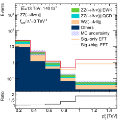
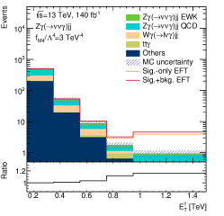
In addition to the signal process, some backgrounds can also have BSM contributions to the signal region. In this work, such backgrounds are and for and productions respectively. Additionally, BSM contributions from backgrounds , and were considered and found to be negligible; therefore they are not used in this work. Figure 2 presents distributions for the variables sensitive to aQGCs, for production and for production. SM contributions are shown using filled histograms, whereas solid lines represent EFT predictions for one Wilson coefficient. Usage of composite anomalous signal, i.e. signal and background anomalous contributions, increases predicted event yields, which lead to the improvement of the limits on the Wilson coefficient.
A possible issue in using the background BSM contributions can come from the fact that usually significant backgrounds are estimated using data, e.g., from the special control regions, enriched by the events of a specific background type. In this case, possible background BSM contributions can be included in its estimation. However, this can be avoided, if the control region is not sensitive to the aQGCs. Often this condition is satisfied since the control regions are usually enriched by the background SM events ATLAS:2022nru . Therefore, usually composite anomalous signal method can be used in real analyses.
3 Results
In this work, limits on the Wilson coefficients are set with the frequentist statistical method. Test statistic based on the likelihood ratio is used, and its distribution is assumed to be asymptotic; i.e., it corresponds to the chi-squared distribution with one or two degrees of freedom for one-dimensional limits or two-dimensional contours Wilks:1938dza ; Cowan:2010js . The likelihood function is constructed as a product of Poisson distributions for each bin from Figure 2 and Gaussian constraints for the nuisance parameters. In addition to the Monte Carlo modeling uncertainties, an additional systematic uncertainty of 20% is applied, which is typical for such kind of analyses ATLAS:2022nru . However, this does not make a significant contribution to the results.
Table 3 summarizes one-dimensional limits on the Wilson coefficients set with and without taking into account BSM contributions from backgrounds and for and productions respectively. It should be emphasized, that the limits on are set only using the channel since the corresponding operator does not affect quartic couplings with photons. The limits are set for two separate channels as well as for their combination. Improvement of the confidence interval is also presented and is significant even in the case of combination. Improvement of the limits on and in channel is smaller than the one obtained in Semushin:2022amw , which shows the dependence of the method on the event selection.
One-dimensional limits on the Wilson coefficients set with and without composite anomalous signal. Improvement of the confidence interval obtained with this method is shown in the last column. Coef. Sig.-only EFT Sig.+bkg. EFT Impr. [-0.238; 0.224] [-0.229; 0.216] 3.7% [-0.307; 0.305] [-0.259; 0.263] 14.8% [-0.586; 0.562] [-0.557; 0.534] 4.9% [-4.79; 4.78] [-3.48; 3.48] 27.3% [-6.89; 6.92] [-5.04; 5.05] 26.9% [-8.47; 8.47] [7.15; 7.15] 15.6% [-16.7; 16.7] [-13.4; 13.4] 19.6% [-0.103; 0.093] [-0.101; 0.092] 1.0% [-0.129; 0.127] [-0.120; 0.121] 6.2% [-0.097; 0.108] [-0.095; 0.106] 2.1% [-3.01; 3.03] [-2.72; 2.73] 9.7% [-2.35; 2.30] [-2.16; 2.12] 8.0% [-11.2; 11.2] [-10.3; 10.3] 8.4% Combination [-0.098; 0.089] [-0.097; 0.088] 1.3% [-0.123; 0.122] [-0.113; 0.115] 7.2% [-0.097; 0.107] [-0.095; 0.105] 2.1% [-2.71; 2.72] [-2.30; 2.31] 15.1% [-2.29; 2.25] [-2.07; 2.03] 9.7% [-7.27; 7.28] [-6.31; 6.31] 13.3%
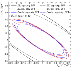
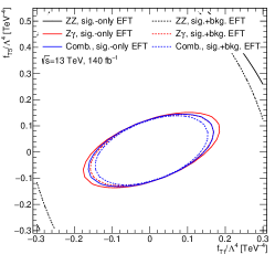
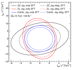
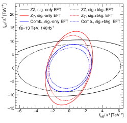
Two-dimensional limits are an additional illustration for the method of composite anomalous signals. Two-dimensional parameterization of the Lagrangian leads to the additional term compared to the decomposition from Eq. (9). This term, the so-called cross-term, represents interference between two EFT operators and can significantly change the sensitivity, so studies of two-dimensional limits are also important. In this work, two-dimensional limits are set for four pairs of the Wilson coefficients and presented in Figure 3. The largest improvement of the confidence regions is 40.0%, 18.6%, and 26.3% for , , and combined channel, respectively.
4 Conclusion
Application of the method of composite anomalous signal to the search for anomalous quartic gauge couplings in and productions in collisions is investigated in this work. In each channel, only one background has significant BSM contributions, and this allows improving one-dimensional limits on the Wilson coefficients up to 27.3%, 9.7% and 15.1% for production, production, and their combination, respectively. Significant improvement of these limits can lead to a sizeable improvement of the limits on new physics model parameters since model-independent and model-dependent approaches can be connected Remmen:2019cyz . Despite the fact that this work is made for an integral luminosity of 140 fb-1, this method is prospective to be used in the future, e.g., in LHC Run III data analyses, since it works independently on the luminosity growth.
Conflicts of interest
The authors declare that there are no conflicts of interest regarding the publication of this paper.
Acknowledgments
This work was supported by the Russian Science Foundation under grant 21-72-10113.
References
- [1] J. Erler and M. Schott, “Electroweak Precision Tests of the Standard Model after the Discovery of the Higgs Boson,” Prog. Part. Nucl. Phys. 106, 68-119 (2019).
- [2] S. Rappoccio, “The experimental status of direct searches for exotic physics beyond the standard model at the Large Hadron Collider,” Rev. Phys. 4, 100027 (2019).
- [3] R. L. Workman et al. [Particle Data Group], “Review of Particle Physics,” PTEP 2022, 083C01 (2022).
- [4] S. Weinberg, “Phenomenological Lagrangians,” Physica A 96, no.1-2, 327-340 (1979).
- [5] C. Degrande, N. Greiner, W. Kilian, O. Mattelaer, H. Mebane, T. Stelzer, S. Willenbrock and C. Zhang, “Effective Field Theory: A Modern Approach to Anomalous Couplings,” Annals Phys. 335, 21-32 (2013).
- [6] O. J. P. Éboli and M. C. Gonzalez-Garcia, “Classifying the bosonic quartic couplings,” Phys. Rev. D 93, no.9, 093013 (2016).
- [7] E. d. Almeida, O. J. P. Éboli and M. C. Gonzalez–Garcia, “Unitarity constraints on anomalous quartic couplings,” Phys. Rev. D 101, no.11, 113003 (2020).
- [8] M. Aaboud et al. [ATLAS], “Studies of production in association with a high-mass dijet system in collisions at 8 TeV with the ATLAS detector,” JHEP 07, 107 (2017).
- [9] A. M. Sirunyan et al. [CMS], “Measurement of the cross section for electroweak production of a Z boson, a photon and two jets in proton-proton collisions at 13 TeV and constraints on anomalous quartic couplings,” JHEP 06, 076 (2020).
- [10] G. Aad et al. [ATLAS], “Observation of electroweak production of two jets and a Z-boson pair,” Nature Phys. 19, no.2, 237-253 (2023).
- [11] G. Aad et al. [ATLAS], “Measurement of electroweak production and limits on anomalous quartic gauge couplings in pp collisions at = 13 TeV with the ATLAS detector,” JHEP 06, 082 (2023).
- [12] A. Semushin and E. Soldatov, “Methodology of accounting for aQGC effect on background for improvement of the limits on EFT coupling constants in case of electroweak production at the conditions of Run2 at the ATLAS experiment,” PoS PANIC2021, 127 (2022).
- [13] A. E. Semushin and E. Y. Soldatov, “Study of Corrections for Anomalous Coupling Limits Due to the Possible Background BSM Contributions,” Symmetry 14, no.10, 2082 (2022).
- [14] G. Aad et al. [ATLAS], “Observation of electroweak production of two jets in association with an isolated photon and missing transverse momentum, and search for a Higgs boson decaying into invisible particles at 13 TeV with the ATLAS detector,” Eur. Phys. J. C 82, no.2, 105 (2022).
- [15] A. Kurova, E. Soldatov and D. Zubov, “Estimation of Electron-to-Photon Misidentification Rate in Z() Measurements for Conditions of ATLAS Experiment during Run II,” Phys. Part. Nucl. 54, no.1, 227-231 (2023).
- [16] J. Alwall, R. Frederix, S. Frixione, V. Hirschi, F. Maltoni, O. Mattelaer, H. S. Shao, T. Stelzer, P. Torrielli and M. Zaro, “The automated computation of tree-level and next-to-leading order differential cross sections, and their matching to parton shower simulations,” JHEP 07, 079 (2014).
- [17] T. Sjöstrand, S. Ask, J. R. Christiansen, R. Corke, N. Desai, P. Ilten, S. Mrenna, S. Prestel, C. O. Rasmussen and P. Z. Skands, “An introduction to PYTHIA 8.2,” Comput. Phys. Commun. 191, 159-177 (2015).
- [18] J. de Favereau et al. [DELPHES 3], “DELPHES 3, A modular framework for fast simulation of a generic collider experiment,” JHEP 02, 057 (2014).
- [19] G. Aad et al. [ATLAS], “Luminosity determination in collisions at TeV using the ATLAS detector at the LHC,” Eur. Phys. J. C 83, no.10, 982 (2023).
- [20] G. Aad et al. [ATLAS], “Object-based missing transverse momentum significance in the ATLAS detector,” ATLAS-CONF-2018-038.
- [21] G. Cowan, K. Cranmer, E. Gross and O. Vitells, “Asymptotic formulae for likelihood-based tests of new physics,” Eur. Phys. J. C 71, 1554 (2011) [erratum: Eur. Phys. J. C 73, 2501 (2013)].
- [22] S. S. Wilks, “The Large-Sample Distribution of the Likelihood Ratio for Testing Composite Hypotheses,” Annals Math. Statist. 9, no.1, 60-62 (1938).
- [23] G. N. Remmen and N. L. Rodd, “Consistency of the Standard Model Effective Field Theory,” JHEP 12, 032 (2019).