An emergent cosmological model from running Newton constant
Abstract
We propose an emergent cosmological model rooted in the Asymptotically Safe antiscreening behavior of the Newton constant at Planckian energies. Distinguishing itself from prior approaches, our model encapsulates the variable nature of through a multiplicative coupling within the matter Lagrangian, characterized by a conserved energy-momentum tensor. The universe emerges from a quasi-de Sitter phase, transitioning to standard cosmological evolution post-Planck Era. Our analysis demonstrates the feasibility of constraining the transition scale to nearly classical cosmology using Cosmic Microwave Background (CMB) data and the potential to empirically probe the antiscreening trait of Newton’s constant, as predicted by Asymptotic Safety.
I Introduction
For decades, the standard model of cosmology has been very successful in describing the observable universe in accordance with experimental observations. We are currently living in an era of precision cosmology in which observations of the cosmic microwave background (CMB) Hinshaw et al. (2013); Akrami et al. (2020); Aghanim et al. (2020a, b, c), large scale structure (LSS) Tegmark et al. (2004); Seljak et al. (2005), type-IA supernovae (SNeIa) Perlmutter et al. (1999); Riess et al. (1998), baryon acoustic oscillation (BAO) Eisenstein et al. (2005), weak lensing Jain and Taylor (2003), gravitational waves (GW) Abbott et al. (2017) and more have allowed us to refine our picture of how the universe evolved by formulating, analyzing and potentially discarding theoretical models.
However, it is becoming increasingly clear that the picture is not complete and there are still important open problems and issues that need to be addressed. Among these the idea of inflation, although extremely successful, has recently been put under scrutiny. According to inflation, the universe is believed to have gone through a period of accelerated expansion at very early times Guth (1981); Linde (1982); Starobinsky (1980). This idea was proposed to address two problems, known as the horizon and flatness problems, that plagued the early theory. Besides solving two major problems, the success of the inflationary paradigm relies on modern observations that show how the initial conditions for the hot big bang can be produced during this period of inflation. The main breakthrough came when early CMB observations Hinshaw et al. (2013) detected a nearly scale-invariant power spectrum which can be perfectly explained by inflation. Later observations from Planck made constraints on the model very strong, thus allowing to discard inflationary models that do not fit the observations. The latest Planck data favors single-field scalar models of inflation with concave potential coupled to General Relativity (GR). The data also prefers no significant departure from slow-roll behavior Akrami et al. (2020). Still, the nature of the inflationary scalar field is not known at present. Therefore other models for inflation and the behavior of the universe in the early stages have been proposed over the years. Some of these models are able to address the same issue and produce a scale-invariant CMB power spectrum. For example, bouncing scenarios and ekpyrotic models have been suggested as possible alternatives to inflation Cai et al. (2010); Battefeld and Peter (2015); Lyth and Wands (2002); Brandenberger and Peter (2017). This shows that there is room for other viable models of the universe to be proposed and there are stringent quantitative tests that can be made to constrain such proposals.
In the present article, we propose a minimal modification to GR at UV scales inspired by the Asymptotic Safety (AS) paradigm Bonanno (2023) and implemented through a multiplicative coupling of matter to gravity as proposed in Markov and Mukhanov (1985). This proposal provides a relation between a variable Newton coupling and variable and does not involve any additional unknown fields. Hence we show that the quasi-de Sitter phase in the early universe can be obtained as a result of the Asymptotically Safe nature of gravity at high energies. We show that this new mechanism achieves the same results as scalar field inflation and we provide arguments in support of the fact that it can also produce a scale-invariant CMB power spectrum.
The current proposal diverges from prior investigations into Renormalization Group (RG) improved cosmologies Bonanno and Reuter (2002a, b); Cai and Easson (2011) by adopting a Lagrangian approach, thus preserving diffeomorphism invariance. While it shares conceptual similarities with the framework introduced in Bonanno (2012), and subsequently elaborated upon in various studies (cf. Bonanno and Saueressig (2017) for an overview), it avoids imposing a cutoff identification based on curvature invariants Bonanno et al. (2018). Recent findings, notably those derived from the fluctuation approach Pawlowski and Reichert (2021); Bonanno et al. (2022), illustrate that the behavior of the Newton constant during high-energy scattering processes is predominantly governed by the external graviton momenta which should scale in accordance with the energy density of the system. A promising initial result stemming from this novel perspective is evidenced in the regular black hole collapse model discussed in Bonanno et al. (2023).
The article is organized in the following way: In section II we briefly discuss AS gravity with the non trivial matter-gravity coupling and apply the formalism to a Friedmann universe in section III. Implications of the model for the early universe and the correspondence between the proposed model and scalar field inflation are discussed in section IV. Finally results and future perspectives are summarized in section V. Throughout the article, we make use of units with (unless explicitly stated) and metric signature .
II Field equations and energy momentum


We aim to build a cosmological model based on three main assumptions regarding the fundamental behavior of gravity at high energies:
-
(i)
There exists a non-minimal matter-gravity coupling that depends on the energy scale as suggested by Markov and Mukhanov (MM) in Markov and Mukhanov (1985).
-
(ii)
The precise form of as a function of the energy density can be obtained from the running of in Asymptotic Safety under a physically motivated cut-off identification.
-
(iii)
The running of alone captures the qualitative physical features of the model, i.e. we do not explicitly include possible effects from the running of higher dimensional operators, cosmological constant, or matter fields.
We do not wish to add any additional matter fields besides a standard one such as dust, radiation or a stiff fluid and the accelerated expansion phase in the early universe, namely inflation, shall be recovered from the matter-gravity coupling. Of course, at low energies we must retrieve the standard field equations of GR. With the above assumptions the field equations can be derived in the MM prescription from the following action
| (1) |
where is the determinant of the spacetime metric , is the matter Lagrangian and the matter-gravity coupling depends only on a scalar function of the matter-energy density Markov and Mukhanov (1985). Variation of the matter part of the action, with respect to the metric leads to
| (2) |
and the variation of the full action leads to the modified Einstein equations
| (3) |
where
| (4) |
is the effective energy-momentum tensor while
| (5) |
is the energy-momentum tensor for a perfect fluid, where is the fluid’s pressure which we assume may be obtained from an equation of state . Looking at Eq. (3) and(4) we can identify the terms
| (6) |
as a running gravitational constant and a running cosmological constant . In order to retrieve GR at low densities, for we must ensure that as we get , which implies .
Consider a matter fluid of proper density , 4-velocity with and rest mass density . Mass continuity implies
| (7) |
and for a non-dissipative fluid, we have
| (8) |
The effective stress-energy tensor needs to be conserved, i.e.
| (9) |
To see how the effective energy density evolves, we can project it along the four-velocity field which gives
| (10) |
where the quantities with tilde are the effective fluid’s energy-density and pressure that can be obtained from Eq. (4) as
| (11) | |||||
| (12) |
Now we can examine the weak and strong energy conditions for the effective fluid. The weak energy condition (w.e.c.) for the perfect fluid in (5) holds if and . Then for the effective quantities the w.e.c. is
| (13) |
which can be written as
| (14) |
Notice that the behavior of determines the validity of the w.e.c. for the effective fluid. In particular if the w.e.c. holds for the fluid and we always have that , while may become negative if . A similar reasoning holds for the strong energy condition (s.e.c.) which for the perfect fluid in (5) corresponds to and (with being the spatial directions). The s.e.c. for the effective fluid is then given as
| (15) |
which can be written in terms of the classical fluid components as
| (16) |
Notice that the condition must be violated in order to have a phase of accelerated expansion. Then the first of Eq. (16) provides a condition on for which the s.e.c. holds for the classical fluid but is violated for the effective fluid.
The above framework provides a scenario for a variable cosmological constant that naturally emerges from the matter-gravity coupling. The only available freedom is in the choice of one of the two functions and . In the following, we aim to build a model for the early universe for which the gravitational coupling is prescribed from the Asymptotic Safety (AS) program and therefore we will fix the function from the AS paradigm and obtain and accordingly.
If gravity is renormalizable around a non-Gaussian fixed point, one would expect that at very high energies, with being the characteristic scale of energy at which the physics is being probed Reuter (1998); Weinberg (1980); Eichhorn (2019); Pawlowski and Reichert (2021); Reichert (2020); Reuter and Saueressig (2019); Percacci (2017); Bonanno et al. (2020a); Bonanno et al. (2022); Bonanno et al. (2020b). Then the variable Newton coupling can be taken as a function of this characteristic energy scale as Bonanno et al. (2022)
| (17) |
where the scale is model dependent while is the UV fixed point. To connect the cutoff scale and the energy density , we follow the prescription discussed in Bonanno et al. (2020a); Platania (2019); Bonanno et al. (2023). Thus we consider the simplest relation between and involving both Newton’s and Planck constants which can be obtained from dimensional analysis. This is
| (18) |
from which we obtain the following form for :
| (19) |
where is a dimensional parameter in which we absorb and the other constants. The information on the cutoff scale is now encoded in which we can interpret as a crossover scale separating the Reuter fixed point from the Gaussian fixed point: when the dynamics of the system is essentially determined by the vanishing of the effective coupling constant. In the opposite limit, standard gravity is recovered. From Eq. (19) we obtain the expressions for and Bonanno et al. (2023):
| (20) | |||||
| (21) |
Notice that for we get and thus retrieving the classical GR limit. However for large we see that while diverges. Looking at Eq. (20) we can also see that as diverges diverges as well but more slowly.
III Cosmology
The evolution of the universe is governed by the Friedmann equations. We start by considering a Friedmann-Robertson-Walker (FRW) universe with metric
| (22) |
where is the scale factor, is the curvature and is the line element on the unit sphere. The Friedmann equations for the AS model with MM prescription are then obtained from the metric (22) with the effective energy-momentum tensor (4) as
| (23) | |||||
| (24) | |||||
where is the Hubble parameter. Then, the evolution of the effective energy density can be easily obtained from Eq. (10) as
| (25) |
Since at all times, from the above equation we see that the effective energy momentum is conserved if the original energy momentum is. Namely Eq. (10) holds if
| (26) |
In the limit, (and for ), both Friedmann equations of our model reduce to the standard Friedmann equations of GR
| (27) | |||||
| (28) |
On the other hand, at high energies, i.e. for , the function goes to zero in such a way that we obtain a de Sitter-like initial phase for the early universe.
In the following, we will consider a matter content given by a perfect fluid described by a linear barotropic equation of state (e.o.s.) , and we will pay particular attention to the cases of non relativistic matter (including both baryonic and dark matter) for which , radiation for which and a stiff fluid for which . The case for a stiff equation of state in the early universe was originally proposed by Zel’dovich Zel’dovich (1961); Zeldovich (1972) in order to describe a big bang scenario for a universe filled with hot baryons. More recently the same idea has been reevaluated in the context of a universe with a polytropic ‘dark fluid’ where the internal energy plays the role of a stiff fluid and dominates at early times Chavanis (2015). Interestingly, in our model, due to the vanishing of the gravitation coupling , the qualitative behavior of the cosmological model at high densities does not depend on the specific fluid model, with the e.o.s. being important in the determination of the energy scales at which the AS corrections become relevant.


We can now take the universe age today as and set . In the left panel of Fig. 1, we show the effective energy density for a single fluid (denoted by the subscript ) in the three cases mentioned above (i.e. ) as a function of the scale factor . The classical energy density is obtained from integration of the conservation equation as and is given by Eq. (20). Then for each fluid component of the universe, we define with being the energy density for which the universe is flat, namely . Then in terms of the e.o.s. parameter we can write the first Friedmann equation in the following way
| (29) |
with
| (30) | |||||
| (31) |
where are the current values of the density parameters of the respective fluids and is the energy density for the universe to be flat today. To compare the behavior of the scale factor in the CDM and AS models, we solve the Friedmann Eq. (29) numerically assuming the fiducial cosmological parameters from Aghanim et al. (2020b) to find with the initial condition . The resulting scale factor is shown in the right panel of Figure 1 with a ratio of fixed arbitrarily at for illustrative purposes. We see that at late times the model follows the standard CDM behavior, while at early times the scale factor never reaches zero and asymptotically decreases to with , thus showing that the big bang singularity is avoided and there is an infinite amount of time in the past for the universe to reach thermal equilibrium.
We are interested in the behavior of at high energies, i.e. , with the aim of replacing inflation driven by a scalar field with an exponential expansion driven by the variable in AS. This can be accomplished since the model automatically leads to a quasi-de Sitter phase for and no singularity is present at any finite co-moving time. The condition for accelerated expansion from Eq. (24) implies which, according to Eq. (16), for a universe dominated by a single fluid with the equation of state, becomes
| (32) |
We plot this condition as a function of the energy density in the left panel of Fig. 2 for dust, radiation and stiff fluid. We can clearly see from the figure that is satisfied as for all fluid models. We also see that the qualitative behavior for large densities is the same regardless of the fluid model and the e.o.s. plays a role only in determining the energy scale at which becomes negative. To understand this better we can look at how the effective equation of state relating to behaves in the early universe. The effective equation of state parameter is defined as
| (33) |
If , as is the case for Eq. (20), then for large we see that the effective equation of state behaves as
| (34) |
for any value of . This proves that at high energies, i.e. in the very early universe, the effective equation of state parameter shows a limiting de Sitter behavior regardless of the value of . We show the parameter in the right panel of Fig. 2 for the cases of dust (), radiation () and stiff fluid (). From the figure, we can also see that at low energies the fluids behave as ordinary perfect fluids.
To see how the cosmological model in AS solves the flatness problem, we can use the Friedmann equations (23) and (24) to write
| (35) |
where is the effective density parameter. We can clearly see that is a stable solution since as in AS. This can also be seen easily by introducing small perturbations to the density parameter of the form with . At the linear order, Eq. (35) becomes
| (36) |
Solving this differential equation in a regime where yields the following result,
| (37) |
Again, since during the AS phase in the early universe, the perturbations decay and the flat solution is stable.
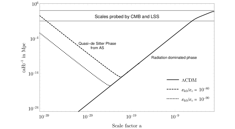
To show that this model also solves the horizon problem we compare the evolution of the comoving Hubble radius in the AS cosmological model with that of the standard CDM model. In the standard CDM model without an inflationary phase, the amount of conformal time between the initial singularity and the formation of the CMB is much smaller than the conformal age of the universe today. This leads to patches of angular size on the all-sky projection of the CMB to be causally disconnected. However, the CMB appears to have a uniform temperature map, thus suggesting that those same patches were in causal contact before the emission of the CMB. Adding a phase of exponential expansion to the CDM model before the hot Big Bang solves the problem. To see this we just need to notice that a decreasing comoving Hubble radius during such a phase, corresponding to increasing the amount of conformal time in the early universe, allows for the past light cones of two points on the CMB to be in causal contact in their past (see Fig. 3).
In the AS model, this quasi-de Sitter phase is achieved automatically via the coupling of to . In Fig. 3 we show the evolution of the comoving Hubble radius with the Hubble parameter given by the first Friedmann equation (29). It can be clearly seen that in the early universe, during the quasi-de Sitter phase, the comoving Hubble radius was decreasing. The size of the universe at the time of the transition from the exponential expansion to a universe dominated by matter (such as radiation as considered in the figure) depends on the ratio between the current energy density () of the universe and the critical, model dependent, density of AS, namely . The transition from radiation-dominated to the matter-dominated epoch instead occurs around the recombination era and it follows the standard CDM behavior, regardless of the value of (as can be seen from the inflexion of the solid line at the top right of Fig. 3). For comparison, in the same figure, we also show the comoving Hubble radius for the standard CDM model.
IV Modelling the early universe
In order to compare the predictions of the AS model with those of a standard inflationary scenario we need to look at the Hubble slow-roll parameters which indicate the conditions for a sustained inflationary period in the early universe. The Hubble slow-roll parameters are given by Baumann (2022); Lyth and Riotto (1999)
| (38) |
where refers to the number of e-folds during inflation. The first condition is and it states that the fractional change of the Hubble parameter per e-fold has to be small. The second condition is , which on the other hand requires to remain small over a large enough number of Hubble times Baumann (2022). For AS cosmology we get
| (39) | |||||
The behaviors of and for an AS cosmological model with only radiation are shown in Fig. 4. We can see from the plot that at high energy densities, i.e. as we approach the very early universe, these Hubble slow-roll parameters become smaller than unity which signifies a sustained period of inflation. Notice that from Eqs. (39) and (IV) we see that for , corresponding to , we have that and both go to zero.

Now we would like to obtain constraints on the critical density parameter by using observational bounds from the primordial power spectrum generated by curvature perturbations during the inflationary period. This analysis will not only enable us to estimate some realistic values of the characteristic energy scale, but will also allow us to test the observational viability of the AS program of quantum gravity.
The first step in this direction involves the calculation of the two most important inflationary variables, e.g., the spectral index of scalar curvature perturbations and the ratio of tensor-to-scalar perturbations , in terms of the model parameters Mukhanov (2005). These two quantities are important because their values depend on the energy density scale at the onset of inflation and they can be constrained from observations of the CMB power spectrum. Usually, most inflationary models are constructed with one or more scalar fields with some potentials and canonical or non-canonical kinetic terms (see for example Lyth and Riotto (1999)). The inflationary observables are then expressed approximately in terms of the slow-roll parameters which in turn can be represented by the potential and its derivatives with respect to the scalar field .
However, our model of inflation in the AS framework is expressed in terms of an effective fluid. It is known that there is a correspondence between scalar field and fluid models Arroja and Sasaki (2010); Faraoni (2012); Mukhanov (2013) and therefore in order to write the inflationary observables in terms of our model parameters we shall consider the fluid description of inflation following the procedure suggested in Bamba et al. (2014a, b); Bamba and Odintsov (2016). To this aim in the following we will express the slow-roll parameters and in terms of fluid parameters by relating them to the Hubble parameter and its derivatives with respect to the number of e-folds during inflation. Then and can be directly related to the inflationary observables and from their definition in the scalar field case. A very important caveat is in order at this point. As we evaluate and from the analogy between fluids and scalar fields we need to keep in mind that while the correspondence is valid at the background level (namely for the FRW metric) the perturbations may turn out to be different in the two cases. In a model of slow-roll inflation however we may expect differences to remain small.
IV.1 Spectral index and tensor to scalar ratio for scalar field inflation
First, we briefly review how and are defined in terms of and in a model of inflation driven by a scalar field . The action of the scalar field with the Einstein-Hilbert term is given by
| (41) |
For slow-roll inflation the spectral index of curvature perturbations and the tensor-to-scalar ratio of density perturbations are given by Lyth and Riotto (1999)
| (42) |
The slow-roll parameters and can be defined in terms of the scalar field potential and its derivatives as
| (43) |
Now we redefine the scalar field in terms of a new scalar field , that later we identify as the number of e-folds during inflation so that the slow-roll parameters are written in terms of the redefined variable as
| (44) | |||||
| (45) |
where the primes denote derivatives with respect to the argument of the function on which the prime operates and .
If we consider a flat FRW universe with the metric (22) the Friedmann equations (46) and (47) during inflation become
| (46) | |||||
| (47) |
and they can be rewritten terms of the redefined scalar field as Bamba and Odintsov (2016)
| (48) | |||||
| (49) | |||||
where the number of e-folds during inflation is
| (50) |
and the subscripts and denote the beginning and end of inflation. Thus inverting Eqs. (48) and (49) we can now express and in terms of as
| (51) | |||||
| (52) |
Now using Eqs.(51)-(52), the slow-roll parameters in Eq.(44) and (45) can be written in terms of and its derivatives with respect to . Then and can be easily derived from Eqs. (42). The advantage of writing and in terms of is that we can now obtain the same quantities for the AS model for which the early universe is described by an effective fluid instead of a scalar field. The full expressions for the slow-roll parameters are given in Appendix A.
IV.2 Spectral index and tensor to scalar ratio in AS
We have seen that the slow roll approximation holds for the AS cosmological model. Also, as mentioned, it is well known that there is a correspondence between fluid models and scalar field inflation. Therefore at the background level, it makes sense to use the tools of scalar field inflation discussed in the previous subsection to obtain some indication of our model’s implications for the early universe. However, we must remember that even though the correspondence between the effective fluid model and the scalar field is valid at the background level this does not necessarily imply that there will be a correspondence between the quantities obtained at the perturbative level. Nevertheless, in the slow roll limit, with all higher order quantities being small, we may expect that the departure between the two approaches at a perturbative level will also remain small and therefore we may estimate and for the AS model using the tools discussed above. Our aim here is to express and in terms of for the AS cosmological model. Using the effective density and pressure from Eqs. (11) and (12) we can write the effective e.o.s. as
| (53) |
where . Without any loss of generality, we can express this effective e.o.s. as
| (54) |
where the effective pressure and density are functions of the number of e-folds . For a flat FRW universe, with , the Friedmann equations (23) and (24) can be rewritten as
| (55) | |||||
| (56) |
Using the continuity equation we obtain
| (57) |
where the primes denote derivatives with respect to the number of e-folds. Now we take the derivative of Eq. (56) and use the above relations to get
| (58) |
Now using Eq.(55), (56) and (58) we can express the slow-roll and the observational parameters in terms of the quantities describing the fluid, namely and . We report the explicit forms of the slow-roll parameters in Appendix A.
For some simple estimates, we can write the expressions for inflationary observables in the limit when and both vary slowly during the inflationary period, such that . It is straightforward to check that this condition corresponds to and consequently a slowly varying Hubble parameter . In this approximation, the observables take the simple form
| (59) |
These expressions can now be used to put constraints from observational data on the value of at the time of inflation.
IV.3 Constraints from observations
| () | GeV4 | GeV4 | GeV | GeV | |||
|---|---|---|---|---|---|---|---|
| 1/3 | (0.965, 0.13) | 57.62 | |||||
| (0.975, 0.10) | 78.08 | ||||||
| 1 | (0.965, 0.13) | 57.51 | |||||
| (0.975, 0.10) | 78.23 |
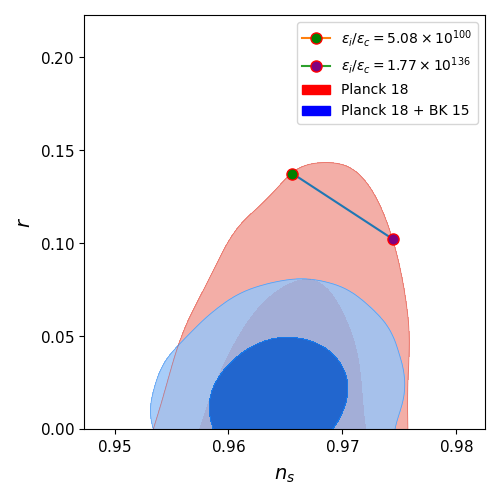
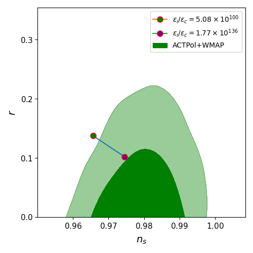
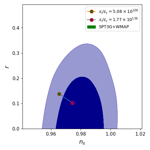
To compare our model of inflation in AS with current observational data we consider data sets obtained from Planck and other observations. We specifically consider the observational constraints on the scalar spectral index and the tensor-to-scalar ratio based on the Planck 2018 and BICEP2/Keck-Array 2015 (Planck 18 + BK 15) combined data sets Aghanim et al. (2020a, b, c); Akrami et al. (2020); Ade et al. (2018), the Atacama Cosmology Telescope DR4 likelihood combined with the WMAP satellite data (ACTPol+WMAP) Aiola et al. (2020); Hinshaw et al. (2013); Forconi et al. (2021) and the South-Pole Telescope polarization measurements combined with the WMAP satellite data (SPT3G+WMAP) Dutcher et al. (2021); Hinshaw et al. (2013); Forconi et al. (2021). Planck temperature, polarization, and lensing data have determined the spectral index of scalar perturbations to be at confidence level (CL) with no evidence of a scale dependence. On the other hand, the Planck data (Planck TT,TE,EE+lensing+lowEB) puts a CL upper limit on the tensor-to-scalar ratio, which is further improved by combining with the BICEP2/Keck Array data to obtain Aghanim et al. (2020b); Akrami et al. (2020). These are the strongest constraints on and to date.
Now, let us have a look at the explicit expression for to find allowed values of
| (60) |
If we use Eq. (59) to calculate and for our model, then having gives and , where the quantities with subscript i are evaluated at the horizon exit. Notice that, in view of the fact that for from Eq. (19) we get , we need in order to achieve the de Sitter phase for which . For example, for a critical density of the order of Planck density, , the energy scale of the universe at the horizon exit would have to be above the Planck density, i.e. corresponding to .
We plot the marginalized contours of and for the datasets considered along with the predictions of the AS model with radiation in Fig. 5. We can see that our model agrees well with all three datasets. In all three plots of Fig. 5, varies along the straight line with the points at the ends taking values and (assuming ). Similarly, we can obtain the constraints on the energy scales of inflation for the stiff fluid model as and . These values, together with the corresponding number of e-folds during the inflation period, are shown in Table 1 for both radiation and stiff fluid.
The number of e-folds from the time of horizon exit to the end of the quasi-de Sitter period is given by
| (61) |
Here and are the values of the scale factor at the moment of horizon exit and the end of the quasi-de Sitter period. The end of accelerated expansion is defined by . We then use Eq. (25) to write
| (62) |
where and are the energy densities at the moment of horizon exit and the end of the quasi-de Sitter period. Using the above equation, the number of e-folds becomes
| (63) |
To derive the ratio of energy densities at the two epochs, we use the constraints we obtained from CMB observations to find and the condition for the end of accelerated expansion to find . First, from the CMB constraints discussed above, we found that the ratio that gives , for radiation () is
| (64) |
Then from the condition which holds at the end of accelerated expansion, we get
| (65) |
These two equations give the ratio of the energy density at the horizon exit and the end of the quasi-de Sitter period
| (66) |
from which we can calculate the number of e-folds using Eq. (63), which gives
| (67) |
Similarly, we can perform the same calculations for dust and stiff fluid, for which the numbers of e-folds are
| (68) | ||||
Similar calculations for the ratio that gives , for the three matter models give . The values are consistent with the estimates of from scalar field inflation thus confirming that the model can be considered a viable alternative to standard inflationary models.
V Summary and Discussions
We considered a modification of the standard cosmological model at high densities that allows for a phase of accelerated expansion without the introduction of additional fields. This was achieved with the introduction of a matter-gravity coupling in the action that leads to an effective theory with varying gravitational coupling and in the field equations 111It is worth noting that due to the monotonic behavior of the coupling , we can not use the Markov-Mukhanov mechanism to explain the observed late-time acceleration of the universe within a single framework. There exist other approaches to variable and that attempts at explaining the late-time acceleration, see e.g. de Cesare et al. (2016).. We showed that the choice of consistent with the Asymptotic Safety paradigm allows us to reproduce a phase of accelerated expansion in the early universe without the aid of an ad hoc scalar field. We showed that there are ranges of values for , with and being the energy density at the horizon exit and the critical energy density (the model’s only free parameter) respectively, for which the observational constraints from the CMB data can be satisfied.
In the present work the constraints are derived assuming the equivalence between our effective fluid description and a scalar field model of inflation. However, an in-depth analysis of the quantum perturbations of the effective fluid during the inflationary period is necessary in order to properly put constraints on the model’s parameter. Such an analysis should also allow us to distinguish between our model and other existing models of inflation derived from particle physics or alternative theories. We plan to explore this direction in the future. Finally, we expect that the data obtained from future experiments such as CMB-S4 Abazajian et al. (2022); Zegeye et al. (2023), LiteBird Allys et al. (2023), CORE Delabrouille et al. (2018), CMB-Bhārat Adak et al. (2022), etc. will be able to test the validity of the model presented here.
Acknowledgement
AZ would like to thank Catania Astrophysical Observatory - INAF- for its warm hospitality during the preparation of the manuscript. DM, HC and AZ acknowledge support from Nazarbayev University Faculty Development Competitive Research Grant No. 11022021FD2926. The authors thank William Giarè and his group for giving us access to some of the data products used in this article. The authors also thank Antonio De Felice for useful comments and discussions.
Appendix A Slow-roll parameters and Inflationary Observables
Here we express and in terms of and its derivatives with respect to .
| (69) | |||||
| (70) | |||||
The slow-roll parameters in terms of and in the AS model are
| (71) | |||||
| (72) | |||||
References
- Hinshaw et al. (2013) G. Hinshaw et al. (WMAP), Astrophys. J. Suppl. 208, 19 (2013), eprint 1212.5226.
- Akrami et al. (2020) Y. Akrami et al. (Planck), Astron. Astrophys. 641, A10 (2020), eprint 1807.06211.
- Aghanim et al. (2020a) N. Aghanim et al. (Planck), Astron. Astrophys. 641, A1 (2020a), eprint 1807.06205.
- Aghanim et al. (2020b) N. Aghanim et al. (Planck), Astron. Astrophys. 641, A6 (2020b), [Erratum: Astron.Astrophys. 652, C4 (2021)], eprint 1807.06209.
- Aghanim et al. (2020c) N. Aghanim et al. (Planck), Astron. Astrophys. 641, A5 (2020c), eprint 1907.12875.
- Tegmark et al. (2004) M. Tegmark et al. (SDSS), Phys. Rev. D 69, 103501 (2004), eprint astro-ph/0310723.
- Seljak et al. (2005) U. Seljak et al. (SDSS), Phys. Rev. D 71, 103515 (2005), eprint astro-ph/0407372.
- Perlmutter et al. (1999) S. Perlmutter et al. (Supernova Cosmology Project), Astrophys. J. 517, 565 (1999), eprint astro-ph/9812133.
- Riess et al. (1998) A. G. Riess et al. (Supernova Search Team), Astron. J. 116, 1009 (1998), eprint astro-ph/9805201.
- Eisenstein et al. (2005) D. J. Eisenstein et al. (SDSS), Astrophys. J. 633, 560 (2005), eprint astro-ph/0501171.
- Jain and Taylor (2003) B. Jain and A. Taylor, Phys. Rev. Lett. 91, 141302 (2003), eprint astro-ph/0306046.
- Abbott et al. (2017) B. P. Abbott et al. (LIGO Scientific, Virgo, 1M2H, Dark Energy Camera GW-E, DES, DLT40, Las Cumbres Observatory, VINROUGE, MASTER), Nature 551, 85 (2017), eprint 1710.05835.
- Guth (1981) A. H. Guth, Phys. Rev. D 23, 347 (1981).
- Linde (1982) A. D. Linde, Phys. Lett. B 108, 389 (1982).
- Starobinsky (1980) A. A. Starobinsky, Phys. Lett. B 91, 99 (1980).
- Cai et al. (2010) Y.-F. Cai, E. N. Saridakis, M. R. Setare, and J.-Q. Xia, Phys. Rept. 493, 1 (2010), eprint 0909.2776.
- Battefeld and Peter (2015) D. Battefeld and P. Peter, Phys. Rept. 571, 1 (2015), eprint 1406.2790.
- Lyth and Wands (2002) D. H. Lyth and D. Wands, Phys. Lett. B 524, 5 (2002), eprint hep-ph/0110002.
- Brandenberger and Peter (2017) R. Brandenberger and P. Peter, Found. Phys. 47, 797 (2017), eprint 1603.05834.
- Bonanno (2023) A. Bonanno, Asymptotic Safety and Cosmology (Springer Nature Singapore, Singapore, 2023), pp. 1–27, ISBN 978-981-19-3079-9, URL https://doi.org/10.1007/978-981-19-3079-9_23-1.
- Markov and Mukhanov (1985) M. A. Markov and V. F. Mukhanov, Nuovo Cim. B 86, 97 (1985).
- Bonanno and Reuter (2002a) A. Bonanno and M. Reuter, Phys. Rev. D 65, 043508 (2002a), eprint hep-th/0106133.
- Bonanno and Reuter (2002b) A. Bonanno and M. Reuter, Phys. Lett. B 527, 9 (2002b), eprint astro-ph/0106468.
- Cai and Easson (2011) Y.-F. Cai and D. A. Easson, Phys. Rev. D 84, 103502 (2011), eprint 1107.5815.
- Bonanno (2012) A. Bonanno, Phys. Rev. D 85, 081503 (2012), eprint 1203.1962.
- Bonanno and Saueressig (2017) A. Bonanno and F. Saueressig, Comptes Rendus Physique 18, 254 (2017), eprint 1702.04137.
- Bonanno et al. (2018) A. Bonanno, A. Platania, and F. Saueressig, Phys. Lett. B 784, 229 (2018), eprint 1803.02355.
- Pawlowski and Reichert (2021) J. M. Pawlowski and M. Reichert, Front. in Phys. 8, 551848 (2021), eprint 2007.10353.
- Bonanno et al. (2022) A. Bonanno, T. Denz, J. M. Pawlowski, and M. Reichert, SciPost Phys. 12, 001 (2022), eprint 2102.02217.
- Bonanno et al. (2023) A. Bonanno, D. Malafarina, and A. Panassiti (2023), eprint 2308.10890.
- Reuter (1998) M. Reuter, Phys. Rev. D 57, 971 (1998), eprint hep-th/9605030.
- Weinberg (1980) S. Weinberg, ULTRAVIOLET DIVERGENCES IN QUANTUM THEORIES OF GRAVITATION (Cambridge University Press, 1980), pp. 790–831.
- Eichhorn (2019) A. Eichhorn, Front. Astron. Space Sci. 5, 47 (2019), eprint 1810.07615.
- Reichert (2020) M. Reichert, PoS 384, 005 (2020).
- Reuter and Saueressig (2019) M. Reuter and F. Saueressig, Quantum Gravity and the Functional Renormalization Group: The Road towards Asymptotic Safety (Cambridge University Press, 2019), ISBN 978-1-107-10732-8, 978-1-108-67074-6.
- Percacci (2017) R. Percacci, An Introduction to Covariant Quantum Gravity and Asymptotic Safety, vol. 3 of 100 Years of General Relativity (World Scientific, 2017), ISBN 978-981-320-717-2, 978-981-320-719-6.
- Bonanno et al. (2020a) A. Bonanno, R. Casadio, and A. Platania, JCAP 01, 022 (2020a), eprint 1910.11393.
- Bonanno et al. (2020b) A. Bonanno, A. Eichhorn, H. Gies, J. M. Pawlowski, R. Percacci, M. Reuter, F. Saueressig, and G. P. Vacca, Front. in Phys. 8, 269 (2020b), eprint 2004.06810.
- Platania (2019) A. Platania, Eur. Phys. J. C 79, 470 (2019), eprint 1903.10411.
- Zel’dovich (1961) Y. B. Zel’dovich, Zh. Eksp. Teor. Fiz. 41, 1609 (1961).
- Zeldovich (1972) Y. B. Zeldovich, Mon. Not. Roy. Astron. Soc. 160, 1P (1972).
- Chavanis (2015) P.-H. Chavanis, Phys. Rev. D 92, 103004 (2015), eprint 1412.0743.
- Baumann (2022) D. Baumann, Cosmology (Cambridge University Press, 2022), ISBN 978-1-108-93709-2, 978-1-108-83807-8.
- Lyth and Riotto (1999) D. H. Lyth and A. Riotto, Phys. Rept. 314, 1 (1999), eprint hep-ph/9807278.
- Mukhanov (2005) V. Mukhanov, Physical Foundations of Cosmology (Cambridge University Press, Oxford, 2005), ISBN 978-0-521-56398-7.
- Arroja and Sasaki (2010) F. Arroja and M. Sasaki, Phys. Rev. D 81, 107301 (2010), eprint 1002.1376.
- Faraoni (2012) V. Faraoni, Phys. Rev. D 85, 024040 (2012), eprint 1201.1448.
- Mukhanov (2013) V. Mukhanov, Eur. Phys. J. C 73, 2486 (2013), eprint 1303.3925.
- Bamba et al. (2014a) K. Bamba, S. Nojiri, and S. D. Odintsov, Phys. Lett. B 737, 374 (2014a), eprint 1406.2417.
- Bamba et al. (2014b) K. Bamba, S. Nojiri, S. D. Odintsov, and D. Sáez-Gómez, Phys. Rev. D 90, 124061 (2014b), eprint 1410.3993.
- Bamba and Odintsov (2016) K. Bamba and S. D. Odintsov, Eur. Phys. J. C 76, 18 (2016), eprint 1508.05451.
- Ade et al. (2018) P. A. R. Ade et al. (BICEP2, Keck Array), Phys. Rev. Lett. 121, 221301 (2018), eprint 1810.05216.
- Aiola et al. (2020) S. Aiola et al. (ACT), JCAP 12, 047 (2020), eprint 2007.07288.
- Forconi et al. (2021) M. Forconi, W. Giarè, E. Di Valentino, and A. Melchiorri, Phys. Rev. D 104, 103528 (2021), eprint 2110.01695.
- Dutcher et al. (2021) D. Dutcher et al. (SPT-3G), Phys. Rev. D 104, 022003 (2021), eprint 2101.01684.
- de Cesare et al. (2016) M. de Cesare, F. Lizzi, and M. Sakellariadou, Phys. Lett. B 760, 498 (2016), eprint 1603.04170.
- Abazajian et al. (2022) K. Abazajian et al. (CMB-S4), Astrophys. J. 926, 54 (2022), eprint 2008.12619.
- Zegeye et al. (2023) D. Zegeye et al. (CMB-S4), Phys. Rev. D 108, 103536 (2023), eprint 2303.00916.
- Allys et al. (2023) E. Allys et al. (LiteBIRD), PTEP 2023, 042F01 (2023), eprint 2202.02773.
- Delabrouille et al. (2018) J. Delabrouille et al. (CORE), JCAP 04, 014 (2018), eprint 1706.04516.
- Adak et al. (2022) D. Adak, A. Sen, S. Basak, J. Delabrouille, T. Ghosh, A. Rotti, G. Martínez-Solaeche, and T. Souradeep, Mon. Not. Roy. Astron. Soc. 514, 3002 (2022), eprint 2110.12362.