Towards a classification of mixed-state topological orders in two dimensions

Abstract

The classification and characterization of topological phases of matter is well understood for ground states of gapped Hamiltonians that are well isolated from the environment. However, decoherence due to interactions with the environment is inevitable – thus motivating the investigation of topological orders in the context of mixed states. Here, we take a step toward classifying mixed-state topological orders in two spatial dimensions by considering their (emergent) generalized symmetries. We argue that their 1-form symmetries and the associated anyon theories lead to a partial classification under two-way connectivity by quasi-local quantum channels. This allows us to establish mixed-state topological orders that are intrinsically mixed, i.e., that have no ground state counterpart. We provide a wide range of examples based on topological subsystem codes, decohering $G$-graded string-net models, and “classically gauging” symmetry-enriched topological orders. One of our main examples is an Ising string-net model under the influence of dephasing noise. We study the resulting space of locally-indistinguishable states and compute the modular transformations within a particular coherent space. Based on our examples, we identify two possible effects of quasi-local quantum channels on anyon theories: (1) anyons can be incoherently proliferated – thus reducing to a commutant of the proliferated anyons, or (2) the system can be “classically gauged”, resulting in the symmetrization of anyons and an extension by transparent bosons. Given these two mechanisms, we conjecture that mixed-state topological orders are classified by premodular anyon theories, i.e., those for which the braiding relations may be degenerate.

I Introduction

Quantum many-body systems showcase a remarkably diverse range of quantum phases of matter. The ground states of gapped Hamiltonians, in particular, can exhibit topological order (TO), where the wave function is long-range entangled and cannot be smoothly deformed into a product state without encountering a phase transition. TO leads to a variety of intriguing phenomena, including localized excitations with unusual braiding statistics, and topologically-protected ground state degeneracies on a torus. These features endow TO with intrinsic robustness against local perturbations and make them of great promise for applications in fault-tolerant quantum information processing.

In the past two decades, significant progress has been made in classifying and characterizing TOs in gapped ground states Kitaev:2005hzj; Wen_2015; Johnson_Freyd_2022; WenRMP. By now, sophisticated mathematical frameworks have been established to classify TOs in all physical dimensions. For instance, in (2+1)$d$, it is widely accepted that TOs are completely determined (up to invertible phases of matter) by their associated anyon theories, which capture the universal properties of the localized quasiparticle excitations.

However, the majority of the existing studies assume the TO is in a well-isolated system, and thus is described by pure states. In reality, a physical system is influenced by its environment and is best captured by a mixed state. This is particularly relevant for applications in quantum information, as the resilience to environmental noise is a key requirement for a quantum memory. Therefore, understanding TOs in mixed states is of both fundamental importance and a timely issue.

It is well-understood that TOs in (2+1)$d$ are not stable against coupling to thermal baths HastingsFiniteT; Lu:2019owx: they can be smoothly connected to infinite-temperature Gibbs states without undergoing any thermal phase transition. This agrees with the strong belief that there is no self-correcting quantum memory at finite temperature in (2+1)$d$ Poulin2013thermal; Brown:2014idi. On the other hand, the very fact that a topological quantum memory can exist suggests Dennis:2001nw that TOs are robust against local noise, and thus, should be well-defined for mixed states.

A useful theoretical setup to investigate these problems is a many-body ground state subject to quasi-local quantum channels (QLCs) and measurements. Examples recently studied in this kind of setup include quantum critical states Garratt:2022ycp; Yang:2023dol; Sun:2023alk; Lee:2023fsk; Zou:2023rmw; Ma:2023tmy, symmetry-protected topological (SPT) phases deGroot2022; Lee:2022hog; Ma:2022pvq; ZhangQiBi2022; Chen:2023auj; Ma:2023rji; Ma:2024kma; guo2024locally; Xue:2024bkt, and topological states Fan:2023rvp; Bao:2023zry; Wang:2023uoj; Chen:2023vxo; Li:2024rgz. In general, it has been found that decoherence can lead to distinct mixed-state phases of matter. For example, it was shown in Refs. Bao:2023zry; Li:2024rgz that there are distinct error-induced phases that emerge from noisy TOs, which can be characterized by different topological boundary conditions in the replicated Hilbert space representation.

I.1 Summary of main results

In this work we systematically study mixed-state TOs in two dimensions arising from decohering ground states of gapped Hamiltonians and develop a general framework with the goal of classifying TOs in mixed states.

We begin by giving a working definition of mixed-state TO in Section II, i.e., we specify the class of mixed states considered in this work and define an equivalence relation on them such that the equivalence classes correspond to distinct mixed-state phases. We comment on the fact that, similar to ground state TOs, mixed-state TOs exhibit locally indistinguishable states on manifolds of nontrivial topology. We review the toric code (TC) under bit-flip noise, as a first example.

We then consider general topological Pauli stabilizer states subject to Pauli noise in Section III. We show that the theory of subsystem codes provides a natural framework for studying such systems. We define the associated subsystem code by a “gauge group”, which is generated by the original stabilizer group and the noise operators. In the limit of maximal decoherence, we show that the effect of noise is to completely decohere the gauge subsystem of the subsystem code, leaving the logical subsystem intact.

We focus on a special class of Pauli noise, for which the associated subsystem code is topological (in the sense of Ref. Ellison:2022web). Such mixed states are associated with an Abelian anyon theory, which intuitively speaking, describes the “strong” 1-form symmetries of the mixed state. Unlike the ground state case, the Abelian anyon theory is not required to be modular, i.e., it may possess nontrivial anyons that braid trivially with all other anyons. Such anyon theories are said to be “premodular”. This suggests a classification of mixed-state TOs that is more diverse than the pure state classification for gapped ground states. We study how the anyon theory is affected by a QLC, which leads to an algebraic equivalence relation between premodular Abelian anyon theories. We further define a topological invariant, which gives a partial classification of mixed-state TOs.

In Section V, we move beyond the Pauli stabilizer formalism and discuss mixed-state TOs characterized by non-Abelian anyon theories. We start by considering mixed states constructed from non-Abelian string-net models by adding local noise. Our primary example is a mixed state constructed from the Ising string-net model by incoherently proliferating bosons. The state is characterized by a strong 1-form symmetry associated to an anyon theory that is both non-Abelian and non-modular.

We generalize the construction to string-net models with a $G$-graded fusion category as an input. We then further extend the result in Section V.3 to symmetry-enriched TOs (which may or may not admit a string-net model), and build a mixed state by “classically” gauging the symmetry. In Sections LABEL:sec:_walkerwang, we give the most general construction of mixed states based on a premodular anyon theory, using the Walker-Wang model. Finally, in Section LABEL:sec:_general_intrinsic we discuss algebraic equivalence relations among premodular anyon theories induced by QLCs, and comment on the resulting mixed-state TOs that have no pure state counterpart, i.e., that are intrinsically mixed-state TOs.

II Generalities

II.1 Locally-correlated mixed states

To define TO in the context of pure states, we restrict ourselves to the ground states of gapped local Hamiltonians, which we refer to as gapped ground states (GGSs). It is believed that a GGS encodes all of the characteristic data of the TO, including the universal behavior of the localized excitations of a parent Hamiltonian (e.g. the fusion and braiding of the excitations). For the purpose of defining TO, we also restrict to GGS that are short-range correlated, i.e., the connected correlator of any pair of local operators decays rapidly with their separation. In particular, this rules out long-range correlated states associated with spontaneous symmetry breaking (e.g. the GHZ states).

For a generic mixed state, there is no clear notion of a parent Hamiltonian. Therefore, the class of mixed states that should be considered in defining TOs is more subtle. Inspired by short-range correlated GGSs, in this work, we consider mixed states with the following two properties: (1) they can be purified into a GGS, as shown in Fig. 1, and (2) they have local correlations.

Below, we clarify the sense in which the mixed states are required to have local correlations. We begin by defining the Rényi-1 and Rényi-2 expectation values.

Definition 1.

For a mixed state $\rho$ and an operator $M$, the Rényi-1 and Rényi-2 expectation values are

$$E^{(1)}_{\rho}(M) =\operatorname{Tr}[M\rho]$$ (2)

$$E^{(2)}_{\rho}(M) =\frac{\operatorname{Tr}[M\rho M^{\dagger}\rho]}{\operatorname{Tr}[\rho^{2}]}.$$ (3)

Here, the Rényi-1 expectation value is the usual expectation value. The Rényi-2 expectation value, on the other hand, can be understood using the Choi-Jamiołkowski representation of $\rho$, defined in the doubled Hilbert space. From this perspective, the expectation value $E_{\rho}^{(2)}(M)$ is the ordinary expectation value of $M\otimes M^{\dagger}$ for the doubled state. We also point out that, if $\rho=\ket{\psi}\!\bra{\psi}$ is a pure state, then the Rényi-2 expectation value reduces to $|\braket{\psi}{M}{\psi}|^{2}$. In a similar fashion, one can define a Rényi-$n$ expectation value for $n$ replicas of the Hilbert space.

We can now define the connected correlators that correspond to the Rényi-$n$ expectation values, for $n=1,2$.

Definition 2.

For a mixed state $\rho$ and operators $M_{i}$ and $M_{j}$, the Rényi-$n$ connected correlator ($n=1,2$) is

$$C^{(n)}_{\rho}(M_{i},M_{j}) =E^{(n)}_{\rho}(M_{i}M_{j})-E^{(n)}_{\rho}(M_{i})E^{(n)}_{\rho}(M_{j}).$$ (4)

The Rényi-2 correlator can again be interpreted as an ordinary connected correlator within the doubled Hilbert space.

Finally, we can define Rényi-$n$ locally-correlated mixed states, for $n=1,2$.

Definition 3.

A mixed state $\rho$ is Rényi-$n$ locally correlated ($n=1,2$), if for any operators $M_{i}$ and $M_{j}$ localized near the sites $i$ and $j$, we have

$$C^{(n)}_{\rho}(M_{i},M_{j}) =O(|i-j|^{-\infty}),$$ (5)

where $O(|i-j|^{-\infty})$ is a function that decays faster than any power law in $|i-j|$.

Note that Rényi-1 locally correlated states are short-range correlated states in the usual sense.

More formally, we define mixed-state TOs in this work in terms of mixed states $\rho$ with the following three properties:

1. $\rho$ can be purified into a GGS.

2. $\rho$ is Rényi-1 locally correlated.

3. $\rho$ is Rényi-2 locally correlated.

In a slight abuse of nomenclature, we refer to these mixed states simply as “locally-correlated mixed states”.

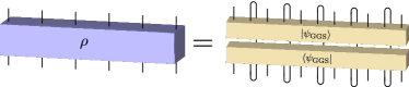
Figure 1: Graphical representation of a purification into a GGS. We restrict the discussion to mixed states that can be purified into GGSs, i.e., $\rho=\operatorname{Tr}_{A}[\ket{\psi_{\rm GGS}}\!\bra{\psi_{\rm GGS}}]$, for some GGS $\ket{\psi_{\rm GGS}}$ and subsystem $A$. We also require that $\rho$ has short-ranged Rényi-1 and -2 correlations, according to Definition 3. We refer to states that satisfy these properties as locally correlated mixed states.

The first condition generalizes the notion of short-range entangled (SRE) mixed states proposed in Ref. Ma:2022pvq (see also Ref. Ma:2023rji). Namely, a mixed state is SRE, if there is a purification into a SRE GGS. Here, we require that topologically ordered mixed states can be purified into GGSs more generally. The second condition rules out spontaneous symmetry breaking and long-range correlations, similar to the case for pure-state TOs.

The third condition is motivated by recent progress in understanding spontaneous symmetry breaking order in mixed states. In particular, it was found that observables that are nonlinear in the density matrix are necessary to characterize certain phases and phase transitions in mixed states Lee:2022hog; Bao:2023zry; Ma:2023rji. For example, the phenomenon known as strong-to-weak symmetry breaking can be detected by long-range order in the Rényi-2 correlations of local order parameters Lee:2022hog; Ma:2023rji.

We emphasize that this notion of locally-correlated mixed states allow us to give a working definition of TO. We do not claim that the conditions on mixed states above are the most exhaustive or the most general. Ultimately, one may want to consider a class of mixed states with no reference to Hamiltonians or replica Hilbert spaces. We comment further on this point in Section LABEL:sec:_discussion.

We note that a broader class of mixed states are those that can be decomposed into a convex sum of pure GGSs. All the examples of mixed states considered in this work can be represented as such a convex sum, but the converse is not true. The simplest counterexample is the thermal state of a classical Hamiltonian tuned to a finite-temperature critical point. Such a state contains purely classical long-range correlations and thus can not be purified into a GGS. Even assuming that correlation functions of local operators are all short-range, we can still find fully separable mixed states which do not admit a purification into a GGS Ma:2023rji.

An interesting question is whether a thermal state is locally correlated. Since a thermal state can always be purified into a thermofield double state, the question becomes whether the thermofield double state is the ground state of a gapped local Hamiltonian. To the best of our knowledge, the general case remains open, although Ref. Cottrell:2018ash proposed parent Hamiltonians for thermofield double states and presented evidence that the Hamiltonians are (quasi-)local. It was shown in Ref. Lucia:2021orn that thermofield double states for 2D Kitaev’s quantum double models are SRE. The same is true for thermal states of 1D local Hamiltonians.

II.2 Equivalence relation on mixed states

For ground states, a gapped phase is defined as an equivalence class of short-range correlated GGS, where the equivalence relation is given in terms of quasi-local unitary circuits (QLUCs), with at most $\rm polylog$ depth in the system size. Namely, two GGSs belong to the same phase if and only if they can be mapped to each other by a QLUC. Here, QLUC serves as a model for quasi-adiabatic evolution generated by a gapped local Hamiltonian.

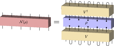
Figure 2: Graphical representation of a QLC $\mathcal{N}$. The action of the QLC $\mathcal{N}$ on a density matrix $\rho$ is equivalent to, in sequence, adding ancilla to $\rho$, conjugating by a QLUC $V$, and tracing out the ancilla (see Definition 4).

A natural generalization of QLUCs to mixed states is a quasi-local quantum channel (QLC), e.g., a finite time evolution generated by a local Lindbladian. However, because quantum channels are in general non-invertible, in order to define an equivalence relation, it becomes necessary to consider two-way connectedness by QLCs, which we take as the definition of mixed state phase Ma:2022pvq; Sang:2023rsp. Below, we first formalize the definition of a QLC (depicted in Fig. 2).

Definition 4.

A quantum channel $\mathcal{N}$ is a QLC if it can be purified into a circuit $V$, whose depth scales at most as $\mathrm{polylog}(L)$ with the linear system size $L$, acting on $\mathcal{H}\otimes\mathcal{H}_{A}$. Here, $\mathcal{H}$ and $\mathcal{H}_{A}$ are the physical and ancillary Hilbert spaces, respectively. The action of $\mathcal{N}$ on a mixed state $\rho$ is thus given by $\operatorname{Tr}[V^{\dagger}(\rho\otimes|0\rangle\langle 0|)V]$, where $|0\rangle$ represents a many-body product state in $\mathcal{H}_{A}$.

Following Refs. Ma:2022pvq; Ma:2023rji; Sang:2023rsp, we define mixed-state TOs using the following equivalence relation:

Definition 5.

Two locally-correlated mixed states $\rho_{1}$ and $\rho_{2}$ are equivalent, or belong to the same mixed-state TO, if and only if they are two-way connected by QLCs. Namely, there exists two QLCs $\mathcal{N}_{12}$ and $\mathcal{N}_{21}$ such that $\rho_{1}=\mathcal{N}_{12}(\rho_{2})$ and $\rho_{2}=\mathcal{N}_{21}(\rho_{1})$.

We point out that this definition is closely related to the one in Ref. Coser2019classificationof, which essentially amounts to replacing QLCs with fast evolution by local Lindbladians. That is, evolution for time that grows sub-linearly (e.g. polylog) with the system size.

It is natural to define the trivial phase as the unique equivalence class containing the product states. In all known examples, a trivial mixed state can be written as a convex sum of SRE states, however the converse is not necessarily true. According to this definition, the maximally mixed state also belongs to the trivial phase. It can be constructed from a product state by applying depolarizing noise and the product state can be constructed from it by tracing it out and tensoring with the product state. Similar to the ground state case, we are allowed to freely stack trivial states, as it adding unentangled ancilla is part of the definition of QLCs. We also note that all bosonic invertible GGSs, e.g., the $E_{8}$ state in (2+1)$d$, belong to the trivial mixed-state phase Ma:2022pvq. This in particular means that the chiral central charge is no longer a well-defined invariant for mixed state TOs.

We make two further comments:

1. Intuitively, one expects that thermal states of a local Hamiltonian at different positive temperature belong to the same mixed-state phase if there is no thermal phase transition in between. This has been proven in 1D. That is, all thermal states with positive temperature can be two-way connected by QLCs Kato:2016pgk.

2. A topological code with a small amount of noise, which can be modeled by applying a finite-depth quantum channel close to the identity to the pure state, is expected to belong to the same phase as the pure state. This has been demonstrated explicitly in the example of a $\mathbb{Z}_{2}$ TC with bit-flip noise in Sang:2023rsp (see also Sang:2024vkl and Bauer:2024qpc).

II.3 Locally indistinguishable states

A hallmark of TO for GGSs is that there is a topological degeneracy when the system is put on a torus – with the dimension of the ground state subspace being equal to the number of anyon types. The degeneracy for a higher-genus surface can also be determined from the anyon theory. Moreover, the ground states are locally indistinguishable, meaning that any two ground states $\ket{\psi_{1}}$ and $\ket{\psi_{2}}$ have the property

$$\braket{\psi_{1}}{M}{\psi_{1}}-\braket{\psi_{2}}{M}{\psi_{2}}=O(L^{-\infty}),$$ (6)

for any quasi-local operator $M$. Here, $L$ is the system size, and $O(L^{-\infty})$ is a function that decays faster than any power law of $L$, e.g. $e^{-(L/\xi)^{\alpha}}$ for any $\alpha>0$.

The notion of local indistinguishability naturally generalizes to mixed states. We say that two mixed states $\rho_{1}$ and $\rho_{2}$ are locally indistinguishable, if they satisfy Tr[M ρ_1] - Tr[Mρ_2 ] = O(L^-∞), for any quasi-local operator $M$.

In contrast to the pure-state case, the collection of locally indistinguishable mixed states do not form a vector space. Rather they form a convex manifold. As pointed out in Ref. Li:2024rgz, it is insightful to consider the extremal submanifold, i.e., the submanifold of extremal points. In general, this submanifold contains several connected components. Each connected component can have one of the following two possibilities:

1. It is a single point. In this case, the state is completely “classical”.

2. There is a continuum of extremal points forming a connected manifold of dimension $d$. Physically, this manifold should be isomorphic to the manifold of pure states in a $d$-dimensional Hilbert space. We refer to this space as a “coherent space” of dimension $d$. Note that an isolated extremal point can be thought of as a 0-dimensional coherent space.

We also note that two locally indistinguishable states $\rho_{1}$ and $\rho_{2}$ remain so under an arbitrary QLC. Explicitly, for an arbitrary QLC $\mathcal{N}$ and a quasi-local operator ${M}$, we can compute Tr[M N(ρ_1)] &= Tr[N^*(M) ρ_1 ],
= Tr[N^*(M) ρ_2 ],
= Tr[M N(ρ_2)], where $\mathcal{N}^{*}$ is the dual channel, which preserves quasi-locality. Therefore, the states $\mathcal{N}(\rho_{1})$ and $\mathcal{N}(\rho_{2})$ are also locally indistinguishable for any QLC $\mathcal{N}$.

However, the discussion above does not mean that the convex manifold of locally indistinguishable states must be invariant under QLCs, for two reasons. First, two locally distinguishable states may become indistinguishable under the QLC. This can happen, for example, if $\mathcal{N}^{*}(M)=0$ for all quasi-local operators $M$ that distinguished the two states. An example that illustrates this point is discussed in Section II.4. On the other hand, it can also happen that two different states that are locally indistinguishable become identical under a QLC. A simple example is a swap channel that takes any (pure state) TO to a trivial product state, under which the space of locally indistinguishable states is completely erased. In either case, the QLC is degenerate, i.e., it has a nontrivial kernel when viewed as a linear map on the space of operators.

In fact, the convex manifold of locally indistinguishable states is not an invariant for a mixed-state phase, as illustrated by the example in Section II.4. However, mixed-state TOs still give rise to coherent spaces of locally indistinguishable states on closed oriented manifolds, which depend on the topology of the manifold – similar to ground state TOs. We conjecture that there is a subspace within the coherent space that is robust to perturbations of the mixed state, and that this subspace provides an invariant for the mixed-state phase.

Lastly, one could consider the Rényi-2 (Rényi-$n$) expectation values to distinguish between states. It is possible that these higher-Rényi expectation values are able to distinguish between states that are otherwise locally indistinguishable according to the Rényi-1 expectation values. One can thus formulate different notions of local indistinguishability based on observables that are nonlinear in $\rho$, as recently proposed in Ref. Li:2024rgz. Although, we do not consider such notions of local indistinguishability any further in this work.

II.4 Example: decohered 2D toric code

To exemplify the general discussion above, we consider decohering a (2+1)$d$ TC state with bit-flip noise Dennis:2001nw; Fan:2023rvp. We recall that the TC state is defined on a square lattice with a qubit on each link, and with stabilizers given by

$$A_{v}=\prod_{v\in e}X_{e},\quad B_{p}=\prod_{e\in p}Z_{e}.$$ (7)

A ground state $\ket{\psi}$ is defined by $A_{v}\ket{\psi}=\ket{\psi},B_{p}\ket{\psi}=\ket{\psi}$ for all $v$ and $p$. The corresponding density matrix is denoted by $\rho_{0}=\ket{\psi}\!\bra{\psi}$. Following the common convention, we call a vertex violation $A_{v}=-1$ an $e$ particle at the vertex $v$, and a plaquette violation $B_{p}=-1$ an $m$ particle in the plaquette $p$.

Now, suppose that the TC is subjected to noise described by the bit-flip channel $\rho_{X}=\mathcal{N}_{X}(\rho_{0})$, defined as

$${\mathcal{N}}_{X}=\bigotimes_{e}{\mathcal{N}}_{X,e},\quad{\mathcal{N}}_{X,e}(\rho)=(1-p)\rho+pX_{e}\rho X_{e}.$$ (8)

Here, $p$ parameterizes the strength of the decoherence and satisfies $0\leq p\leq 1/2$. For small $p$, the TO still persists up to some critical value $p=p_{c}\approx 0.109$. For $p>p_{c}$, the system enters a new error-induced phase where the TO is lost. This transition can be characterized using quantum information-theoretic measures Fan:2023rvp. For example, for small $p$ we can view the TC as a quantum memory that encodes two logical qubits on a torus. For $p>p_{c}$, no coherent quantum information can be stored on a torus anymore. The same transition can be detected by topological entanglement negativity, which is $\ln 2$ before the transition and $0$ after Fan:2023rvp.

To understand the error-induced phase, it is particularly instructive to consider the strong-decoherence limit, i.e., $p=1/2$. There are a number of equivalent ways to represent the density matrix in this limit. If we work in the eigenbasis of the $X_{e}$ operators, and use the loop picture, where $X_{e}=-1$ means the link $e$ is occupied by a $\mathbb{Z}_{2}$ string, then the density matrix becomes a classical ensemble of $X$ loops:

$$\rho_{X}\propto\sum_{C}\ket{C}\!\bra{C}.$$ (9)

Here, $C$ denotes closed loops on the lattice.

One can think of this mixed state as a classical $\mathbb{Z}_{2}$ gauge theory and the $C$ as the electric field lines, defined by the Gauss law, or the closed loop condition. To some extent, the ensemble represents a classical TO Castelnovo2007: when put on a torus, there are four different ensembles distinguished by the winding number mod 2 of loops around the two non-contractible cycles. These four ensembles can not be distinguished by local observables, but they cannot form coherent superposition. Instead, one can form a classical mixture (i.e., a convex sum) of the classical states. In other words, the space of locally indistinguishable states consists of four isolated extremal points (see below for a more detailed discussion).

Another way to write the state is to directly expand the bit-flip channel:

$$\rho_{X}=\frac{1}{2^{N_{e}}}\sum_{n_{e}=0,1}\Big{(}\prod_{e}X_{e}^{n_{e}}\Big{)}\ket{\psi}\!\bra{\psi}\Big{(}\prod_{e}X_{e}^{n_{e}}\Big{)}.$$ (10)

Note that the state $\prod_{e}X_{e}^{n_{e}}\ket{\psi}$, in general, contains a number of $m$ particles. Fixing a particular configuration of $m$ particles, there are $2^{N_{v}-1}$ many ways to create it (the $-1$ is because $\prod_{v}A_{v}=1$ on a torus), so the state can also be written as

$$\rho_{X}=\frac{1}{2^{N_{e}-N_{v}+1}}\sum_{\mathbf{m}}\ket{\mathbf{m}}\!\bra{\mathbf{m}}.$$ (11)

Here, $\mathbf{m}$ denotes a configuration of $m$ anyons, with the constraint that, in total, there should be even number of them, and $\ket{\mathbf{m}}$ is the state with the corresponding configuration of $m$ anyons. Therefore, the density matrix describes an “incoherent” proliferation of $m$ particles. This should be contrasted with a “coherent” proliferation:

$$\ket{\psi_{m}}\propto\sum_{\mathbf{m}}\ket{\mathbf{m}}=\prod_{e}\frac{1+X_{e}}{2}\ket{\psi},$$ (12)

which is just a product state with $X_{e}=1$ everywhere.

A useful fact is that for $p>p_{c}$, the decohered TC state can be purified into a SRE state. This is most easily seen at $p=1/2$, where one can start from the product state $\ket{X_{e}=1}$, and apply the following quantum channel:

$$\mathcal{E}=\prod_{p}\mathcal{E}_{p},\quad\mathcal{E}_{p}=\frac{1}{2}(\rho+B_{p}\rho B_{p}).$$ (13)

Ref. Chen:2023vxo showed that the same is true for $p_{c}<p<1/2$. This allows one to show that the entire $p>p_{c}$ phase is trivial, in the sense defined in Section II.2. For $p=1/2$, we have already found a channel that maps a product state to a the decohered TC state. To show two-way connectedness, we just need to find a channel to map the decohered TC state to a product state. This can be done by simply tracing out the decohered state and appending a product state.

Finally, let us discuss some subtleties related to the space of locally indistinguishable states for the system defined on a sphere. For simplicity, let us focus on those states which are locally identical to the decohered TC ground state. We first notice that the full Hilbert space of the system on a sphere can be labeled by the eigenvalues of $A_{v}$ and $B_{p}$.

Let us now consider the subspace $\mathcal{H}_{m}$ of states that satisfy $A_{v}=1$, for every vertex $v$. In other words, $\mathcal{H}_{m}$ is the space of states with only $m$ anyon excitations. The most relevant local operator is $B_{p}$ here, which detects whether there is an $m$ anyon. The plaquette operators and the Pauli $X$ operators, in fact, generate all operators that keep the subspace $\mathcal{H}_{m}$ invariant. For a state $\ket{\psi}\in\mathcal{H}_{m}$, we have

$$\operatorname{Tr}\big{[}\mathcal{N}_{X}(\ket{\psi}\!\bra{\psi})B_{p}\big{]} =\operatorname{Tr}\big{[}\ket{\psi}\!\bra{\psi}\mathcal{N}_{X}(B_{p})\big{]}$$ (14)

$$=(1-2p)^{4}\braket{\psi}{B_{p}}{\psi}.$$ (15)

Curiously, if $p=1/2$, then the expectation value of $B_{p}$ is always 0 for any $\ket{\psi}\in\mathcal{H}_{m}$. Thus the dimension of locally indistinguishable states is $2^{N_{p}-1}$, where $N_{p}$ is the number of plaquettes. This is an example of the phenomenon mentioned earlier, i.e., that locally distinguishable states can become indistinguishable under a QLC.

However, if $p\neq 1/2$, clearly the result is very different. For example, if $\ket{\psi}$ contains $m$ anyons at fixed locations, $\mathcal{N}(\ket{\psi}\!\bra{\psi})$ is still locally distinguishable from the decohered ground state. Thus, identifying locally indistinguishable states amounts to finding states in the subspace $\mathcal{H}_{m}$ such that the expectation value of $B_{p}$ is sufficiently close to $1$. One example is to consider a state $\ket{p_{1},p_{2}}$ with a pair of ${m}$ anyons, say at plaquettes $p_{1},p_{2}$, and then superpose all such states with two ${m}$ anyons:

$$\ket{\Psi}=\sqrt{\frac{2}{N_{p}(N_{p}-1)}}\sum_{p_{1}\neq p_{2}}\ket{p_{1},p_{2}}.$$ (16)

We find that $\braket{\Psi}{B_{p}}{\Psi}=1-O(L^{-2})$. However, this does not meet the criterion for local indistinguishability in Eq. (II.3), as we require that the correction should decay super-polynomially in $L$. In fact, this is the generic situation: in order for $\braket{B_{p}}$ to be close to 1, the density of $m$ anyons must be 0. In other words, there are $O(1)$ such anyons. Suppose the typical number of $m$ anyons is $n$. To get a uniform state one has to superpose states with different configurations, so the weight of a state with a definition configuration is on average $O(L^{-n})$. Then the expectation value $\braket{B_{p}}$ is $1-O(L^{-2})$, which does not satisfy the criterion for local indistinguishability. We thus find that the space of locally indistinguishable states on a sphere consists of just a single classical state.

Now, we move on to consider locally indistinguishable states on a torus for $p$ slightly below $1/2$, to avoid the kind of exponentially large number of states created by populating $m$ anyon excitations. This is strong evidence that the mixed state belongs to the trivial phase. On the other hand, we also know that for $p_{c}<p<1/2$ the manifold of locally indistinguishable states has four extremal points, labeled by the eigenvalues of the non-contractible Wilson loops of $m$ anyons. This is different from a product state, but does not preclude the decohered state from having trivial mixed-state TO.

III Decohered Pauli stabilizer states

In this section we study general topological stabilizer states, under Pauli decoherence channels. More explicitly, we consider a Pauli stabilizer state $\ket{\psi}$ defined by the Pauli stabilizer group ${\mathcal{S}}_{0}$. Namely, $\ket{\psi}$ satisfies

$$S\ket{\psi}=\ket{\psi},\,\,\forall S\in{\mathcal{S}}_{0}.$$ (17)

We assume that ${\mathcal{S}}_{0}$ admits a set of local generators and that, on an infinite plane, the only Pauli operators that commute with every element of $\mathcal{S}_{0}$ are the elements of $\mathcal{S}_{0}$. These are the conditions for a stabilizer code to be topological Haah2021classification.

Then, suppose that we apply a QLC ${\mathcal{N}}$ of the form:

$${\mathcal{N}}=\prod_{i}{\mathcal{N}}_{i},\quad\>{\mathcal{N}}_{i}(\rho)=\sum_{r=1}^{n}p_{r}P_{i,r}\rho P^{\dagger}_{i,r}.$$ (18)

where $P_{i,r}$ is a local Pauli operator, and $p_{1},p_{2},\dots,p_{n}$ satisfy $p_{r}\geq 0$ and $\sum_{r=1}^{n}p_{r}=1$. Here, we assume the channel is translation-invariant. Note that while the $P_{i,r}$ operators do not always commute, they are all Pauli operators, so the commutator between any two of them is always a phase factor. Therefore, the channels actually commute:

$${\mathcal{N}}_{i}\circ{\mathcal{N}}_{j}={\mathcal{N}}_{j}\circ{\mathcal{N}}_{i}.$$ (19)

Denote by ${\mathcal{G}}$ the algebra of local operators generated by the $P_{i,r}$’s and ${\mathcal{S}}_{0}$. In order to analyze the effect of the quantum channel, it turns out to be convenient to think of the problem as a subsystem code, which we now briefly review.

III.1 Topological subsystem codes

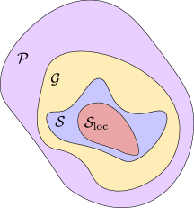
Figure 3: Containment of the groups for defining a topological subsystem code. The gauge group $\mathcal{G}$ (yellow) is an arbitrary subgroup of the Pauli group $\mathcal{P}$ (purple). The stabilizer group $\mathcal{S}$ (blue) is the center of $\mathcal{G}$ up to roots of unity. Finally, the subgroup of locally generated stabilizers $\mathcal{S}_{\rm loc}$ (red) is contained in $\mathcal{S}$. If the subsystem code is topological, then $G$ admits a set of local generators, and on an infinite plane, there are no logical operators and $\mathcal{S}_{\rm loc}=\mathcal{S}$.

Let us briefly review the theory of Pauli subsystem codes PoulinPRL2005; BombinPRB2009; BombinTSC; Ellison:2022web. The starting point is the “gauge group” ${\mathcal{G}}$, which is a group of Pauli operators. The elements of ${\mathcal{G}}$ are referred to as gauge operators. We then define the stabilizer group ${\mathcal{S}}$ of the subsystem code as the center of ${\mathcal{G}}$:

$${\mathcal{S}}\propto{\mathcal{Z}}({\mathcal{G}}).$$ (20)

Here, the proportionality symbol means that ${\mathcal{S}}$ is defined up to roots of unity. We return to this issue later. The stabilizer group defines the code space ${\mathcal{H}}_{C}$:

$${\mathcal{H}}_{C}=\{\ket{\psi}:S\ket{\psi}=\ket{\psi},\forall S\in{\mathcal{S}}\}.$$ (21)

By Eq. (20), the gauge operators preserve the code space. We show the containment of the various groups of Pauli operators in Fig. 3.

Unlike ordinary stabilizer codes, in a subsystem code, quantum information is only stored in a subsystem of ${\mathcal{H}}_{C}$, known as the logical subsystem. More precisely, with ${\mathcal{G}}$ and ${\mathcal{S}}$, we have the following decomposition of the Hilbert space:

$${\mathcal{H}}={\mathcal{H}}_{C}\oplus{\mathcal{H}}_{C}^{\perp},\quad\>{\mathcal{H}}_{C}={\mathcal{H}}_{G}\otimes{\mathcal{H}}_{L}.$$ (22)

Here, ${\mathcal{H}}_{G}$ is the gauge system, such that ${\mathcal{G}}/{\mathcal{S}}$ acts on ${\mathcal{H}}_{G}$ faithfully and irreducibly as the Pauli algebra. ${\mathcal{H}}_{L}$ is the logical subspace, on which the gauge operators act as the identity. When ${\mathcal{G}}$ is proportional to ${\mathcal{S}}$, the gauge subsystem ${\mathcal{H}}_{G}$ is trivial and the subsystem code is equivalent to a stabilizer code defined by ${\mathcal{S}}$. Similar to stabilizer codes, a logical operator is a Pauli operator that preserves the code space. All logical operators form the group ${\mathcal{Z}}_{\mathcal{P}}({\mathcal{S}})$, which is the centralizer of ${\mathcal{S}}$ in the Pauli group ${\mathcal{P}}$, i.e., the subgroup of Pauli operators that commute with every element of $\mathcal{S}$. A nontrivial logical operator should act nontrivially on ${\mathcal{H}}_{L}$; this is given by the group ${\mathcal{Z}}_{\mathcal{P}}({\mathcal{S}})/{\mathcal{G}}$

So far, our definition of subsystem codes is for a generic quantum system without any notion of locality. For a local quantum system, we further require that ${\mathcal{G}}$ is generated by local Pauli operators. Notice that this does not have to be true for ${\mathcal{S}}$: it may contain nonlocal generators. For simplicity, we also assume that ${\mathcal{G}}$ is translation invariant.

A subsystem code is topological if (1) $\mathcal{G}$ admits a set of local generators, and (2) on an infinite plane, there are no logical operators and ${\mathcal{S}}$ can be generated by local operators. We primarily consider topological subsystem codes in the discussion below.

In order to study the decohered stabilizer code on torus (or higher-genus surfaces), it is useful to introduce further structure, since the stabilizer group ${\mathcal{S}}$ may contain nonlocal generators. We therefore split ${\mathcal{S}}$ into a locally-generated subgroup ${\mathcal{S}}_{\rm loc}$ and ${\mathcal{S}}_{T}$, such that ${\mathcal{S}}/{\mathcal{S}}_{\rm loc}={\mathcal{S}}_{T}$. Here, the subgroup ${\mathcal{S}}_{\rm loc}$ is generated by geometrically local stabilizers. We define a “local” code space according to ${\mathcal{S}}_{\rm loc}$:

$${\mathcal{H}}={\mathcal{H}}_{lC}\oplus{\mathcal{H}}_{lC}^{\perp}.$$ (23)

Namely, ${\mathcal{H}}_{lC}$ is the subspace with $S=1$ for every $S\in{\mathcal{S}}_{\rm loc}$.

Then, we further split ${\mathcal{H}}_{lC}$ according to eigenvalues of ${\mathcal{S}}_{T}$. Denote by ${t}$ a group homomorphism from ${\mathcal{S}}_{T}$ to $\mathrm{U}(1)$, such that $t(T)$ is an eigenvalue of $T$. Indexing the generators of $\mathcal{S}_{T}$ by $i$, we can define a vector $\mathbf{t}$ whose $i$th entry is $\mathbf{t}_{i}=t(T_{i})$. With this, $\mathcal{H}_{lC}$ decomposes as

$${\mathcal{H}}_{lC}=\bigoplus_{\mathbf{t}}{\mathcal{H}}_{lC}^{\mathbf{t}},$$ (24)

where the subspace ${\mathcal{H}}_{lC}^{\mathbf{t}}$ is labeled by a vector $\mathbf{t}$. Every state in ${\mathcal{H}}_{lC}^{\mathbf{t}}$ is an eigenstate of $T\in{\mathcal{S}}_{T}$ with eigenvalue $\mathbf{t}_{i}=t(T)$. We take ${\mathcal{H}}_{lC}^{\mathbf{t}=\mathbf{1}}$ to be the code space ${\mathcal{H}}_{C}$. Each ${\mathcal{H}}_{lC}^{\mathbf{t}}$ can be further factorized as

$${\mathcal{H}}_{lC}^{\mathbf{t}}={\mathcal{H}}_{G}^{\mathbf{t}}\otimes{\mathcal{H}}_{L}^{\mathbf{t}}.$$ (25)

For each $\mathbf{t}$ subspace, we can define a stabilizer group ${\mathcal{S}}^{\mathbf{t}}$, which is generated by ${\mathcal{S}}_{\rm loc}$ and $t(T_{i})^{-1}T_{i}$.

III.2 Decohered topological stabilizer states

Now, we return to the decohered stabilizer code. The initial (local) stabilizer group of the code is ${\mathcal{S}}_{0}$. The Pauli errors $P_{i,r}$ generate a group $E$. It is natural to assume that any element $e$ of $E$ at least fails to commute with some stabilizer in ${\mathcal{S}}_{0}$, otherwise, by the assumption of ${\mathcal{S}}_{0}$ being topological, $e$ must belong to ${\mathcal{S}}_{0}$ as well.

We consider the subsystem code defined by the gauge group ${\mathcal{G}}=\braket{{\mathcal{S}}_{0},E}$. We assume that the subsystem code defined by this gauge group is topological. We emphasize that this is a nontrivial condition. Indeed in Section III.4.3, we discuss an example where this condition is not met. We note that, in particular, the topological condition guarantees that the decohered stabilizer state is locally correlated. First of all, the decohered state admits a purification into a GGS, since it is constructed by adding Pauli noise to a topological stabilizer state. Furthermore, we show in Appendix LABEL:app:_Renyi2_topological_codes that it is Rényi-1 and -2 locally correlated.

We now consider the maximum decoherence limit and argue that the topological stabilizer state becomes maximally mixed on the subsystem ${\mathcal{H}}_{G}^{\mathbf{t}}$. In agreement with the the subsystem code literature, the subsystem ${\mathcal{H}}_{L}^{\mathbf{t}}$ defines a noiseless subsystem Knill2000noiseless; Kribs2006operator.

We first observe that, for a state $\rho_{0}$ in the code space of ${\mathcal{S}}_{0}$, we can write

$${\mathcal{N}}(\rho_{0})=\sum_{g\in{\mathcal{G}}}p_{g}g\rho g^{\dagger},$$ (26)

where the sum is over all elements of the gauge group ${\mathcal{G}}$. Unlike Eq. (18), the expression for the action of $\mathcal{N}$ on $\rho_{0}$ includes the stabilizers of $\mathcal{S}_{0}$. Since $\rho_{0}$ is invariant under the elements of $\mathcal{S}_{0}$, this just adds an overall constant factor, which is absorbed into the normalization. The maximal decoherence limit then corresponds to taking $p_{g}=\frac{1}{|{\mathcal{G}}|}$. We denote the channel in this limit by ${\mathcal{N}}_{m}$. As we saw in the $\mathbb{Z}_{2}$ TC example, the physics of the error-induced phase is well captured by this limit.

We would now like to argue that $\mathcal{N}_{m}$ acting on an arbitrary pure state $\rho_{0}=\ket{\psi}\!\bra{\psi}$ in the code space of $\mathcal{S}_{0}$ creates a maximally-mixed state in the gauge subsystem. That is, we would like to show that N_m(ρ_0) = ∑_t1dimHGt1_H_G^t⊗ρ_L^t, for some state $\rho_{L}^{\mathbf{t}}$ on the logical subsystem. This follows immediately from the fact that the gauge group generates the full matrix algebra on the gauge subsystem Knill2000noiseless; Zanardi2004Tensor; Kribs2006operator. Therefore, the channel in Eq. (26) behaves like the depolarizing noise channel within the gauge subsystem. Nonetheless, we find it instructive to demonstrate Eq. (III.2) explicitly.

We begin by noticing that the state $\rho_{0}=\ket{\psi}\!\bra{\psi}$ belongs to the code space $\mathcal{H}_{lC}$, since ${\mathcal{S}}_{\rm loc}\subset{\mathcal{S}}_{0}$. According to Eq. (24), this means that we can decompose $\ket{\psi}$ as

$$\ket{\psi}=\sum_{\mathbf{t}}\ket{\psi^{\mathbf{t}}},\quad\ket{\psi^{\mathbf{t}}}\in\mathcal{H}_{lC}^{\mathbf{t}},$$ (27)

where $\ket{\psi^{\mathbf{t}}}$ is

$$\ket{\psi^{\mathbf{t}}}=\frac{1}{|\mathcal{S}_{T}|}\sum_{T\in{\mathcal{S}}_{T}}t(T)^{-1}T\ket{\psi}.$$ (28)

Given the factorization of the code space, we can further Schmidt decompose $\ket{\psi_{\mathbf{t}}}$ to obtain

$$\ket{\psi^{\mathbf{t}}}=\sum_{\alpha}\lambda_{\mathbf{t},\alpha}\ket{\psi^{\mathbf{t}}_{G,\alpha}}\otimes\ket{\psi^{\mathbf{t}}_{L,\alpha}}.$$ (29)

Here, the states $\ket{\psi^{\mathbf{t}}_{G/L,\alpha}}$ are orthonormal for different indices $\alpha$, and ${\sum_{\alpha}\lambda_{\mathbf{t},\alpha}^{2}=1}$.

With this notation, the action of $\mathcal{N}_{m}$ on $\rho_{0}$ can be written as

$${\mathcal{N}}_{m}(\rho_{0})=\\ \sum_{\mathbf{t},\mathbf{t}^{\prime}}\sum_{\alpha,\beta}\lambda_{\mathbf{t}\alpha}^{*}\lambda_{\mathbf{t}^{\prime}\beta}{\mathcal{N}}_{m}(\ket{\psi_{G,\alpha}^{\mathbf{t}}}\!\bra{\psi_{G,\beta}^{\mathbf{t}^{\prime}}})\otimes\ket{\psi_{L,\alpha}^{\mathbf{t}}}\!\bra{\psi_{L,\beta}^{\mathbf{t}^{\prime}}}.$$ (30)

We have used here that, by definition, the gauge operators act as the identity on the logical subsystem. We see that, to understand the effects of the channel $\mathcal{N}_{m}$, we only need to consider its effects on $\ket{\psi_{G,\alpha}^{\mathbf{t}}}\!\bra{\psi_{G,\beta}^{\mathbf{t}^{\prime}}}$.

By explicit calculation, we find that $\mathcal{N}_{m}(\ket{\psi_{G,\alpha}^{\mathbf{t}}}\!\bra{\psi_{G,\beta}^{\mathbf{t}^{\prime}}})$ is

$${\mathcal{N}}_{m}(\ket{\psi^{\mathbf{t}}_{G,\alpha}}\!\bra{\psi^{\mathbf{t}^{\prime}}_{G,\beta}})=\frac{1}{|\mathcal{G}|}\sum_{g\in{\mathcal{G}}}g\ket{\psi^{\mathbf{t}}_{G,\alpha}}\!\bra{\psi^{\mathbf{t}^{\prime}}_{G,\beta}}g^{\dagger}\\ =\sum_{\tilde{g}\in{\mathcal{G}}/{\mathcal{S}}_{T}}\tilde{g}\ket{\psi^{\mathbf{t}}_{G,\alpha}}\!\bra{\psi^{\mathbf{t}^{\prime}}_{G,\beta}}\tilde{g}^{\dagger}\sum_{T\in{\mathcal{S}}_{T}}t(T){t^{\prime}}(T)^{-1}.$$ (31)

To obtain the second line, we split the gauge operator $g$ into $g=\tilde{g}T$, and used $T\ket{\psi_{G}^{\mathbf{t}}}=t(T)\ket{\psi_{G}^{\mathbf{t}}}$. Next, we use the following identity:

$$\sum_{T\in{\mathcal{S}}_{T}}t(T){t^{\prime}}(T)^{-1}=|{\mathcal{S}}_{T}|\delta_{\mathbf{t},\mathbf{t}^{\prime}}.$$ (32)

This allows us to write N_m(|ψ^t_G, α⟩​⟨ψ^t’_G,β|) = |ST||G|δ_t,t’∑_~g∈G/S_T~g|ψ^t_G,α⟩​⟨ψ^t’_G,β|~g^†.

Now, we only need to prove that

$${\mathcal{N}}_{m}(\ket{\psi_{G,\alpha}^{\mathbf{t}}}\!\bra{\psi_{G,\beta}^{\mathbf{t}}})=\delta_{\alpha\beta}\frac{1}{\dim{\mathcal{H}}_{G}^{\mathbf{t}}}\mathds{1}_{{\mathcal{H}}_{G}^{\mathbf{t}}}.$$ (33)

We prove this for $\mathbf{t}=\mathbf{1}$. For other $\mathbf{t}$, we can just replace ${\mathcal{S}}$ with ${\mathcal{S}}^{\mathbf{t}}$. For brevity, we drop the $\mathbf{t}$ superscript. For any Pauli operator $O$ in the gauge subsystem, we have

$$\begin{split}{\mathcal{N}}_{m}(O)=\frac{1}{|{\mathcal{G}}/{\mathcal{S}}|}\sum_{\tilde{g}\in{\mathcal{G}}/{\mathcal{S}}}\tilde{g}O\tilde{g}^{\dagger}=\begin{cases}O,&\text{if }O\propto\mathds{1}\\ 0,&{\rm otherwise}.\end{cases}\end{split}$$ (34)

This follows from the fact that ${\mathcal{G}}/{\mathcal{S}}$ is isomorphic to the Pauli algebra on the gauge subsystem. Then, for a general operator $O$ in the gauge subsystem, it follows that

$${\mathcal{N}}_{m}(O)=\operatorname{Tr}O\cdot\frac{1}{\dim{\mathcal{H}}_{G}}\mathds{1}.$$ (35)

Given that $\operatorname{Tr}(\ket{\psi_{G,\alpha}^{\mathbf{t}}}\!\bra{\psi_{G,\beta}^{\mathbf{t}}})=\delta_{\alpha\beta}$, we arrive at Eq. (33).

Putting this all together, we finally find that the maximally decohered state $\rho_{m}$ is

$${\mathcal{N}}_{m}(\rho_{0}) =\sum_{\mathbf{t}}\frac{1}{\dim{\mathcal{H}}_{G}^{\mathbf{t}}}\mathds{1}_{{\mathcal{H}}_{G}^{\mathbf{t}}}\otimes\sum_{\alpha}\lambda_{\mathbf{t},\alpha}^{2}\ket{\psi_{L,\alpha}^{\mathbf{t}}}\!\bra{\psi_{L,\alpha}^{\mathbf{t}}}$$

$$=\sum_{\mathbf{t}}\frac{1}{\dim{\mathcal{H}}_{G}^{\mathbf{t}}}\mathds{1}_{{\mathcal{H}}_{G}^{\mathbf{t}}}\otimes\rho_{L}^{\mathbf{t}}.$$

Physically, we have shown that after the maximal noise channel, the gauge subsystems are left in the maximally mixed state, but the state in the logical space ${\mathcal{H}}_{L}^{\mathbf{t}}$ is unaffected. Furthermore, there is no quantum coherence between logical subspaces with different $\mathbf{t}$: one can only form convex sum of $\rho_{L}^{\mathbf{t}}$’s. In a sense, ${\mathcal{S}}_{T}$ encodes classical information. Therefore, coherent spaces are labeled by the eigenvalues $\mathbf{t}$.

We remark that when the logical subsystem is trivial (e.g., when the model is placed on a sphere), the gauge subsystem is the code space, and we simply find a maximally mixed state in the code space. The density matrix can then be written as a stabilizer state fattal2004entanglement:

$$\rho_{m}=\frac{1}{|{\mathcal{S}}|}\sum_{S\in{\mathcal{S}}}S.$$ (36)

III.3 Abelian anyon theories

To identify interesting examples of decohered topological stabilizer states, beyond the decohered TC state in Section II.4, we find it valuable to introduce the language of anyon theories. In general, topologically ordered states in (2+1)$d$ are characterized by anyon theories, which are defined by abstract mathematical data consisting of a set of anyon types, their fusion rules, $F$-symbols, and $R$-symbols. For topological Pauli stabilizer states, however, the anyon theories are Abelian, meaning that the data simplifies greatly. To specify an Abelian anyon theory we need (1) an Abelian group $\mathcal{A}$ of anyons whose product represents the fusion of anyons, and (2) a function $\theta:\mathcal{A}\to\mathrm{U}(1)$ that determines the exchange statistics of the anyons. We note that a formal definition of anyon types for topological Pauli subsystem codes is given in Ref. Ellison:2022web.

The exchange statistics of the anyons can be determined by first identifying the string operators that move the anyons around the system, using, for example, the construction in Refs. Ellison:2022web; BombinPoulin2012Universal. The string operators can then be used to compute the exchange statistics following Refs. Levin2003fermion; Kawagoe2020; Ellison:2022web. The identity element $1\in\mathcal{A}$, is a boson, so it satisfies $\theta(1)=1$. Furthermore, $\theta(a)$ gives a quadratic form over the anyon group. This is to say that $\theta(na)=\theta(a)^{n^{2}}$, for any anyon type $a$. The $T$ matrix of the anyon theory is defined as T_ab = θ(a) δ_ab, for $a,b\in\mathcal{A}$.

Using $\theta$, we can also define a bilinear form $B(a,b)$ over ${\mathcal{A}}$, which captures the braiding relations between anyon types $a$ and $b$:

$$B(a,b)=\frac{\theta(ab)}{\theta(a)\theta(b)}.$$ (37)

An anyon theory is called “modular” if, for every anyon type $a$, there exists an anyon type $b$ such that $B(a,b)\neq 1$. Otherwise, the anyon theory is premodular (or non-modular). The $S$ matrix of the anyon theory is defined as

$$S_{ab}=\frac{1}{\sqrt{|\mathcal{A}|}}B(a,b).$$ (38)

If the anyon theory is modular, then the $S$ matrix is unitary. It is proven in Ref. Ellison:2022web that the anyon theory of a Pauli topological state is always modular. For Pauli topological subsystem codes, on the other hand, the anyon theory may be premodular.

If an anyon theory is premodular, then there exists at least one “transparent” anyon type $a$, such that $B(a,b)=1$, for every anyon type $b\in\mathcal{A}$. The subgroup of transparent anyons ${\mathcal{T}}$ is defined as

$${\mathcal{T}}=\{a\in{\mathcal{A}}\,|\,B(a,b)=1,\,\forall b\in{\mathcal{A}}\}.$$ (39)

For a modular theory, ${\mathcal{T}}$ consists of only the trivial anyon. In general, transparent anyons can be either bosons or fermions. We define $\mathcal{T}_{b}$ as the subgroup of the transparent anyons that have bosonic statistics.

One can form the quotient group $\mathcal{A}^{\rm{min}}={\mathcal{A}}/{\mathcal{T}}_{b}$. This defines another anyon theory, which can be interpreted as the anyon theory obtained from condensing the bosons in $\mathcal{T}$. If $\mathcal{T}=\mathcal{T}_{b}$, then, $\mathcal{A}^{\rm{min}}$ is modular. More generally, for Abelian anyon theories, $\mathcal{A}^{\rm min}$ takes the form $\mathcal{A}^{\rm min}=\mathcal{C}\boxtimes\mathbb{Z}_{2}^{(1)}$, where $\mathcal{C}$ is modular, $\boxtimes$ denotes the operation of stacking two independent anyon theories, and $\mathbb{Z}_{2}^{(1)}$ is the anyon theory generated by an order 2 transparent fermion (defined below).

To make the discussion more explicit, let us introduce a family of Abelian premodular anyon theories with a single generator. These anyon theories appear in the examples in the next section. Following Bonderson2012, the anyon theories are denoted by $\mathbb{Z}_{N}^{(p)}$, where $\mathbb{Z}_{N}$ indicates the fusion group, and $p$ is an integer for odd $N$ and a half-integer when $N$ is even. The group elements are denoted by $[a]$ with $a=0,1,\cdots,N-1$ defined mod $N$. The basic data is given by

$$[a]\times[b]=[a+b]$$ (40)

$$\theta([a])=e^{\frac{2\pi ip}{N}a^{2}},$$ (41)

$$B([a],[b])=e^{\frac{4\pi ip}{N}ab},$$ (42)

where addition is taken mod $N$. Intuitively, when $p$ is an integer, $\mathbb{Z}_{N}^{(p)}$ is the anyon theory generated by $em^{p}$ in a $\mathbb{Z}_{N}$ TC.

The transparent subgroup $\mathcal{T}$ can be determined from the data above. Here, we list a few common cases:

1. If $N$ is odd and $p\in\mathbb{Z}$, then the transparent subgroup is $\mathbb{Z}_{(p,N)}^{(0)}$. In particular, if $p$ is coprime with $N$ the theory is modular.

2. If $N$ is even and $p\in\mathbb{Z}$, the transparent subgroup is $\mathbb{Z}_{2(N/2,p)}$ generated by $[\frac{N/2}{(N/2,p)}]$. These theories are always non-modular.

3. If $N$ is even and $p\in\mathbb{Z}+\frac{1}{2}$, then the transparent subgroup $\mathbb{Z}_{(N,2p)}^{(0)}$ is generated by $[\frac{N}{(N,2p)}]$.

Let us now comment on the connection between anyon theories and the discussion of topological subsystem codes in the previous sections. As shown in Ref. Ellison:2022web, the nonlocal stabilizers ${\mathcal{S}}_{T}$ on a torus (or any higher-genus surface) are generated by the string operators of the transparent anyons ${\mathcal{T}}$ along non-contractible cycles. Once the values of ${\mathcal{S}}_{T}$ are fixed, the logical operators for the quantum coherent subspace ${\mathcal{H}}_{L}^{\mathbf{t}}$ are string operators of the modular part of $\mathcal{A}^{\rm{min}}$ along non-contractible cycles.

Let us also revisit the locally indistinguishable states of the decohered topological stabilizer codes, using the language of Abelian anyon theories. We consider the case when the system is put on a torus. Before adding noise, a basis for the ground state space can be chosen to be $\ket{a}_{x}$ where $a$ is the anyon label, and $\ket{a}_{x}$ is the eigenstate of Wilson loops around the $y$ direction of the torus. That is, for an arbitrary $a$, the state $\ket{a}_{x}$ satisfies

$$W_{y}(b)\ket{a}_{x}=\frac{S_{ab}}{S_{Ia}}\ket{a}_{x},\quad W_{x}(b)\ket{a}=\ket{a\times b}_{x}.$$ (43)

The coherent subspaces are eigenspaces of $W_{x}(t)$ and $W_{y}(t)$ for all $t\in\mathcal{T}$. Let us consider the $W_{x}(t)=W_{y}(t)=1$ subspace. This coherent subspace, in particular, can be obtained by decohering the following ground state subspace on a torus:

$$\text{span}\Big{\{}\frac{1}{\sqrt{|\mathcal{T}|}}\sum_{t\in\mathcal{T}}\ket{a\times t}_{x}\>\big{|}\>a\in\mathcal{A}\Big{\}}.$$ (44)

The basis states of the coherent space are in one-to-one correspondence with elements of $\mathcal{A}/\mathcal{T}$. Thus, the dimension of the coherent space is equal to $|\mathcal{A}/\mathcal{T}|$. When $\mathcal{T}=\mathcal{T}_{b}$, within the coherent space, the action of string operators for $\tilde{a}\in\mathcal{A}^{\rm min}$ that wrap around the torus is identical to that of a pure state TO with $\mathcal{A}^{\rm min}$ as the anyon theory.

III.4 Examples

III.4.1 $\mathbb{Z}_{2}$ toric code with $X$ noise

The first example is again the $\mathbb{Z}_{2}$ TC under bit-flip errors. Here, the stabilizer group ${\mathcal{S}}_{0}$ is generated by the vertex $A_{v}$ and plaquette $B_{p}$ stabilizers of the TC. The gauge group defined with bit-flip noise is ${\mathcal{G}}=\langle{\mathcal{S}}_{0},X\rangle$. The group ${\mathcal{S}}_{\rm loc}$ is generated by the $A_{v}$ and Pauli $X$ operators. The group ${\mathcal{S}}_{T}$ is then generated by the string operators of $X$ along non-contractible loops on the dual lattice. Physically, ${\mathcal{S}}$ are the closed string operators of the $m$ anyon. Therefore the associated Abelian anyon theory is ${\mathcal{A}}=\{1,m\}$, also known as $\mathbb{Z}_{2}^{(0)}$. The anyon theory consists only of transparent anyons (i.e., ${\mathcal{T}}={\mathcal{A}}$).

We have shown in Section II.4 that, in the maximal decoherence limit, the density matrix becomes a diagonal classical ensemble of closed loops. On a torus, the mod 2 winding numbers of the loops around two directions are topological invariants. Thus, we have four classical states:

$$\rho_{X}^{w_{x}w_{y}}\propto\sum_{C\in\mathbf{C}_{w_{x}w_{y}}}\ket{C}\!\bra{C},\quad\>w_{x/y}=0,1.$$ (45)

Here, $w_{x/y}$ indicates the even/odd parity of the number of loops wrapping around $x$ or $y$ directions, and $\mathbf{C}_{w_{x}w_{y}}$ is the corresponding set of loop configurations. These four states are precisely distinguished by the eigenvalues of the nonlocal stabilizers. A general density matrix is a convex sum of the four density matrices. In other words, there are four isolated extremal points in the space of locally indistinguishable states on a torus. The $e$ string operator of the TC, namely product of $Z$ operators along a path on the lattice, can toggle between the four extremal points.

III.4.2 $\mathbb{Z}_{2}$ toric code with “fermionic” noise

As described in Section II.4, bit-flip noise applied to the TC state can be interpreted as incoherently proliferating $m$ anyons. Here, we consider instead an incoherent proliferation of $f=e\times m$ particles. Note that since $f$ is a fermion, it can not be condensed coherently. However, an incoherent proliferation is still possible.

Since the fermion is a bound state of $e$ and $m$, one has to specify the relative positions. It is useful to fix an orientation, where the $m$ is always at the plaquette $p$ to the “northeast” of $e$ at the vertex $v$. We say that such a bound state is a fermion at the plaquette $p$.

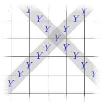
(a)

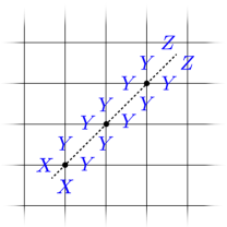
(b)

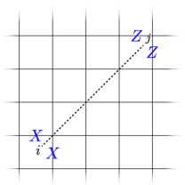
(c)

Figure 4: The $Y$-decohered TC state and its Rényi-2 order parameters. (a) The stabilizer group of the $Y$-decohered TC subsystem code is generated by products of Pauli $Y$ operators along diagonals. (b) A product of $A_{v}B_{\rm{NE}(v)}$ operators along a diagonal path (dashed line) yields $XX$ operators at one endpoint and $ZZ$ operators at the other, separated by a string of $Y$ operators. (c) The Rényi-2 correlator $C^{(2)}\big{(}(XX)_{i},(ZZ)_{j}\big{)}$ exhibits long-range correlations for $i$ and $j$ along a diagonal.

We can then define a “hopping” operator $S_{e}$ for each link $e$.

$$S_{e}=\vbox{\hbox{\includegraphics[scale={0.21}]{Figures/z2emh2.pdf}}},\,\,\quad\vbox{\hbox{\includegraphics[scale={0.21}]{Figures/z2emv2.pdf}}}.$$ (46)

The hopping operator $S_{e}$ creates, annihilates, or moves the fermions between the plaquettes bordered by the edge $e$. We consider the following channel, which incoherently proliferates the fermions:

$${\mathcal{N}}_{f}=\prod_{e}{\mathcal{N}}_{f,e},\quad{\mathcal{N}}_{f,e}(\rho)=\frac{1}{2}(\rho+S_{e}\rho S_{e}).$$ (47)

For a TC state $\rho_{0}$, we define $\rho_{f}={\mathcal{N}}_{f}(\rho_{0})$. We refer to this state as the fermion-decohered TC state.

To better understand the decohered state, we employ the fermionization map introduced in Chen:2017fvr. This map takes the subspace satisfying $A_{v}B_{\rm{NE}(v)}=1$, where $\rm{NE}(v)$ is the plaquette to the northeast of the vertex $v$, to the fermion parity even sector of a system with physical fermions on the plaquettes. The initial TC ground state has no $f$ excitations. After the channel is applied, one can show that the density matrix in the fermionic Hilbert space takes the following form:

$$\rho_{f}=\frac{1}{2^{N_{p}-1}}{\sum_{\{n_{p}\}}}^{\prime}\ket{\{n_{p}\}}\!\bra{\{n_{p}\}}\propto 1+P_{f},$$ (48)

where $n_{p}$ denotes the fermion occupancy at the plaquette $p$, and the sum is over configurations $\{n_{p}\}$ satisfying $\sum_{p}n_{p}=0\text{ mod }2$. This gives the maximally mixed state in the ${P_{f}=1}$ subspace . After bosonization, the fermionic density matrix $\rho_{f}$ is again mapped to the fermion-decohered TC state (hence the same notation).

Interestingly, we find that $\rho_{f}$ has many other purifications. For example, it can be purified into an Ising TO, or any of the Kitaev’s 16-fold ways Kitaev:2005hzj. This is elaborated on in Appendix LABEL:app:purify-fermion-TC.

One can show that $\rho_{f}$ is not SRE in a bosonic system, but can have a SRE purification, if there are physical fermions in the system. It was recently suggested in Ref. Wang:2023uoj that $\rho_{f}$ represents an example of an “intrinsically mixed” TO. We argue that this is indeed the case in Section IV.

III.4.3 $\mathbb{Z}_{2}$ toric code with $Y$ noise

Now, we consider the $\mathbb{Z}_{2}$ TC in the presence of $Y$ noise. The gauge group is generated by the TC stabilizers and Pauli $Y$ operators. The stabilizer group of the subsystem code is generated by products of $Y$ operators along diagonal paths, as shown in Fig. 4a. This stabilizer group clearly does not have local generators. Thus, the subsystem code is not topological.

Moreover, the TC state with maximum $Y$ decoherence is not locally-correlated, as defined in Section II. Therefore, it falls outside of the class of mixed states considered in this work. More specifically, the $Y$-decohered TC state indeed admits a purification into a GGS, and is Rényi-1 locally correlated, but it is not Rényi-2 locally correlated.

To see this, we consider a product of $A_{v}B_{\rm{NE}(v)}$ operators along a diagonal. As shown in Fig. 4b, this produces $XX$ and $ZZ$ operators at the endpoints of the diagonal line with $Y$ operators in between. Since the $Y$ operators are themselves gauge operators, they commute with the decohered state and we have

$$(XX)_{i}(ZZ)_{j}\rho(ZZ)_{j}(XX)_{i}=\rho.$$ (49)

On the other hand, $XX$ itself does not commute with the stabilizer group of the decohered state, which implies

$$\operatorname{Tr}\big{[}(XX)_{i}\rho(XX)_{j}\rho\big{]}=0.$$ (50)

and similarly for $ZZ$. Thus, the following Rényi-2 correlator has long-range correlations

$$C^{(2)}\big{(}(XX)_{i},(ZZ)_{j}\big{)}=1,$$ (51)

with $i$ and $j$ along a diagonal, as in Fig. 4c.

Figure 5: Subsystems $A$, $B$, and $C$ for CMI calculation. For any GGS, we expect that the CMI $I(A:C|B)$ decays faster than any power law in the width of the annulus $B$. For the $Y$-decohered TC state, the CMI is non-zero and does not decay with the width of $B$, as argued in Appendix LABEL:app:_CMI_Ydecohered.

We would also like to point out that, for the TC state decohered by $Y$ noise, the conditional mutual information (CMI) $I(A:C|B)$ for the subsystems $A$, $B$, and $C$ depicted in Fig. 5, is non-vanishing in the width of the annulus $B$. This is noteworthy, since the CMI in this geometry is vanishing for short-range correlated GGSs Shi2020fusion. We expect that the CMI vanishes for any mixed state based on a subsystem code that is topological. We compute the CMI for the $Y$-decohered TC state in Appendix LABEL:app:_CMI_Ydecohered.

III.4.4 $\mathbb{Z}_{N}$ toric code

For another example, we can consider the $\mathbb{Z}_{N}$ TC, defined by the Hamiltonian

$$H_{\text{TC}}=-\sum_{v}A^{\rm TC}_{v}-\sum_{p}B^{\rm TC}_{p}.$$ (52)

The vertex term $A^{\text{TC}}_{v}$ and plaquette term $B^{\text{TC}}_{p}$ are graphically represented as:

$$A_{v}^{\rm TC}=\vbox{\hbox{\includegraphics[scale={0.21}]{Figures/AvTCz412.pdf}}},\quad B_{p}^{\rm TC}=\vbox{\hbox{\includegraphics[scale={0.21}]{Figures/BpTCz412.pdf}}}.$$ (53)

There is a $\mathbb{Z}_{N}^{(1)}$ subgroup generated by the $em$ anyons, and $\mathbb{Z}_{N}^{(-1)}$ generated by $e^{N-1}m$. A useful fact is that for odd $N$, the anyon theory of the $\mathbb{Z}_{N}$ TC factorizes as $\mathbb{Z}_{N}^{(1)}\boxtimes\mathbb{Z}_{N}^{(-1)}$.

Suppose the noise is induced by the following short string operators for $e^{N-1}m$ anyons:

$$\vbox{\hbox{\includegraphics[scale={0.21}]{Figures/e3mh.pdf}}},\,\,\quad\vbox{\hbox{\includegraphics[scale={0.21}]{Figures/e3mv_2.pdf}}}.$$ (54)

Together with $A_{v}$ and $B_{p}$, they generate the gauge group, whose stabilizer group is generated by:

$$\mathcal{S}^{\prime}=\left\langle\>\vbox{\hbox{\includegraphics[scale={0.21}]{Figures/emloop.pdf}}}\>\right\rangle.$$ (55)

Intuitively the local generators are small loops of $em$ anyons. They can also be defined on non-contractible paths to generate logical operators:

(56)

On a torus, and for even $N$, ${\mathcal{S}}_{T}$ is generated by the string operators of $e^{N/2}m^{N/2}$ along non-contractible loops.

The anyon theory associated with this topological subsystem code is the $\mathbb{Z}_{N}^{(1)}$ theory. For odd $N$, the theory is already modular. For even $N$, the transparent center is $\mathbb{Z}_{2}^{(0)}=\{1,e^{N/2}m^{N/2}\}$.

III.4.5 Decohered $\mathbb{Z}_{4}$ toric code and the symmetry-enriched double semion state

We now decohere the $\mathbb{Z}_{4}$ TC state using noise that proliferates $e^{2}m^{2}$ bosons. To be explicit, we consider the $\mathbb{Z}_{4}$ TC state with the Krauss operators:

$$\begin{gathered}C_{e}=\vbox{\hbox{\includegraphics[scale={.21},trim=0.0pt 0.0pt 0.0pt 0.0pt,clip]{Figures/stabilizer_Ceh.pdf}}},\,\,\quad\vbox{\hbox{\includegraphics[scale={.21},trim=0.0pt 0.0pt 0.0pt 0.0pt,clip]{Figures/stabilizer_Cev.pdf}}}.\end{gathered}$$ (57)

They are short string operators that pair create and move $e^{2}m^{2}$ anyons. Notice that in the $\mathbb{Z}_{4}$ TC ground state, $C_{e}$ satisfies the following constraint at each vertex:

$$\prod_{v\in e}C_{e}=1,$$ (58)

i.e., it is a product $A_{v}^{\rm TC}$ and $B_{p}^{\rm TC}$.

Following the analysis in Section III, the stabilizer group $\mathcal{S}$ of the topological subsystem code is generated by the following operators:

$$\begin{gathered}A_{v}^{\rm DS}=\vbox{\hbox{\includegraphics[scale={.21},trim=14.22636pt 0.0pt 42.67912pt 0.0pt,clip]{Figures/stabilizer_Av.pdf}}},\qquad B_{p}^{\rm DS}=\vbox{\hbox{\includegraphics[scale={.21},trim=0.0pt 0.0pt 0.0pt 0.0pt,clip]{Figures/stabilizer_Bp.pdf}}}.\\ \end{gathered}$$ (59)

$A_{v}^{\rm DS}$ can be viewed as a small $em$ loop and $B_{p}^{\rm DS}$ as an $e^{2}$ loop. The mixed state is uniquely determined by the stabilizer group, at least when placed on a sphere – it is the maximally mixed state in the subspace defined by $A_{v}^{\rm DS}=B_{p}^{\rm DS}=1$. Notice that $(A_{v}^{\rm DS})^{2}$ can be written as a product of two plaquette operators and four edge operators.

The logical operators and nonlocal stabilizers are generated by $em$ and $e^{3}m=e^{2}\times em$ anyon strings, and can be viewed as $\mathbb{Z}_{4}^{(1)}\boxtimes\mathbb{Z}_{4}^{(-1)}$ with the transparent bosons from the two subtheories identified. Further coherently condensing the transparent $e^{2}m^{2}$ boson would produce the double semion (DS) theory.

Alternatively, it proves useful to think of the $\mathbb{Z}_{4}$ TC state as gauging a $\mathbb{Z}_{2}$ 0-form symmetry in the DS state. The $\mathbb{Z}_{2}$ symmetry enriches the DS state in the following way: both the semion $s$ and the anti-semion $s^{\prime}$ carry “half charge” under the $\mathbb{Z}_{2}$ symmetry. Formally, if we denote the $\mathbb{Z}_{2}$ charge by $b$, which by definition is a transparent boson, then we have the following fusion rules: $s\times s=s^{\prime}\times s^{\prime}=b$. We now claim that the decohered $\mathbb{Z}_{4}$ TC state can equivalently be represented as a mixture of DS states over all possible configurations of $\mathbb{Z}_{2}$ defect lines.

To see this more explicitly, we consider the following stabilizer Hamiltonian for the DS state introduced in Ellison2021:

$$H_{\text{DS}}[\mathbf{s}]=-\sum_{v}A_{v}^{\rm DS}-\sum_{p}B_{p}^{\rm DS}-\sum_{e}s_{e}C_{e}+\text{h.c.}.$$ (60)

We denote its ground state as $\ket{\psi_{\rm DS}(\mathbf{s})}$. If all $s_{e}$ are set to 1, we obtain the translation-invariant DS state as the ground state. Here, we allow $\{s_{e}=\pm 1\}$ to vary, subject to the constraint given in Eq. (58). In other words, the edges with $s_{e}=-1$ must form contractible closed loops. These are the $\mathbb{Z}_{2}$ defect loops.

We now define a variant of the double semion stabilizer model, by introducing additional qubits on the plaquettes. The Hamiltonian is modified as shown below:

$$H_{\rm DS}^{\prime}=-\sum_{v}A_{v}^{\rm TC}X_{\rm{NE}(v)}-\sum_{p}B_{p}^{\rm TC}X_{p}-\sum_{e}C_{e}Z_{p_{e}}Z_{q_{e}}+\text{h.c.}$$ (61)

Here, $p_{e}$ and $q_{e}$ denote the two plaquettes adjacent to the edge $e$.

This model has a global $\mathbb{Z}_{2}$ 0-form symmetry, generated by $\prod_{p}X_{p}$. Physically, the $C_{e}Z_{p_{e}}Z_{q_{e}}$ pins the $\mathbb{Z}_{2}$ symmetry defect lines to the domain walls of the plaquette spins. Notice that we have $A^{\rm DS}_{v}=A_{v}^{\rm TC}B_{{\rm NE}(v)}^{\rm TC}=1$ and $B_{p}^{\rm DS}=(B_{p}^{\rm TC})^{2}=1$.

Fixing the eigenvalues of the $Z_{p}$’s, or equivalently choosing a particular domain wall configuration, the Hamiltonian is seen to be exactly equivalent to $H_{\rm DS}[\mathbf{s}]$ where $s_{e}=Z_{p_{e}}Z_{q_{e}}$. Thus, the ground state wave function can be viewed as a coherent superposition of DS states with varying domain configurations on the plaquettes. If the $\mathbb{Z}_{2}$ symmetry is absent, one can imagine turning on a Zeeman field to adiabatically connect to the state that satisfies $Z_{p}=1$ everywhere, which is just the usual DS state.

If the $\mathbb{Z}_{2}$ 0-form symmetry of the model in Eq. (61) is gauged, we obtain a model in the same phase as the $\mathbb{Z}_{4}$ TC. Heuristically, the $0$-form symmetry is gauged by replacing the domain configurations with domain wall configurations. This implies that the ground states of the $\mathbb{Z}_{4}$ TC can be viewed as a coherent superposition of (contractible) defect loops in a DS state. By incoherently proliferating the $e^{2}m^{2}$ anyons in the TC, the coherent superposition of defect loops is transformed into an equal-weight mixture of defect loops:

$${\sum_{\{s_{e}\}}}^{\prime}\ket{\psi_{\rm DS}(\mathbf{s})}\!\bra{\psi_{\rm DS}(\mathbf{s})},$$ (62)

where ${\sum}^{\prime}$ indicates that the sum is over $\{s_{e}\}$ satisfying Eq. (58). In other words, the defect loops of the ket and the bra are bound together, since the decohered state is invariant under conjugation by open $e^{2}m^{2}$ string operators, which detect the defect lines.

Now, we argue that, on a sphere or an infinite plane, the decohered $\mathbb{Z}_{4}$ TC state can be recovered from a DS state. To see this, we note that the ground state wave function of the model in Eq. (61) can be written as follows:

$$\ket{\psi_{\rm SET}}=\frac{1}{2^{N_{p}/2}}\sum_{\{Z_{p}\}}\ket{\{Z_{p}\}}\otimes\ket{\psi_{\rm DS}(s_{e}=Z_{p_{e}}Z_{q_{e}})},$$ (63)

where $\{Z_{p}\}$ denotes a configuration on the plaquette spins. Thus, tracing out the plaquette spins, one finds precisely the mixture of DS states with defect loops. Notice that $A^{\rm DS}_{v}=A_{v}^{\rm TC}B_{{\rm NE}(v)}^{\rm TC}$ and $B_{p}^{\rm DS}=(B_{p}^{\rm TC})^{2}$ are not affected. In other words, we have found a different purification of the decohered $\mathbb{Z}_{4}$ TC state, whose TO is described by the DS theory.

IV Emergent 1-form symmetries

In this section, we discuss a general framework for analyzing the mixed-state TO of Pauli-decohered stabilizer states and mixed states that belong to the same phase. We study, more specifically, the properties of the “emergent” symmetries of the mixed states. To get started, we make general statements about symmetries in mixed states. We then introduce 1-form symmetries, clarify their connection to anyon theories, and discuss the characterization of mixed-state TOs according to their emergent 1-form symmetries.

IV.1 Strong and weak symmetries

For a pure state $\ket{\psi}$, a global symmetry is represented by a unitary (or anti-unitary) operator $U$, under which the state is invariant up to a phase: $U\ket{\psi}=e^{i\phi}\ket{\psi}$. We note that, in this work, we only consider unitary symmetries. In a local quantum system, a 0-form symmetry $U$ acts on the entire system. More generally, one can consider symmetry transformations defined on proper subsystems – for example, on closed 1-dimensional paths, as described in the next section.

To define symmetry in mixed states, we need to distinguish whether the symmetry acts nontrivially on the environment, leading to two distinct notions of global symmetry BucaProsen2012; AlbertJiang2014; Albert2018; Lieu2020; deGroot2022. If the symmetry does not act on the environment, in other words, the system and the environment do not exchange symmetry charges, then the symmetry is said to be “strong”. By this definition, a mixed state $\rho$ with strong symmetry $U$ can be decomposed into a mixture of pure states all of which have the same total charge under the symmetry. That is, we must have

$$U\rho=e^{i\phi}\rho,$$ (64)

which can be taken as the definition of strong symmetry.

If on the contrary the symmetry also acts nontrivially on the environment, then the symmetry is called “weak”. In this case, we only have

$$U\rho U^{\dagger}=\rho.$$ (65)

We note that it has been recently understood that strong and weak symmetries play very different roles in mixed-state SPT orders deGroot2022; Ma:2022pvq; Ma:2023rji; Ma:2024kma; Xue:2024bkt; guo2024locally; Hsin2023anomalies.

IV.2 1-form symmetries of gapped ground states

A modern view on TO in GGSs is to consider the system’s emergent higher-form symmetries Hastings:2005xm; Gaiotto2015; Pace2023 and the non-invertible generalizations KongHolographicSym; Cian:2022vjb. Abelian topological states in (2+1)$d$ are characterized by emergent 1-form symmetries, which are, intuitively, generated by loops of anyon string operators. The TO can then be interpreted as spontaneously broken 1-form symmetry.

For our purpose, we adopt the following working definition of a 1-form symmetry: for a closed path $\gamma$ (which may be on the lattice or the dual lattice), we associate a unitary operator $W(\gamma)$. In many cases, e.g., in stabilizer models, $W(\gamma)$ is actually a finite-depth local unitary operator supported in the neighborhood of $\gamma$. A GGS $\ket{\psi}$ has the emergent 1-form symmetry if $\ket{\psi}$ is an approximate eigenstate of $W(\gamma)$ for all contractible $\gamma$:

$$W(\gamma)\ket{\psi}\simeq e^{i\alpha}\ket{\psi},$$ (66)

where $\simeq$ means up to $O(L^{-\infty})$ corrections. Notice that we do not require that the eigenvalues are $1$, although this is the case for all examples considered here.

For a given GGS, the set of 1-form symmetry operators is naturally endowed with the structure of a group, where the group multiplication is simply the multiplication of the unitary operators.

We can further associate an anyon theory to a 1-form symmetry. To do so, we first define the notion of a “breakable” 1-form symmetry on a state $|\psi\rangle$. Here, “breakable” is defined more precisely by considering an open path $\gamma_{ab}$ connecting $a$ and $b$. We let the string operator $W(\gamma_{ab})$ be the truncation of the symmetry operator supported on a large loop containing $\gamma_{ab}$. The open string operator $W(\gamma_{ab})$ is well-defined up to local unitary operators near the end points. We say the 1-form symmetry is breakable if there exists local unitaries $U_{a}$ and $U_{b}$, supported near $a$ and $b$, such that $U_{a}W(\gamma_{ab})U_{b}\ket{\psi}=e^{i\phi}\ket{\psi}$. In other words, $W(\gamma_{ab})$ only creates local excitations. Note that whether a 1-form symmetry operator is breakable depends in general on the state $\ket{\psi}$.

The anyon theory of a 1-form symmetry $\mathcal{W}$ for a state $\ket{\psi}$ is defined as $\mathcal{W}$ modulo the breakable symmetry operators on $\ket{\psi}$. Every GGS has a (possibly trivial) emergent 1-form symmetry group, and the associated anyon theory is invariant throughout the phase.

While we have focused on emergent 1-form symmetry, one can also consider microscopic (or exact) 1-form symmetry, which are true symmetries of the Hamiltonian. Topological subsystem codes provide many examples of Hamiltonians with exact 1-form symmetry groups Ellison:2022web.

Anomaly of 1-form symmetry

Just as for any global symmetry, 1-form symmetries can exhibit ’t Hooft anomalies Gaiotto2015; Hsin:2018vcg. For a finite 1-form symmetry group associated to an anyon theory $\mathcal{A}$, the anomaly is fully characterized by the exchange statistics $\theta(a)$ for $a\in\mathcal{A}$, defined in Section III.2 for Abelian anyon theories. The 1-form symmetry is non-anomalous if and only if $\theta(a)=1$ for every $a\in{\mathcal{A}}$. For pure states, an anomalous symmetry forbids symmetry-preserving short-range entangled states.

As an example, consider the emergent 1-form symmetries in the TC phase. In the original TC model, there are two kinds of loop operators: $W_{e}(\gamma)$ the product of $Z$ along a direct loop which creates and moves $e$ particles, and $W_{m}(\gamma^{*})$ the product of $X$ along a dual loop $\gamma^{*}$. For contractible loops, $W_{e}(\gamma)$ and $W_{m}(\gamma^{*})$ are both written in terms of stabilizers. Thus, the ground state of the TC model has $\mathbb{Z}_{2}\times\mathbb{Z}_{2}$ 1-form symmetry. In fact, in this case, the $\mathbb{Z}_{2}\times\mathbb{Z}_{2}$ 1-form symmetry is exact as the Hamiltonian commutes with the symmetry operators. There is a mixed anomaly between the two $\mathbb{Z}_{2}$ subgroups (i.e., the braiding statistics between $e$ and $m$ anyons).

If the TC model is tuned away from the fixed-point limit, e.g., by adding a small magnetic field, but still remains in the TC phase, the ground states are no longer eigenstates of $W_{e}$ and $W_{m}$. In fact, their expectation values decay exponentially with the length of the loop. However, one can find a new set of loop operators $\tilde{W}_{a}$, which are emergent 1-form symmetries for the deformed ground state. The string operators $\tilde{W}_{a}$ can be constructed by conjugating $W_{a}$’s with a quasi-adiabatic evolution operator Hastings:2005xm. In the generic case, the 1-form symmetry is only emergent for ground states and low-lying excited states.

IV.3 1-form symmetries of mixed states

In this section, we extend the discussion of 1-form symmetries to mixed states. We define a strong 1-form symmetry operator of a mixed state $\rho$ as a loop-like unitary operator $W$, which satisfies $W\rho=e^{i\alpha}\rho$, for some phase factor $e^{i\alpha}$. Similarly, we say a strong 1-form symmetry is breakable, if the open string operator $W(\gamma_{ab})$ satisfies $U_{a}W(\gamma_{ab})U_{b}\rho=e^{i\beta}\rho$ for some local unitaries $U_{a}$ and $U_{b}$.

Before developing a notion of an emergent strong 1-form symmetry for mixed states, let us consider the strong 1-form symmetries of the decohered stabilizer states of Section III.2. As described in Section III.2, topological subsystem codes define a family of decohered stabilizer states, with varying levels of noise. Further, as described in Ref. Ellison:2022web, topological subsystem codes are characterized by premodular Abelian anyon theories. The anyon theory of the subsystem code is precisely the strong 1-form symmetry group of the decohered state.

As a simple example, the subsystem code corresponding to incoherently proliferating $m$ anyons in a $\mathbb{Z}_{2}$ TC state is characterized by the $\{1,m\}$ anyon theory. In agreement with this is the fact that the strong 1-form symmetry of the decohered state is generated by loops of $m$ string operators. Note that, in this case, the 1-form symmetry is non-anomalous, and the decohered state belongs to the same phase as the maximally mixed state, which has no strong symmetries. As another example, the subsystem code corresponding to incoherently proliferating $e^{-1}m$ in a $\mathbb{Z}_{N}$ TC is characterized by the anyon theory $\mathbb{Z}_{N}^{(1)}$. Regardless of the strength of the noise, the mixed state has a strong 1-form symmetry generated by the $e^{-1}m$ string operators.

Now, to move beyond mixed states derived from topological subsystem codes, we consider the effects of QLCs on the strong 1-form symmetries of mixed states. This leads us to a notion of emergent strong 1-form symmetries.

Suppose that $\rho_{1}$ and $\rho_{2}$ are mixed states that can be connected by a QLC $\mathcal{N}_{21}$, i.e., $\mathcal{N}_{21}(\rho_{1})=\rho_{2}$. If $\rho_{2}$ has a strong 1-form symmetry, with an arbitrary symmetry operator represented as $W_{2}$, such that $W_{2}\rho_{2}=\rho_{2}$, then we have the following chain of equalities: 1=Tr[ρ_2] = Tr[W_2 ρ_2] = Tr[W_2 N_21(ρ_1)]. If we further purify the channel in terms of a $\mathrm{polylog}(L)$-depth local circuit $V_{21}$, we obtain: 1=Tr[W_2 V^†ρ_1 ⊗|0⟩​⟨0| V] = Tr[V W_2 V^†ρ_1 ⊗|0⟩​⟨0|], where $\ket{0}\!\bra{0}$ is a many-body product state in an ancillary Hilbert space.

This implies that $\rho_{1}\otimes\ket{0}\!\bra{0}$ has a strong 1-form symmetry represented by $VW_{2}V^{\dagger}$. Because $V$ is a QLUC, $VW_{2}V^{\dagger}$ remains a 1-form symmetry operator, with exactly the same group structure and anomaly. Thus, every strong 1-form symmetry of $\rho_{2}$ corresponds to one for $\rho_{1}\otimes\ket{0}\!\bra{0}$. Note that, in determining the strong 1-form symmetries of a state, we allow ourselves to freely append ancilla. Therefore, the strong 1-form symmetries of $\rho_{1}\otimes\ket{0}\!\bra{0}$ are, by definition, the same as those of $\rho_{1}$. This gives us W_2 ⊂W_1, where $\mathcal{W}_{1}$ and $\mathcal{W}_{2}$ are the strong 1-form symmetries of $\rho_{1}$ and $\rho_{2}$, and $\subset$ denotes a subgroup. In this sense, the strong 1-form symmetry of $\rho_{2}$ is emergent for $\rho_{1}$.

As an example, the reasoning here can be used to define an emergent 1-form symmetry for the decohered $\mathbb{Z}_{2}$ TC state when the noise strength is small – in that case, one can find an explicit QLC (the “recovery” channel) that maps the decohered $\mathbb{Z}_{2}$ TC state back to the pure one Sang:2023rsp. Thus, once purifying the channel, one finds strong 1-form symmetry operators for the decohered $\mathbb{Z}_{2}$ TC state (tensored with ancilla in a product state).

If $\rho_{1}$ and $\rho_{2}$ are two-way connected by QLCs, then their strong 1-form symmetries must be equivalent. However, it is important to note that this does not imply that the anyon theories of $\rho_{1}$ and $\rho_{2}$ are equivalent. What is missing is the “breakability” condition. In what follows, we study the implications of Eq. (7) for the associated anyon theories.

To get started, we make the following observation:

• If a symmetry operator $W_{2}$ is unbreakable on $\rho_{2}$ and corresponds to a transparent boson, then the symmetry $VW_{2}V^{\dagger}$ may be breakable on $\rho_{1}$.

Physically, this means that a QLC is capable of turning a trivial anyon into a (nontrivial) transparent boson. This is exhibited by the decohered $\mathbb{Z}_{4}$ TC example in Section III.4.5. In that case, there is a QLC that maps the pure DS state to the decohered $\mathbb{Z}_{4}$ TC. The pure DS state does not have any transparent bosons, while the decohered $\mathbb{Z}_{4}$ TC does have one. More explicitly, the 1-form symmetry corresponding to $e^{2}m^{2}$ is unbreakable for the decohered $\mathbb{Z}_{4}$ TC, while it is breakable for the DS state. The mechanism behind this phenomenon can be intuitively understood as follows: the breakable 1-form symmetry operator in $\rho_{1}$ terminates on certain local operators, which are traced out by the quantum channel, making the 1-form symmetry unbreakable.

This observation implies that the anyon theories $\mathcal{A}_{1}$ and $\mathcal{A}_{2}$, derived from $\mathcal{W}_{1}$ and $\mathcal{W}_{2}$, must satisfy A_2/B_2 ⊂A_1, where $\subset$ denotes a subtheory. Here, $\mathcal{A}_{2}/\mathcal{B}_{2}$ is the anyon theory obtained by condensing some subgroup $\mathcal{B}_{2}$ of the transparent bosons of $\mathcal{A}_{2}$. The subgroup $\mathcal{B}_{2}$ is necessary to include in Eq. (IV.3), since unbreakable 1-form symmetries of $\rho_{2}$ may correspond to breakable 1-form symmetries of $\rho_{1}$.

To gain intuition for Eq. (IV.3), let us consider a few examples. As a trivial example, the maximally-mixed state can be prepared from any other mixed state by applying a depolarizing noise channel. Since the maximally-mixed state does not have any strong 1-form symmetries, the expression in Eq. (IV.3) is trivially satisfied with $\mathcal{A}_{2}=\mathds{1}$.

As a second example, the fermion-deochered TC state in Section III.4.2 can be prepared from a pure state TC by a QLC. The expression in Eq. (IV.3) simply tells us that the anyon theory of the fermion-decohered TC state (i.e., $\mathbb{Z}_{2}^{(1)}$) is a subtheory of the TC anyon theory (i.e., the subtheory generated by $em$).

As a final example, the decohered $\mathbb{Z}_{4}$ TC state can be prepared from a pure DS state with a QLC. In this case, $\mathcal{B}_{2}$ must be nontrivial for the expression to hold. $\mathcal{B}_{2}$ can be taken to be the subgroup of transparent bosons generated by $e^{2}m^{2}$ for the decohered $\mathbb{Z}_{4}$ TC state.

We now consider two mixed states $\rho_{1}$ and $\rho_{2}$ that are two-way connected by QLCs. According to Eq. (IV.3), there exists subgroups of transparent bosons $\mathcal{B}_{1}$ and $\mathcal{B}_{2}$ such that A_2/B_2 ⊂A_1,  A_1/B_1 ⊂A_2, where $\mathcal{A}_{1}$ and $\mathcal{A}_{2}$ are the anyon theories of $\rho_{1}$ and $\rho_{2}$.

These conditions impose strong constraints on the anyon theories $\mathcal{A}_{1}$ and $\mathcal{A}_{2}$. Let us discuss three consequences of the conditions in Eq. (IV.3):

1. Let $\mathcal{T}_{i}$ be the full subgroup of transparent bosons of $\mathcal{A}_{i}$, and define $\mathcal{A}_{i}^{\rm min}=\mathcal{A}_{i}/\mathcal{T}_{i}$. We prove in Appendix LABEL:app:_Amin that Eq. (IV.3) implies that A_1^min = A_2^min, This means that $\mathcal{A}_{i}^{\rm min}$ is invariant under QLCs and thus, can be used to distinguish between mixed-state TOs.

2. If $\mathcal{A}_{1}$ or $\mathcal{A}_{2}$ is modular, one can show that Eq. (IV.3) implies $\mathcal{A}_{1}=\mathcal{A}_{2}$. This is a special case of a more general theorem proven in Section LABEL:sec:_general_intrinsic.

3. We prove in Appendix LABEL:app:_single_generator that if $\mathcal{A}_{1}$ and $\mathcal{A}_{2}$ both have a single generator, Eq. (IV.3) also implies $\mathcal{A}_{1}=\mathcal{A}_{2}$.

Our discussion so far leads to a partial classification of Abelian mixed-state TOs in terms of the minimal anyon theory $\mathcal{A}_{i}^{\rm min}$ – that is, two mixed states with different minimal anyon theories must belong to different mixed-state phases. This classification is consistent with the result proven in Coser2019classificationof, that $\mathbb{Z}_{M}$ and $\mathbb{Z}_{N}$ TCs belong to different mixed-state phases when $M\neq N$.

Another implication of our classification result is that the fermion-decohered TC discussed in Section III.4.2 is a mixed-state TO distinct from any ground state TO in a bosonic system. Therefore, in this sense, it is an example of an “intrinsically” mixed-state TO, as proposed in Ref. Wang:2023uoj. More generally, any mixed-state TO characterized by a premodular anyon theory is an intrinsically mixed-state TO, excluding cases where the anyon theory decomposes as $\mathcal{C}\boxtimes\mathcal{T}$, for a modular theory $\mathcal{C}$ and a theory of transparent bosons $\mathcal{T}$.

Based on these results, we conjecture that the conditions in Eq. (IV.3) are sufficient to prove that $\mathcal{A}_{1}=\mathcal{A}_{2}$, for arbitrary Abelian premodular anyon theories. This holds for all of the examples considered in this text, and we are currently unaware of any counterexamples.

Weak 1-form symmetry

We briefly comment on the weak 1-form symmetries of mixed states, focusing on those obtained by decohering stabilizer states with Pauli noise. For these examples, we have $W\rho W^{\dagger}=\rho$, for every 1-form symmetry operator $W$ of the pure stabilizer state. The decohered TC state, for example, for any amount of bit-flip noise, has weak 1-form symmetries generated by the $e$ and $m$ string operators.

More generally, the weak 1-form symmetries of a Pauli-decohered stabilizer state correspond to the “fluxes” of a topological subsystem code, using the language of Refs. Bombin2014structure; Ellison:2022web. Loosely speaking, the fluxes of a topological subsystem code are created by string operators that commute with all of the stabilizers along their length. They may or may not commute with the gauge operators outside of the stabilizer group. Therefore, the string operators along closed paths, in particular, commute with all of the stabilizers. Since the maximally-decohered state is a sum of stabilizers, the closed flux string operators commute with the mixed state. Hence, they yield weak 1-form symmetries.

We note that weak 0-form symmetries are important to our understanding of symmetry-protected mixed states Ma:2022pvq; Ma:2023rji and strong-weak spontaneous symmetry breaking states. Weak 0-form symmetries also feature in our construction of topologically ordered mixed states in Section V.3. However, it is unclear whether weak 1-form symmetries play a larger role in the classification and characterization of mixed-state topological orders. We leave this to future investigations.

V Mixed states with generalized 1-form symmetries

We now go beyond Pauli stabilizer states and consider mixed-state TOs built from models that support non-Abelian anyons. In other words, they exhibit generalized, non-invertible 1-form symmetries. As a first example, we construct a mixed state by decohering an Ising string-net model. The resulting mixed state is characterized by an anyon theory that is non-Abelian and thus, falls outside of the purview of the previous sections. We study the locally indistinguishable states obtained by creating non-Abelian anyons and by defining the system on a torus.

We then generalize the construction of the decohered Ising string-net model to $G$-graded string-net models. Subsequently, we further generalize the construction to mixed states built by “classically gauging” the weak symmetry of a bosonic symmetry-enriched topological (SET) order. Finally, we give the most general construction, in which we construct mixed states from decohering Walker-Wang models. We conclude this section by discussing a general algebraic characterization of mixed-state TOs in terms of premodular anyon theories and the equivalence relations induced by QLCs.

V.1 Example: decohered Ising string-net model

We begin by briefly summarizing the relevant details of Ising string-net models. For more complete expositions, we recommend Refs. Levin:2004mi; Lin:2020bak. We will also give more details for the general case in Section V.2. String-net models are exactly-solvable, commuting-projector Hamiltonians with topologically ordered ground states. In their most general form, they can realize any (2+1)$d$ TO that admits a gapped boundary (known as a quantum double). Some of the examples considered in the previous section, such as the $\mathbb{Z}_{N}$ TC, can be viewed as special cases of string-net models. Below, we focus on the so-called Ising string-net model to illustrate the more general construction of mixed states.

Pure state wave function

First, we briefly review the ground state wave function of the Ising string-net model. For convenience, the model is defined on a honeycomb lattice. On each edge of the lattice there is a 3-dimensional Hilbert space, with an orthonormal basis labeled as $\ket{1},\ket{\sigma}$ and $\ket{\psi}$. They will be referred to as “string types”, and graphically represented as

$$1:\vbox{\hbox{\includegraphics[scale={1.0}]{Figures/string-op_Part1.pdf}}}\quad\quad\sigma :\vbox{\hbox{\includegraphics[scale={1.0}]{Figures/string-op_Part2.pdf}}}\quad\quad\psi:\vbox{\hbox{\includegraphics[scale={1.0}]{Figures/string-op_Part3.pdf}}}\,.$$ (67)

We further define an operator $\mu^{z}_{e}$ for each edge $e$, such that $\mu^{z}\ket{\sigma}=-\ket{\sigma}$ and $\mu^{z}\ket{1/\psi}=\ket{1/\psi}$. $\mu^{z}$ defines a “$\mathbb{Z}_{2}$ grading” on the Hilbert space.

On each vertex where three strings meet, we impose the following branching constraints: (1) a $\sigma$ string can never terminate on a vertex, and (2) a $\psi$ string can terminate on a vertex only if a $\sigma$ string passes through the vertex. String configurations that satisfy these constraints are called Ising string-net states. For later use, for each vertex $v$ we define a projector $A_{v}$ that is 1 on states that satisfy the branching constraint on $v$, and 0 otherwise. The product $\prod_{v}A_{v}$ projects to the space of string-net states. Graphically, the string-net states have loops of $\sigma$ strings and $\psi$ strings that either form loops or terminate on the $\sigma$ lines. An example of a string-net state in a honeycomb lattice is shown in Fig. 6 (ignoring the degrees of freedom on the hexagons).

The ground state wave function $\ket{\Psi}$ is a superposition of all string-net states. For a given string-net state $X$, the amplitude in the (un-normalized) wave function is given by

$$\braket{X}{\Psi}=2^{N_{\sigma}/2}f(X),$$ (68)

where $N_{\sigma}$ is the number of $\sigma$ loops in $X$, and $f(X)$ is $0$ or $\pm 1$. We refer the readers to HeinrichPRB2016 for the explicit expression of $f(X)$.

The wave function $\ket{\Psi}$ is the ground state of the following Hamiltonian:

$$H_{\rm Ising}=-\sum_{v}A_{v}-\sum_{p}B_{p}^{+},$$ (69)

Here, $p$ sums over all plaquettes, and $B^{+}_{p}$ is defined as

$$B_{p}^{\pm}=\frac{1}{4}(1+B_{p}^{\psi}\pm\sqrt{2}B_{p}^{\sigma}).$$ (70)

For the definitions of the $B_{p}^{\psi}$ and $B_{p}^{\sigma}$ operators we refer the readers to Ref. ChengSET2017 – intuitively, they fuse a $\psi$ or $\sigma$ string into the plaquette $p$, respectively. For now, it suffices to notice the following: $(B_{p}^{\psi})^{2}=1$ and $B_{p}^{2}=B_{p}$. The operator $B_{p}^{\psi}$ does not change the $\mathbb{Z}_{2}$ grading, determined by $\mu^{z}_{e}$, but $B_{p}^{\sigma}$ flips the $\mathbb{Z}_{2}$ grading on all 6 edges of the hexagon $p$. Thus, the operator $B_{p}^{\sigma}$ anti-commutes with $\mu_{e}^{z}$ for $e\in\partial p$.

We now give two alternative representations of the ground state, which turn out to be useful later. We denote a configuration of $\sigma$ loops by $\{\sigma\}$ and define a projector $P(\{\sigma\})$, which annihilates any string-net state whose $\sigma$ loops are different from $\{\sigma\}$. With this, we can define

$$\ket{\{\sigma\}}=P(\{\sigma\})\ket{\Psi}.$$ (71)

The ground state wave function of the Ising string-net model can be written as

$$\ket{\Psi}=\sum_{\{\sigma\}}\ket{\{\sigma\}}.$$ (72)

Note that, if there are no $\sigma$ loops at all, then the state is just a quantum superposition of all closed $\psi$ loops, i.e., a $\mathbb{Z}_{2}$ TC state. The $\sigma$ loops amount to inserting certain topological defect loops into the TC.

Lastly, since the Hamiltonian is a sum of commuting projectors, the ground state density matrix (on a sphere) can be written as

$$\rho_{0}=\ket{\Psi}\!\bra{\Psi}=\prod_{p}B_{p}\prod_{v}A_{v}.$$ (73)

Decohered density matrix

We now couple the system to the following decoherence channel:

$$\mathcal{N}=\prod_{e}\mathcal{N}_{e},\quad\>{\mathcal{N}}_{e}(\rho)=\frac{1}{2}(\rho+\mu_{e}^{z}\rho\mu_{e}^{z}).$$ (74)

One can see that $\mathcal{N}(\rho_{0})$ takes the following form:

$$\mathcal{N}(\rho_{0})\propto\sum_{\{\sigma\}}\ket{\{\sigma\}}\!\bra{\{\sigma\}}.$$ (75)

The $\sigma$ loops only proliferate probabilistically in the ensemble. Note that the $\psi$ lines can still fluctuate coherently if the $\sigma$ loops are fixed.

Using the representation of the ground state given in Eq. (73), we see that, alternatively,

$$\mathcal{N}(\rho_{0})\propto\Big{(}\sum_{\{s_{p}=\pm\}}\delta_{\prod_{p}s_{p},1}\prod_{p}B_{p}^{s_{p}}\Big{)}\prod_{v}A_{v},$$ (76)

Physically, $B_{p}^{-}$ projects to the state with a $\psi\bar{\psi}$ anyon in the plaquette $p$. This excitation can be measured by the $B_{p}^{\sigma}$ operator, due to the following relation:

$$B_{p}^{\sigma}B_{p}^{\pm}=\pm\sqrt{2}B_{p}^{\pm},\quad B_{p}^{\psi}B_{p}^{\pm}=B_{p}^{\pm}.$$ (77)

Assuming that the model is placed on a sphere, then there can only be an even number of $\psi\bar{\psi}$ anyons. In other words, the state with an odd number of $\psi\bar{\psi}$’s must be 0. Thus the $\delta_{\prod_{p}s_{p},1}$ factor in the sum can be dropped, and we find

$$\mathcal{N}(\rho_{0})\propto\prod_{p}\frac{1+B_{p}^{\psi}}{4}\prod_{v}A_{v}.$$ (78)

Purification to the SET state

We now show that the decohered doubled Ising mixed state defined in Eq. (75) can be purified into a symmetry-enriched $\mathbb{Z}_{2}$ TC state, where the $\mathbb{Z}_{2}$ symmetry permutes $e$ and $m$ anyons, at least when the underlying manifold is a sphere.

Figure 6: A configuration of the symmetry-enriched TC with a nonzero amplitude. The symmetry-enriched TC in Ref. HeinrichPRB2016 and ChengSET2017 is defined on a honeycomb lattice with three basis states $\ket{1}$, $\ket{\sigma}$, and $\ket{\psi}$ on the edges and an Ising spin on each plaquette. The ground state wave function has nonzero amplitudes for configurations for which the $\sigma$ lines appear on the domain walls of the plaquette spins, and the $\psi$ lines either form loops or terminate on a $\sigma$ line. Note that, ignoring the plaquette spins, the edge degrees of freedom give a string-net state for the Ising string-net state.

First, we review the symmetry-enriched TC state, which can be constructed using a variation of the string-net model as described in HeinrichPRB2016 and ChengSET2017. Starting from the Ising string-net model, we add Ising spins to each hexagon, whose Pauli operators are denoted by $\tau^{\alpha}$, for $\alpha=x,y,z$. Then we impose the constraint that the $\mathbb{Z}_{2}$ grading $\mu_{e}^{z}$ on an edge $e$ must be equal to $\tau_{p}^{z}\tau_{q}^{z}$, where $p$ and $q$ are the two adjacent hexagons. Namely, the $\sigma$ loops are bound to domain walls of $\tau$ spins (see Fig. 6 for an illustration). The resulting model has a global $\mathbb{Z}_{2}$ symmetry generated by $\prod_{p}\tau_{p}^{x}$.

Within the space of string-net states, the Hamiltonian for the $\mathbb{Z}_{2}$ TC state takes the following form:

$$H_{\rm SET}=-\sum_{p}\frac{1}{4}(B_{p}^{1}+B_{p}^{\psi}+\tau_{p}^{x}B_{p}^{\sigma})-\sum_{e}P_{e},$$ (79)

where the edge projector is $P_{e}=\frac{1}{2}(1+\tau_{p_{e}}^{z}\mu_{e}^{z}\tau_{q_{e}}^{z})$. The ground state density matrix is given by

$$\rho_{\rm SET}=\prod_{p}\frac{1+B_{p}^{\psi}+\tau_{p}^{x}B_{p}^{\sigma}}{4}\prod_{v}A_{v}\prod_{e}P_{e}.$$ (80)

Alternatively, the SET state is

$$\ket{\Psi_{\rm SET}}=\sum_{\{\tau^{z}\}}\ket{\{\tau^{z}\}}\otimes\ket{\{\partial\tau\}}.$$ (81)

Here $\partial\tau$ denotes the domain wall configuration of the plaquette spins. The ground state is in the same phase as the $\mathbb{Z}_{2}$ TC, without imposing the $\mathbb{Z}_{2}$ 0-form symmetry ChengSET2017. This can be seen by simply polarizing the plaquette spins, which results in a coherent fluctuation $\psi$ lines without any $\sigma$ lines. We note that the $\mathbb{Z}_{2}$ SET order is related to the doubled Ising TO by gauging the $\mathbb{Z}_{2}$ symmetry.

To see that the state $\ket{\Psi_{\rm SET}}$ is a purification of the mixed state $\rho$ in Eq. (75), we just need to trace out the plaquette spins. This gives us

$$\rho\propto\sum_{\{\sigma\}}\ket{\{\sigma\}}\!\bra{\{\sigma\}}.$$ (82)

Here, the sum is over all contractible $\sigma$ loop configurations. On a sphere, this is identical to decohered doubled Ising state.

Anyons and string operators

For the Ising string-net model, there are nine anyon types labeled by $a\bar{b}$ where $a,b\in\{1,\sigma,\psi\}$. For brevity, we write $a\bar{1}$ as just $a$, and similarly $1\bar{a}$ as just $\bar{a}$. Furthermore, we write the trivial anyon as $I=1\bar{1}$. These anyons are created and moved by string operators $W_{a\bar{b}}(\gamma)$, where $\gamma$ is a path on the lattice. When $\gamma$ is closed, the string operator keeps the ground state invariant. When $\gamma$ is open, $W_{a\bar{b}}(\gamma)\ket{\Psi}$ has two excitations created at the end points of $\gamma$, and away from the end points the state is locally indistinguishable from $\ket{\Psi}$.

We focus on those string operators that act “diagonally” in the basis $\ket{\{\sigma\}}$. More precisely, the closed string operators keep each of the $\ket{\{\sigma\}}$ states invariant (up to an overall factor). Only the following anyon types satisfy this requirement: $I,\psi,\bar{\psi},\psi\bar{\psi}$ and $\sigma\bar{\sigma}$. These string operators share a common feature, that is, they do not change the $\mathbb{Z}_{2}$ grading on the edges, thus remain well-defined in the presence of strong decoherence.

The $\psi\bar{\psi}$ string is most straightforward to write down. Choose a path $\gamma$ on the dual lattice, then

$$W_{\psi\bar{\psi}}(\gamma)=\prod_{e\perp\gamma}\mu_{e}^{z},$$ (83)

Here $e\perp\gamma$ means that the edge $e$ intersects $\gamma$. Note that here $\gamma$ does not have to be closed. For the density matrix $\rho$, it is easy to see that

$$W_{\psi\bar{\psi}}(\gamma)\rho W_{\psi\bar{\psi}}(\gamma)=\rho,$$ (84)

for any closed or open path $\gamma$. This is consistent with the picture that $\psi\bar{\psi}$ has proliferated incoherently, therefore $W_{\psi\bar{\psi}}$ does not create excitations. However, note that in contrast to coherent condensation, $\psi\bar{\psi}$ is not identified with the trivial anyon. In other words, $W_{\psi\bar{\psi}}$ is not “strongly” breakable.

To write down the other string operators, especially the one for $\sigma\bar{\sigma}$, we need to introduce the following “local” graphical representation for string operators Levin:2004mi. A string operator $W_{\bm{a}}$ is represented by a directed string acting along an open or closed path on the lattice. Graphically, we draw a string lying on top of the graph state to represent the string operator. Its action on a given basis state is defined using the following rule to resolve each overcrossing:

$$\vbox{\hbox{\includegraphics[scale={1}]{Figures/string-op_Part13.pdf}}}=\sum_{jst}\Omega^{j}_{\bm{a},ist}\vbox{\hbox{\includegraphics[scale={1}]{Figures/string-op_Part14.pdf}}}$$ (85)

On the left-hand side, $\bm{a}$ labels the anyon of the string operator, and $i$ labels the string type on the edge of the lattice. On the right-hand side, we have introduced artificial that are to be “fused” into the lattice (see Ref. Levin:2004mi). In other words, once all crossings are resolved, the string diagrams can then be reduced to a superposition of string-net states using the diagrammatic rules of the Ising fusion category.

In this representation, the $\psi$/$\bar{\psi}$ strings are given by

$$=\vbox{\hbox{\includegraphics[scale={1}]{Figures/string-op-2_Part2.pdf}}}$$ (86)

$$=\pm i\vbox{\hbox{\includegraphics[scale={1}]{Figures/string-op-2_Part4.pdf}}}$$ (87)

$$=-\vbox{\hbox{\includegraphics[scale={1}]{Figures/string-op-2_Part6.pdf}}}$$ (88)

In these diagrams, the string operator on the left-hand side has positive slope, while the edge of the lattice has negative slope. Note that $\psi$ and $\bar{\psi}$ differ by a $\psi\bar{\psi}$ string. So when conjugating the density matrix, $\psi$ and $\bar{\psi}$ have identical effect, even though they are distinct string operators.

Now we turn to the string operator for the non-Abelian anyon $\sigma\bar{\sigma}$:

$$=\vbox{\hbox{\includegraphics[scale={1}]{Figures/string-op_Part5.pdf}}}+\vbox{\hbox{\includegraphics[scale={1}]{Figures/string-op_Part6.pdf}}}$$ (89)

$$=\vbox{\hbox{\includegraphics[scale={1}]{Figures/string-op_Part8.pdf}}}+\vbox{\hbox{\includegraphics[scale={1}]{Figures/string-op_Part9.pdf}}}$$ (90)

$$=-\vbox{\hbox{\includegraphics[scale={1}]{Figures/string-op_Part11.pdf}}}+\vbox{\hbox{\includegraphics[scale={1}]{Figures/string-op_Part12.pdf}}}$$ (91)

A few remarks are in order. First, the string operator does not affect the $\sigma$ loop configurations. It only changes the state of the $\psi$ lines within a “sector” of a given configuration of $\sigma$ loops. This is necessary in order for the string operator to act nicely on the density matrix. Second, a noticeable feature of the rules is that if we ignore the diagram for crossing on $\sigma$ edge, the rules to resolve crossings essentially decompose into two sets: one is that we only use the first diagram on the right hand side, which will be refereed to as the $m$-type diagram, and the other is to use the second diagram, referred to as the $e$-type diagram. The types of diagrams are interchanged whenever there is a $\sigma$ string.

Having defined the string operators, we note that they satisfy the following algebra when acting on the ground state or the mixed state:

$$W_{\gamma}(a)W_{\gamma}(b)=\sum_{c}N_{ab}^{c}W_{\gamma}(c),$$ (92)

Here $N_{ab}^{c}$ is the fusion rule of anyons: namely, fusing $a$ and $b$ can produce a $c$ anyon. The most important fusion rules is

$$\sigma\bar{\sigma}\times\sigma\bar{\sigma}=I+\psi+\bar{\psi}+\psi\bar{\psi}.$$ (93)

This means that the quantum dimension of $\sigma\bar{\sigma}$ is $2$. The string operators considered here keep fixed $\sigma$ line configurations $\ket{\{\sigma\}}$ invariant. Since the ground state $\ket{\Psi}$ is invariant under closed string operators up to an overall factor, the same must be true for $\ket{\{\sigma\}}$ and the proportionality constant is independent of $\{\sigma\}$. We normalize them so that

$$W_{\gamma}(a)\ket{\{\sigma\}}=d_{a}\ket{\{\sigma\}},$$ (94)

where $d_{a}$ is the quantum dimension of the anyon $a$. It then follows that

$$W_{\gamma}(a)\rho=d_{a}\rho.$$ (95)

These string operators can thus be viewed as generalizations of 1-form symmetry to non-Abelian TOs Shao:2023gho. The anyon theory formed by $I,\psi,\bar{\psi},\psi\bar{\psi}$ and $\sigma\bar{\sigma}$ can still be endowed with the structure of fusion and braiding inherited from the parent doubled Ising theory, thus forming a braided fusion category. The only difference is that the braiding is not modular. In particular, $\psi\bar{\psi}$ braids trivially with every other anyon. This is consistent with the $\psi\bar{\psi}$ boson being incoherently proliferated, but not coherently proliferated (or “condensed”). Such a braided fusion category without modularity is a premodular category.

Non-Abelian local indistinguishability

In the pure state, when applying $W_{a}(\gamma)$ along an open path $\gamma$ to $\ket{\Psi}$, a pair of anyons $a$ and $\bar{a}$ are created at the end points of the path $\gamma$. We refer to the anyons as excitations even though the Hamiltonian is not necessary. The state $W_{a}(\gamma)\ket{\Psi}$ is locally indistinguishable from $\ket{\Psi}$ except at the end points of $\gamma$. Because of the fusion rule, $\sigma\bar{\sigma}$ is a non-Abelian anyon with quantum dimension 2. This implies that the space of locally indistinguishable states with four $\sigma\bar{\sigma}$ anyons is four dimensional, with a basis labeled by the fusion channels of any two of the anyons. In other words, the four $\sigma\bar{\sigma}$ anyons encode two qubits.

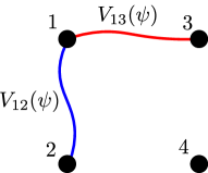
Figure 7: The string operators $V_{12}(\psi)$ and $V_{13}(\psi)$ for four $\sigma\bar{\sigma}$ anyons at points 1, 2, 3, and 4. The string operators $V_{12}(\bar{\psi})$ and $V_{12}(\bar{\psi})$ are analogous.

Let us study this space in more detail. For definiteness, we label the four $\sigma\bar{\sigma}$ anyons as $1,2,3,4$. We denote by $V_{ij}(a)$ the open string operator of $a$ connecting $i$-th and $j$-th $\sigma\bar{\sigma}$. One can label the basis for the four-dimensional space by the eigenvalues of the string operators $V_{12}(\psi)$ and $V_{12}(\bar{\psi})$. The conjugate operators are $V_{13}(\psi)$ and $V_{13}(\bar{\psi})$. See Fig. 7 for an illustration of the string operators. The logical Pauli operators can be defined as X_1&=V_12(ψ),  ​ X_2=V_12(¯ψ),
Z_1=V_13(ψ),  Z_2=V_13(¯ψ). The coherent subspace should have fixed eigenvalue under any nonlocal stabilizers, which include $V_{ij}(\psi\bar{\psi})$. To illustrate, let us assume that $V_{ij}(\psi\bar{\psi})=1$. Observe that V_12(ψ¯ψ) &= V_12(ψ) V_12(¯ψ) =X_1X_2,
V_13(ψ¯ψ) = V_13(ψ)V_13(¯ψ) = Z_1Z_2. Thus, the coherent subspace is satisfies the constraints $X_{1}X_{2}=1$ and $Z_{1}Z_{2}=1$, which is one-dimensional space. In other words, the non-Abelian degeneracy becomes classical: the 4-dimensional Hilbert space is decohered into 4 classical states (i.e. isolated extremal points).

Local indistinguishability on a torus

If the Ising string-net model is defined on a torus, then there are nine locally-indistinguishable ground states. A basis for the ground state space is given by $\{\ket{a}\}$, where $a\in\{1,\psi,\sigma\}\times\{1,\bar{\psi},\bar{\sigma}\}$. We choose the states $\ket{a}$ to be eigenstates of the closed string operators $W_{y}(b)$ along the non-contractible path in the $y$ direction. More specifically, we can choose the states such that

$$W_{y}(b)\ket{a}=\frac{S_{ab}}{S_{Ia}}\ket{a},\quad W_{x}(b)\ket{a}=\sum_{c}N_{ab}^{c}\ket{c},$$ (96)

where $W_{x}(b)$ is the string operator wrapped around the non-contractible path in the $x$ direction.

Before adding noise to the Ising string-net model, it is instructive to first consider coherently condensing the $\psi\bar{\psi}$ anyons. The effect of condensation is that the ground states are projected onto the mutual $+1$ eigenspace of the $\psi\bar{\psi}$ string operators, reflecting the fact that the $\psi\bar{\psi}$ anyons can be freely created and annihilated. Note that, according to Eq. (96), the ground states $\ket{a}$ labeled by anyons that have nontrivial braiding relations with $\psi\bar{\psi}$ are annihilated by the projector. Writing the image of the ground state $|a\rangle$ under the projection as $|a\rangle_{\psi\bar{\psi}}$, we are left with the following three nontrivial states:

$$\ket{I}_{\psi\bar{\psi}},\quad\ket{\sigma\bar{\sigma}}_{\psi\bar{\psi}},\quad\ket{\psi}_{\psi\bar{\psi}}.$$ (97)

Here, the states $\ket{\psi\bar{\psi}}_{\psi\bar{\psi}}$ and $\ket{\bar{\psi}}_{\psi\bar{\psi}}$ have become identified with $\ket{I}_{\psi\bar{\psi}}$ and $\ket{\psi}_{\psi\bar{\psi}}$, respectively.

One might naively conclude that the ground state subspace is three-dimensional. However, there is a fourth basis state, which can be understood as follows. Because of the non-Abelian fusion rule $\sigma\bar{\sigma}\times\psi\bar{\psi}=\sigma\bar{\sigma}$, it is possible to create an excited state on the torus with a single $\psi\bar{\psi}$, as long as there is a $\sigma\bar{\sigma}$ anyon flux threading the torus. We refer to this state as $\ket{\sigma\bar{\sigma}^{(\psi\bar{\psi})}}$. After condensation, this state is locally indistinguishable from the states in Eq. (97), which have an even parity of $\psi\bar{\psi}$ anyons. Thus, the ground state space becomes 4-dimensional. Note that this agrees with the fact that condensing $\psi\bar{\psi}$ produces a model with the same TO as the $\mathbb{Z}_{2}$ TC. In fact, we can make the following identifications:

$$\ket{I}_{\psi\bar{\psi}} \sim\ket{1}_{\rm TC}$$ (98)

$$\ket{\psi}_{\psi\bar{\psi}} \sim\ket{\psi}_{\rm TC}$$ (99)

$$\ket{\sigma\bar{\sigma}}_{\psi\bar{\psi}} \sim\frac{1}{\sqrt{2}}(\ket{e}_{\rm TC}+\ket{m}_{\rm TC})$$ (100)

$$\ket{\sigma\bar{\sigma}^{(\psi\bar{\psi})}} \sim\frac{1}{\sqrt{2}}(\ket{e}_{\rm TC}-\ket{m}_{\rm TC}).$$ (101)

Here $\ket{a}_{\rm TC}$ denotes the $\mathbb{Z}_{2}$ TC ground states.

We now study the locally indistinguishable states obtained by decohering the Ising string-net model.

Given any ground state $\rho=\ket{\Psi}\bra{\Psi}$, we apply the noise channel $\mathcal{N}$ in Eq. (74) to obtain the mixed state $\mathcal{N}(\rho)$. Since the noise incoherently proliferates $\psi\bar{\psi}$ anyons, the mixed state is invariant under conjugation by the string operators $W_{x}(\psi\bar{\psi})$ and $W_{y}(\psi\bar{\psi})$: N(ρ) &= W_x(ψ¯ψ) N(ρ) W_x(ψ¯ψ),
N(ρ) = W_y(ψ¯ψ) N(ρ) W_y(ψ¯ψ). This means that the state $\mathcal{N}(\rho)$ preserves the $W_{x}(\psi\bar{\psi})$ and $W_{y}(\psi\bar{\psi})$ eigenspaces. Thus, it is block diagonalized in the eigenbasis of $W_{x}(\psi\bar{\psi})$ and $W_{y}(\psi\bar{\psi})$. Therefore, the coherent subspaces are labeled by the eigenvalues of the $\psi\bar{\psi}$ string operators. Drawing analogy to the examples in Section III, the string operators $W_{x}(\psi\bar{\psi})$ and $W_{y}(\psi\bar{\psi})$ play the same role as the nonlocal stabilizers of the subsystem code.

Each block of $\mathcal{N}(\rho)$ can be expressed as a mixture of states, each of which is obtained by decohering ground states within an eigenspace of $W_{x}(\psi\bar{\psi})$ and $W_{y}(\psi\bar{\psi})$. In other words, under decoherence, the eigenspaces of these string operators yield extremal points of the manifold of locally indistinguishable states. Therefore, there is a continuum of extremal points, with connected components labeled by the eigenvalues of $W_{x}(\psi\bar{\psi})$ and $W_{y}(\psi\bar{\psi})$. To make the discussion more explicit, the eigenspace with $W_{x}(\psi\bar{\psi})=W_{y}(\psi\bar{\psi})=1$ is given by

• $W_{x}(\psi\bar{\psi})=1$, $W_{y}(\psi\bar{\psi})=1$:

  $$\text{span}\Big{\{}\frac{1}{\sqrt{2}}(\ket{I}+\ket{{\psi\bar{\psi}}}),\quad\ket{\sigma\bar{\sigma}},\quad\frac{1}{\sqrt{2}}(\ket{\psi}+\ket{\bar{\psi}})\Big{\}}.$$ (102)

$W_{\psi\bar{\psi}}^{x}$ and $W_{\psi\bar{\psi}}^{y}$ play the same role as the nonlocal stabilizers.

One might notice that the conclusion so far, is very similar to the case of coherently condensing $\psi\bar{\psi}$. It is thus natural to ask whether the state $|\sigma\bar{\sigma}^{(\psi\bar{\psi})}\rangle$ with a single $\psi\bar{\psi}$ plays any role here. Intuitively, since the $\psi\bar{\psi}$ anyons have been incoherently proliferated, at $p=1/2$ one can not locally detect whether there is a $\psi\bar{\psi}$ anyon. Therefore, we have an exponentially large number of locally-indistinguishable states. However, this phenomenon already shows up in the much simpler decohered TC example as discussed in Section II.4, and only happens at $p=1/2$. Therefore, we do not include the state in the locally indistinguishable space.

For completeness, we list the coherent subspaces for the other eigenvalues of $W_{x}(\psi\bar{\psi})$ and $W_{y}({\psi\bar{\psi}})$.

• $W_{x}(\psi\bar{\psi})=-1$, $W_{y}(\psi\bar{\psi})=1$:

  $$\!\!\!\!\!\!\!\!\!\!\!\!\!\!\!\!\!\!\!\!\!\!\!\!\text{span}\Big{\{}\frac{1}{\sqrt{2}}(\ket{I}-\ket{{\psi\bar{\psi}}}),\quad\frac{1}{\sqrt{2}}(\ket{\psi}-\ket{\bar{\psi}})\Big{\}}$$ (103)

• $W_{x}(\psi\bar{\psi})=1$, $W_{y}(\psi\bar{\psi})=-1$:

  $$\!\!\!\!\!\!\!\!\!\!\!\!\!\!\!\!\!\text{span}\Big{\{}\frac{1}{\sqrt{2}}(\ket{\sigma}+\ket{\sigma\bar{\psi}}),\quad\frac{1}{\sqrt{2}}(\ket{\bar{\sigma}}+\ket{\psi\bar{\sigma}})\Big{\}}$$ (104)

• $W_{x}(\psi\bar{\psi})=-1$, $W_{y}(\psi\bar{\psi})=-1$:

  $$\text{span}\Big{\{}\frac{1}{\sqrt{2}}(\ket{\sigma}-\ket{\sigma\bar{\psi}}),\quad\frac{1}{\sqrt{2}}(\ket{\bar{\sigma}}-\ket{\psi\bar{\sigma}})\Big{\}}.$$ (105)

Notice that each of these subspaces is 2-dimensional. Intuitively, in the pure-state case, these correspond to inserting defect lines along non-contractible paths in the $\mathbb{Z}_{2}$ TC.

For ground state TOs defined on a torus, the locally-indistinguishable ground states transform nontrivially under the modular transformations of the torus. The universal part of the transformation, known as the modular data, is related to the braiding statistics of the anyons. In a lattice model, the modular transformations can be implemented by coordinate transformations Zhang:2011jd. For example, the $S$ transformation corresponds to a $\pi/2$ rotation, which swaps the $x$ and $y$ axes, and the $T$ transformation can be implemented by a shear deformation, or a Dehn twist. The modular matrices can then be found by computing the matrix representations of the corresponding coordinate transformations in the ground-state subspace and removing non-universal contributions.

It is natural to ask how the modular transformations act on the locally-indistinguishable states in mixed-state TOs, such as the decohered doubled Ising TO. To this end, we study the expectation values of the modular transformations on states inside the coherent space. Here we consider both ordinary linear-in-$\rho$ expectation value, as well as the non-linear expectation values. In both cases, we find that up to a normalization factor, the expectation values are equal to the pure state expectation values. Details of the calculations can be found in Appendix LABEL:app:_modular_data.

In the coherent space defined in Eq. (102), we find that the S and T transformations are represented by

$$S=\frac{1}{2}\begin{pmatrix}1&\sqrt{2}&1\\ \sqrt{2}&0&-\sqrt{2}\\ 1&-\sqrt{2}&1\end{pmatrix},\quad T=\begin{pmatrix}1&0&0\\ 0&1&0\\ 0&0&-1\end{pmatrix}.$$ (106)

Curiously, these modular matrices do not correspond to any anyon theory: the S matrix is identical to that of a (chiral) Ising TO, but the T matrix differs in the second diagonal entry from any of the modular anyon theories with the same S matrix.

V.2 $G$-graded string-net models

We now discuss generalizations of the construction of the decohered doubled Ising state in the previous section. We begin by further introducing details about string-net models. For a general string-net model, the input data is a unitary fusion category $\mathcal{C}$. On each edge of the lattice, one has a local Hilbert space with an orthonormal basis labeled by simple objects (also referred to as “string types”) of $\mathcal{C}$. Each vertex of the lattice corresponds to a fusion of the three strings on the edges emanating from the vertex. A string-net state is a basis state (i.e., a configuration of string labels on the edges) that satisfies the fusion rules of $\mathcal{C}$ at all vertices.

The commuting-projector Hamiltonian is given by

$$H=-\sum_{v}A_{v}-\sum_{p}B_{p},$$ (107)

which is a generalization of Eq. (69). Here $A_{v}$ is a vertex projector that enforces the fusion rule at each vertex $v$. The plaquette term $B_{p}$ takes the following form

$$B_{p}=\frac{1}{\mathcal{D}^{2}}\sum_{a}d_{a}B_{p}^{a},$$ (108)

where $B_{p}^{a}$ pictorially fuses a loop of $a$ string type to a plaquette $p$. Furthermore, $d_{a}$ is the quantum dimension of $a$ and $\mathcal{D}$ is the total quantum dimension. For details, we refer to Ref. Lin:2020bak.

The ground state wave function of the string-net model is a certain coherent superposition of all string-net states that satisfies $B_{p}=1$ (and $B_{p}^{a}=d_{a}$). The relative amplitudes of the string-net states are determined by a set of local rules, which involve further categorical data (e.g. $F$-symbols) of $\mathcal{C}$. The TO in the ground state is described by the so-called Drinfeld center $\mathcal{Z}(\mathcal{C})$.

We can further assume that the input category is $G$-graded, where $G$ is taken to be a finite group. A $G$-graded fusion category $\mathcal{C}$ has the following decomposition:

$$\mathcal{C}=\bigoplus_{\mathbf{g}\in G}\mathcal{C}_{\mathbf{g}},$$ (109)

such that $\mathcal{C}_{\mathbf{g}}\times\mathcal{C}_{\mathbf{g}}\subset\mathcal{C}_{\mathbf{gh}}$. In other words, fusion rules in $\mathcal{C}$ respect the $G$-grading:

$$a_{\mathbf{g}}\times b_{\mathbf{h}}=\sum_{c_{\mathbf{gh}}\in\mathcal{C}_{\mathbf{gh}}}N_{a_{\mathbf{g}}b_{\mathbf{h}}}^{c_{\mathbf{gh}}}c_{\mathbf{gh}}.$$ (110)

We say that $\mathcal{C}$ is a $G$-extension of $\mathcal{C}_{1}$, the identity component.

A particularly useful fact is that the TO $\mathcal{Z}(\mathcal{C})$ can be obtained from $\mathcal{Z}(\mathcal{C}_{1})$ by gauging a $G$ symmetry. This means that $\mathcal{Z}(\mathcal{C})$ contains a subcategory of (possibly non-Abelian) bosons isomorphic to $\operatorname{Rep}(G)$, the category of finite-dimensional linear representations of $G$. Physically, $\operatorname{Rep}(G)$ describes the $G$ charges of the gauge theory. Condensing $\operatorname{Rep}(G)$ in $\mathcal{Z}(\mathcal{C})$ again yields $\mathcal{Z}(\mathcal{C}_{1})$. Based on this relation, Refs. HeinrichPRB2016 and ChengSET2017 constructed exactly solvable models for SET phases whose underlying topological order is given by $\mathcal{Z}(\mathcal{C}_{1})$, and such that gauging the $G$ symmetry yields thte TO $\mathcal{Z}(\mathcal{C})$.

As an example, the Ising fusion category is $\mathbb{Z}_{2}=\{1,\mathbf{g}\}$ graded, with $\mathcal{C}_{1}=\{1,\psi\}$ and $\mathcal{C}_{\mathbf{g}}=\{\sigma\}$. The Drinfeld center $\mathcal{Z}(\mathcal{C})$ is the doubled Ising TO, which is related to the $\mathbb{Z}_{2}$ TC (the Drinfeld center $\mathcal{Z}(\mathcal{C}_{1})$), by gauging the $\mathbb{Z}_{2}$ symmetry that permutes the $e$ and $m$ anyons.

We now use the $G$-graded string-net models to produce examples of mixed states with mixed-state TO, similar to the construction with the Ising string-net model. We start from the ground state $\rho_{0}=\ket{\Psi}\!\bra{\Psi}$ of the string-net model for $\mathcal{C}$. Because of the $G$-graded structure of $\mathcal{C}$, the $G$-grading labels on the edges should form a $G$-defect network. For a given $G$-defect network $\{\mathbf{g}\}$, we define a projector $P(\{\mathbf{g}\})$, and let

$$\ket{\Psi_{\{\mathbf{g}\}}}=P(\{\mathbf{g}\})\ket{\Psi}.$$ (111)

The fixed-point density matrix is given by

$$\rho_{G}\propto\sum_{\{\mathbf{g}\}}\ket{\Psi_{\{\mathbf{g}\}}}\!\bra{\Psi_{\{\mathbf{g}\}}}.$$ (112)

For the Ising fusion category, the projector $P(\{\mathbf{g}\})$ is a projector onto a fixed configuration of $\sigma$ loops, and the state $\rho_{G}$ is a mixture of these configurations.

The mixed state $\rho_{G}$ can be obtained from $\rho_{0}$ using the QLC $\mathcal{N}$ defined below – thus, $\rho_{G}$ has a purification into a GGS. The QLC $\mathcal{N}$ is defined as:

$${\mathcal{N}}=\prod_{e}{\mathcal{N}}_{e},\quad{\mathcal{N}}_{e}(\rho)=\frac{1}{|G|}\sum_{\mathbf{g}\in G}T_{e}^{\mathbf{g}}\rho T_{e}^{\mathbf{g}}.$$ (113)

Here, the operator $T^{\mathbf{g}}$ (suppressing the edge label) is given by

$$\begin{split}T^{\mathbf{g}}\ket{a_{\mathbf{h}}}=\delta_{\mathbf{g,h}}\ket{a_{\mathbf{h}}}.\end{split}$$ (114)

The string-net ground state has the following density matrix:

$$\rho_{0}=\prod_{v}A_{v}\prod_{p}B_{p}.$$ (115)

After applying the channel, it becomes

$$\mathcal{N}(\rho)\propto\prod_{v}A_{v}\prod_{p}\Big{(}\sum_{a\in\mathcal{C}_{1}}d_{a}B_{p}^{a}\Big{)},$$ (116)

which is an equivalent representation of $\rho_{G}$.

Physically, as will be explained in more details later in Section V.3, these $T^{\mathbf{g}}$ operators create gauge charges, which are labeled by irreducible representations of $G$. $\rho_{G}$ is thus obtained from $\rho_{0}$ by incoherently proliferating the gauge charges. Note that, when $G$ is a non-Abelian group, the gauge charges may be non-Abelian.

We also note that, in the special case when the input category is just the group algebra ${\rm Vec}_{G}$ (i.e. $\mathcal{C}_{\mathbf{g}}=\{\mathbf{g}\}$), the string-net model is equivalent to the Kitaev’s quantum double model Kitaev:1997wr. In this case, the density matrix in Eq. (112) describes a classical ensemble of $G$ gauge fields, i.e., a classical $G$ gauge theory Liu:2023opg. We use this observation in the next section to generalize the construction beyond $G$-graded string-net models.

We now discuss another way to prepare the state $\rho_{G}$, generalizing the observations about the decohered doubled Ising model in Section V.1.

In particular, we show that $\rho_{G}$ can always be purified into a symmetry-enriched $\mathcal{Z}(\mathcal{C}_{1})$ state, meaning that $\rho_{G}$ can be prepared by tracing out certain degrees of freedom in the SET state. Intuitively, the state $\ket{\Psi_{\{\mathbf{g}\}}}$ can be viewed as the ground state of the $\mathcal{C}_{1}$ string-net model but with insertions of topological defects. $\rho_{G}$ is then a classical mixture of ground states with defects, similar to the decohered doubled Ising state in Section V.1.

To see the purifications explicitly, we follow Refs. ChengSET2017; HeinrichPRB2016 and begin by introducing plaquette $G$ spins with an orthonormal basis $\ket{\mathbf{g}}$, for $\mathbf{g}\in G$. The string-net Hamiltonian is then modified as follows. For each edge, we introduce a projector that aligns the $G$-grading of the edge with the domain wall of the adjacent plaquette spins. The plaquette term is also modified to

$$B_{p}=\frac{1}{\mathcal{D}^{2}}\sum_{a_{\mathbf{g}}\in\mathcal{C}}d_{a_{\mathbf{g}}}L_{p}^{\mathbf{g}}B_{p}^{a_{\mathbf{g}}}=\frac{1}{|G|}\sum_{\mathbf{g}}L_{p}^{\mathbf{g}}B_{p}^{\mathbf{g}},$$ (117)

where $L_{p}^{\mathbf{g}}$ acts as left multiplication: $L_{p}^{\mathbf{g}}\ket{\mathbf{g}_{p}}=\ket{\mathbf{g}\mathbf{g}_{p}}$. We have also defined

$$B_{p}^{\mathbf{g}}=\frac{1}{\mathcal{D}_{1}^{2}}\sum_{a_{\mathbf{g}}\in\mathcal{C}_{\mathbf{g}}}d_{a_{\mathbf{g}}}B_{p}^{a_{\mathbf{g}}}.$$ (118)

The operator $B_{p}$ fluctuates the plaquette spins and changes the grading on the edges to abide by the edge projectors. We note that the operators $B_{p}^{\mathbf{g}}$ obey the following relations:

$$\begin{split}B_{p}^{\mathbf{g}}B_{p}^{\mathbf{h}}&=B_{p}^{\mathbf{gh}},\\ B_{p}^{\overline{\mathbf{g}}}&=(B_{p}^{\mathbf{g}})^{\dagger}\\ [B_{p}^{\mathbf{g}},B^{\mathbf{h}}_{p^{\prime}}]&=0,\text{ for }p\neq p^{\prime},\end{split}$$ (119)

with $\overline{\mathbf{g}}$ defined as

$$\bar{\mathbf{g}}\equiv\mathbf{g}^{-1}.$$ (120)

These properties of $B_{p}^{\mathbf{g}}$ essentially follow from the properties of plaquette operators of string-net models, proven in Appendix D of Ref. Lin:2020bak. The Hamiltonian is invariant under $U_{\mathbf{g}}=\prod_{p}R_{p}^{\mathbf{g}}$, where $R_{p}^{\mathbf{g}}\ket{\mathbf{g}_{p}}=\ket{\mathbf{g}_{p}\mathbf{g}}$.

When the system is defined on a sphere, the ground state wave function can be written as

$$\ket{\Psi_{\rm SET}}=\frac{1}{\sqrt{|G|}}\sum_{\{\mathbf{g}_{p}\}}\ket{\{\mathbf{g}_{p}\}}\otimes\ket{\Psi_{\{\partial\mathbf{g}_{p}\}}},$$ (121)

where $\ket{\Psi_{\{\mathbf{g}\}}}$ is defined in Eq. (111), and $\{\partial\mathbf{g}_{p}\}$ refers to the $G$ defects defined by the $\{\mathbf{g}_{p}\}$ domain walls. After tracing out the plaquette spins, we are left with the state $\rho_{G}$. Therefore, $\ket{\Psi_{\rm SET}}$ is a purification of $\rho_{G}$, as claimed.

The fact that the mixed state $\rho_{G}$ can be purified into an SET state suggests a potential generalization of the construction. In particular, we can build an analog of $\rho_{G}$ starting from a SET mixed state, as opposed to a pure state. This allows for additional possibilities, due to the fact that mixed states can be enriched by weak symmetries, which do not suffer from t’ Hooft anomalies Ma:2022pvq. As a consequence, there are SET mixed states with anomalous $G$ symmetries that do not have any pure-state counterpart with an onsite $G$ symmetry. In the next section, we construct mixed-state TOs from $G$ SET states, which may have an t’ Hooft anomaly, by “classically gauging” the symmetry.

Figure 8: Commutative diagram for the two constructions of mixed states in Sections V.2 and V.3. The diagram is commutative when the $G$ SET order admits a gapped boundary and $G$ is non-anomalous. (a) The construction in Section V.2 can be interpreted as starting with a non-anomalous $G$ SET state with gapped boundaries, such as those from Refs. ChengSET2017; HeinrichPRB2016, and (quantum) gauging the $G$ symmetry. We have used a dashed line, as a reminder that this is only possible if the $G$ symmetry is non-anomalous. This results in the TO of a $G$-graded string-net model. (b) Starting from a $G$-graded string-net model, we add noise to transform coherent fluctuations of the $G$-gradings into incoherent fluctuations. Equivalently, the process can be viewed as incoherent proliferation of anyons in the $\operatorname{Rep}(G)$ subtheory. (c) Starting from an arbitrary SET state (which may be anomalous or not admit a gapped boundary), the global symmetry can be classically gauged to obtain a mixed state characterized by the $G$ symmetrization of the SET order.

V.3 Classically gauging SET orders

It has been well-established by now that gauging (generalized) global symmetries is a powerful tool for relating certain pure state TOs to one another. For example, gauging a finite 0-form symmetry in an SPT state gives a topological gauge theory, while gauging a finite 0-form symmetry in an SET state leads to a new TO with a gauge structure SET; TeoSET2015. Here, we interpret the decohered string-net states discussed in the previous section in terms of “classically gauging” weak symmetries. We then argue that this procedure can be applied to more general SET states beyond the string-net constructions, e.g., chiral TOs.

First, we describe what we mean by classical gauging at a conceptual level. To draw a comparison, we start by reviewing the standard (quantum-mechanical) gauging. Suppose we have a pure many-body state $\ket{\psi}$, invariant under a (strong) finite-group symmetry $G$. We additionally assume that the symmetry is implemented by finite-depth local-unitary circuits. The first step in gauging is to couple the system to background gauge fields of the $G$ symmetry. In other words, symmetry defects associated with a flat background gauge field are inserted by acting with the symmetry in a (generally disconnected) region $R$ and flipping the gauge fields on the boundary of $R$. Thus, for each background gauge field, schematically denoted by $A$, we have a state $\ket{\psi(A)}$.

Next, in gauging the symmetry of the pure many-body state, one forms a coherent superposition of the states with defects, summing over all possible defect configurations:

$$\ket{\psi_{G}}\propto\sum_{A}e^{i\alpha(A)}\ket{\psi(A)}.$$ (122)

Here, the weight $e^{i\alpha(A)}$ is a phase factor that depends locally on $A$, known as the “local counterterm” in the field theory literature. In order for this superposition to make sense as a gauge-invariant state, $e^{i\alpha(A)}\ket{\psi(A)}$ must be single-valued over the space of $A$. If this can not be achieved with any choice of the local counterterm $\alpha(A)$, then we say there is an obstruction to gauging. In other words, the symmetry has an ’t Hooft anomaly. This step is equivalent to imposing Gauss’s law strongly.

Now, we modify this procedure to define how to classically gauge a weak symmetry group ${G}$ of a mixed state $\rho$. The first step of the procedure remains essentially the same: for each background gauge field $A$ (or equivalently, insertion of symmetry defects), one can canonically define a state $\rho(A)$. The next step is now considerably more straightforward: we simply form a classical mixture

$$\rho_{G}\propto\sum_{A}\rho(A).$$ (123)

Notice that there is no issue with anomalous phase factors in this case, since the Gauss’s laws are only imposed weakly. That is, the mixed state is only required to be invariant under the conjugation by local gauge transformations.

V.3.1 Classical gauging in string-net states

Let us spell out classical gauging more concretely by reproducing the mixed state $\rho_{G}$ from the previous section, this time through classical gauging. We start with a weak SET state $\rho_{\rm wSET}$ derived from the SET state in Eq. (121):

$$\rho_{\rm wSET}\propto\sum_{\{\mathbf{g}_{p}\}}\ket{\{\mathbf{g}_{p}\}}\!\bra{\{\mathbf{g}_{p}\}}\otimes\rho_{\rm SN}(\{\partial\mathbf{g}_{p}\}),$$ (124)

where $\rho_{\rm SN}(\{\partial\mathbf{g}_{p}\})$ is the $\mathcal{C}_{1}$ string-net state with defects

$$\rho_{\rm SN}(\{\partial\mathbf{g}_{p}\})=\ket{\Psi_{\{\partial\mathbf{g}_{p}\}}}\!\bra{\Psi_{\{\partial\mathbf{g}_{p}\}}}.$$ (125)

Note that the weak SET state $\rho_{\rm wSET}$ is obtained from $\ket{\Psi_{\rm SET}}$ in Eq. (121) by dephasing the $G$ spins. This reduces the strong $G$ symmetry to a weak $G$ symmetry.

Now, we follow the steps above to classically gauge the weak $G$ symmetry. The first step is to add gauge fields, which is accomplished by adding a $G$ spin to each edge of the lattice. We then insert a configuration of topological defects corresponding to $\{\mathbf{h}_{p}\}$ to obtain &ρ_wSET({h_p}) ∝
      ∑_{g_p}|{h_pg_p}⟩​⟨{h_pg_p}|⊗ρ_SN({∂g_p}) ⊗ρ_GF({∂h