Thermodynamics of Non-Hermitian Josephson junctions with exceptional points
Abstract
We present an analytical formulation of the thermodynamics, free energy and entropy, of any generic Bogoliubov de Genes model which develops exceptional point (EP) bifurcations in its complex spectrum when coupled to reservoirs. We apply our formalism to a non-Hermitian Josephson junction where, despite recent claims, the supercurrent does not exhibit any divergences at EPs. The entropy, on the contrary, shows a universal jump of which can be linked to the emergence of Majorana zero modes (MZMs) at EPs. Our method allows us to obtain precise analytical boundaries for the temperatures at which such Majorana entropy steps appear. We propose a generalized Maxwell relation linking supercurrents and entropy which could pave the way towards the direct experimental observation of such steps in e.g. quantum-dot based minimal Kitaev chains.
Introduction–At weak coupling, an external environment only induces broadening and small shifts to the levels of a quantum system. In contrast, the strong coupling limit is highly nontrivial and gives rise to many interesting concepts in e.g. quantum dissipation Weiss (2021), quantum information science Harrington et al. (2022) or quantum thermodynamics Rivas (2020), just to name a few. An interesting example is the emergence of spectral degeneracies in the complex spectrum (resulting from integrating out the environment), also known as exceptional point (EP) bifurcations, where eigenvalues and eigenvectors coalesce Berry (2004). During the last few years, a great deal of research is being developed in so-called non-Hermitian (NH) systems with EPs, in various contexts including open photonic systems Doppler et al. (2016), Dirac Zhen et al. (2015), Weyl Cerjan et al. (2019) and topological matter in general Shen et al. (2018); Gong et al. (2018); Kawabata et al. (2019); Bergholtz et al. (2021).
The role of NH physics and EP bifurcations in systems with Bogoliubov-de Gennes (BdG) symmetry has hitherto remained unexplored, until recently. Specifically, there is an ongoing debate on how to correctly calculate the free energy in open BdG systems, a question relevant in e.g Josephson junctions coupled to external electron reservoirs. Depending on different approximations, such "NH junctions" have been predicted to exhibit exotic effects including imaginary persistent currents Zhang et al. (2022); Li et al. (2021) and supercurrents Cayao and Sato (2023); Li et al. (2024) or various transport anomalies at EPs Kornich (2023). If one instead uses the biorthogonal basis associated with the NH problem Shen et al. (2024), or an extension of scattering theory to include external electron reservoirs Beenakker (2024), the supercurrents are real and exhibit no anomalies. At the heart of this debate is whether a straightforward use of the complex spectrum plugged into textbook definitions of thermodynamic functions leads to meaningful results or whether, on the contrary, NH physics needs to be treated with care when calculating the free energy.
We here present a well-defined procedure, valid for arbitrary coupling and temperature, which allows us to calculate the free energy, Eq. (4), without any divergences at EPs. Derivatives of this free energy, allow us to calculate physical observables such as entropy (6) or supercurrents (7). Interestingly, entropy changes of can be connected to emergent Majorana zero modes (MZMs) at EPs Pikulin and Nazarov (2013); San-Jose et al. (2016); Avila et al. (2019). While such fractional entropy steps were predicted before in seemingly different contexts Smirnov (2015); Sela et al. (2019); Becerra et al. (2023), our analysis in terms of EPs allows us to obtain precise analytical boundaries for the temperatures at which they appear. We propose a novel Maxwell relation connecting supercurrents and entropy, Eq. (12), which would allow the experimental detection of the effects predicted here.
Exceptional points in open BdG models– The starting point of our analysis is the description of the open quantum system in terms of a Green’s function
| (1) |
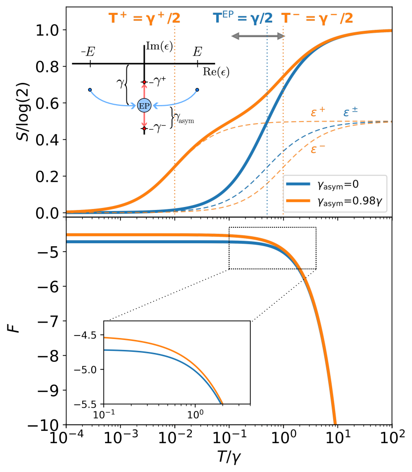
where is an effective NH Hamiltonian which takes into account how the quantum system is coupled to an external environment through the retarded self-energy . In what follows, we consider the case where an electron reservoir induces a tunneling rate 111We consider the simplest case where this selfenergy originates from a tunneling coupling to an external electron reservoir in the so-called wideband approximation where both the tunneling amplitudes and the density of states in the reservoir are energy independent, which allows to write the tunneling couplings as constant Meir and Wingreen (1992)., such that the complex poles of Eq. (1) have a well-defined physical interpretation in terms of quasi-bound states. If is a BdG Hamiltonian, electron-hole symmetry can be satisfied in two non-equivalent ways: (i) one can have pairs of poles with opposite real parts and with the same imaginary part ; or, alternatively, (ii) two independent and purely imaginary poles . A bifurcation of the former, corresponding to standard finite-energy BdG modes with an equal decay to the reservoir , into the latter, two MZMs with different decay rates Pikulin and Nazarov (2013); San-Jose et al. (2016); Avila et al. (2019), defines an EP (Fig. 1a, inset).
NH Free energy– Calculating the free energy of an open quantum system is nontrivial since a direct substitution of a complex spectrum in the standard expression , can lead to complex results and divergences after an EP Cayao and Sato (2023); Li et al. (2024). To avoid inconsistencies, one possibility is to use the occupation , which is a well-defined quantity in open quantum systems, even in non-equilibrium situations where the so-called Keldysh lesser Green’s function can be generalized beyond the fluctuation-dissipation theorem Meir and Wingreen (1992). In BdG language, can be written as
| (2) |
where is the Fermi-Dirac function and we have explicitly separated the total spectral function
| (3) |
in its particle () and hole () branches, and , respectively 222A global factor of arises from the duplicity of dimensions in BdG formalism.. We have also added a Lorentzian cutoff to avoid divergences in the thermodynamic quantities as (see Supplemental Material Sup ). The integral in Eq. (2) can be analytically solved by residues Sup and then be used to obtain as:
| (4) | ||||
with being the log-gamma function and a generic function coming from the integration. We now perform the limits and of the previous expression,
| (5) | ||||
which, by comparison with well-known limits Zagoskin (2014); Hewson (1993), give 333Interestingly, this term is relevant for the entropy since it adds a physical contribution . In contrast, the term cancels out in the supercurrent Sup .. From now on, we fix but the complete derivation with full expressions, including , can be found in Sup . Derivatives of Eq. (4) allow us to obtain relevant thermodynamic quantities, as we discuss now.
Entropy steps from EPs– Using the free energy in Eq. (4), the entropy, defined as , reads:
| (6) | ||||
where is the digamma function. From Eq. (6), we can define a critical temperature as the inflection point when the eigenvalue begins to have a non-zero contribution () to the total entropy, Fig. 1 (top). Hence, two standard BdG poles will contribute at the same temperature to the entropy of the system since their absolute values are equal, , and thus a single plateau of can be measured. On the contrary, after an EP at , the poles bifurcate taking zero real parts and different imaginary parts, and , and separating from each other a distance . Then, each pole will contribute to the entropy at a different temperature , giving rise to a fractional plateau of width . Here it is very important to point out that this nontrivial behavior of the entropy seems absent in the free energy that we used for the calculation of . Indeed, is seemingly insensitive to any EP bifurcation even when varying the temperature over six decades, Fig. 1 (bottom).
Non-Hermitian Josephson junction with EPs– Our method also allows to calculate the supercurrent of any generic NH Josephson junction (or similarly the persistent current through a normal ring Shen et al. (2024)) by just considering a phase-dependent spectrum and taking phase derivatives of Eq. (4) as , which gives
| (7) | ||||
As , the supercurrent carried by a pair of BdG poles simply becomes 444For a single pair of BdG poles, is independent/dependent of the phase before/after the EP and the other way around for Sup .
| (8) | ||||
which, for example, allows us to calculate the supercurrent carried by Andreev levels in a short junction coupled to an electron reservoir almost straigthforwardly Sup . Note that, although has a cutoff-dependent term, it cancels by the particle-hole symmetry of the problem Sup . Eqs. (8) strongly differ from a calculation using directly the complex spectrum Cayao and Sato (2023); Li et al. (2024)
| (9) |
Eqs. (4), (6) and (7) are the main results of this paper and allow to calculate thermodynamics from generic open BdG models (arbitrary coupling and temperature) that can be written in terms of complex poles (Eq. (1)).
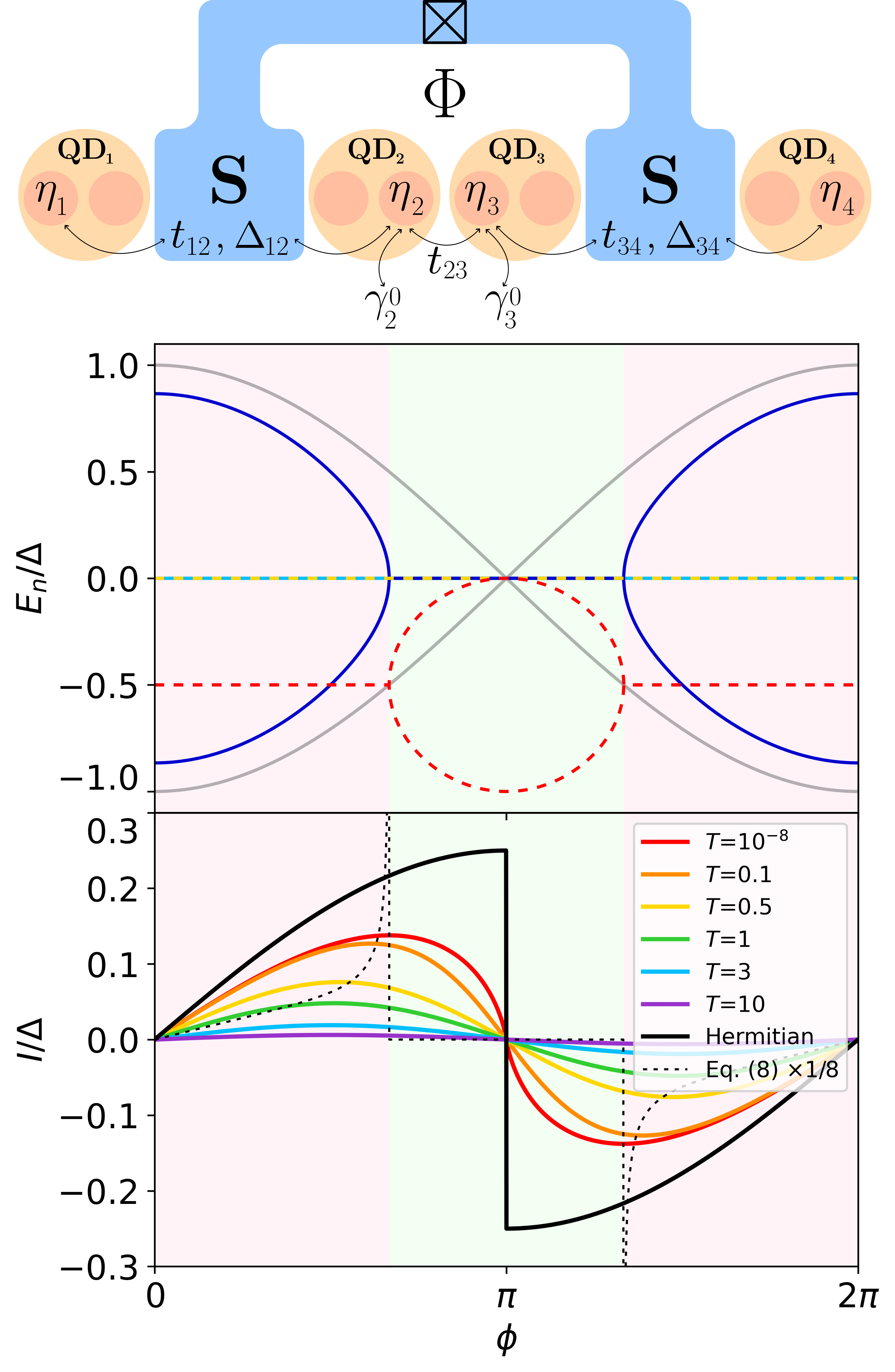
Non-Hermitian minimal Kitaev Josephson junction– As an application we now consider a quantum dot (QD) array in a so-called minimal Kitaev model
| (10) |
where () denote creation (annihilation) operators on each QD with a chemical potential . The QDs couple via a common superconductor that allows for crossed Andreev reflection and single-electron elastic co–tunneling, with coupling strengths and , respectively. Remarkably, only two QDs are enough to host two localized MZMs and when a so-called sweet spot is reached with . This theoretical prediction Leijnse and Flensberg (2012) has recently been experimentally implemented Dvir et al. (2023); ten Haaf et al. (2024). Let consider now a second double QD array (Majoranas and ) that forms a Josephson junction with the former array with a coupling , with being the superconducting phase difference between both arrays and the tunneling coupling between inner QDs. If, additionally, the two inner QDs are coupled to normal reservoirs with rates and this system is a realization of a Non-Hermitian Josephson junction containing Majorana modes (see the sketch in Fig. 2 top). In the low-energy regime, this model can be described in terms of four Majorana modes Pino et al. (2024). Assuming and and , only the inner Majoranas and are coupled and lead to BdG fermionic modes of energy , where , and , while the outer modes remain completely decoupled and . For , one recovers the standard Majorana Josephson term: . When , the spectrum develops EPs at phases For an example of the resulting supercurrents and a comparison against Eq. (9), see Fig. 2 bottom. Similarly, when , but , an additional pair of EPs appears at 555Analytical expressions of eigenvalues, a similar calculation for a junction containing Andreev levels, as well as detailed discussions can be found in the Sup . .
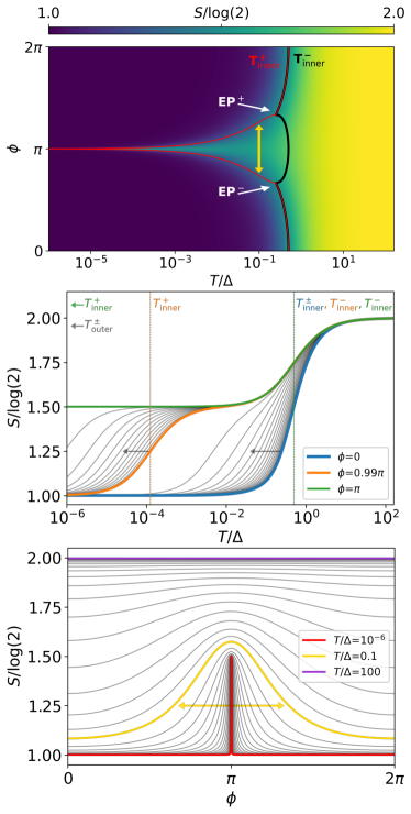
Using these analytics, the critical temperatures read
| (11) | ||||
To illustrate their physical meaning, we plot a full calculation of the entropy using Eq. (6), Fig. 3 top, together with the analytical expressions in Eq. (11) (solid lines). This plot demonstrates that changes in entropy can be understood from EPs, a claim that is even clearer by analyzing cuts at fixed phase (Fig. 3 center). Interestingly, a universal entropy change of can be linked to the emergence of MZMs at phase as . Alternatively, the entropy loss due to Majoranas can be seen in phase-dependent cuts taken at different temperatures, Fig. 3 bottom, which show as an interesting behavior where a plateau at large temperatures becomes an emergent narrow resonance, centered at and of height , as is lowered.
Experimental detection of fractional entropy– recently it has been demonstrated that one can measure entropies of mesoscopic systems, either via Maxwell relations Hartman et al. (2018); Child et al. (2022) or via thermopower Kleeorin et al. (2019); Pyurbeeva et al. (2021). The Maxwell relation method relies on continuously changing a parameter (e.g. chemical potential or magnetic field) while measuring its conjugate variable (e.g. electron number or magnetization, respectively) such that . Then, the Maxwell relation yields . Here we propose a novel application of this procedure, employing the Josephson current , which gives
| (12) |
Since the phase difference on the Josephson junction can be controlled by e.g. embedding it in a SQUID loop Bargerbos et al. (2023); Pita-Vidal et al. (2023), Fig. 2 top, one can integrate between and . From Fig. 3 (bottom) we expect to change from zero at high-T to at low-T, an unequivocal signature of Majorana zero modes in the junction.
Acknowledgements–DMP and RA acknowledge financial support from the Horizon Europe Framework Program of the European Commission through the European Innovation Council Pathfinder Grant No. 101115315 (QuKiT), the Spanish Ministry of Science through Grants No. PID2021-125343NB-I00 and No. TED2021-130292B-C43 funded by MCIN/AEI/10.13039/501100011033, “ERDF A way of making Europe” and European Union Next Generation EU/PRTR, as well as the CSIC Interdisciplinary Thematic Platform (PTI+) on Quantum Technologies (PTI-QTEP+). YM acknowledges support from the European Research Council (ERC) under the European Unions Horizon 2020 research and innovation programme under Grant Agreement No. 951541 and the Israel Science Foundation Grant No. 154/19.
Note added While finishing this manuscript, two recent preprints in Arxiv Shen et al. (2024) and Beenakker (2024) also pointed out the subtleties of calculating the free energy in a NH Josephson junction. Eq. (9) in Ref. Shen et al. (2024) for the supercurrent agrees with our Eq. (7) in the limit without cutoffs . Moreover, Eq. (16) in Ref. Beenakker (2024) agrees with our Eq. (7) in the regime without EPs. This latter case, in particular, results in a reduction factor in the supercurrent, see Eq. (8), owing to the coupling with the reservoir.
References
- Weiss (2021) U. Weiss, Quantum Dissipative Systems (World Scientific Pub Co Inc; 5th edition, 2021).
- Harrington et al. (2022) P. M. Harrington, E. J. Mueller, and K. W. Murch, Nature Reviews Physics 4, 660 (2022), URL https://doi.org/10.1038/s42254-022-00494-8.
- Rivas (2020) A. Rivas, Phys. Rev. Lett. 124, 160601 (2020), URL https://link.aps.org/doi/10.1103/PhysRevLett.124.160601.
- Berry (2004) M. V. Berry, Czechoslovak Journal of Physics 54, 1039 (2004), URL https://doi.org/10.1023/B:CJOP.0000044002.05657.04.
- Doppler et al. (2016) J. Doppler, A. A. Mailybaev, J. Böhm, U. Kuhl, A. Girschik, F. Libisch, T. J. Milburn, P. Rabl, N. Moiseyev, and S. Rotter, Nature 537, 76 (2016).
- Zhen et al. (2015) B. Zhen, C. W. Hsu, Y. Igarashi, L. Lu, I. Kaminer, A. Pick, S.-L. Chua, J. D. Joannopoulos, and M. Soljačić, Nature 525, 354 (2015).
- Cerjan et al. (2019) A. Cerjan, S. Huang, M. Wang, K. P. Chen, Y. Chong, and M. C. Rechtsman, Nature Photonics 13, 623 (2019).
- Shen et al. (2018) H. Shen, B. Zhen, and L. Fu, Phys. Rev. Lett. 120, 146402 (2018), URL https://link.aps.org/doi/10.1103/PhysRevLett.120.146402.
- Gong et al. (2018) Z. Gong, Y. Ashida, K. Kawabata, K. Takasan, S. Higashikawa, and M. Ueda, Phys. Rev. X 8, 031079 (2018), URL https://link.aps.org/doi/10.1103/PhysRevX.8.031079.
- Kawabata et al. (2019) K. Kawabata, K. Shiozaki, M. Ueda, and M. Sato, Phys. Rev. X 9, 041015 (2019), URL https://link.aps.org/doi/10.1103/PhysRevX.9.041015.
- Bergholtz et al. (2021) E. J. Bergholtz, J. C. Budich, and F. K. Kunst, Rev. Mod. Phys. 93, 015005 (2021), URL https://link.aps.org/doi/10.1103/RevModPhys.93.015005.
- (12) See supplemental material at http://link.aps.org/ supplemental/ for further details on.
- Zhang et al. (2022) S.-B. Zhang, M. M. Denner, T. c. v. Bzdušek, M. A. Sentef, and T. Neupert, Phys. Rev. B 106, L121102 (2022), URL https://link.aps.org/doi/10.1103/PhysRevB.106.L121102.
- Li et al. (2021) Q. Li, J.-J. Liu, and Y.-T. Zhang, Phys. Rev. B 103, 035415 (2021), URL https://link.aps.org/doi/10.1103/PhysRevB.103.035415.
- Cayao and Sato (2023) J. Cayao and M. Sato (2023), eprint 2307.15472.
- Li et al. (2024) C.-A. Li, H.-P. Sun, and B. Trauzettel (2024), eprint 2307.04789.
- Kornich (2023) V. Kornich, Phys. Rev. Lett. 131, 116001 (2023), URL https://link.aps.org/doi/10.1103/PhysRevLett.131.116001.
- Shen et al. (2024) P.-X. Shen, Z. Lu, J. L. Lado, and M. Trif (2024), eprint 2403.09569.
- Beenakker (2024) C. W. J. Beenakker (2024), eprint 2404.13976.
- Pikulin and Nazarov (2013) D. I. Pikulin and Y. V. Nazarov, Phys. Rev. B 87, 235421 (2013), URL https://link.aps.org/doi/10.1103/PhysRevB.87.235421.
- San-Jose et al. (2016) P. San-Jose, J. Cayao, E. Prada, and R. Aguado, Scientific Reports 6, 21427 (2016).
- Avila et al. (2019) J. Avila, F. Peñaranda, E. Prada, P. San-Jose, and R. Aguado, Communications Physics 2, 133 (2019), ISSN 2399-3650, URL https://doi.org/10.1038/s42005-019-0231-8.
- Smirnov (2015) S. Smirnov, Phys. Rev. B 92, 195312 (2015).
- Sela et al. (2019) E. Sela, Y. Oreg, S. Plugge, N. Hartman, S. Lüscher, and J. Folk, Phys. Rev. Lett. 123, 147702 (2019), URL https://link.aps.org/doi/10.1103/PhysRevLett.123.147702.
- Becerra et al. (2023) V. F. Becerra, M. Trif, and T. Hyart, Phys. Rev. Lett. 130, 237002 (2023), URL https://link.aps.org/doi/10.1103/PhysRevLett.130.237002.
- Meir and Wingreen (1992) Y. Meir and N. S. Wingreen, Phys. Rev. Lett. 68, 2512 (1992), URL https://link.aps.org/doi/10.1103/PhysRevLett.68.2512.
- Zagoskin (2014) A. Zagoskin, Quantum Theory of Many-Body Systems: Techniques and Applications (Springer, 2014).
- Hewson (1993) A. C. Hewson, The Kondo Problem to Heavy Fermions, Cambridge Studies in Magnetism (Cambridge University Press, 1993).
- Bargerbos et al. (2023) A. Bargerbos, M. Pita-Vidal, R. Žitko, L. J. Splitthoff, L. Grünhaupt, J. J. Wesdorp, Y. Liu, L. P. Kouwenhoven, R. Aguado, C. K. Andersen, et al., Phys. Rev. Lett. 131, 097001 (2023), URL https://link.aps.org/doi/10.1103/PhysRevLett.131.097001.
- Pita-Vidal et al. (2023) M. Pita-Vidal, A. Bargerbos, R. Žitko, L. J. Splitthoff, L. Grünhaupt, J. J. Wesdorp, Y. Liu, L. P. Kouwenhoven, R. Aguado, B. van Heck, et al., Nature Physics 19, 1110 (2023).
- Leijnse and Flensberg (2012) M. Leijnse and K. Flensberg, Phys. Rev. B 86, 134528 (2012).
- Dvir et al. (2023) T. Dvir, G. Wang, N. van Loo, C.-X. Liu, G. P. Mazur, A. Bordin, S. L. D. ten Haaf, J.-Y. Wang, D. van Driel, F. Zatelli, et al., Nature 614, 445 (2023).
- ten Haaf et al. (2024) S. L. D. ten Haaf, Q. Wang, A. M. Bozkurt, C.-X. Liu, I. Kulesh, P. Kim, D. Xiao, C. Thomas, M. J. Manfra, T. Dvir, et al. (2024), eprint 2311.03208.
- Pino et al. (2024) D. M. Pino, R. S. Souto, and R. Aguado, Phys. Rev. B 109, 075101 (2024), URL https://link.aps.org/doi/10.1103/PhysRevB.109.075101.
- Hartman et al. (2018) N. Hartman, C. Olsen, S. Lüscher, M. Samani, S. Fallahi, G. C. Gardner, M. Manfra, and J. Folk, Nat. Phys. 14, 1083 (2018).
- Child et al. (2022) T. Child, O. Sheekey, S. Lüscher, S. Fallahi, G. C. Gardner, M. Manfra, A. Mitchell, E. Sela, Y. Kleeorin, Y. Meir, et al., Phys. Rev. Lett. 129, 227702 (2022), URL https://link.aps.org/doi/10.1103/PhysRevLett.129.227702.
- Kleeorin et al. (2019) Y. Kleeorin, H. Thierschmann, H. Buhmann, A. Georges, L. W. Molenkamp, and Y. Meir, Nat. Commun. 10, 5801 (2019).
- Pyurbeeva et al. (2021) E. Pyurbeeva, C. Hsu, D. Vogel, C. Wegeberg, M. Mayor, H. van der Zant, J. A. Mol, and P. Gehring, Nano Letters 21, 9715 (2021), pMID: 34766782, eprint https://doi.org/10.1021/acs.nanolett.1c03591, URL https://doi.org/10.1021/acs.nanolett.1c03591.