Exponentially Weighted Algorithm for Online Network Resource Allocation with Long-Term Constraints ††thanks: This work was supported by a grant from the Natural Sciences and Engineering Research Council of Canada and Ericsson Canada.

Ahmed Sid-Ali1, Ioannis Lambadaris2, Yiqiang Q. Zhao1, Gennady Shaikhet1, and Amirhossein Asgharnia2 1School of Mathematics and Statistics
2Department of Systems and Computer Engineering
Carleton University, Ottawa, Ontario
Emails: Ahmed.Sidali@carleton.ca; ioannis@sce.carleton.ca; zhao@math.carleton.ca; gennady@math.carleton.ca;
and amirhosseinasgharnia@sce.carleton.ca
Abstract

This paper studies an online optimal resource reservation problem in communication networks with job transfers where the goal is to minimize the reservation cost while maintaining the blocking cost under a certain budget limit. To tackle this problem, we propose a novel algorithm based on a randomized exponentially weighted method that encompasses long-term constraints. We then analyze the performance of our algorithm by establishing an upper bound for the associated regret and for the cumulative constraint violations. Finally, we present numerical experiments where we compare the performance of our algorithm with those of reinforcement learning where we show that our algorithm surpasses it.

Index Terms:
Online optimization; Resource allocation; Communication networks; Saddle point method; Exponentially Weighted algorithm

I Introduction

Online optimization is a machine learning framework where a decision maker sequentially chooses a sequence of decision variables over time to minimize the sum of a sequence of (convex) loss functions. The decision maker does not have full access to the data at once but receives it incrementally. Thus, the decisions are made sequentially in an incomplete information environment. Moreover, no assumptions on the statistics of data sources are made. This radically differs from classical statistical approaches such as Bayesian decision theory or Markov decision processes. Therefore, only the observed data sequence’s empirical properties matter, allowing us to address the dynamic variability of traffic requests in modern communication networks. Online optimization has further applications in a wide range of fields; see, e.g. [b12, b13, b14] and the references therein for an overview. Moreover, given that the decision-maker can only access limited/partial information, globally optimal solutions are generally not realizable. Instead, one searches for algorithms that perform relatively well compared to the overall ideal best solution in hindsight which has full access to the data. This performance metric is referred to as regret in the literature. In particular, if an algorithm incurs regret that increases sub-linearly with time, then one says that it achieves no regret.

One important application of online optimization, as in the problem presented in our work, is in resource reservations that arise in situations where resources must be allocated in advance to meet future unknown demands. In this paper, we tackle a specific online resource reservation problem in a simple communication network topology. The network is composed of $N$ linked servers and the network administrator reserves resources at each server to meet future job requests. The specificity of this system is that it allows to transfer of jobs from one server to another after receiving the job requests to meet the demands better. This couples the servers by creating dependencies between them. The reservation and transfer steps come with a cost that is proportional to the amount of resources involved. Moreover, a violation cost is incurred if the job requests are not fully satisfied. The goal is then to minimize the reservation cost while maintaining the transfer and violation costs under a given budget threshold which leads to an online combinatorial optimization problem with long-term constraints. To tackle it, we propose a randomized control policy that minimizes the cumulative reservation cost while maintaining the long-term average of the cumulative expected violation and transfer costs under the budget threshold. In particular, we propose a novel exponentially weighted algorithm that incorporates long-term constraints. We then derive an explicit upper bound for the incurred regret and an upper bound for the cumulative constraints violations.

The rest of the paper is organized as follows: in Section II we introduce the problem; in Section III, we formalize the problem as a constrained online optimization problem on the simplex of probability distributions over the space of reservations; section IV contains our proposed exponentially weighted algorithm with constraints; then, in Section V, we present an upper bound for the regret together with the cumulative constraint violations upper bound, and finally, we present in Section LABEL:num-sec some numerical results where we compare the performance of our algorithm with a tailored reinforcement learning approach.

II Online resource reservation in communication networks
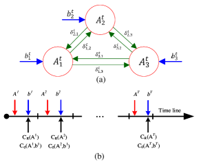
Consider a network of $N$ servers connected by communication links. The system provides access to computing resources for clients. For simplicity, suppose that there is a single type of resource (e.g. memory, CPU, etc.). Denote by $m_{n}$ the total resources available at the $n$-th server. Let $\mathcal{R}_{n}=\{1,\ldots,m_{n}\}$ be the set of possible reservations at the $n$-th server, and $\mathcal{R}=\prod_{n=1}^{N}\mathcal{R}_{n}$ be the set of possible reservations in the entire network. The system operates in discrete time where, at each time slot $t=1,2,\ldots$, the following processes take place chronologically:

  • β€’

    Resource reservation: the network administrator selects the resources $A^{t}=(A^{t}_{1},\ldots,A^{t}_{N})\in\mathcal{R}$ to make available at each server.

  • β€’

    Job requests: the network receives job requests $B^{t}=(B^{t}_{1},\ldots,B^{t}_{N})\in\mathcal{R}$ from its clients to each of its servers.

  • β€’

    Job transfer: the network administrator can shift jobs between the servers to best accommodate the demands.

Let $\delta^{t}_{n,m}$ be the number of jobs transferred from server $n$ to server $m$ at time slot $t$ after receiving the job requests $B^{t}$. These quantities depend on both $A^{t}$ and $B^{t}$, however, this dependency is suppressed to keep the notation simple. Moreover, suppose that the following costs are associated with each of the three processes:

-Reservation cost

given by the function

$\displaystyle C(A^{t})=\sum_{n=1}^{N}f^{R}_{n}(A^{t}_{n}),$

-Violation cost

incurred when the job requests cannot be satisfied

$\displaystyle C_{V}(A^{t},B^{t})=\sum_{n=1}^{N}f^{V}_{n}\big{(}B_{n}^{t}-A_{n}^{t}-\sum_{m=1}^{N}\delta^{t}_{n,m}\big{)},$

-Transfer cost

incurred by the transfer of jobs between the different servers

CT​(At,Bt)=βˆ‘n=1Nβˆ‘mβ‰ nfnT​(Ξ΄n,mt),subscript𝐢𝑇superscript𝐴𝑑superscript𝐡𝑑superscriptsubscript𝑛1𝑁subscriptπ‘šπ‘›subscriptsuperscript𝑓𝑇𝑛subscriptsuperscriptπ›Ώπ‘‘π‘›π‘š\displaystyle C_{T}(A^{t},B^{t})=\sum_{n=1}^{N}\sum_{m\neq n}f^{T}_{n}\big{(}\delta^{t}_{n,m}\big{)},

where $f^{R}_{n},f^{V}_{n},f^{T}_{n}$, for $1\leq n\leq N$, are some positive functions. Therefore, at each time slot $t$, and after receiving the job requests $B^{t}$, the job transfer coefficients $\{\delta^{t}_{n,m},1\leq n\leq N\}$ are solutions to the following offline minimization problem:

{minβˆ‘n=1N(βˆ‘mβ‰ nfTn(Ξ΄tn,m)+fVn(Bntβˆ’Antβˆ’βˆ‘mβ‰ nΞ΄tn,m)),s.t.Β Ξ΄tn,m≀min{(Btnβˆ’Ant)+,(Atmβˆ’Btm)+},βˆ€nβ‰ m.\begin{split}\left\{\begin{tabular}[]{l}$\min\sum\limits_{n=1}^{N}\big{(}\sum\limits_{m\neq n}f^{T}_{n}(\delta^{t}_{n,m})+f^{V}_{n}\big{(}B_{n}^{t}-A_{n}^{t}-\sum\limits_{m\neq n}\delta^{t}_{n,m}\big{)}\big{)},$\\ s.t. $\delta^{t}_{n,m}\leq\min\big{\{}(B^{t}_{n}-A_{n}^{t})^{+},(A^{t}_{m}-B^{t}_{m})^{+}\big{\}},\forall n\neq m$.\end{tabular}\right.\end{split} (1)

One then aims to minimize the reservation cost $C(A^{t})$ while maintaining the sum $C_{0}(A^{t},B^{t}):=C_{V}(A^{t},B^{t})+C_{T}(A^{t},B^{t})$ of the violation and transport costs under a given threshold $v>0$. Nevertheless, since it is an online problem, its optimal solution is out of reach. In particular, one cannot guarantee that the constraint is satisfied. Instead, one aims to solve the following online optimization problem with a long-term constraint over time horizons $T>0$:

{min{At}t=1Tβˆ‘t=1TC(At),s.t.:Β 1Tβˆ‘t=1TC0(At,Bt)≀v,\begin{split}\left\{\begin{tabular}[]{l}$\min\limits_{\{A^{t}\}_{t=1}^{T}}\sum\limits_{t=1}^{T}C(A^{t})$,\\ s.t.: $\frac{1}{T}\sum\limits_{t=1}^{T}C_{0}(A^{t},B^{t})\leq v$,\end{tabular}\right.\end{split} (2)

More precisely, one searches for an online control policy that uses the cumulative information available so far to make the reservations at the next time slot. Again, since the reservation $A^{t}$ is selected before the job request $B^{t}$ is known, we will not be able to reach the optimal solution to (2)2(\ref{opt-pb-on}), but instead, we opt to attain a total reservation cost that is not too large compared to some benchmark that knows the job requests in advance, and meanwhile, to ensure that the constraint is asymptotically satisfied on average over large time horizons. Specifically, we assume the following an ”ideal” optimization problem where the values of job requests $\{B^{t}\}_{t=1}^{T}$ are known in advance for the entire horizon $T$:

{minAβˆˆβ„›βˆ‘t=1TC(A),s.t.βˆ‘s=1tC0(A,Bs)≀v,Β βˆ€t≀T.\begin{split}\left\{\begin{tabular}[]{l}$\min\limits_{A\in\mathcal{R}}\sum\limits_{t=1}^{T}C(A)$,\\ s.t.$\sum\limits_{s=1}^{t}C_{0}(A,B^{s})\leq v$, $\forall t\leq T$.\end{tabular}\right.\end{split} (3)

Denote by $A^{*}$ the optimal static solution to (3)3(\ref{opt-pb-hind-no-rand}). Therefore, the regret of not selecting $A^{*}$ over the horizon $T$ is defined by

$\displaystyle R_{T}=\sum_{t=1}^{T}\big{(}C(A^{t})-C(A^{*})\big{)}.$ (4)

We present in this paper a randomized algorithm that produces a sub-linear regret in time. This corresponds to a time average regret converging towards zero as the time reaches infinity. The intuition behind this is that the algorithm is learning and improves its performance as it accumulates knowledge.

Remark 1

One can consider a different formulation of the problem by minimizing the total cost of reservation, violation, and transfer; see [b24].

Refer to caption
Figure 1: (a) The network model for three nodes at time $t$. (b) The reservation, job requests, and cost calculation timeline.

III Online randomized reservations

Notice that the reservation set $\mathcal{R}$ is discrete. Therefore, the classical gradient type algorithms (see e.g. [b17]) might not be directly applicable since no convexity assumption is possible. To overcome this issue, we introduce randomization in the decision process where, at every time step, the network administrator chooses a probability distribution $P^{t}$ over the set $\mathcal{R}$ of reservations, based on the past job requests, and then draws the reservation $A^{t}$ randomly according to $P^{t}$. Especially, define

$\displaystyle\mathcal{P}(\mathcal{R})=\bigg{\{}P:=(p_{a})_{a\in\mathcal{R}}\in\mathbb{R}^{|\mathcal{R}|}_{+}:\mbox{ $\sum\limits_{a\in\mathcal{R}}p_{a}=1$}\bigg{\}},$

as the space of probability distributions over $\mathcal{R}$. Moreover, define the expected reservation cost as $\mathbb{E}_{P^{t}}[C(A^{t})]=\sum_{a\in\mathcal{R}}p^{t}_{a}C(a)$. Similarly, define the conditional expected transfer and violation costs given that the job request $B^{t}$ are known, respectively, by $\mathbb{E}_{P^{t}}[C_{T}(A^{t},B^{t})]=\sum_{a\in\mathcal{R}}p^{t}_{a}C_{T}(a,B^{t})$ and $\mathbb{E}_{P^{t}}[C_{V}(A^{t},B^{t})]=\sum_{a\in\mathcal{R}}p^{t}_{a}C_{V}(a,B^{t})$. Since the reservations $\{A_{t}\}_{t=1}^{T}$ are generated randomly, the regret is now a random variable. Let us thus introduce the expected regret $\tilde{R}_{T}$ defined in terms of expected costs. More precisely, conditioned on the fact that the values of job request $\{B^{t}\}_{t=1}^{T}$ are known in advance, let the fixed probability distribution $P^{*}=\operatorname*{arg\,min}\limits_{P\in\mathcal{P}(\mathcal{R})}\sum\limits_{t=1}^{T}\mathbb{E}_{P}[C(A^{t})]$ such that $\sum\limits_{s=1}^{t}\mathbb{E}_{P}[C_{0}(A,B^{s})-v]\leq 0,\forall t\leq T$ (in analogy with the fixed allocation $A^{*}$ solution of (3)3(\ref{opt-pb-hind-no-rand})). Then, one defines the expected regret of not playing according to $P^{*}$ over the horizon $T$ as $\tilde{R}_{T}=\sum\limits_{t=1}^{T}\big{(}\mathbb{E}_{P^{t}}[C(A^{t})]-\mathbb{E}_{P^{*}}[C(A^{t})]\big{)}$.

IV Exponentially weighted algorithm with long-time constraints

A classical approach for solving constrained convex optimization problems is the Lagrange multipliers method which consists of finding a saddle point of the Lagrangian function (see, e.g. [b3]). Online versions of these methods have been proposed recently (see, e.g., [b8]).

We propose a different approach by replacing the minimization step in the saddle-point methods with an exponentially weighted step. Our idea is inspired by the exponentially weighted average algorithm introduced in [b10] and [b11], which assigns a weight to each reservation vector based on its past performances. Namely, one wants to perform as well as the best reservation vector. Thus, one weights each reservation vector with a non-increasing function of its past cumulative costs, (cf [b22, Chap. 4.2]). The novelty of the present paper is that it extends the exponentially weighted algorithm to incorporate time-varying constraints. This is done by introducing a step term in the exponent that takes into account the past cumulative constraint violations. In particular, one generates the reservations randomly according to the sequence of probability distributions $\{P^{t}\}_{t\geq 0}$ constructed, at each $t=1,2,\ldots$

$$\begin{split}P^{t}_{a}=\frac{w^{t}(a)}{\sum_{a\in\mathcal{A}}w^{t}(a)},\end{split}$$ (5)

where the weights are given as

wt+1​(a)=exp⁑{βˆ’Ξ·β€‹βˆ‘s=1t(C​(a)+λ​ϝ​(s,a))},superscript𝑀𝑑1π‘Žπœ‚superscriptsubscript𝑠1π‘‘πΆπ‘Žπœ†italic-Οπ‘ π‘Ž\begin{split}w^{t+1}(a)=\exp\bigg{\{}-\eta\sum_{s=1}^{t}\big{(}C(a)+\lambda\digamma(s,a)\big{)}\bigg{\}},\end{split} (6)

with

ϝ​(s,a)=[1sβ€‹βˆ‘r=1s(C0​(a,Br)βˆ’v)]+,italic-Οπ‘ π‘Žsuperscriptdelimited-[]1𝑠superscriptsubscriptπ‘Ÿ1𝑠subscript𝐢0π‘Žsuperscriptπ΅π‘Ÿπ‘£\displaystyle\digamma(s,a)=\bigg{[}\frac{1}{s}\sum_{r=1}^{s}(C_{0}(a,B^{r})-v)\bigg{]}^{+}, (7)

$\eta>0$ a positive parameter, and $B^{1},\ldots,B^{t-1}$ are the values of job requests observed so far. Moreover, $\lambda>0$ can be seen as the analogous of a fixed Lagrange multiplier that calibrates the weight to put on the constraints. Furthermore, we initialize the algorithm with a uniform distribution, i.e. $w^{1}(a)=1$ for all $a\in\mathcal{A}$. Thus, the following recursion is straightforward:

$\displaystyle w^{t+1}(a)=w^{t}(a)\exp\big{\{}-\eta\big{(}C(a)+\lambda\digamma(t,a)\big{)}\big{\}}.$ (8)

The advantage of our approach is twofold. First, one considers the whole history rather than the latest arrival. Steeply, by doing so, one avoids solving minimization problems which can be computationally heavy. We summarize our approach in Algorithm 1. The selection of parameters $\eta$ and $\lambda$ is discussed in Section V. Notice that the time-average cumulative constraint violations function introduced in (7)7(\ref{digamma}) is similar to the one used in [b21] to extend Follow The Regularized Leader algorithm to encompass time-varying constraints.

V Performance analysis

We analyze in this section the performance of Algorithm 1, first in terms of regret, and then in terms of cumulative constraint violations. Define the feasible sets 𝒒t={aβˆˆπ’œ:βˆ‘r=1s(C0​(a,Br))≀v​s,βˆ€s≀t}subscript𝒒𝑑conditional-setπ‘Žπ’œformulae-sequencesuperscriptsubscriptπ‘Ÿ1𝑠subscript𝐢0π‘Žsuperscriptπ΅π‘Ÿπ‘£π‘ for-all𝑠𝑑\mathcal{G}_{t}=\big{\{}a\in\mathcal{A}:\sum_{r=1}^{s}(C_{0}(a,B^{r}))\leq vs,\forall s\leq t\big{\}}, and β„°t={Pβˆˆπ’«β€‹(π’œ):βˆ‘r=1s𝔼P​[C0​(a,Br)]≀v​s,βˆ€s≀t}subscriptℰ𝑑conditional-setπ‘ƒπ’«π’œformulae-sequencesuperscriptsubscriptπ‘Ÿ1𝑠subscript𝔼𝑃delimited-[]subscript𝐢0π‘Žsuperscriptπ΅π‘Ÿπ‘£π‘ for-all𝑠𝑑\mathcal{E}_{t}=\big{\{}P\in\mathcal{P}(\mathcal{A}):\sum_{r=1}^{s}\mathbb{E}_{P}[C_{0}(a,B^{r})]\leq vs,\forall s\leq t\big{\}}. Moreover, we assume the following in the sequel:

  1. 1.

    Cost boundedness: there exists a constant $\Theta>0$ such that, for all $a,b\in\mathcal{R}$,

    $\displaystyle\big{|}C(a)\big{|}\leq\Theta,\big{|}C_{T}(a,b)\big{|}\leq\Theta,\mbox{ and }\big{|}C_{V}(a,b)\big{|}\leq\Theta.$
  2. 2.

    The subspaces $\mathcal{G}_{t}$ and $\mathcal{E}_{t}$ are not empty for all $t\geq 1$.

Algorithm 1 Exponentially weighted method for online reservation with time-varying constraints
  • β€’

    Initialize the values of $P^{0}\in\mathcal{P}(\mathcal{R})$, $B^{0}\in\mathcal{R}$, and $\lambda\geq 0$

  • β€’

    At each step $t=1,2,\ldots$

    • –

      Observe $B^{t-1}$.

    • –

      For each $a\in\mathcal{A}$ compute:

    wt​(a)=exp⁑{βˆ’Ξ·β€‹βˆ‘s=1tβˆ’1(C​(a)+λ​ϝ​(s,a))},superscriptπ‘€π‘‘π‘Žπœ‚superscriptsubscript𝑠1𝑑1πΆπ‘Žπœ†italic-Οπ‘ π‘Ž\begin{split}w^{t}(a)=\exp\bigg{\{}-\eta\sum_{s=1}^{t-1}\big{(}C(a)+\lambda\digamma(s,a)\big{)}\bigg{\}},\end{split}
    $\displaystyle P^{t}_{a}=\frac{w^{t}(a)}{\sum_{a\in\mathcal{A}}w^{t}(a)},$
  • β€’

    Generate $a^{t}$ according to $P^{t}$ and pay the costs

V-A Regret bound

Let $\{P^{t}\}_{t\geq 1}$ be the sequence of probability distribution produced by Algorithm 1 and let $\{A^{t}\}_{t\geq 1}$ be the sequence of corresponding random reservations. Recall that the regret over finite horizons $T>0$, given by the formula (4)4(\ref{reg-rand}), quantifies the difference between the cumulative cost incurred by the exponentially weighted algorithm and the cumulative cost that would have been experienced if the algorithm had possessed perfect information and could have made the best-fixed decisions in hindsight. We show next that the regret is sublinear in $T$ with high probability, regardless of the value of the job request sequence.

Theorem V.1

For any $0<\delta<1$, the regret related to Algorithm 1 satisfies, with a probability at least $1-\delta$,

$$\begin{split}R_{T}&\leq\kappa T+\frac{\log|\mathcal{A}|}{\eta}+\Theta\sqrt{\frac{1}{2}\log(\delta^{-1})T},\end{split}$$ (9)

where $\kappa=\frac{\eta}{8}(1+2\lambda)^{2}\Theta^{2}$. In particular, if $\eta=\frac{1}{\sqrt{T}}$, then $R_{T}=\mathcal{O}(\sqrt{T})$ (sublinear in $T$).

Proof:

First, notice that

$\displaystyle\log\frac{\sum_{a\in\mathcal{A}}w^{t+1}(a)}{\sum_{a\in\mathcal{A}}w^{1}(a)}$ $\displaystyle\geq-\eta\min_{a\in\mathcal{G}_{t}}\sum_{s=1}^{t}C(a)-\log|\mathcal{A}|.$

Moreover,

logβ‘βˆ‘aβˆˆπ’œwt+1​(a)βˆ‘aβˆˆπ’œw1​(a)=βˆ‘s=1tlogβ‘βˆ‘aβˆˆπ’œws+1​(a)βˆ‘aβˆˆπ’œws​(a).subscriptπ‘Žπ’œsuperscript𝑀𝑑1π‘Žsubscriptπ‘Žπ’œsuperscript𝑀1π‘Žsuperscriptsubscript𝑠1𝑑subscriptπ‘Žπ’œsuperscript𝑀𝑠1π‘Žsubscriptπ‘Žπ’œsuperscriptπ‘€π‘ π‘Ž\displaystyle\log\frac{\sum_{a\in\mathcal{A}}w^{t+1}(a)}{\sum_{a\in\mathcal{A}}w^{1}(a)}=\sum_{s=1}^{t}\log\frac{\sum_{a\in\mathcal{A}}w^{s+1}(a)}{\sum_{a\in\mathcal{A}}w^{s}(a)}. (10)

Furthermore, define the random variable $A^{s}$ such that ℙ​(As=a)=ws​(a)βˆ‘aβˆˆπ’œws​(a)β„™superscriptπ΄π‘ π‘Žsuperscriptπ‘€π‘ π‘Žsubscriptπ‘Žπ’œsuperscriptπ‘€π‘ π‘Ž\mathbb{P}(A^{s}=a)=\frac{w^{s}(a)}{\sum_{a\in\mathcal{A}}w^{s}(a)}. Thus, by (8)8(\ref{rec-exp}) one obtains

$\displaystyle\log\frac{\sum_{a\in\mathcal{A}}w^{s+1}(a)}{\sum_{a\in\mathcal{A}}w^{s}(a)}=\log\mathbb{E}_{P^{s}}\big{[}\exp\big{\{}-\eta\big{(}C(a)$
$\displaystyle\qquad\qquad\qquad\qquad\qquad\qquad\qquad+\lambda\digamma(s,a)\big{)}\big{\}}\big{]}.$

Now, by the assumptions above one deduces that C​(a)+λ​ϝ​(s,a)≀(1+2​λ)β€‹Ξ˜πΆπ‘Žπœ†italic-Οπ‘ π‘Ž12πœ†Ξ˜C(a)+\lambda\digamma(s,a)\leq(1+2\lambda)\Theta. Therefore, by Hoeffding’s lemma ([b31, Lemma 2.6]), one gets

logβ‘βˆ‘aβˆˆπ’œws+1​(a)βˆ‘aβˆˆπ’œws​(a)subscriptπ‘Žπ’œsuperscript𝑀𝑠1π‘Žsubscriptπ‘Žπ’œsuperscriptπ‘€π‘ π‘Ž\displaystyle\log\frac{\sum_{a\in\mathcal{A}}w^{s+1}(a)}{\sum_{a\in\mathcal{A}}w^{s}(a)} β‰€βˆ’Ξ·β€‹π”ΌPs​[C​(a)+λ​ϝ​(s,a)]+ΞΊ.absentπœ‚subscript𝔼superscript𝑃𝑠delimited-[]πΆπ‘Žπœ†italic-Οπ‘ π‘Žπœ…\displaystyle\leq-\eta\mathbb{E}_{P^{s}}[C(a)+\lambda\digamma(s,a)]+\kappa.

Thus,

$\displaystyle-\eta\min_{a\in\mathcal{G}_{t}}\sum_{t=1}^{T}C(a)$ $\displaystyle\leq-\eta\sum_{t=1}^{T}\mathbb{E}_{P^{t}}[C(a)+\lambda\digamma(t,a)]$
$\displaystyle\quad+\kappa T+\log|\mathcal{A}|.$

Now, notice that $C(A^{*})=\mathbb{E}_{P^{*}}[C(a)]$, from which we get

$$\begin{split}\sum_{t=1}^{T}\mathbb{E}_{P^{t}}[C(a)+\lambda\digamma(t,a)]&-\mathbb{E}_{P^{*}}[C(A)]\leq\kappa T+\frac{\log|\mathcal{A}|}{\eta}.\end{split}$$

Now, since $\digamma(t,a)\geq 0$ for all $t\geq 0$ one obtains that the expected regret satisfies

$$\begin{split}\tilde{R}_{T}&\leq\kappa T+\frac{\log|\mathcal{A}|}{\eta}.\end{split}$$ (11)

Suppose that the values of job requests are $\{B^{t}\}_{t=1}^{T}=\{b^{t}\}_{t=1}^{T}$. Moreover, let $A^{*}$ be the optimal solution to the following constrained combinatorial optimization problem

$$\begin{split}\min\limits_{A\in\mathcal{G}_{t}}\sum\limits_{t=1}^{T}C_{R}(A),\end{split}$$ (12)

Therefore, the regret of not playing $A^{*}$ over the horizon $T$ is given by

$\displaystyle R_{T}=\sum_{t=1}^{T}\big{(}C_{R}(A^{t})-C(A^{*})\big{)}.$

Define the random variables

$\displaystyle X^{t}=C_{R}(A)-\mathbb{E}_{P^{t}}[C_{R}(A^{t})].$

Then, by the assumption above, $|X^{t}|\leq\Theta$. Therefore, $\{X_{t}\}_{t\geq 1}$ is a sequence of bounded martingales differences, and $Y_{T}=\sum_{t=1}^{T}X_{t}$ is a martingale with respect to the filtration $\mathcal{F}_{T}=\sigma(A^{t},t\leq T)$. Thus, by Hoeffding-Azuma’s inequality [b32] one gets that, for any $0<\delta<1$,

$\displaystyle\mathbb{P}\bigg{(}Y_{T}\leq\sqrt{\frac{1}{2}\log(\delta^{-1})T\Theta^{2}}\bigg{)}\geq 1-\delta.$

Thus, with probability at least $1-\delta$, one has

$\displaystyle\sum_{t=1}^{T}C_{R}(A^{t})\leq\sum_{t=1}^{T}\mathbb{E}_{P^{t}}[C_{R}(A^{t})]+\sqrt{\frac{1}{2}\log(\delta^{-1})T\Theta^{2}}.$

Now, define the probability distribution $P_{*}\in\mathcal{P}(\mathcal{A})$ as the optimal solution to the following optimization problem

$$\begin{split}\min\limits_{P\in\mathcal{E}_{t}}\sum\limits_{t=1}^{T}\mathbb{E}_{P}[C_{R}(A)]\end{split}$$ (13)

if the values of job requests $\{B^{t}\}_{t=1}^{T}=\{b^{t}\}_{t=1}^{T}$ were known is advance. Then, since $\delta_{A^{*}}\in\mathcal{E}_{t}$, $\sum_{t=1}^{T}\mathbb{E}_{P^{*}}[C_{R}(A)]\leq\sum_{t=1}^{T}C_{R}(A^{*})$. Therefore,

$$\begin{split}R_{T}&\leq\sum_{s=1}^{t}\mathbb{E}_{P^{s}}[C_{R}(A^{s})]-\inf_{P\in\mathcal{E}_{t}}\sum_{s=1}^{t}\mathbb{E}_{P}[C_{R}(A)]\\ &\qquad\qquad+\Theta\sqrt{\frac{1}{2}\log(\delta^{-1})T}.\end{split}$$ (14)

Using (11)11(\ref{exp-reg-bound}) gives (9). $\Box$

V-B Violation constraint bound

We analyze next the expected cumulative time average of the constraint violations.

Theorem V.2

The sequence $\{P^{t}\}_{t=1}^{T}$ produced by Algorithm 1 satisfies:

$$\begin{split}\frac{1}{T}\sum_{t=1}^{T}\mathbb{E}_{P^{t}}[\digamma(t,a)]&\leq\frac{1}{\lambda}\min_{a\in\mathcal{G}_{t}}C(a)+\frac{\log|\mathcal{A}|}{T\lambda\eta}+\frac{1}{\lambda}\kappa.\end{split}$$ (15)

In particular, if $\eta=\frac{1}{\sqrt{T}}$, $\lambda=o(T^{1/4})$ then

$\displaystyle\lim_{T\rightarrow\infty}\frac{1}{T}\sum_{t=1}^{T}\mathbb{E}_{P^{t}}[\digamma(t,a)]\rightarrow 0.$ (16)