Improved Communication-Privacy Trade-offs in Mean Estimation under Streaming Differential Privacy
Abstract
We study mean estimation under central differential privacy and communication constraints, and address two key challenges: firstly, existing mean estimation schemes that simultaneously handle both constraints are usually optimized for geometry and rely on random rotation or Kashin’s representation to adapt to geometry, resulting in suboptimal leading constants in mean square errors (MSEs); secondly, schemes achieving order-optimal communication-privacy trade-offs do not extend seamlessly to streaming differential privacy (DP) settings (e.g., tree aggregation or matrix factorization), rendering them incompatible with DP-FTRL type optimizers. In this work, we tackle these issues by introducing a novel privacy accounting method for the sparsified Gaussian mechanism that incorporates the randomness inherent in sparsification into the DP noise. Unlike previous approaches, our accounting algorithm directly operates in geometry, yielding MSEs that fast converge to those of the uncompressed Gaussian mechanism. Additionally, we extend the sparsification scheme to the matrix factorization framework under streaming DP and provide a precise accountant tailored for DP-FTRL type optimizers. Empirically, our method demonstrates at least a 100x improvement of compression for DP-SGD across various FL tasks.
1 Introduction
In federated learning (FL) (McMahan et al., 2016; Konečnỳ et al., 2016; Kairouz et al., 2021c), a server executes a specific learning task on data that is kept on clients’ devices, avoiding the explicit collection of local raw datasets. This process typically involves the server iteratively gathering essential local model updates (such as noisy gradients) from the client side and subsequently updating the global model. While FL embodies the principle of data minimization by only requesting the minimal information necessary for model training, these local model updates may still contain sensitive information. As a result, additional privacy protection is necessary to prevent the trained model from possibly revealing individual information. Moreover, with the increase of model size, the exchange of local model updates becomes both memory and computation-intensive, leading to substantial latency and impeding the efficiency of training cycles. Consequently, it is desired to devise robust privacy protection mechanisms that simultaneously optimize communication efficiency.
In this paper, we study the mean estimation111Here, refers to the geometry of the local model updates, i.e., for all client . This condition is typically maintained through the clipping step of the differential privacy mechanism., a core sub-routine in the majority of FL schemes, subject to joint communication and differential privacy (DP) (Dwork et al., 2006) constraints. We consider two major types of DP optimization settings: (1) the classic DP-SGD type approach (Abadi et al., 2016) where independent DP noise is injected in each round of training, and (2) the DP-FTRL type approach (Guha Thakurta and Smith, 2013; Kairouz et al., 2021b; Denisov et al., 2022) where the DP noise is correlated across training rounds, the structure of which is intricately designed based on certain matrix factorization.
There has been a long thread of literature on distributed mean estimation (DME) under either or both privacy and communication constraints (Suresh et al., 2017; Konečnỳ et al., 2016; Agarwal et al., 2018; Chen et al., 2020, 2023; Shah et al., 2022; Feldman and Talwar, 2021; Isik et al., 2023a; Asi et al., 2023). Recent work by Chen et al. (2023) points out that, to achieve order-optimal mean square errors (MSEs) under joint constraints, it becomes imperative to integrate the inherent randomness utilized in compression (e.g., in sampling, sketching, or projection) into privacy analysis. Essentially, the implicit “compression noise” should be leveraged to amplify the DP guarantees, resulting in a significant reduction of DP noise. However, despite the coordinate subsampled Gaussian mechanism (CSGM) introduced by Chen et al. (2023) achieving order-optimal MSEs, it is crafted within the geometry (i.e., assuming for any local vector ) and relies on random rotation or Kashin’s representation to extend to mean estimation tasks. It is noteworthy that the bounded norm assumption is strictly more robust than the bounded norm assumption (see Section 4.2), inevitably leading to larger MSEs with CSGM compared to the (uncompressed) Gaussian mechanism under equivalent DP guarantees.
A further challenge arises in CSGM (or, more broadly, general randomized compression schemes based on random projection, sampling, or sketching) when applied to streaming DP models (Guha Thakurta and Smith, 2013; Denisov et al., 2022; Jain et al., 2023), particularly in the context of DP-FTRL type optimization mechanisms based on tree aggregation (Honaker, 2015; Kairouz et al., 2021b) or matrix factorization (Denisov et al., 2022). In the streaming DP model, the DP noise injected in each round loses its independence. Instead, noise variables are correlated across training rounds through a linear transform , where is obtained from certain matrix factorization of the objective function that aims to minimize the overall distortions, such as MSEs. When the noise variables are correlated across rounds, they are no longer “aligned” with the randomness introduced in the local compression phase, as compression occurs locally and is thus independent across rounds. This complicates the analysis of privacy amplification, as privacy budgets cannot be accounted for round-wise, introducing what we term “temporal coupling.” Moreover, the adaptive nature of DP-FTRL, where local gradients depend on the outputs of previous rounds, leads to the coupling of compression seeds that are typically introduced independently across dimensions. When analyzing the outputs over rounds, this coupling, referred to as “spatial coupling,” presents a significant challenge. Traditional privacy amplification tools (Balle et al., 2018; Zhu and Wang, 2019; Wang et al., 2019) fail in the face of such spatial and temporal coupling, necessitating a novel analysis approach.
Our contribution.
In this work, we tackle both aforementioned challenges. Firstly, we introduce a novel privacy accounting method for the sparsified Gaussian mechanism. This method incorporates the inherent randomness from the sparsification phase into the DP noise. Unlike previous approaches in Chen et al. (2023), our accounting algorithm directly operates in geometry, resulting MSEs that converge fast to those of the uncompressed Gaussian mechanism. The key technique is to leverage the convexity of the Rényi DP profile of -dimensional subsampled Gaussian mechanism and extend it to multi-dimensional scenarios.
Secondly, we extend the application of the sparsified Gaussian mechanism to streaming DP settings, particularly within the matrix factorization DP-FTRL framework. We establish a Rényi privacy accounting theorem. While this theorem bears similarities to its non-streaming counterpart, the analysis necessitates a fundamentally different approach due to the spatial and temporal coupling inherent in the adaptive releases. A crucial step in our analysis involves decomposing the transcript (i.e., the collection of all releases across training rounds), effectively transforming the adaptive releasing model into a non-adaptive one.
Although our analysis primarily revolves around the sparsified Gaussian mechanism (or coordinate subsampled Gaussian mechanism), it inherently encompasses a broader family of random projections, including subsampled randomized Hadamard transform (Ailon and Chazelle, 2006; Sarlos, 2006), and randomized Gaussian design (Wainwright, 2019, Section 6). These dimensionality reduction techniques can be viewed as a linear transform followed by a subsampling step. Additionally, by slightly lifting the dimension, these random designs exhibit deep connections to Kashin’s representation, providing a uniform bound, albeit with a larger leading constant (Lyubarskii and Vershynin, 2010).
Finally, we present comprehensive empirical results on the proposed sparsified Gaussian mechanism and sparsified Gaussian matrix factorization. Our results demonstrate a improvement in compression rates in various FL tasks (including FMNIST and Stackoverflow datasets). Moreover, our algorithm reduces the dimensionality of local model updates and hence can potentially be combined with other quantization or (scalar) lossless compression techniques (Alistarh et al., 2017; Isik et al., 2022; Mitchell et al., 2022).
2 Related Work
FL and DME. Federated learning (Konečnỳ et al., 2016; McMahan et al., 2016; Kairouz et al., 2019) emerges as a decentralized machine learning framework that provides data confidentiality by retaining clients’ raw data on edge devices. In FL, communication between clients and the central server can quickly become a bottleneck (McMahan et al., 2016), so previous works have focused on compressing local model updates via gradient quantization (McMahan et al., 2016; Alistarh et al., 2017; Gandikota et al., 2019; Suresh et al., 2017; Wen et al., 2017; Wangni et al., 2018; Braverman et al., 2016), sparsification (Barnes et al., 2020; Hu et al., 2021; Farokhi, 2021; Isik et al., 2023b; Lin et al., 2018), or random projection (Rothchild et al., 2020; Vargaftik et al., 2021). To further enhance user privacy, FL is often combined with differential privacy (Dwork et al., 2006; Abadi et al., 2016; Agarwal et al., 2018; Hu et al., 2021).
Note that in this work, we consider FL (or more specifically, DME) under a central-DP setting where the server is trusted, which is different from the local DP model (Kasiviswanathan et al., 2011)222Another alternative to private DME is via local DP and shuffling. We provide a detailed discussion on this direction in Appendix B and the distributed DP model with secure aggregation (Bonawitz et al., 2016; Bell et al., 2020; Kairouz et al., 2021a; Agarwal et al., 2021; Chen et al., 2022b, a). When the secure aggregation is employed, local model updates cannot be compressed independently (Rothchild et al., 2020; Chen et al., 2023), and hence, the corresponding compression rates must be strictly higher than those without secure aggregation.
Streaming DP and DP-FTRL. In addition to the classic DP optimizers such as DP-SGD (Abadi et al., 2016) or DP-FedAvg (McMahan et al., 2016), we also study the online optimization settings such as DP-FTRL (Kairouz et al., 2021b) where the noise is correlated across rounds. This is motivated by the facts that (1) subsampling is often impractical in federated learning settings (Kairouz et al., 2021b, 2019), and (2) the correlated noise probably yields better utility compared to the independent noise (Choquette-Choo et al., 2023a). The key component behind the DP-FTRL relies on the private releases under continual observation, an old problem dating back to (Dwork et al., 2010; Chan et al., 2012). Since then, several works have studied the continual release model and its applications (Upadhyay and Upadhyay, 2021; Choquette-Choo et al., 2022, 2023a; Henzinger et al., 2023, 2024). Kairouz et al. (2021b) originally used the efficient DP binary-tree estimator (Honaker, 2015) for the DP-FTRL algorithm, but later, a more general approach to cumulative sums based on matrix factorization (Hardt and Talwar, 2010; Li et al., 2015; Yuan et al., 2016; McKenna et al., 2018; Edmonds et al., 2020) was used. We, however, note that DP online optimization concerns adaptive inputs, that is, the future data points depend on previous outputs, and not all matrix mechanisms extend to the adaptive settings (Denisov et al., 2022), and it introduces challenges when incorporating compression into the privacy analysis. Indeed, to prove the adaptive DP guarantees of our algorithm, we need to handle the spatial and temporal dependency carefully. Finally, while the recent work Choquette-Choo et al. (2023b) also investigate privacy amplification through subsampling, their subsampling is conducted client-wise rather than coordinate-wise, as their scheme is not designed for compression. Consequently, Choquette-Choo et al. (2023b) do not encounter the spatial coupling issue as we do.
3 Preliminaries and Setups
In this section, we introduce the mathematical formulation of the problem and the DP models. We begin with DME in non-streaming DP, and then transition to the continual sum (or mean) problem within the streaming DP model.
3.1 DME and (Non-streaming) DP
Consider clients, each with a local vector (e.g., local gradient or model update) that satisfies for some constant (one can think of as a clipped local gradient). A server aims to learn an estimate of the mean from after communicating with the clients. Toward this end, each client locally compresses into a -bit message through a local encoder (where ) and sends it to the central server, which upon receiving computes an estimate that satisfies the following differential privacy:
Definition 3.1 (Differential Privacy (Dwork et al., 2006))
A mechanism (i.e., a randomized mapping) is -DP if for any neighboring datasets , , and measurable , it holds that
where the probability is taken over the randomness of .
Our goal is to design schemes that minimize the MSE:
subject to -bit communication and -DP constraints.
The above DME task is closely related to FL with batched SGD (or other similar stochastic optimization methods, such as FedAvg (McMahan et al., 2016)). In each round, the server updates the global model using a noisy mean of local model updates. This estimate is typically derived through a DME primitive. As demonstrated in (Ghadimi and Lan, 2013), if the estimate remains unbiased in each round, convergence rates depend on the estimation error. Note that the DME procedure is invoked independently in each round, and the privacy budget is allocated for rounds of training, differing from the online DP setting discussed below.
3.2 Streaming Differential Privacy
Next, we introduce the streaming DME problem and matrix mechanisms. To begin with, we first summarize the streaming DP setting (Denisov et al., 2022). A streaming mechanism takes inputs and outputs at time . We denote the stream with rounds in the following matrix form:
and similarly for and the adversary’s view .
An adversary that adaptively defines two input sequences and . The adversary must satisfy the promise that these sequences correspond to neighboring data sets. The privacy game proceeds in rounds. At round , the adversary generates and , as a function of . The game accepts these if the input streams defined so far are valid, meaning that there exist completions and such that and are neighboring, in the following sense:
Definition 3.2 (Neighboring datasets)
Two data streams and in will be considered to be neighboring if they differ by a single row, with the -norm of the difference in this row at most .
The game is parameterized by a bit , which is unknown to the adversary but constant throughout the game. The game hands either or to , depending on . We say is Rényi DP if the adversary’s views under and is -indistinguishable under Rényi divergence at order :
3.3 DME and Matrix Mechanisms
Finally, we consider DME under the streaming DP model. In each round , the server selects a batch of clients and computes the empirical mean of their local vectors . Note that can depend on previous outputs . Our scheme assumes single-participation-per-epoch, that is, disjoint with .
The goal of matrix mechanisms is to continually release a differentially private version of while minimizing the overall MSE: . Here, must be a lower triangular matrix in order to ensure causality. In online optimization, the matrix is determined by update rules. For instance, in simple SGD with a fixed step size , the model is updated as follows:
resulting in the corresponding being the prefix-sum matrix satisfying . In general, one can leverage the matrix mechanism within the DP-FTRL framework (Kairouz et al., 2021b, Algorithm 1) and further incorporate momentum (Denisov et al., 2022).
To ensure privacy, instead of directly privatizing data matrix (which results in a DP-SGD type scheme), we leverage the factorization for . If -DP is preserved for , then the same level of DP holds for as well. Notbaly, in the online optimization setting, local vectors are adaptively generated and depend on . Denisov et al. (2022, Theorem 2.1) shows that for Gaussian mechanism (i.e., for some ), the non-adaptive DP guarantee (meaning that is independent with the previous private outputs ) implies the same level of adaptive DP.
To optimize the error, Li et al. (2015); Yuan et al. (2016); Denisov et al. (2022) formulate the factorization as a convex optimization problem :
| (1) |
where is the sensitivity of . In this work, while we plug in the optimal factorization in our scheme (specifically solved via the fixed point method in Denisov et al. (2022)), our results hold for general factorization.
Our objective is to devise a local compression mechanism satisfying two criteria: (1) satisfies adaptive streaming DP, and (2) is a function of locally compressed vectors that can be described in bits.
Remark 3.3
In the streaming scenario, the cohort size solely impacts the sensitivity of the mean function each round. For simplicity in privacy analysis, we assume (non-batched SGD). Nevertheless, our results extend to general batch sizes, as outlined in the main theorems.
Notation.
In the non-streaming setting, we employ (or ) to represent the local (row) vector at client . In the streaming scenario, (or ) denotes the averaged row vectors of clients at round . Matrices are denoted by capital bold-faced symbols; for instance, represents the matrix form of the stream , where the -th row of is . When the context is clear, we may use to refer to the stream itself. Additionally, we use or interchangeably to indicate the -th entry of , with and 333In general, we use as the time index, as the coordinate (spatial) index, and as the client index for subscripts and superscripts..
4 Differentially Private Mean Estimation
In this section, we consider the non-streaming DME problem described in Section 3.1. To reduce communication costs under central DP, previous work of Chen et al. (2023) proposes coordinate-subsampled Gaussian mechanism (CSGM), which random sparsifies each local vector in a coordinate-wise fashion, followed by server aggregation and the addition of Gaussian noise. While aligning with several gradient compression techniques, CSGM significantly enhances privacy guarantees by incorporating the randomness introduced in the sparsification phase into privacy analysis.
However, a notable drawback in Chen et al. (2023) emerges within the geometry assumption that requires . It is crucial to note that, in general, the assumption is weaker than the assumption described in Section 3.1. To extend to the scenario, Chen et al. (2023) employs random rotation (or Kashin’s representation) and clipping to pre-process local vectors. This approach, however, results in larger Mean Squared Errors (MSEs) compared to the uncompressed Gaussian mechanism under equivalent Differential Privacy (DP) guarantees.
To address the geometry issue in Chen et al. (2023), we introduce a slight modification (see Algorithm 1) to the CSGM scheme and present an enhanced analysis of its Rényi DP profile, yielding a significantly improved guarantee. To differentiate between the two schemes, we term our proposed version as -CSGM, while the original one in Chen et al. (2023) is referred to as -CSGM. Our main result in this section is the following privacy upper bound for the -CSGM mean estimation scheme.
Theorem 4.1
Let (i.e., ), and for all . Let be defined as in (2) with , and . Then satisfies -Rényi DP, for all integer and
| (3) |
While -CSGM also employs clipping, we do not account for privacy budgets directly based on the clipping norm (which is the case in -CSGM). Instead, we consider both and , with serving to “mitigate” the regime on which the privacy amplification lemma operates. In -CSGM, the clipping norm only influences higher-order terms in the final guarantees, and a slight increase in does not alter the privacy guarantee asymptotically with increasing dimension . In the subsequent subsection, we demonstrate that, for any and under the same MSE constraint, the Rényi DP guarantee of -CSGM converges to that of the (uncompressed) Gaussian mechanism as .
4.1 Compared to the Gaussian Mechanism
We begin with the following lemma that computes the MSE of .
Corollary 4.2
On the other hand, the MSE of the (uncompressed) Gaussian mechanism is . It can be shown that under the same MSE constraints, the Renyi DP of -CSGM converges to that of the Gaussian mechanism in the following sense:
Lemma 4.3
For any fixed sparsification rate and Renyi DP order , let and be chosen such that , i.e., . Then, it holds that as , where is the Rényi DP bound of the Gaussian mechanism, and is defined in (4.1).
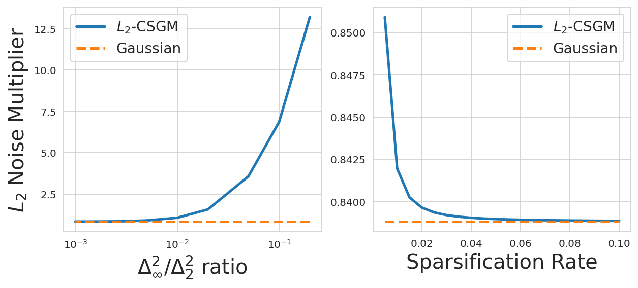
It is worth noting that, in general, the ratio decreases rapidly as increases, leading to as . For instance, by utilizing random rotation for preprocessing local vectors, with high probability, . If further employing Kashin’s representation (Lyubarskii and Vershynin, 2010), then with probability .
On the other hand, if we calibrate the noise based on as in -CGSM, the constant in Rényi DP will not match that of the uncompressed Gaussian mechanism, which we elaborate on in the next subsection.
4.2 Compared to -CSGM (Chen et al., 2023).
To compare the and -CSGM, first observe that the Rényi DP bound in (4.1) can be expressed as
where and . On the other hand, the Rényi DP bound of -CSGM in Chen et al. (2023) is
As a result, the ratio between two Rényi DP bounds is (because implies ). When employing random rotation, this ratio is with high probability; with Kashin’s representation, this ratio remains constant, but the constant is non-negligible (for instance, in Chen et al. (2020), the constant is set to be around ). The sub-optimality gap between -CSGM and the (uncompressed) Gaussian mechanism makes it undesirable in practical FL tasks, emphasizing the necessity of -CSGM.
5 Matrix Factorization Mechanism with Local Sparsification under Streaming DP
Moving on, we delve into the streaming DP setting, specifically focusing on the matrix mechanism detailed in Section 3.2 and Section 3.3.
In the context of matrix mechanisms, the objective is to continually release a DP version of , where each row of may depend on previous outputs . To minimize the overall MSE, , we factorize into and designing DP mechanisms according to , as discussed in Section 3.3. Notably, our scheme adopts the optimal factorization for the prefix sum matrix, addressing the optimization problem (1).
We aim to devise a matrix factorization scheme that simultaneously compresses local gradients . In this approach, instead of transmitting to the server, clients send , with compression applied row-wise (i.e., client-wise). A tempting strategy is to employ the local sparsification technique in CSGM and enhance privacy using Theorem 4.1444Throughout this section, we assume a cohort size of for simplicity. Our results naturally extend to general scenarios, and the full scheme is presented in Algorithm 3 in Appendix A, in which each client adopts an independent sampling mask.: where is a factorization, and for and . However, the privacy analysis encounters two challenges:
-
•
In matrix mechanisms, a local vector may persist across all rounds. Consequently, the randomness introduced in local sparsification steps at the -th round might affect other rounds, resulting in what we term as temporal coupling. Unlike in Denisov et al. (2022), where the temporal coupling of isotropic Gaussian noise can be circumvented due to rotational invariance, local sparsification or sampling breaks this invariance, rendering Theorem 2.1 of Denisov et al. (2022) inapplicable.
-
•
In the streaming scenario, the sampling variable for the -th coordinate in the -round may influence the -th coordinate later due to adaptivity. For instance, can depend on the -th output , which, in turn, is a function of for all . This introduces “spatial correlation,” which does not appear in the non-streaming setting (e.g., Theorem 4.1).
In this section, we demonstrate that despite both temporal and spatial couplings, we can still achieve the same “amplification effect” as in Theorem 4.1. Our primary result is the Rényi Differential Privacy (DP) bound for the sparsified Gaussian matrix factorization outlined in Algorithm 2 (which can be seen as a direct extension of -CSGM to the streaming DP setting).
Theorem 5.1
Let be a lower-triangular full-rank query matrix, and let be any factorization for some , with . Let be the data matrix and and be the and norm bounds of , i.e., and (recall that denotes the -th row of ). Then, the in Algorithm 2 satisfies adaptive -Rényi DP for any and
| (4) |
where and are the and sensitivities.
A couple of remarks follow. Firstly, the class of matrix mechanisms encompasses tree-based methods as a special case, such as or - tree aggregation (Honaker, 2015) used in Kairouz et al. (2021b). Therefore, Theorem 5.1 also applies to these results. Second, while Choquette-Choo et al. (2023b) also investigate privacy amplification through subsampling, their subsampling is conducted client-wise rather than coordinate-wise, as their scheme does not aim for compression. Consequently, Choquette-Choo et al. (2023b) do not encounter the spatial coupling issue. Finally, our scheme assumes single participation per epoch, and in practice, this can be done by shuffling and restarting the mechanism each epoch, similar to the TreeRestart approach in Kairouz et al. (2021b).
5.1 Proof of Theorem 5.1
Next, we prove Theorem 5.1. The proof begins with the LQ decomposition trick in Denisov et al. (2022), followed by a careful decoupling of the joint distribution on .
Reparameterization.
Let be the LQ decomposition of the matrix . Consider a different lower-triangular factorization: where , is orthonormal, and both and are lower-triangular. Since is lower-triangular, can operate in the continuous release model, as row of depends only on the first rows of . Following from the same argument in Denisov et al. (2022, Theorem 2.1), it suffices to show the desired DP guarantee (5.1) on since we can always replace with due to the rotational invariance of isotropic Gaussian distribution. For notational convenience, we denote in the remaining proof (note that is lower triangular).
Joint density of the transcript.
Next, we show the mechanism is an instance of the standard (subsampled) Gaussian mechanism for computing an adaptive function in the continuous release model with a guaranteed bound on the global and sensitivities. Let and be any two neighboring data streams (defined in Definition 3.2) that additionally satisfy the following condition: . Without loss of generality, we assume that and differ at , and thus when analyzing the privacy guarantees, we condition on the realization and all the potential randomness used in the optimization algorithm, treating them as deterministic. The only randomness that will be accounted for in the privacy analysis is and .
Given the data stream , the output transcript is computed as follows:
for all . Our goal is to control where denotes the distribution of transcript under data stream and denotes the distribution of under . Note that the randomness used to compute the above divergence only includes and , as we have conditioned on all other (irrelevant) external randomness, including .
Decoupling the joint distribution.
The main challenge here, compared to the uncompressed Gaussian mechanism in Denisov et al. (2022), is the spatial and temporal coupling on the joint distribution . To see this, observe that implicitly depends on the -th sampling variable through (which are functions of ). As a result, the joint distribution of is a mixture of product distributions, so the scheme cannot be reduced into a simple subsampled Gaussian mechanism.
To address this issue, we introduce the following decomposition trick on the transcript to decouple the complicated spatial and temporal correlation. For all , write , , and
so that .
The key observation is that, conditioned on the realization , is a deterministic function of . To see this, note that
for some functions and . Also notice that . Thus, by induction, is a function of .
As a result, the overall transcript can be viewed as a post-processing of , so by data processing inequality, it holds that
| (5) |
Since the does not have spatial coupling, in the sense that is independent of for all and , , we can invoke the argument of Denisov et al. (2022) along with privacy amplification by subsampling, summarized as in the following lemma.
Lemma 5.2
Let be defined as above. Then, it holds that
We remark that (5) implies that among all possible adaptive dependencies of , the transcript is statistically dominated by the independent one, that is, remains constant regardless of previous outputs .
6 Empirical Evaluation
We provide empirical evaluations on the privacy-utility trade-offs for both DP-SGD (under a non-streaming setting) and DP-FTRL type (with matrix mechanisms Denisov et al. (2022)) algorithms. We mainly compare the -CGSM (Algorithm 2) and sparsified Gaussian matrix factorization (Algorithm 2) with the uncompressed Gaussian mechanism (Balle and Wang, 2018). We convert the Rényi DP bounds to -DP via the conversion lemma from Canonne et al. (2020) for a fair comparison.
Datasets and models. We run experiments on the full Federated EMNIST (Cohen et al., 2017) and Stack Overflow (Authors., 2019) dataset. F-EMNIST has classes and clients with a total of training samples. Inputs are single-channel images. The Stack Overflow (SO) dataset is a large-scale text dataset based on responses to questions asked on the site Stack Overflow. There are over data samples unevenly distributed across clients. We focus on the next word prediction (NWP) task: given a sequence of words, predict the next words in the sequence.
On F-EMNIST, we experiment with a (4 layer) Convolutional Neural Network (CNN) used by Kairouz et al. (2021a) (with around million parameters). On SONWP, we experiment with a million parameters ( layer) long-short term memory (LSTM) model – the same as prior work Andrew et al. (2021); Kairouz et al. (2021a). In both cases, clients train for local epoch using SGD. Only the server uses momentum.
Additionally, for local model updates, we perform random rotation and -clipping, with , where is the model dimension (i.e., trainable parameters) and is the cohort size in each training round.
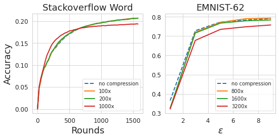
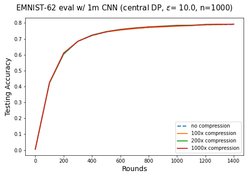
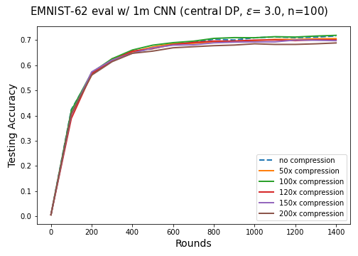
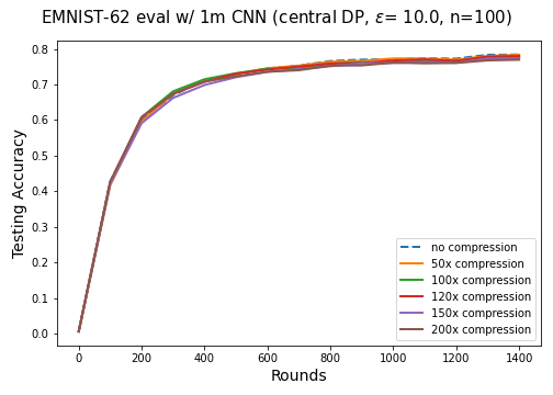
-CSGM for DP-SGD.
In Figure 2, we report the accuracy of -CSGM (Algorithm 1) as well as the uncompressed Gaussian mechanism.
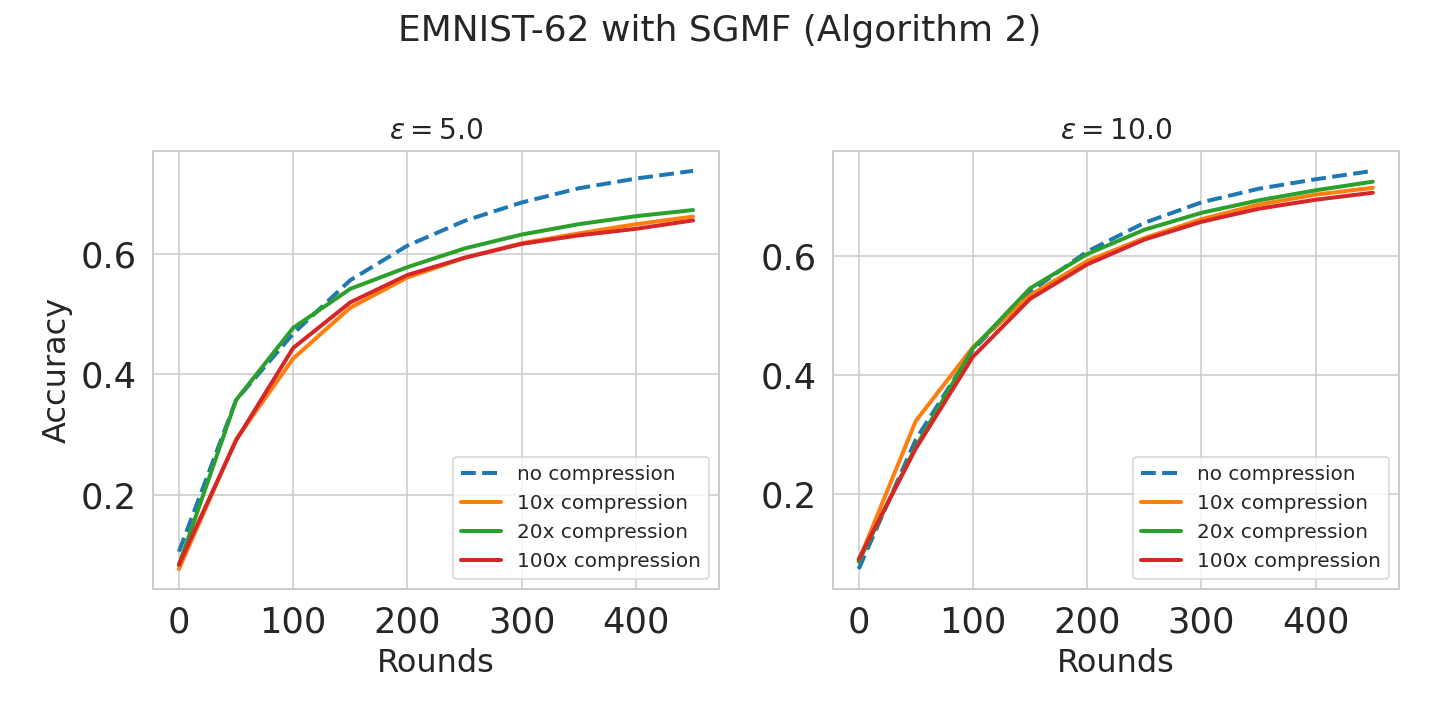
Sparsified Gaussian Matrix Mechanism for DP-FTRL. In Figure 3, we report the accuracy of SGMF (Algorithm 1) and the uncompressed matrix mechanism. We use the same optimal factorization as in Denisov et al. (2022) with for 16 epochs, and we restart the mechanism and shuffling clients every epoch as in the approach in Kairouz et al. (2021b). We observe that for the matrix mechanism, the compression rates are, in general, less than DP-FedAvg, and in addition, the performance is more sensitive to server learning rates and clip norms.
7 Conclusion
Our work addresses challenges in mean estimation under central DP and communication constraints. We introduce a novel Rényi DP accounting algorithm for the sparsified Gaussian mechanism that significantly improves upon previous ones based on sensitivity. We also extend the scheme and accountant to the streaming setting, providing an adaptive DP bound that handles spatial and temporal couplings of privacy loss unique to adaptive settings. Empirical evaluations on diverse federated learning tasks showcase a 100x enhancement in compression. Notably, our scheme focuses on reducing the dimensionality of local model updates, and hence it can potentially be combined with other gradient quantization or compression techniques, thereby promising heightened compression efficiency.
References
- Abadi et al. (2016) Martin Abadi, Andy Chu, Ian Goodfellow, H Brendan McMahan, Ilya Mironov, Kunal Talwar, and Li Zhang. Deep learning with differential privacy. In Proceedings of the 2016 ACM SIGSAC conference on computer and communications security, pages 308–318, 2016.
- Agarwal et al. (2018) Naman Agarwal, Ananda Theertha Suresh, Felix Xinnan X Yu, Sanjiv Kumar, and Brendan McMahan. cpSGD: Communication-efficient and differentially-private distributed sgd. In Advances in Neural Information Processing Systems, pages 7564–7575, 2018.
- Agarwal et al. (2021) Naman Agarwal, Peter Kairouz, and Ziyu Liu. The Skellam mechanism for differentially private federated learning. Advances in Neural Information Processing Systems, 34:5052–5064, 2021.
- Ailon and Chazelle (2006) Nir Ailon and Bernard Chazelle. Approximate nearest neighbors and the fast johnson-lindenstrauss transform. In Proceedings of the thirty-eighth annual ACM symposium on Theory of computing, pages 557–563, 2006.
- Alistarh et al. (2017) Dan Alistarh, Demjan Grubic, Jerry Li, Ryota Tomioka, and Milan Vojnovic. QSGD: Communication-efficient sgd via gradient quantization and encoding. In Advances in Neural Information Processing Systems 30, pages 1709–1720, 2017.
- Andrew et al. (2021) Galen Andrew, Om Thakkar, Brendan McMahan, and Swaroop Ramaswamy. Differentially private learning with adaptive clipping. Advances in Neural Information Processing Systems, 34:17455–17466, 2021.
- Asi et al. (2022) Hilal Asi, Vitaly Feldman, and Kunal Talwar. Optimal algorithms for mean estimation under local differential privacy. In International Conference on Machine Learning, pages 1046–1056. PMLR, 2022.
- Asi et al. (2023) Hilal Asi, Vitaly Feldman, Jelani Nelson, Huy Nguyen, and Kunal Talwar. Fast optimal locally private mean estimation via random projections. In Thirty-seventh Conference on Neural Information Processing Systems, 2023. URL https://openreview.net/forum?id=K3JgUvDSYX.
- Authors. (2019) The TensorFlow Federated Authors. Tensorflow federated stack overflow dataset, 2019.
- Balle and Wang (2018) Borja Balle and Yu-Xiang Wang. Improving the gaussian mechanism for differential privacy: Analytical calibration and optimal denoising. In International Conference on Machine Learning, pages 394–403. PMLR, 2018.
- Balle et al. (2018) Borja Balle, Gilles Barthe, and Marco Gaboardi. Privacy amplification by subsampling: Tight analyses via couplings and divergences. Advances in Neural Information Processing Systems, 31, 2018.
- Barnes et al. (2020) Leighton Pate Barnes, Huseyin A Inan, Berivan Isik, and Ayfer Özgür. rtop-k: A statistical estimation approach to distributed sgd. IEEE Journal on Selected Areas in Information Theory, 1(3):897–907, 2020.
- Bell et al. (2020) James Henry Bell, Kallista A Bonawitz, Adrià Gascón, Tancrède Lepoint, and Mariana Raykova. Secure single-server aggregation with (poly) logarithmic overhead. In Proceedings of the 2020 ACM SIGSAC Conference on Computer and Communications Security, pages 1253–1269, 2020.
- Bhowmick et al. (2018) Abhishek Bhowmick, John Duchi, Julien Freudiger, Gaurav Kapoor, and Ryan Rogers. Protection against reconstruction and its applications in private federated learning. arXiv preprint arXiv:1812.00984, 2018.
- Bonawitz et al. (2016) Keith Bonawitz, Vladimir Ivanov, Ben Kreuter, Antonio Marcedone, H Brendan McMahan, Sarvar Patel, Daniel Ramage, Aaron Segal, and Karn Seth. Practical secure aggregation for federated learning on user-held data. arXiv preprint arXiv:1611.04482, 2016.
- Braverman et al. (2016) Mark Braverman, Ankit Garg, Tengyu Ma, Huy L Nguyen, and David P Woodruff. Communication lower bounds for statistical estimation problems via a distributed data processing inequality. In Proceedings of the forty-eighth annual ACM Symposium on Theory of Computing, pages 1011–1020, 2016.
- Canonne et al. (2020) Clément L Canonne, Gautam Kamath, and Thomas Steinke. The discrete gaussian for differential privacy. arXiv preprint arXiv:2004.00010, 2020.
- Chan et al. (2012) T H Hubert Chan, Mingfei Li, Elaine Shi, and Wenchang Xu. Differentially private continual monitoring of heavy hitters from distributed streams. In Privacy Enhancing Technologies: 12th International Symposium, PETS 2012, Vigo, Spain, July 11-13, 2012. Proceedings 12, pages 140–159. Springer, 2012.
- Chen et al. (2020) Wei-Ning Chen, Peter Kairouz, and Ayfer Ozgur. Breaking the communication-privacy-accuracy trilemma. Advances in Neural Information Processing Systems, 33, 2020.
- Chen et al. (2022a) Wei-Ning Chen, Christopher A Choquette Choo, Peter Kairouz, and Ananda Theertha Suresh. The fundamental price of secure aggregation in differentially private federated learning. In International Conference on Machine Learning, pages 3056–3089. PMLR, 2022a.
- Chen et al. (2022b) Wei-Ning Chen, Ayfer Ozgur, and Peter Kairouz. The Poisson binomial mechanism for unbiased federated learning with secure aggregation. In International Conference on Machine Learning, pages 3490–3506. PMLR, 2022b.
- Chen et al. (2023) Wei-Ning Chen, Dan Song, Ayfer Ozgur, and Peter Kairouz. Privacy amplification via compression: Achieving the optimal privacy-accuracy-communication trade-off in distributed mean estimation. In Thirty-seventh Conference on Neural Information Processing Systems, 2023. URL https://openreview.net/forum?id=izNfcaHJk0.
- Choquette-Choo et al. (2022) Christopher A Choquette-Choo, H Brendan McMahan, Keith Rush, and Abhradeep Thakurta. Multi-epoch matrix factorization mechanisms for private machine learning. arXiv preprint arXiv:2211.06530, 2022.
- Choquette-Choo et al. (2023a) Christopher A Choquette-Choo, Krishnamurthy Dvijotham, Krishna Pillutla, Arun Ganesh, Thomas Steinke, and Abhradeep Thakurta. Correlated noise provably beats independent noise for differentially private learning. arXiv preprint arXiv:2310.06771, 2023a.
- Choquette-Choo et al. (2023b) Christopher A Choquette-Choo, Arun Ganesh, Thomas Steinke, and Abhradeep Thakurta. Privacy amplification for matrix mechanisms. arXiv preprint arXiv:2310.15526, 2023b.
- Cohen et al. (2017) Gregory Cohen, Saeed Afshar, Jonathan Tapson, and Andre Van Schaik. Emnist: Extending mnist to handwritten letters. In 2017 international joint conference on neural networks (IJCNN), pages 2921–2926. IEEE, 2017.
- Denisov et al. (2022) Sergey Denisov, H Brendan McMahan, John Rush, Adam Smith, and Abhradeep Guha Thakurta. Improved differential privacy for sgd via optimal private linear operators on adaptive streams. Advances in Neural Information Processing Systems, 35:5910–5924, 2022.
- Dwork et al. (2006) Cynthia Dwork, Frank McSherry, Kobbi Nissim, and Adam Smith. Calibrating noise to sensitivity in private data analysis. In Theory of cryptography conference, pages 265–284. Springer, 2006.
- Dwork et al. (2010) Cynthia Dwork, Moni Naor, Toniann Pitassi, and Guy N Rothblum. Differential privacy under continual observation. In Proceedings of the 42nd ACM Symposium on Theory of Computing, pages 715–724, 2010.
- Edmonds et al. (2020) Alexander Edmonds, Aleksandar Nikolov, and Jonathan Ullman. The power of factorization mechanisms in local and central differential privacy. In Proceedings of the 52nd Annual ACM SIGACT Symposium on Theory of Computing, pages 425–438, 2020.
- Erlingsson et al. (2019) Úlfar Erlingsson, Vitaly Feldman, Ilya Mironov, Ananth Raghunathan, Kunal Talwar, and Abhradeep Thakurta. Amplification by shuffling: From local to central differential privacy via anonymity. In Proceedings of the Thirtieth Annual ACM-SIAM Symposium on Discrete Algorithms, pages 2468–2479. SIAM, 2019.
- Farokhi (2021) Farhad Farokhi. Gradient sparsification can improve performance of differentially-private convex machine learning. In 2021 60th IEEE Conference on Decision and Control (CDC), pages 1695–1700. IEEE, 2021.
- Feldman and Talwar (2021) Vitaly Feldman and Kunal Talwar. Lossless compression of efficient private local randomizers. In International Conference on Machine Learning, pages 3208–3219. PMLR, 2021.
- Feldman et al. (2022) Vitaly Feldman, Audra McMillan, and Kunal Talwar. Hiding among the clones: A simple and nearly optimal analysis of privacy amplification by shuffling. In 2021 IEEE 62nd Annual Symposium on Foundations of Computer Science (FOCS), pages 954–964. IEEE, 2022.
- Feldman et al. (2023) Vitaly Feldman, Audra McMillan, and Kunal Talwar. Stronger privacy amplification by shuffling for Rényi and approximate differential privacy. In Proceedings of the 2023 Annual ACM-SIAM Symposium on Discrete Algorithms (SODA), pages 4966–4981. SIAM, 2023.
- Gandikota et al. (2019) Venkata Gandikota, Daniel Kane, Raj Kumar Maity, and Arya Mazumdar. vqSGD: Vector quantized stochastic gradient descent, 2019.
- Ghadimi and Lan (2013) Saeed Ghadimi and Guanghui Lan. Stochastic first-and zeroth-order methods for nonconvex stochastic programming. SIAM Journal on Optimization, 23(4):2341–2368, 2013.
- Girgis et al. (2021) Antonious Girgis, Deepesh Data, Suhas Diggavi, Peter Kairouz, and Ananda Theertha Suresh. Shuffled model of differential privacy in federated learning. In International Conference on Artificial Intelligence and Statistics, pages 2521–2529. PMLR, 2021.
- Girgis and Diggavi (2023) Antonious M Girgis and Suhas Diggavi. Multi-message shuffled privacy in federated learning. arXiv preprint arXiv:2302.11152, 2023.
- Guha Thakurta and Smith (2013) Abhradeep Guha Thakurta and Adam Smith. (nearly) optimal algorithms for private online learning in full-information and bandit settings. Advances in Neural Information Processing Systems, 26, 2013.
- Hardt and Talwar (2010) Moritz Hardt and Kunal Talwar. On the geometry of differential privacy. In Proceedings of the forty-second ACM symposium on Theory of computing, pages 705–714, 2010.
- Henzinger et al. (2023) Monika Henzinger, Jalaj Upadhyay, and Sarvagya Upadhyay. Almost tight error bounds on differentially private continual counting. In Proceedings of the 2023 Annual ACM-SIAM Symposium on Discrete Algorithms (SODA), pages 5003–5039. SIAM, 2023.
- Henzinger et al. (2024) Monika Henzinger, Jalaj Upadhyay, and Sarvagya Upadhyay. A unifying framework for differentially private sums under continual observation. In Proceedings of the 2024 Annual ACM-SIAM Symposium on Discrete Algorithms (SODA), pages 995–1018. SIAM, 2024.
- Honaker (2015) James Honaker. Efficient use of differentially private binary trees. Theory and Practice of Differential Privacy (TPDP 2015), London, UK, 2:26–27, 2015.
- Hu et al. (2021) Rui Hu, Yanmin Gong, and Yuanxiong Guo. Federated learning with sparsification-amplified privacy and adaptive optimization. In Zhi-Hua Zhou, editor, Proceedings of the Thirtieth International Joint Conference on Artificial Intelligence, IJCAI-21, pages 1463–1469. International Joint Conferences on Artificial Intelligence Organization, 8 2021. doi: 10.24963/ijcai.2021/202. URL https://doi.org/10.24963/ijcai.2021/202. Main Track.
- Isik et al. (2022) Berivan Isik, Tsachy Weissman, and Albert No. An information-theoretic justification for model pruning. In International Conference on Artificial Intelligence and Statistics, pages 3821–3846. PMLR, 2022.
- Isik et al. (2023a) Berivan Isik, Wei-Ning Chen, Ayfer Ozgur, Tsachy Weissman, and Albert No. Exact optimality of communication-privacy-utility tradeoffs in distributed mean estimation. In Thirty-seventh Conference on Neural Information Processing Systems, 2023a. URL https://openreview.net/forum?id=7ETbK9lQd7.
- Isik et al. (2023b) Berivan Isik, Francesco Pase, Deniz Gunduz, Tsachy Weissman, and Zorzi Michele. Sparse random networks for communication-efficient federated learning. In The Eleventh International Conference on Learning Representations, 2023b. URL https://openreview.net/forum?id=k1FHgri5y3-.
- Jain et al. (2023) Palak Jain, Sofya Raskhodnikova, Satchit Sivakumar, and Adam Smith. The price of differential privacy under continual observation. In International Conference on Machine Learning, pages 14654–14678. PMLR, 2023.
- Kairouz et al. (2019) Peter Kairouz, H Brendan McMahan, Brendan Avent, Aurélien Bellet, Mehdi Bennis, Arjun Nitin Bhagoji, Keith Bonawitz, Zachary Charles, Graham Cormode, Rachel Cummings, et al. Advances and open problems in federated learning. arXiv preprint arXiv:1912.04977, 2019.
- Kairouz et al. (2021a) Peter Kairouz, Ziyu Liu, and Thomas Steinke. The distributed discrete gaussian mechanism for federated learning with secure aggregation. In International Conference on Machine Learning, pages 5201–5212. PMLR, 2021a.
- Kairouz et al. (2021b) Peter Kairouz, Brendan McMahan, Shuang Song, Om Thakkar, Abhradeep Thakurta, and Zheng Xu. Practical and private (deep) learning without sampling or shuffling. In International Conference on Machine Learning, pages 5213–5225. PMLR, 2021b.
- Kairouz et al. (2021c) Peter Kairouz, H Brendan McMahan, Brendan Avent, Aurélien Bellet, Mehdi Bennis, Arjun Nitin Bhagoji, Kallista Bonawitz, Zachary Charles, Graham Cormode, Rachel Cummings, et al. Advances and open problems in federated learning. Foundations and Trends® in Machine Learning, 14(1–2):1–210, 2021c.
- Kasiviswanathan et al. (2011) Shiva Prasad Kasiviswanathan, Homin K Lee, Kobbi Nissim, Sofya Raskhodnikova, and Adam Smith. What can we learn privately? SIAM Journal on Computing, 40(3):793–826, 2011.
- Konečnỳ et al. (2016) Jakub Konečnỳ, H Brendan McMahan, Felix X Yu, Peter Richtárik, Ananda Theertha Suresh, and Dave Bacon. Federated learning: Strategies for improving communication efficiency. arXiv preprint arXiv:1610.05492, 2016.
- Li et al. (2015) Chao Li, Gerome Miklau, Michael Hay, Andrew McGregor, and Vibhor Rastogi. The matrix mechanism: optimizing linear counting queries under differential privacy. The VLDB journal, 24:757–781, 2015.
- Lin et al. (2018) Yujun Lin, Song Han, Huizi Mao, Yu Wang, and Bill Dally. Deep gradient compression: Reducing the communication bandwidth for distributed training. In International Conference on Learning Representations, 2018. URL https://openreview.net/forum?id=SkhQHMW0W.
- Lyubarskii and Vershynin (2010) Yurii Lyubarskii and Roman Vershynin. Uncertainty principles and vector quantization. IEEE Transactions on Information Theory, 56(7):3491–3501, 2010.
- McKenna et al. (2018) Ryan McKenna, Gerome Miklau, Michael Hay, and Ashwin Machanavajjhala. Optimizing error of high-dimensional statistical queries under differential privacy. arXiv preprint arXiv:1808.03537, 2018.
- McMahan et al. (2016) H Brendan McMahan, Eider Moore, Daniel Ramage, S Hampson, and BA Arcas. Communication-efficient learning of deep networks from decentralized data (2016). arXiv preprint arXiv:1602.05629, 2016.
- Mironov et al. (2019) Ilya Mironov, Kunal Talwar, and Li Zhang. R’enyi differential privacy of the sampled gaussian mechanism. arXiv preprint arXiv:1908.10530, 2019.
- Mitchell et al. (2022) Nicole Mitchell, Johannes Ballé, Zachary Charles, and Jakub Konečnỳ. Optimizing the communication-accuracy trade-off in federated learning with rate-distortion theory. arXiv preprint arXiv:2201.02664, 2022.
- Rothchild et al. (2020) Daniel Rothchild, Ashwinee Panda, Enayat Ullah, Nikita Ivkin, Ion Stoica, Vladimir Braverman, Joseph Gonzalez, and Raman Arora. Fetchsgd: Communication-efficient federated learning with sketching. In International Conference on Machine Learning, pages 8253–8265. PMLR, 2020.
- Sarlos (2006) Tamas Sarlos. Improved approximation algorithms for large matrices via random projections. In 2006 47th annual IEEE symposium on foundations of computer science (FOCS’06), pages 143–152. IEEE, 2006.
- Shah et al. (2022) Abhin Shah, Wei-Ning Chen, Johannes Balle, Peter Kairouz, and Lucas Theis. Optimal compression of locally differentially private mechanisms. In International Conference on Artificial Intelligence and Statistics, pages 7680–7723. PMLR, 2022.
- Suresh et al. (2017) Ananda Theertha Suresh, Felix X. Yu, Sanjiv Kumar, and H. Brendan McMahan. Distributed mean estimation with limited communication. In Proceedings of the 34th International Conference on Machine Learning - Volume 70, ICML’17, page 3329–3337. JMLR.org, 2017.
- Upadhyay and Upadhyay (2021) Jalaj Upadhyay and Sarvagya Upadhyay. A framework for private matrix analysis in sliding window model. In International Conference on Machine Learning, pages 10465–10475. PMLR, 2021.
- Vargaftik et al. (2021) Shay Vargaftik, Ran Ben-Basat, Amit Portnoy, Gal Mendelson, Yaniv Ben-Itzhak, and Michael Mitzenmacher. Drive: One-bit distributed mean estimation. Advances in Neural Information Processing Systems, 34:362–377, 2021.
- Wainwright (2019) Martin J Wainwright. High-dimensional statistics: A non-asymptotic viewpoint, volume 48. Cambridge University Press, 2019.
- Wang et al. (2019) Yu-Xiang Wang, Borja Balle, and Shiva Prasad Kasiviswanathan. Subsampled Rényi differential privacy and analytical moments accountant. In The 22nd International Conference on Artificial Intelligence and Statistics, pages 1226–1235. PMLR, 2019.
- Wangni et al. (2018) Jianqiao Wangni, Jialei Wang, Ji Liu, and Tong Zhang. Gradient sparsification for communication-efficient distributed optimization. In Advances in Neural Information Processing Systems, pages 1299–1309, 2018.
- Warner (1965) Stanley L Warner. Randomized response: A survey technique for eliminating evasive answer bias. Journal of the American Statistical Association, 60(309):63–69, 1965.
- Wen et al. (2017) Wei Wen, Cong Xu, Feng Yan, Chunpeng Wu, Yandan Wang, Yiran Chen, and Hai Li. Terngrad: Ternary gradients to reduce communication in distributed deep learning. In Advances in neural information processing systems, pages 1509–1519, 2017.
- Yuan et al. (2016) Ganzhao Yuan, Yin Yang, Zhenjie Zhang, and Zhifeng Hao. Optimal linear aggregate query processing under approximate differential privacy. CoRR, abs/1602.04302, 2016.
- Zhu and Wang (2019) Yuqing Zhu and Yu-Xiang Wang. Poission subsampled Rényi differential privacy. In International Conference on Machine Learning, pages 7634–7642. PMLR, 2019.
Appendix A Sparsified Gaussian Matrix Factorization for General Cohort Size
In this section, we present the full SGMF schemes with a general cohort size. Note that while we allow more than one client per FL round, each client only participates once.
Appendix B Additional Details on Communication-Efficient DME with Local DP
An alternative method for achieving communication-efficient DME under central DP involves employing local DP mechanisms (Warner, 1965; Kasiviswanathan et al., 2011) with privacy amplification through shuffling (Erlingsson et al., 2019; Girgis et al., 2021; Feldman et al., 2022, 2023). It is worth noting that, under a -DP constraint, the optimal local randomizer is the privUnit mechanism (Bhowmick et al., 2018; Asi et al., 2022). This mechanism can be efficiently compressed using a pseudo-random generator (PRG) (Feldman and Talwar, 2021) or random projection (Asi et al., 2023) (without going through quantization or clipping). Combining these local DP schemes with a multi-message shuffler has been proven to achieve order-optimal privacy-accuracy-utility trade-offs (Chen et al., 2023; Girgis and Diggavi, 2023), requiring less trust assumption on the server.
However, as pointed out in Chen et al. (2023), this local DP approach involves privacy amplification by shuffling lemmas that exhibit large leading constants compared to CGSM. Furthermore, privUnit is designed and optimized under pure DP, leaving its optimality under approximate or Rényi DP unclear. Additionally, to our best knowledge, there is currently no privacy amplification lemma known for transforming local Rényi DP into central Rényi DP. Hence, even if one adopts an optimal local R’enyi DP scheme and combines it with shuffling, it remains uncclear whether the resulting privacy guarantee is order-optimal. Lastly, Chen et al. (2023) empirically demonstrates a non-negligible gap in Mean Squared Errors (MSEs) between shuffling-based methods and -CGSM.
Appendix C Additional Details for the Experiments
In this section, we provide additional details of the experiments. We mainly compare the -CGSM (Algorithm 2) and sparsified Gaussian matrix factorization (Algorithm 2) with the uncompressed Gaussian mechanism (Balle and Wang, 2018). We convert the Rényi DP bounds to -DP via the conversion lemma from Canonne et al. (2020) for a fair comparison.
Datasets and models. We run experiments on the full Federated EMNIST (Cohen et al., 2017) and Stack Overflow (Authors., 2019) dataset. F-EMNIST has classes and clients with a total of training samples. Inputs are single-channel images. The Stack Overflow (SO) dataset is a large-scale text dataset based on responses to questions asked on the site Stack Overflow. There are over data samples unevenly distributed across clients. We focus on the next word prediction (NWP) task: given a sequence of words, predict the next words in the sequence.
On F-EMNIST, we experiment with a (4 layer) Convolutional Neural Network (CNN), which is used by Kairouz et al. (2021a). The architecture is slightly smaller and has parameters to reduce the zero padding required by the randomized Hadamard transform used for flattening and clipping (see Algorithm 1). The requirement can be potentially removed if one uses a randomized Fourier transform instead. On SONWP, we experiment with a million parameters ( layer) long-short term memory (LSTM) model – the same architecture as prior work Andrew et al. (2021); Kairouz et al. (2021a). In both cases, clients train for local epoch using SGD. Only the server uses momentum.
For each local model update, we perform random rotation (based on randomized Hadamard transform) and clipping, with , where is the model dimension (i.e., trainable parameters) and is the cohort size in each training round.
-CSGM for DP-SGD.
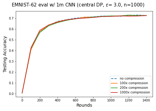
In Figure 4 and Figure 5, we present the accuracy results of the -CSGM algorithm (Algorithm 1) applied to F-EMNIST with varying cohort sizes, juxtaposed with the performance of the uncompressed Gaussian mechanism. Notably, our findings reveal that, on the whole, we can achieve compression exceeding 100x without a significant compromise in accuracy. Furthermore, as the cohort size increases, the impact of compression on utility diminishes. This implies that greater compression is feasible with larger values of . Similarly, in Figure 6, we delineate the accuracy outcomes for the Stack Overflow next-word prediction task across diverse values, maintaining a constant cohort size of .


Sparsified Gaussian Matrix Mechanism for DP-FTRL. In Figure 7 and Figure 8, we report the accuracy of SGMF (Algorithm 2) and the uncompressed matrix mechanism. We use the same factorization as in Denisov et al. (2022) with for epochs (due to the limited amount of clients), and we restart the mechanism and shuffle clients every epoch as in the approach in Kairouz et al. (2021b). We observe that for the matrix mechanism, the compression rates are generally less than DP-FedAvg, and the performance is more sensitive to server learning rates and clip norms.
Appendix D Proofs
D.1 Proof of Theorem 4.1
For any , it holds that
where (a) is due to the data processing inequality, and in (b) holds since and are independent across . Similarly, it holds that
For notational simplicity, let us define . Notice that implies .
Then for each , by Corollary 7 of Mironov et al. (2019),
where is a density function of and is a density function of .
For any integer , we have
where (a) is due to the generating function of normal distribution.
As a result, summing yields
First, observe that (1) is increasing and convex (since it is log-sum-exp), and (2) . Next, define as the unique sequence such that
-
•
for any ;
-
•
for any ;
-
•
.
Then, it is obvious that is a majorization555See https://en.wikipedia.org/wiki/Karamata%27s_inequality for a definition of “majorization”. of any such that and . Applying Karamata’s inequality666https://en.wikipedia.org/wiki/Karamata%27s_inequality yields
where the last inequality holds due to the convexity and the following Jensen’s inequality:
This establishes the theorem.
D.2 Proof of Lemma 5.2
To upper bound , observe that for any coordinate , depends solely on , and . Therefore,
Then, we claim that releasing is indeed an instance of (non-adaptive) subsampled Gaussian mechanism. By writing it in a vector form
| (6) |
it becomes clear as a subsampled Gaussian mechanism with sensitivity . Since and that is orthonormal, we have . Also, by the geometrical assumption of data matrix , it holds that and for all . Summing across and applying Theorem 4.1 yield
| (7) |
establishing the desired result.