Fractonic criticality in Rydberg atom arrays

Abstract

Fractonic matter can undergo unconventional phase transitions driven by the condensation of particles that move along subdimensional manifolds. We propose that this type of quantum critical point can be realized in a bilayer of crossed Rydberg chains. This system exhibits a transition between a disordered phase and a charge-density-wave phase with subextensive ground state degeneracy. The transition is described by a stack of critical Ising conformal field theories that become decoupled in the low-energy limit due to emergent subsystem symmetries. We discuss the unusual scaling properties and derive anisotropic correlators that provide signatures of subdimensional criticality in a realistic setup.

Introduction.— For decades, effective field theories have provided invaluable insight into quantum critical phenomena Hertz (1976); Sondhi et al. (1997); Sachdev (2011); Fradkin (2013). A general guiding principle is that the low-energy properties of a system close to a continuous phase transition are governed by nearly massless excitations. If these excitations propagate in all spatial directions, one expects universal scaling behavior once the correlation length diverges and microscopic details become irrelevant.

The standard continuum limit inherent in effective field theories has recently been challenged by the study of fracton phases of matter Nandkishore and Hermele (2019); Pretko et al. (2020); Gromov and Radzihovsky (2024). Fractonic systems are characterized by excitations that are completely immobile (fractons) or propagate along lower-dimensional subspaces (lineons and planons) Chamon (2005); Bravyi et al. (2011); Haah (2011); Vijay et al. (2016). In addition, fracton phases exhibit a subextensive ground state degeneracy. These properties are associated with subsystem symmetries, which can be either exact or emergent Lawler and Fradkin (2004); Nussinov and van den Brink (2015); You et al. (2020a); Gorantla et al. (2021) and play an important role in quantum phase transitions Mühlhauser et al. (2020); Poon and Liu (2021); Zhu et al. (2023); Lake and Hermele (2021); Rayhaun and Williamson (2023). In particular, continuous transitions can be driven by the condensation of lineons and planons, leading to the notion of subdimensional criticality Lake and Hermele (2021); Rayhaun and Williamson (2023). In this intriguing scenario, the transition is described by stacks of lower-dimensional critical theories, which decouple at low energies due to emergent subsystem symmetries.

In continuum descriptions of fractons Slagle and Kim (2017); Pretko (2018); Bulmash and Barkeshli (2018); Ma et al. (2018); Gromov (2019); You et al. (2020b); Seiberg and Shao (2020); Slagle (2021); Fontana et al. (2021); Sullivan et al. (2021), physical observables often depend on a short length scale related to a lattice regularization. The need for this regularization becomes apparent in theories with higher spatial derivatives and anisotropic scaling, an early example of which was the Bose metal in 2+1 dimensions Paramekanti et al. (2002); see also Ref. Seiberg and Shao (2021). In this case, the dispersion $\omega\sim k_{x}k_{y}$ of bosonic spin modes vanishes along lines in momentum space. As a consequence, high-momentum modes contribute to the low-energy physics, a phenomenon known as UV-IR mixing Seiberg and Shao (2020); Gorantla et al. (2021). Similar theories have been proposed for the fracton critical point in a higher-order topological transition You et al. (2022), the fractonic Berezinskii-Kosterlitz-Thouless transition in the plaquette-dimer model You and Moessner (2022); Grosvenor et al. (2023), and boundaries of fracton models Luo et al. (2022); Fontana and Pereira (2023). Crucially, UV-IR mixing imposes a modified renormalization group (RG) analysis Paramekanti et al. (2002); Lawler and Fradkin (2004); Xu and Moore (2005); Kapustin et al. (2018); You and Moessner (2022); Lake (2022); Grosvenor et al. (2023). In some contexts, the difficulties with scaling have been interpreted in terms of a dimensional reduction Lawler and Fradkin (2004); Xu and Moore (2005), whereby the two-dimensional (2D) model is viewed as an array of 1D systems. Despite the enormous interest sparked by fracton-like physics, a major obstacle to its observation is that the proposed lattice models typically contain multi-spin interactions that are hard to realize experimentally.

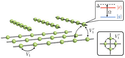
Figure 1: Setup with Rydberg atoms placed in chains that belong to two different planes. The atoms are toggled between the ground state $\left|g\right\rangle$ and a Rydberg state $\left|r\right\rangle$ by the external Rabi frequency $\Omega$ with a detuning $\Delta$. The leading interactions are the nearest-neighbor intrachain coupling $V_{1}$ and the interchain coupling $V_{1}^{\prime}$ around a crossing. The lower-right panel shows the top view of a single crossing.

In this work, we show that a fractonic transition can be observed in a realistic setup with Rydberg atom arrays, a versatile platform for the quantum simulation of long-sought phases of matter Browaeys and Lahaye (2020); Semeghini et al. (2021); Scholl et al. (2021); Surace et al. (2020); Verresen et al. (2021); Slagle et al. (2022); Myerson-Jain et al. (2022); Samajdar et al. (2023); Lee et al. (2023). Our setup consists of two layers of parallel chains with two-body interactions only; see Fig. 1. In the limit of decoupled chains, each chain displays a transition between a $\mathbb{Z}_{2}$-ordered charge density wave (CDW) and a disordered phase Fendley et al. (2004); Slagle et al. (2021). The 1D critical point is described by the Ising conformal field theory (CFT). We consider the regime in which the leading interchain interaction occurs at the crossings between perpendicular chains, and its strength can be controlled by varying the layer separation. We first show that the ordered phase of the 2D array retains a subextensive ground state degeneracy that can be understood in terms of an emergent subsystem symmetry. We refer to this phase as the fractonic CDW (fCDW). Analyzing the transition from the fCDW to the disordered phase, we find that the interlayer interaction is marginally irrelevant and the critical system displays 1D-like correlations.

The model.—We consider a model for $N$ trapped Rydberg neutral atoms, which in general are described by the Hamiltonian Saffman et al. (2010); Browaeys and Lahaye (2020)

$$H=\sum_{i=1}^{N}\left[\frac{\Omega}{2}(b_{i}+b^{\dagger}_{i})-\Delta n_{i}\right]+\sum_{1\leq i<j\leq N}V_{ij}n_{i}n_{j}\;,$$ (1)

where $b_{i},b^{\dagger}_{i}$ are annihilation and creation operators for hardcore bosons for the $i$-th atom, describing the ground state $|g\rangle_{i}$ and the Rydberg state $|r\rangle_{i}=b^{\dagger}_{i}|r\rangle_{i}$, with $n_{i}\equiv b^{\dagger}_{i}b^{\phantom{\dagger}}_{i}$. These states are coupled by external lasers with a Rabi frequency $\Omega$ and a detuning $\Delta>0$. The van der Waals interactions decay with the distance $R_{ij}$ between atoms as $V_{ij}=C_{6}R_{ij}^{-6}$.

The geometry of the lattice determines the leading interactions. In the setup of Fig. 1, the atoms are placed in 1D chains with lattice spacing $a$. Adjacent parallel chains are separated by a distance $d_{\parallel}=\nu a$, with an integer $\nu\geq 2$, and the layers are separated by $d_{\perp}$. The shortest distance between perpendicular chains occurs at a “crossing” (as viewed from above) where each atom is coupled symmetrically to a pair of atoms in the other layer. This model respects a $C_{4}$ lattice rotation symmetry, which also exchanges the layers, and a $\mathbb{Z}_{2}$ time-reversal symmetry defined as complex conjugation. Due to the fast decay of the interactions, we consider only two terms, $V_{1}$ and $V^{\prime}_{1}$, corresponding to nearest-neighbor intrachain and interchain couplings, respectively. The ratio $V^{\prime}_{1}/V_{1}=8[1+2(d_{\perp}/a)^{2}]^{-3}$ varies rapidly with the layer separation. Importantly, we neglect direct couplings between parallel chains. In Fig. 1, we represent the array with $\nu=2$ atoms between two crossings, but in practice it may be convenient to take $\nu>2$ to further suppress the interaction across the distance $d_{\parallel}$.

Phase diagram.—First, let us discuss the limit of decoupled chains obtained by taking $d_{\perp}\to\infty$. Introducing Pauli operators $Z_{i}=2n_{i}-1$ and $X_{i}=b_{i}^{\phantom{\dagger}}+b_{i}^{\dagger}$, we map the corresponding Hamiltonian $H_{0}$ to Ising chains with transverse and longitudinal fields Slagle et al. (2021):

$$H_{0}=\sum_{\ell=1}^{L_{x}+L_{y}}\sum_{m=1}^{L_{\ell}}(JZ_{m,\ell}Z_{m+1,\ell}+h_{X}X_{m,\ell}+h_{Z}Z_{m,\ell}),$$ (2)

where $J=V_{1}/4>0$, $h_{X}=\Omega/2$ and $h_{Z}=(V_{1}-\Delta)/2$. Here $\ell$ is a chain index, $m$ labels the position along the chain, and $L_{x}$ ($L_{y}$) is the number of vertical (horizontal) chains in the upper (lower) layer. We also define $L_{\ell}=\nu L_{y}$ for $1\leq\ell\leq L_{x}$ and $L_{\ell}=\nu L_{x}$ for $L_{x}+1\leq\ell\leq L_{x}+L_{y}$, and we assume periodic boundary conditions. The phase diagram of a single Ising chain has been studied numerically Ovchinnikov et al. (2003). For large $h_{X}$ or $h_{Z}$, the system is in a trivial disordered phase. For $h_{X},h_{Z}\ll J$, each chain locks into one of two CDW states represented by $|\cdots rgrg\cdots\rangle$ or $|\cdots grgr\cdots\rangle$, breaking translational invariance. Since each chain contributes with two states, there is a $2^{L_{x}+L_{y}}$-degenerate ground state manifold in this limit.

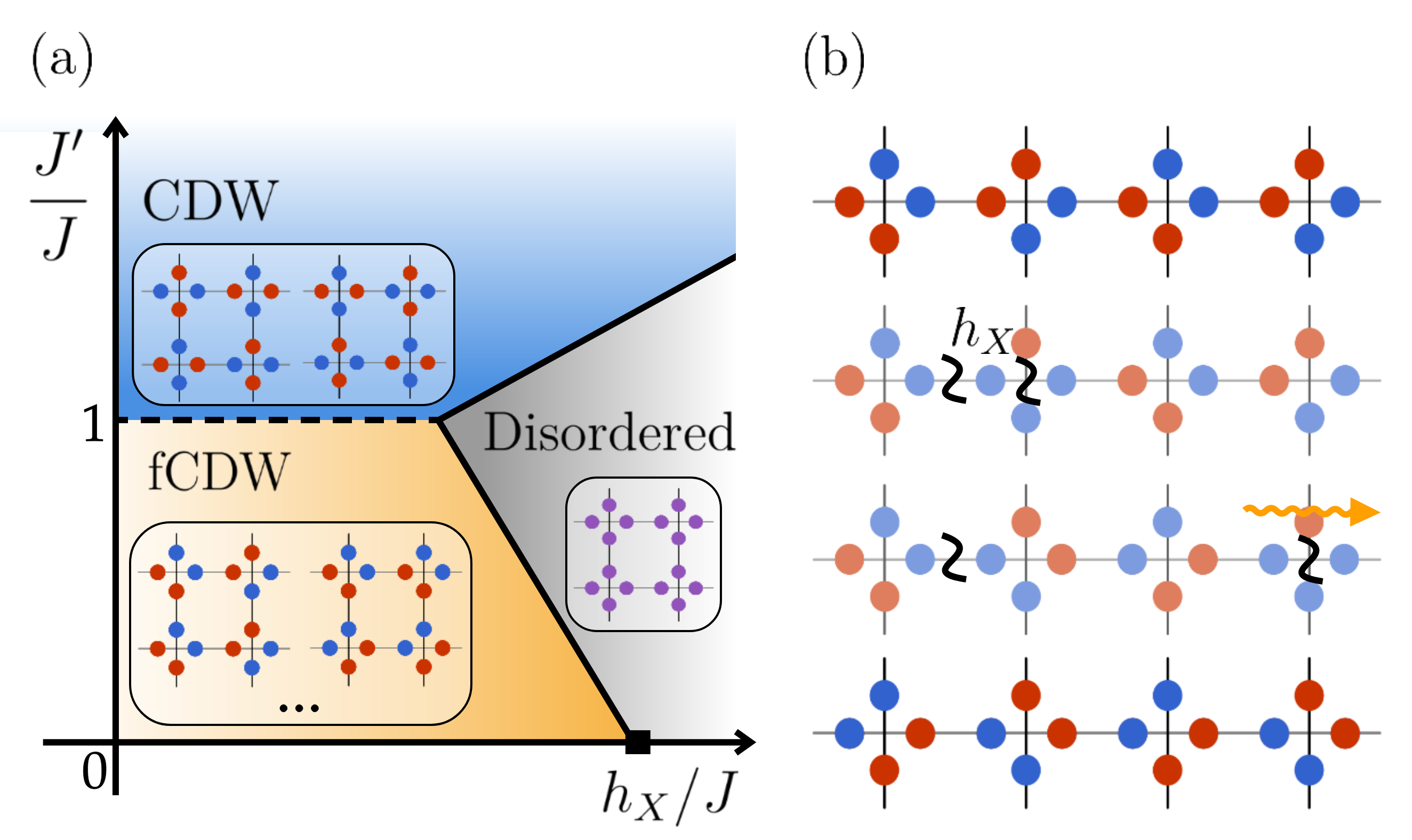
Figure 2: (a) Schematic phase diagram for a fixed value of $h_{Z}\ll J$. The local atomic states $\left|g\right\rangle$ and $\left|r\right\rangle$ in the ordered phases are represented by blue and red, respectively, while the disordered state is depicted in purple. The square on the $J^{\prime}=0$ axis marks the critical point of decoupled chains. Solid (dashed) lines denote second-order (first-order) transitions. (b) Given an fCDW ground state (top), reaching another ground state (bottom) requires creating and moving domain walls around the system.

To see the difference from a trivial stack of 1D states, we now turn on the interchain coupling $V^{\prime}_{1}>0$. In terms of spin variables, this term generates the perturbation

$$\delta H=J^{\prime}\sum_{\diamond}\sum_{\langle i,j\rangle\in\diamond}Z_{i}Z_{j}\;,$$ (3)

where $J^{\prime}=V^{\prime}_{1}/4$ and $\diamond$ stands for the bonds around a crossing. In addition, $V_{1}^{\prime}$ renormalizes the longitudinal field by $\delta h_{Z}=V^{\prime}_{1}/2$.

For $h_{X}=0$, the Hamiltonian $H=H_{0}+\delta H$ reduces to a classical Ising model. Increasing $J^{\prime}$, we encounter a level crossing between the $2^{Lx+L_{y}}$-degenerate ground states with energy $-2\nu JL_{x}L_{y}$ and twofold degenerate CDW states with energy $-[4J^{\prime}+2(\nu-2)J]L_{x}L_{y}$. In the latter, the four atomic states around each crossing alternate as $|rgrg\rangle$ or $|grgr\rangle$; see Fig. 2(a). In the classical model, this first-order transition happens at $J^{\prime}=J$. For $J^{\prime}\gg J$, one can go from the CDW to the disordered phase by increasing $h_{X}$; this transition belongs to the 3D Ising universality class, as found in other models of Rydberg arrays Samajdar et al. (2020); Yang and Xu (2022).

The exponential degeneracy of the ordered phase at $J^{\prime}<J$ is robust against quantum fluctuations induced by a weak transverse field. To see this, note that the low-lying gapped excitations in this regime are domain walls created in pairs by applying $\prod_{m_{1}\leq m\leq m_{2}}X_{m,\ell}$ on a given chain $\ell$. Two states in the ground state manifold can be coupled only by nonlocal processes that move domain walls around the system and correspond to “sliding” the spin chain configuration; see Fig. 2(b). Moreover, the domain walls in the subspace of low-lying excited states behave as lineons, as their motion is restricted to the chain direction, with dispersion $E_{\rm dw}(k)=2J-2h_{X}\cos(ka)+\mathcal{O}(h_{X}^{2})$.

Formally, the 1D nature of the excitation spectrum can be linked to an emergent subsystem symmetry. Consider the action of a translation in the $\ell$-th chain, $\mathcal{T}_{\ell}:\;Z_{m,\ell}\mapsto Z_{m+1,\ell}$, $X_{m,\ell}\mapsto X_{m+1,\ell}$. This is not an exact symmetry since it does not commute with the Hamiltonian in the presence of interchain couplings. However, an emergent symmetry can be defined by the condition Nussinov and van den Brink (2015)

$$[H,\mathcal{P}\mathcal{T}_{\ell}\mathcal{P}]=0,$$ (4)

where $\mathcal{P}$ is a projector onto a low-energy subspace. Both the ground-state and two-domain-wall subspaces are stabilized under the action of the group generated by $\mathcal{T}_{\ell}$. This means that the faithful symmetry action at low energies is given by $\mathbb{Z}_{2}^{L_{x}}\times\mathbb{Z}_{2}^{L_{y}}$, yielding the $2^{L_{x}+L_{y}}$ degenerate ground states. This exponential dependence on the linear size is characteristic of fracton models Nandkishore and Hermele (2019); Pretko et al. (2020), which motivates us to call this the fCDW phase.

Continuum limit.—We now move to construct an effective theory for the transition between the fCDW and the disordered phase. We begin by putting all the chains at criticality in the uncoupled regime, i.e., near the point represented by a square in Fig. 2. Each critical chain is described by an Ising CFT Slagle et al. (2021). This theory contains two classes of nontrivial primary operators: the energy operator $\varepsilon$ with conformal dimensions $\left(\frac{1}{2},\frac{1}{2}\right)$ and the spin field operator $\sigma$, with dimensions $\left(\frac{1}{16},\frac{1}{16}\right)$ Di Francesco et al. (1996). Lattice operators can be expanded as

$$X_{m,\ell}\sim\langle X_{m,\ell}\rangle\mathbb{I}+c_{\sigma}^{X}(-1)^{m}\sigma_{\ell}(x)+c_{\varepsilon}^{X}\varepsilon_{\ell}(x)+\cdots\;,$$ (5)

$$Z_{m,\ell}\sim\langle Z_{m,\ell}\rangle\mathbb{I}+c_{\sigma}^{Z}(-1)^{m}\sigma_{\ell}(x)+c_{\varepsilon}^{Z}\varepsilon_{\ell}(x)+\cdots\;,$$ (6)

where $\mathbb{I}$ is the identity, $x=ma$ is the position along the chain, $c_{\sigma}^{X,Z}$ and $c_{\varepsilon}^{X,Z}$ are nonuniversal real constants, and we omit higher-dimension operators. The $\mathbb{Z}_{2}$ symmetry of the Ising CFT corresponds to the 1D translation, under which the spin field $\sigma_{\ell}$ changes sign.

The low-energy Hamiltonian for decoupled chains can be written in terms of Majorana fermions. For a single chain, the holomorphic and anti-holomorphic parts of the stress tensor are given by $T=\frac{i}{2}\eta\partial_{x}\eta$ and $\bar{T}=-\frac{i}{2}\bar{\eta}\partial_{x}\bar{\eta}$, where $\eta(x)$ and $\bar{\eta}(x)$ are chiral Majorana fermions. We have $H_{\mathrm{1d}}=\int\mathrm{d}x\;[v(T+\bar{T})+m\varepsilon]$, where $v$ is the spin velocity and the energy operator $\varepsilon(x)=i\bar{\eta}\eta(x)$ appears in the mass term. Tuning to the critical point, we set $m=0$. Summing over all chains, we have

$$H_{0}\simeq\sum_{\lambda\in\{\text{h,v}\}}\sum_{\ell_{\lambda}=1}^{L_{\lambda}}\int\mathrm{d}x_{\lambda}\;v(T_{\lambda,\ell_{\lambda}}+\bar{T}_{\lambda,\ell_{\lambda}})(x_{\lambda}),$$ (7)

where we separate the contributions from horizontal (h) and vertical (v) chains by defining the labels $\ell_{\rm h}\in\{1,\cdots,L_{\rm h}\equiv L_{y}\}$, $\ell_{\rm v}\in\{1,\cdots,L_{\rm v}\equiv L_{x}\}$, and the coordinates $x_{\rm h}=x$ and $x_{\rm v}=y$.

Next, we add interchain couplings. Note that the interaction at a crossing has the form $J^{\prime}(Z_{m,\ell}+Z_{m+1,\ell})(Z_{m^{\prime},\ell^{\prime}}+Z_{m^{\prime}+1,\ell^{\prime}})$. In the continuum limit, this interaction selects the non-oscillating terms in Eq. (6). We obtain a term of the form $\sum_{k}\varepsilon_{\rm h}\varepsilon_{\rm v}(\mathbf{x}_{k})$, where $\mathbf{x}_{k}$ are the positions of the crossings. To deal with this interaction, we take a second continuum limit equivalent to sending $d_{\parallel}\to 0$; see the Supplemental Material (SM) SM . The effective Hamiltonian is given by

$$H\simeq\int\mathrm{d}^{2}\mathbf{x}\,v\left[\sum_{\lambda\in\{\rm h,\rm v\}}(T_{\lambda}+\bar{T}_{\lambda})(\mathbf{x})+\frac{g}{2\pi}\varepsilon_{\rm h}\varepsilon_{\rm v}(\mathbf{x})\right],$$ (8)

where $\mathrm{d}^{2}\mathbf{x}=\mathrm{d}x\mathrm{d}y$ and $g=\mathcal{O}(J^{\prime}/J)$. In the limit $g\to 0$, the fields in Eq. (8) act as coarse-grained versions of the operators in the Ising CFT. For instance, the energy operator has the correlator

$$\langle\varepsilon_{\rm h}(\mathbf{x}_{1})\varepsilon_{\rm h}(\mathbf{x}_{2})\rangle_{0}\simeq\frac{\delta(y_{1}-y_{2})}{|x_{1}-x_{2}|^{2}}.$$ (9)

At short distances, the delta function must be regularized as $\delta(0)\to\frac{1}{d_{\parallel}}$ to recover the 1D behavior. We note that the interchain coupling also generates a mass term $\int\mathrm{d}^{2}\mathbf{x}\,m(\varepsilon_{\rm h}+\varepsilon_{\rm v})$, but we can tune the mass to zero again by adjusting the longitudinal field.

The peculiar low-energy Hamiltonian in Eq. (8) inherits symmetries and dualities from the Ising chains. In the CFT, these symmetries are implemented by topological defect line operators Fröhlich et al. (2004); Chang et al. (2019). First, there is a Kramers-Wannier duality implemented by $D^{\sigma}=\bigotimes_{\ell}D_{\ell}^{\sigma}$, where $D_{\ell}^{\sigma}$ is the $\sigma$ defect of chain $\ell$ Fröhlich et al. (2004). The action of $D^{\sigma}$ takes $\varepsilon_{\ell}\mapsto-\varepsilon_{\ell}$, exchanging the correlators of the fCDW and the disordered phase, and becomes a global symmetry at the critical point. Second and more interestingly, an emergent $\mathbb{Z}_{2}^{L_{x}}\times\mathbb{Z}_{2}^{L_{y}}$ subsystem symmetry is manifested as the $\varepsilon$ defect, which acts on horizontal chains as $D^{\varepsilon}_{\ell_{\rm h}}\sigma_{\rm h}(x,\ell_{\rm h}a)=-\sigma_{\rm h}(x,\ell_{\rm h}a)D^{\varepsilon}_{\ell_{\rm h}}$, and similarly for vertical chains. This symmetry would be broken by the direct coupling between the order parameters of parallel chains. A lattice version of the algebra generated by $D^{\sigma}$ and $\{D^{\varepsilon}_{\ell}\}$ was recently discussed in Ref. Cao et al. (2023) as an example of a non-invertible subsystem symmetry, which strongly constrain the low-energy spectrum Seiberg et al. (2024). In fact, the existence of such line operators imposes that the Hilbert space of a perturbed 1+1 CFT cannot be trivially gapped Chang et al. (2019). This argument can be adapted to our subsystem realization when $L_{x}+L_{y}$ is odd; see the SM SM . Thus, we have the guarantee that Eq. (8) cannot have a trivial ground state even at strong coupling.

RG analysis.—We proceed to analyze the model perturbatively at $g\ll 1$, corresponding to $J^{\prime}\ll J$. The fate of the theory relies on the RG flow of the effective coupling $g(s)$ at length scale $s$ Cardy (1996). Power counting based on the correlator in Eq. (9) indicates that the coupling has effective scaling dimension $\Delta=3$ and is marginal at tree level. We calculate the beta function $\beta(g)$ to leading order using $a$ as a short-distance cutoff and introducing the large-distance cutoffs $D_{x}$ and $D_{y}$ for the $x$ and $y$ directions SM . We find that $g$ behaves as a marginally irrelevant coupling, with beta function

$$\frac{dg}{dl}=-\ln\left(\frac{D_{x}D_{y}}{a^{2}}\right)g^{3}+\cdots\;,$$ (10)

where $l=\ln(s/a)$ in the regime $a\ll s\ll\text{min}(D_{x},D_{y})$. Remarkably, the beta function depends explicitly on the ratio between the infrared and ultraviolet cutoffs, as found in models with UV-IR mixing Grosvenor et al. (2023); Kapustin et al. (2018). Physically, we expect $D_{x,y}\sim L_{x,y}a$, in which case the coefficient in Eq. (10) is proportional to $\ln(N_{c})$, where $N_{c}=L_{x}L_{y}\gg 1$ is the number of crossings. Here we adopt the perspective that experiments with Rydberg atoms must be performed on a finite system where $\ln(N_{c})$ is a constant of order 1, but there are notorious subtleties in taking the continuum and thermodynamic limits in the presence of UV-IR mixing; see Refs. Gorantla et al. (2021); Lake (2022).

Since the effective interchain coupling decreases at low energies, correlation functions can be calculated by perturbation theory. In particular, the leading contribution to correlators of crossed chains comes from the interaction at their crossing. We obtain SM

$$\langle\varepsilon_{\rm h}(x,0)\varepsilon_{\rm v}(0,y)\rangle\sim-\frac{g}{2(x^{2}|y|+|x|y^{2})}+\mathcal{O}(g^{3})\;.$$ (11)

Note the unusual spatially anisotropic power-law decay, a prominent feature of fractonic behavior You and Moessner (2022). This result captures the long-distance behavior of the correlation for the operator $Z_{j,\ell}+Z_{j+1,\ell}$, which can be measured by means of snapshots of the atomic states in Rydberg arrays Semeghini et al. (2021); Scholl et al. (2021).

Mean-field theory.— The perturbative RG analysis indicates that the fixed point of decoupled chains, $g=0$, is stable against the interchain coupling. To test this picture, we study a lattice model that reduces to Eq. (8) in the continuum limit but also regularizes the short-distance behavior. We consider the effective Hamiltonian

$$\tilde{H}=\sum_{\ell,m}(J_{\mathrm{e}}\tilde{Z}_{m,\ell}\tilde{Z}_{m+1,\ell}+h_{\mathrm{e}}\tilde{X}_{m,\ell})+J^{\prime}_{\mathrm{e}}\sum_{\diamond}\sum_{\langle i,j\rangle\in\diamond}\tilde{X}_{i}\tilde{X}_{j},$$ (12)

where $(J_{\mathrm{e}},h_{\mathrm{e}},J_{\mathrm{e}}^{\prime})$ can be choosen to match $v$ and $g$ in the continuum limit and we denote the new Pauli operators by $\tilde{X}_{i}$ and $\tilde{Z}_{i}$ to avoid confusion with the original lattice model. The advantage of Eq. (12) over the original model is that the subsystem symmetry is now manifest and on-site, and it can be implemented by $\prod_{j}\tilde{X}_{j,\ell}$ for each chain $\ell$. Moreover, we can perform a generalized Jordan-Wigner transformation Sachdev (2011); Crampé and Trombettoni (2013) and map the intrachain terms of Eq. (12) onto a stack of crossed Kitaev chains Kitaev (2001), in close connection with the Majorana representation in the field theory. We introduce two Majorana fermions at each site so that $\tilde{X}_{m,\ell}\mapsto i\gamma_{m,\ell}^{0}\gamma_{m,\ell}^{1}$. For the $\nu=2$ lattice, the unit cell contains 8 Majoranas denoted by $\gamma^{b}_{\mathbf{R},\alpha}$, where $b\in\{0,1\}$, $\mathbf{R}$ is the position of the unit cell, and $\alpha\in\{1,2,3,4\}$ labels the sites around the crossing; see the inset of Fig. 3. The symmetries act projectively due to the gauged fermion parity. Time reversal conjugates complex numbers and takes $\gamma^{b}_{j,\alpha}\mapsto(-1)^{b+1}\gamma^{b}_{j,\alpha}$, while the $C_{4}$ symmetry acts as $\gamma^{b}_{\mathbf{R},\alpha}\mapsto\gamma^{b^{\prime}}_{\mathbf{R}^{\prime},\alpha+1}$, where $b^{\prime}=b+\cos^{2}(\frac{\pi\alpha}{2})\text{ (mod 2)}$ and $\mathbf{R}^{\prime}$ is the rotated position.

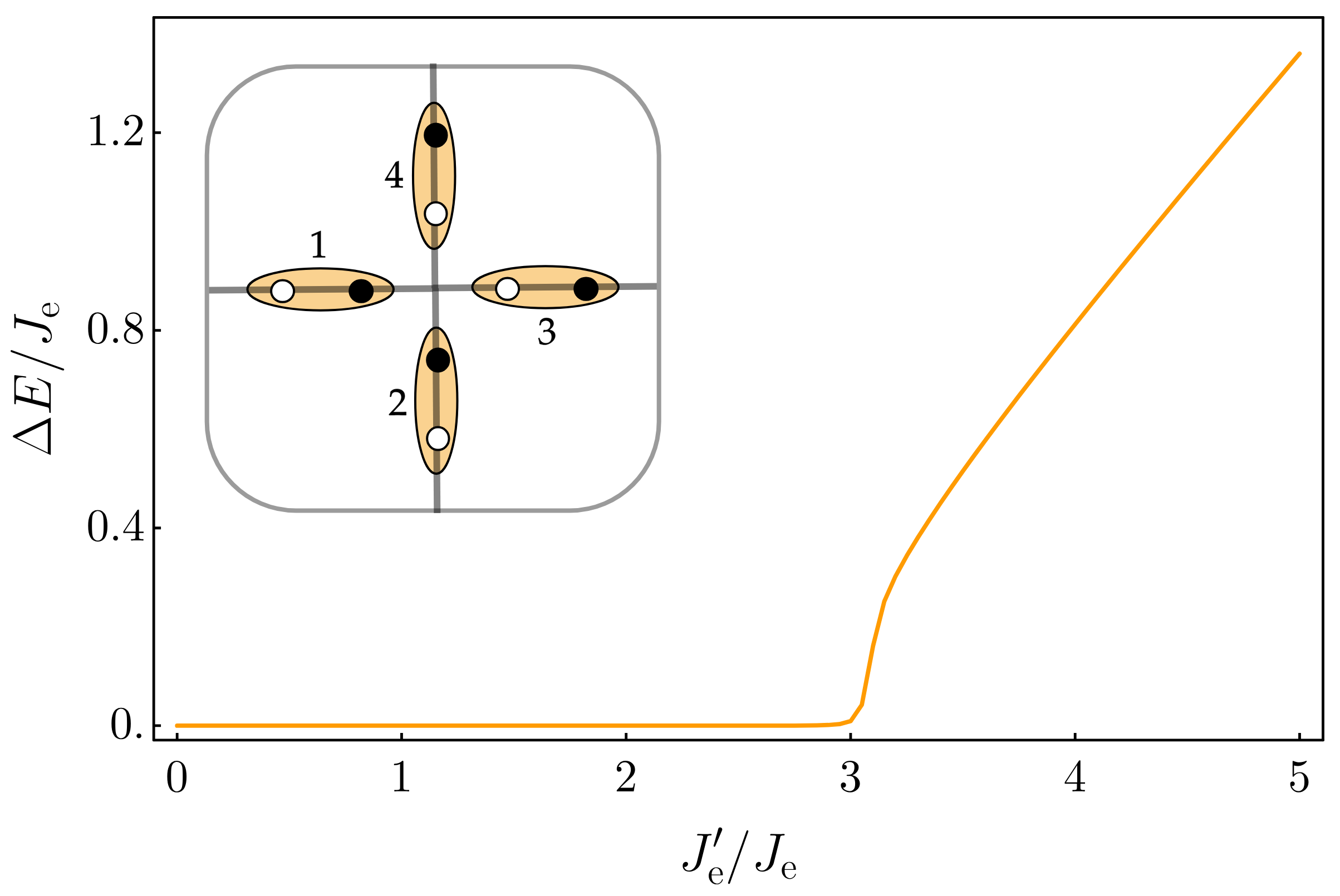
Figure 3: Majorana gap calculated by solving the mean-field equations for the model in Eq. (12). Inset: unit cell with eight Majorana modes $\gamma^{a}_{\mathbf{R},\alpha}$. Each site $\alpha\in\{1,2,3,4\}$ contains two modes, $b\in\{0,1\}$, represented by white and black dots, respectively.

The $J^{\prime}_{\rm e}$ interaction generates quartic terms in the fermionic representation. We treat this interacting model using a Majorana mean-field approach Rahmani and Franz (2019); Chen et al. (2019); Slagle et al. (2022). In this approach, a departure from the decoupled-chain fixed point is signalled by a spontaneous hybridization between modes in perpendicular chains. Imposing translation and time-reversal invariance, we have eight mean-field parameters allowed by symmetry:

$$A_{\alpha}=\langle i\gamma^{0}_{\mathbf{R},\alpha}\gamma^{1}_{\mathbf{R},\alpha+1}\rangle\;,\quad B_{\alpha}=\langle i\gamma^{1}_{\mathbf{R},\alpha}\gamma^{0}_{\mathbf{R},\alpha+1}\rangle\;.$$ (13)

We diagonalize the quadratic mean-field Hamiltonian and solve the self-consistency equations numerically SM . For $h_{\mathrm{e}}=J_{\mathrm{e}}$, we find that at for small $J_{\rm e}^{\prime}$ both $A_{\alpha}$ and $B_{\alpha}$ vanish and the fermionic spectrum is equivalent to critical Kitaev chains. As we increase $J_{e}^{\prime}$, the hybridization parameters eventually become nonzero and the 2D system develops an energy gap; see Fig. 3. In this regime, the $C_{4}$ symmetry is spontaneously broken. Note, however, that the gapped regime occurs at strong coupling, $J_{\rm e}^{\prime}>J_{e}$, where the connection with the original model via the effective field theory in Eq. (8) breaks down. While we cannot rule out additional phases around the tricritical point in Fig. 2, the mean-field theory confirms that the transition at weak to intermediate coupling is governed by the decoupled-chain fixed point. As characteristic of subdimensional criticality, at this fixed point we have emergent subsystem symmetries generated by both $D_{\ell}^{\varepsilon}$ and $D_{\ell}^{\sigma}$ for each chain in the continuum limit.

Conclusion.—We proposed a model for a fractonic quantum phase transition in Rydberg arrays. The critical point exhibits particles with restricted mobility, emergent subsystem symmetries, and anisotropic correlators that manifest the UV-IR mixing. Moving forward, it would be interesting to explore non-equilibrium dynamics near criticality, extensions to $\mathbb{Z}_{n}$-ordered phases Fendley et al. (2004), and to apply numerical methods Samajdar et al. (2021); Merali et al. (2024) to study the fCDW phase and the associated transitions. Our work represents a significant step towards the realization of fracton physics in quantum simulation platforms.

I Effective field theory for weakly coupled critical chains

In this section, we discuss the continuum limit for an array of Ising CFTs, the role of non-invertible subsystem symmetries, and the derivation of the perturbative renormalization group equation for the effective interchain coupling.

I.1 Continuum limit

First, we write down the Hamiltonian for the coupled chains described by $L_{x}+L_{y}$ copies of the Ising CFT:

$$H\simeq H_{0}+\delta H=\sum_{\lambda\in\{\mathrm{h,v}\}}\sum_{\ell_{\lambda}=1}^{L_{\lambda}}\int\mathrm{d}x_{\lambda}\,v\left(T_{\lambda,\ell_{\lambda}}+\bar{T}_{\lambda,\ell_{\lambda}}\right)\left(x_{\lambda}\right)+\frac{vg}{2\pi}\sum_{k=1}^{L_{x}L_{y}}\varepsilon_{\mathrm{h},\ell_{\mathrm{h}}^{k}}(x_{k})\varepsilon_{\mathrm{v},\ell_{\mathrm{v}}^{k}}(y_{k})\;,$$ (14)

where $\mathbf{x}_{k}=(x_{k},y_{k})$ labels the chain crossings, located on a square lattice with spacing $d_{\parallel}=\nu a$, and $\ell^{k}_{\mathrm{h,v}}$ labels the two chains participating in the crossing $\mathbf{x}_{k}$. This theory inherits a discrete translational symmetry when the continuum limit is taken only along the chain directions. The translations of all chains in the $x$ or $y$ directions are implemented by

$$\mathrm{T}_{x}: \quad O_{\text{v},\ell}(y)\mapsto O_{\text{v},\ell+1}(y),\quad O_{\text{h},\ell}(x)\mapsto O_{\text{h},\ell}(x+d_{\parallel}),$$ (15)

$$\mathrm{T}_{y}: \quad O_{\text{h},\ell}(x)\mapsto O_{\text{h},\ell+1}(x),\quad O_{\text{v},\ell}(y)\mapsto O_{\text{v},\ell}(y+d_{\parallel}).$$ (16)

The eigenstates of the effective Hamiltonian can be chosen as eigenstates of the translation operators $\mathrm{T}_{x}$ and $\mathrm{T}_{y}$. Thus, a state with energy $E$ also carries momentum $\mathbf{k}=(k_{x},k_{y})$ and satisfies

$$\mathrm{T}_{x}|E,\mathbf{k}\rangle =e^{ik_{x}d_{\parallel}}|E,\mathbf{k}\rangle\;,$$ (17)

$$\mathrm{T}_{y}|E,\mathbf{k}\rangle =e^{ik_{y}d_{\parallel}}|E,\mathbf{k}\rangle\;.$$ (18)

Hence, the corresponding Brillouin torus is defined by the quotients $k_{x}\sim k_{x}+2\pi/d_{\parallel}$ and $k_{y}\sim k_{y}+2\pi/d_{\parallel}$, meaning that the first Brillouin zone can be defined as $\mathbf{k}\in[-Q,Q]^{2}$, with $Q=\pi/d_{\parallel}$.

We now take a second continuum limit that describes observables when the relevant distances are larger than $d_{\parallel}$. This corresponds to the following assignments:

$$\sum_{\ell_{\mathrm{h}}=1}^{L_{y}}(\cdots)\mapsto\int\frac{\mathrm{d}y}{d_{\parallel}}\;(\cdots)\,;\quad\sum_{\ell_{\mathrm{v}}=1}^{L_{x}}(\cdots)\mapsto\int\frac{\mathrm{d}x}{d_{\parallel}}\;(\cdots)\,;\quad O_{\mathrm{h},\ell_{\mathrm{h}}}(x)\mapsto{d_{\parallel}}O_{\mathrm{h}}\left(x,d_{\parallel}\ell_{\mathrm{h}}\right)\,;\quad O_{\mathrm{v},\ell_{\mathrm{v}}}(y)\mapsto{d_{\parallel}}O_{\mathrm{v}}\left(d_{\parallel}\ell_{\mathrm{v}},y\right)\,,$$ (19)

where $O_{\lambda,\ell_{\lambda}}$ is a local operator in the Ising CFT in the copy of the $\ell_{\lambda}$-th chain. Following this prescription, we obtain

$$H\simeq\int\mathrm{d}^{2}\mathbf{x}\;v\left[\sum_{\lambda\in\{\mathrm{h},\mathrm{v}\}}(T_{\lambda}+\bar{T}_{\lambda})(\mathbf{x})+\frac{g}{2\pi}\varepsilon_{\mathrm{h}}\varepsilon_{\mathrm{v}}(\mathbf{x})\right]\;.$$ (20)

We also need a prescription for how to handle operator products in the limit $d_{\parallel}\to 0$. Consider correlators of decoupled Ising chains described by $H_{0}$. For example, the correlation function of the nontrivial primaries is given by

$$\langle\sigma_{\lambda,\ell_{\lambda}}(\mathbf{r}_{\lambda})\sigma_{\lambda,\ell_{\lambda}^{\prime}}(\mathbf{0})\rangle_{0}=\frac{\delta_{\ell_{\lambda},\ell_{\lambda}^{\prime}}}{|\mathbf{r}_{\lambda}|^{1/4}}\quad;\quad\langle\varepsilon_{\lambda,\ell_{\lambda}}(\mathbf{r}_{\lambda})\varepsilon_{\lambda,\ell_{\lambda}^{\prime}}(\mathbf{0})\rangle_{0}=\frac{\delta_{\ell_{\lambda},\ell_{\lambda}^{\prime}}}{|\mathbf{r}_{\lambda}|^{2}}\quad;\quad\lambda\in\{\text{h,v}\}\;,$$ (21)

where $\mathbf{r}_{\rm h}=(x,v\tau)$ and $\mathbf{r}_{\rm v}=(y,v\tau)$. All correlation functions between horizontal and vertical chains of the form $\langle O_{\rm h}O_{\rm v}\rangle_{0}$ vanish. In the 2D limit, the chain indices $\ell_{\rm h}$ and $\ell_{\rm v}$ must be replaced by continuous coordinates following the dictionary in Eq. (19). We adopt the following $C_{4}$-symmetric choice of the regulator:

$$\delta_{\ell_{\lambda},\ell_{\lambda}^{\prime}}\mapsto f_{\lambda}(x,y)\equiv\delta_{\lambda,\text{h}}\delta(y-d_{\parallel}\ell^{\prime}_{\rm h})+\delta_{\lambda,\text{v}}\delta(x-d_{\parallel}\ell^{\prime}_{\rm v})\;,$$ (22)

where we absorb nonuniversal prefactors into the normalization of the fields in the 2D limit. Now, the same correlation functions written in the ($2+1$)-dimensional theory become

$$\langle\sigma_{\lambda}(\mathbf{R})\sigma_{\lambda}(\mathbf{0})\rangle_{0}=\frac{f_{\lambda}(x,y)}{|\mathbf{R}|^{1/4}}\quad;\quad\langle\varepsilon_{\lambda}(\mathbf{R})\varepsilon_{\lambda}(\mathbf{0})\rangle_{0}=\frac{f_{\lambda}(x,y)}{|\mathbf{R}|^{2}}\quad;\quad\lambda\in\{\text{h,v}\}\;,$$ (23)

where $\mathbf{R}=(x,y,v\tau)$. Similarly, higher-point functions or correlators of other local operators (say, involving either descendants or the stress-energy tensor) can be regulated using Eq. (22).

I.2 Non-invertible subsystem symmetry and nontriviality of the ground state

We will argue that the non-invertible symmetry implies a nontrivial ground state for an odd number of chains. For this argument, it useful to view the field theory as a (macroscopic) collection of $L_{x}+L_{y}$ coupled Ising chains. As discussed in the main text, there is a $\mathbb{Z}_{2}^{L_{x}}\times\mathbb{Z}_{2}^{L_{y}}$ subsystem symmetry generated by the line operators $\{D^{\varepsilon}_{\ell}\}_{\ell=1}^{L_{x}+L_{y}}$ and a non-invertible symmetry generated by a Kramers-Wannier line $D^{\sigma}$ for $g\neq 0$. They form the following fusion algebra:

$$(D^{\varepsilon}_{\ell})\times(D^{\varepsilon}_{\ell})=1\quad;\quad\forall\ell\in\{1,\cdots,L_{x}+L_{y}\}\;,$$ (24)

$$(D^{\varepsilon}_{\ell})\times(D^{\sigma})=(D^{\sigma})\times(D^{\varepsilon}_{\ell})=D^{\sigma}\quad;\quad\forall\ell\in\{1,\cdots,L_{x}+L_{y}\}\;,$$ (25)

$$(D^{\sigma})\times(D^{\sigma})=\bigotimes_{\ell=1}^{L_{x}+L_{y}}(1+D^{\varepsilon}_{\ell})\;,$$ (26)

inherited from the Ising CFT fusion rules Fröhlich et al. (2004) (we omit the trivial fusion rules involving the identity line defect). Here, $\times$ denotes the fusion, and $\otimes$ takes the tensor product of symmetry lines on different chains. Note that the fusion rules depend on the number of chains, and therefore are not well defined in the thermodynamic limit. Similar behavior has been observed in the construction of the Kramers-Wannier defect (and the corresponding algebra with the $\mathbb{Z}_{2}$ symmetry) in the transverse-field Ising chain Seiberg et al. (2024) and in a lattice analog of Eqs. (24)-(26) Cao et al. (2023).

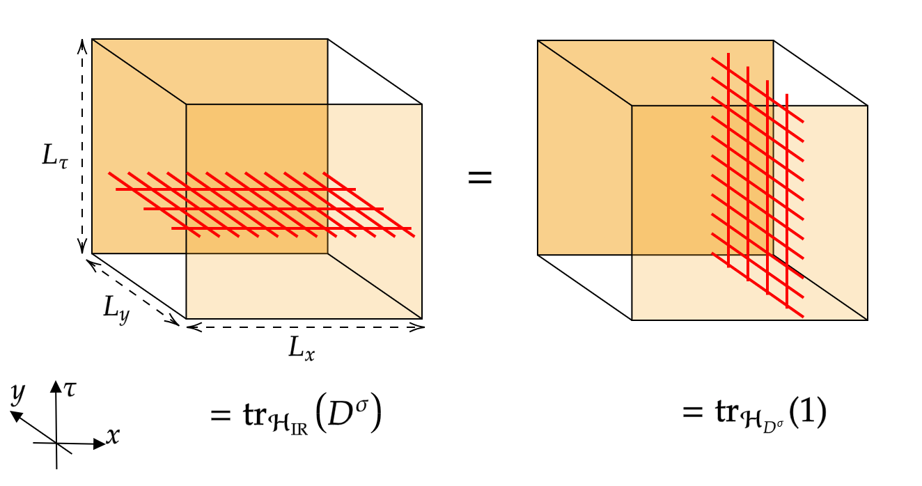
Figure 4: Two ways of inserting the Kramers-Wannier defect $D^{\sigma}$ in the path integral. On the left, the defect is defined on a constant-time slice, and its expectation value is computed in the infrared state. On the right, the defect is placed along the time direction, on a constant-$x$ slice. In this case, $L_{\tau}$ is taken such that $L_{\tau}=L_{x}$ to compute the dimension of the Hilbert space of the defect. At low energies, the results should match.

The expectation values of line operators are invariant under the RG flow. The reason is as follows. Given a vacuum $|\Omega\rangle$, we define the quantum dimensions $d^{\sigma}\equiv\langle D^{\sigma}\rangle=\langle\Omega|D^{\sigma}|\Omega\rangle$ and $d^{\varepsilon}_{S}\equiv\langle\otimes_{\ell\in S}D^{\varepsilon}_{\ell}\rangle=\langle\Omega|\otimes_{\ell\in S}D^{\varepsilon}_{\ell}|\Omega\rangle$ for any subset $S\subseteq\{1,\cdots,L_{x}+L_{y}\}$. It follows that the fusion ring generated by the relations above, $\{d^{\sigma},\{d^{\varepsilon}_{S}\}_{S\subseteq\{1,\cdots,L_{x}+L_{y}\}}\}$ satisfies polynomial equations with integer coefficients. Therefore, they must be RG invariants. This is completely analogous to the argument made in Ref. Chang et al. (2019) in the context of $(1+1)$-dimensional QFTs.

First, for $g=0$, consider the $(\mathrm{Ising})^{\otimes(L_{x}+L_{y})}$ theory. By radial quantization, the ground state of this theory is $|\Omega_{0}\rangle\equiv\otimes_{\ell=1}^{L_{x}+L_{y}}|1\rangle_{\ell}$, where $|1\rangle_{\ell}$ is the state corresponding to the identity operator of the $\ell$-th chain. It is also known that the Kramers-Wannier defect has a quantum dimension of $\sqrt{2}$ since $D^{\sigma}_{\ell}|1\rangle_{\ell}=\sqrt{2}|1\rangle_{\ell}$. Therefore,

$$D^{\sigma}|\Omega_{0}\rangle\equiv\langle D^{\sigma}\rangle_{0}|\Omega_{0}\rangle=2^{(L_{x}+L_{y})/2}|\Omega_{0}\rangle\;.$$ (27)

Thus, even for $g\neq 0$, we have $d^{\sigma}=\langle D^{\sigma}\rangle=\langle D^{\sigma}\rangle_{0}=2^{(L_{x}+L_{y})/2}$ by the arguments above.

Suppose now that there is a unique ground state in the infrared described by a Hilbert space $\mathcal{H}_{\mathrm{IR}}$ such that $\mathrm{dim}(\mathcal{H}_{\mathrm{IR}})=1$. In this case,

$$d^{\sigma}=\langle D^{\sigma}\rangle=\mathrm{tr}_{\mathcal{H}_{\mathrm{IR}}}(D^{\sigma}).$$ (28)

Physically, it is useful to understand this equation in the path integral approach, where the trace corresponds to taking periodic boundary conditions in the time direction. Thus, $d^{\sigma}$ computes the expectation value of $D^{\sigma}$ on a time slice. The same amplitude can be computed by inserting the mesh in the time direction. In the path integral picture, this works by slicing the Euclidean time direction into either $T=\Delta_{x}\tau L_{x}$ or $T=\Delta_{y}\tau L_{y}$, depending on whether the mesh is positioned in the $x$ or $y$ direction, making the action of $D^{\sigma}$ well defined; see Fig. 4.

As a consequence, one can interpret the quantization of $d^{\sigma}$ as counting the dimension of a twisted Hilbert space $\mathcal{H}_{D^{\sigma}}$, where the operators (and corresponding states) have twisted boundary conditions with the action of $D^{\sigma}$. But this is the same as computing the corresponding quantum dimension:

$$d^{\sigma}=\langle D^{\sigma}\rangle=\mathrm{tr}_{\mathcal{H}_{D^{\sigma}}}(1)\;,$$ (29)

leading to a contradiction for $L_{x}+L_{y}$ odd, since the rhs is a non-negative integer and the lhs is not. Therefore, the infrared Hilbert space must have more than one state.

I.3 Renormalization group

We now derive the perturbative RG equations and the corresponding corrections to observables. Consider the partition function associated with the Hamiltonian in Eq. (20). The path integral can be written in terms of the free partition function $Z_{0}$, defined at $g=0$, as:

$$\frac{Z}{Z_{0}}=\left\langle e^{-\frac{g}{2\pi}\int d^{3}\mathbf{R}\;\varepsilon_{\mathrm{h}}\varepsilon_{\mathrm{v}}(\mathbf{R})}\right\rangle_{0}=1-gI^{(1)}+\frac{g^{2}}{2!}I^{(2)}-\frac{g^{3}}{3!}I^{(3)}+\cdots\;,$$ (30)

where $d^{3}\mathbf{R}=dxdyd(v\tau)$ is the volume element in Euclidean spacetime, $\langle\cdots\rangle_{0}$ denotes the expectation value in the free theory, and in the last equality we expressed the ratio in a perturbative expansion. The corresponding integrals up to the third order are given by

$$I^{(1)} =\frac{1}{2\pi}\int d^{3}\mathbf{R}\;\langle\varepsilon_{\mathrm{h}}\varepsilon_{\mathrm{v}}(\mathbf{R})\rangle_{0}\;,$$ (31)

$$I^{(2)} =\frac{1}{(2\pi)^{2}}\int d^{3}\mathbf{R}_{1}d^{3}\mathbf{R}_{2}\;\langle\varepsilon_{\mathrm{h}}\varepsilon_{\mathrm{v}}(\mathbf{R}_{1})\varepsilon_{\mathrm{h}}\varepsilon_{\mathrm{v}}(\mathbf{R}_{2})\rangle_{0}\;,$$ (32)

$$I^{(3)} =\frac{1}{(2\pi)^{3}}\int d^{3}\mathbf{R}_{1}d^{3}\mathbf{R}_{2}d^{3}\mathbf{R}_{3}\;\langle\varepsilon_{\mathrm{h}}\varepsilon_{\mathrm{v}}(\mathbf{R}_{1})\varepsilon_{\mathrm{h}}\varepsilon_{\mathrm{v}}(\mathbf{R}_{2})\varepsilon_{\mathrm{h}}\varepsilon_{\mathrm{v}}(\mathbf{R}_{3})\rangle_{0}.$$ (33)

The integrals must be regularized by imposing a UV cutoff. We will choose a specific cutoff scheme following the approach explained in Ref. Cardy (1996). The three steps behind the perturbative renormalization group are: (1) perform an infinitesimal RG transformation, where the short-distance cutoff $a$ is renormalized as $a\to a(1+dl)$, (2) discard all contributions which are $\mathcal{O}(dl^{2})$ or higher; (3) impose that the partition function must remain invariant, reading off the corresponding renormalization conditions. This is the standard approach in the study of scale-invariant fixed points, but we will encounter difficulties related to UV-IR mixing when we perturb around the fixed point of decoupled crossed chains.

The first-order term is invariant under the scaling, implying that the perturbation is tree-level marginal as mentioned in the main text. The second-order term only contributes to the renormalization of irrelevant interactions, such as $\varepsilon_{\mathrm{h}}\partial_{x}\varepsilon_{\mathrm{h}}$ and $\varepsilon_{\mathrm{v}}\partial_{x}\varepsilon_{\mathrm{v}}$. The renormalization of the coupling appears at third order or two-loop level. By Wick’s theorem, the contribution in Eq. (33) can be written as

$$I^{(3)}=\frac{3}{(2\pi)^{3}}\int d^{3}\mathbf{R}_{1}d^{3}\mathbf{R}_{2}d^{3}\mathbf{R}_{3}\;\left[\langle\varepsilon_{\mathrm{h}}(\mathbf{R}_{1})\varepsilon_{\mathrm{v}}(\mathbf{R}_{3})\rangle_{0}\langle\varepsilon_{\mathrm{v}}(\mathbf{R}_{1})\varepsilon_{\mathrm{v}}(\mathbf{R}_{2})\rangle_{0}\langle\varepsilon_{\mathrm{h}}(\mathbf{R}_{2})\varepsilon_{\mathrm{h}}(\mathbf{R}_{3})\rangle_{0}+(\mathrm{h}\leftrightarrow\mathrm{v})\right],$$ (34)

where the combinatorial factor comes from exchanging the positions of the interaction vertices. Taking the leading contributions as $\mathbf{R}_{3}\to\mathbf{R}_{1}$ and using the correlator for decoupled chains, we obtain

$$I^{(3)} = \frac{6}{(2\pi)^{3}}\int d^{3}\mathbf{R}\,\langle\varepsilon_{\mathrm{h}}\varepsilon_{\mathrm{v}}(\mathbf{R})\rangle_{0}\int d^{3}\mathbf{R}_{12}d^{3}\mathbf{R}_{13}\;\frac{\delta(x_{12})}{|\mathbf{R}_{12}|^{2}}\frac{\delta(y_{23})}{|\mathbf{R}_{23}|^{2}}$$ (35)

$$= \frac{6}{(2\pi)^{3}}\int d^{3}\mathbf{R}\,\langle\varepsilon_{\mathrm{h}}\varepsilon_{\mathrm{v}}(\mathbf{R})\rangle_{0}\int dy_{12}d(v\tau_{12})dx_{23}d(v\tau_{23})\;\frac{1}{y_{12}^{2}+(v\tau_{12})^{2}}\frac{1}{x_{23}^{2}+(v\tau_{23})^{2}}.$$

This is the point where the calculation departs from the standard scheme for conformally invariant fixed points. Note the anisotropic dependence of the integrand in the four-dimensional space spanned by $(x_{12},y_{23},\tau_{12},\tau_{23})$. Since the integrand is singular for $y_{12}=\tau_{12}=0$ or $x_{23}=\tau_{23}=0$, we cannot simply integrate out a spherical shell in the four-dimensional space. This dependence can be traced back to the 1D nature of the correlators at the decoupled-chain fixed point. We proceed by integrating out arbitrary time differences, $-\infty<\tau_{12},\tau_{23}<\infty$, while keeping a short-distance cutoff. We obtain

$$I^{(3)} = \frac{3}{4\pi}\int d^{3}\mathbf{R}_{1}\,\langle\varepsilon_{\mathrm{h}}\varepsilon_{\mathrm{v}}(\mathbf{R})\rangle_{0}\int_{a}^{D_{y}}\frac{dy_{12}}{|y_{12}|}\int_{a}^{D_{x}}\frac{dx_{23}}{|x_{23}|}=\frac{3}{\pi}\ln\left(\frac{D_{x}}{a}\right)\ln\left(\frac{D_{y}}{a}\right)I^{(1)}\;,$$ (36)

where we imposed both the spatial UV cutoff $a$ and IR cutoffs $D_{x}$ and $D_{y}$. Note the peculiar double logarithmic dependence, which diverges for $D_{x}\to\infty$ or $D_{y}\to\infty$. The scales $D_{x}$ and $D_{y}$ can be interpreted as being of the order of the linear system size in the $x$ and $y$ directions, respectively. As discussed in the context of UV-IR mixing in Bose-metal-like models Gorantla et al. (2021); Lake (2022), the result may depend on how we handle the thermodynamic limit along with the continuum limit.

We can now perform the renormalization steps on the term in Eq. (36). Rescaling $a\to a(1+dl)$, we obtain $I^{(3)}\to I^{(3)}+\delta I^{(3)}+\mathcal{O}(dl^{2})$, where

$$\delta I^{(3)}=-6\ln\left(\frac{D_{x}D_{y}}{a^{2}}\right)dl\;I^{(1)}\;.$$ (37)

The corresponding change in the pertubative expansion defined in Eq. (30) can be written as

$$\frac{Z}{Z_{0}}\to 1-\frac{1}{2\pi}\left[g-\ln\left(\frac{D_{x}D_{y}}{a^{2}}\right)g^{3}dl\right]I^{(1)}+\frac{g^{2}}{2!}I^{(2)}-\frac{g^{3}}{3!}I^{(3)}+\cdots\;,$$ (38)

where we neglected irrelevant terms stemming from $I^{(2)}$. Imposing invariance under the RG transformation, we see that the coupling is renormalized as $g\to g+dg$, with the RG equation:

$$\frac{dg}{dl}=-\ln\left(\frac{D_{x}D_{y}}{a^{2}}\right)g^{3}+\cdots\;.$$ (39)

If we take $D_{x}\sim L_{x}a$ and $D_{y}\sim L_{y}a$, prefactor in the beta function is proportional to $\ln(N_{c})$, where $N_{c}=L_{x}L_{y}$ is the number of chain crossings.

Assuming that the running coupling is small but finite, we can compute corrections to observables at long distances. Consider the correlator for the energy operator in a pair of horizontal and vertical chains, which to lowest order in $g$ is given by

$$\left\langle\varepsilon_{\mathrm{h}}(x,0)\varepsilon_{\mathrm{v}}(0,y)\right\rangle\simeq-\frac{g}{2\pi}\int d^{3}\mathbf{R}\;\langle\varepsilon_{\mathrm{h}}(x,0)\varepsilon_{\mathrm{v}}(0,y)\varepsilon_{\mathrm{h}}\varepsilon_{\mathrm{v}}(\mathbf{R})\rangle_{0}+\cdots\;,$$ (40)

where we ignored all higher-order terms. Taking the coordinates as $\mathbf{R}=(R_{x},R_{y},v\tau)$, the integrand can be directly evaluated as

$$\langle\varepsilon_{\mathrm{h}}(x,0)\varepsilon_{\mathrm{v}}(0,y)\varepsilon_{\mathrm{h}}\varepsilon_{\mathrm{v}}(\mathbf{R})\rangle_{0}=\langle\varepsilon_{\mathrm{h}}(x,0)\varepsilon_{\mathrm{h}}(\mathbf{R})\rangle_{0}\langle\varepsilon_{\mathrm{v}}(0,y)\varepsilon_{\mathrm{v}}(\mathbf{R})\rangle_{0}=\frac{\delta(R_{y})\delta(R_{x})}{[(x-R_{x})^{2}+R_{y}^{2}+v^{2}\tau^{2}][R_{x}^{2}+(y-R_{y})^{2}+v^{2}\tau^{2}]}\;.$$ (41)

Integrating over the spatial and temporal coordinates, we get our first-order result:

$$\langle\varepsilon_{\mathrm{h}}(x,0)\varepsilon_{\mathrm{v}}(0,y)\rangle\simeq-\frac{g}{2(|x|y^{2}+|y|x^{2})}+\mathcal{O}(g^{2})\;.$$ (42)

This form of the correlator can be explained by symmetry and scaling arguments. Since the energy operator in the (2+1)-dimensional theory behaves as having the effective scaling dimension $\Delta_{\varepsilon}=3/2$, see Eq. (9) of the main text, we expect $\langle\varepsilon_{\mathrm{h}}(x,0)\varepsilon_{\mathrm{v}}(0,y)\rangle\sim[f(x,y)]^{-1}$, where $f(x,y)$ is a homogeneous function of degree 3 in the spatial coordinates. The $C_{4}$ and reflection symmetries imply $f=f(|x|,|y|)=f(|y|,|x|)$. So far, these conditions fix the form $f=c_{1}(|x|^{3}+|y|^{3})+c_{2}(|x|y^{2}+|y|x^{2})$, where $c_{1}$ and $c_{2}$ are dimensionless constants. In addition, the correlator must be singular for $x\to 0$ or $y\to 0$, which corresponds to taking two points on the same chain. When one of the coordinates is of the order or the lattice spacing, say $x\sim a$, we must recover the correlation function of the Ising CFT, $f(a,y)\sim y^{2}$ for $|y|\gg a$. This last constraint imposes $c_{1}=0$, and we are left with $f\sim|x|y^{2}+|y|x^{2}$.

Let us analyze how the running coupling changes the behavior of the correlation function. If we integrate Eq. (39) treating $C\equiv\ln(D_{x}D_{y}/a^{2})>0$ as a constant coefficient, we obtain for the effective coupling at length scale $s$:

$$g^{2}(s)=\frac{g_{0}^{2}}{1+2Cg^{2}_{0}\ln(s/a)}\simeq\frac{1}{2C}[\ln(s/a))]^{-1}\;.$$ (43)

Here we have approximated the result in the regime $ae^{1/(2Cg_{0}^{2})}\ll s\ll D_{x},D_{y}$, where the effective coupling becomes independent of the bare coupling constant $g_{0}$. Substituting this approximation back in the correlation function and setting $s=[f(x,y)]^{1/3}$ for the characteristic length scale, we obtain

$$\langle\varepsilon_{\mathrm{h}}(x,0)\varepsilon_{\mathrm{v}}(0,y)\rangle\sim-\sqrt{\frac{3}{8C}}\frac{\left[\ln\left(\frac{x^{2}|y|+|x|y^{2}}{a^{3}}\right)\right]^{-\frac{1}{2}}}{x^{2}|y|+|x|y^{2}}+\mathcal{O}(g^{2})\;.$$ (44)

Therefore, the crossed-chain correlator acquires a logarithmic correction at large distances.

II Mean-field theory

In this section, we describe the mean-field approach for the effective lattice model. As defined in the main text, we consider

$$\tilde{H}=\sum_{\ell,m}(J_{\mathrm{e}}\tilde{Z}_{m,\ell}\tilde{Z}_{m+1,\ell}+h_{\mathrm{e}}\tilde{X}_{m,\ell})+J^{\prime}_{\mathrm{e}}\sum_{\diamond}\sum_{\langle i,j\rangle\in\diamond}\tilde{X}_{i}\tilde{X}_{j}\;.$$ (45)

The explicit $\mathbb{Z}_{2}^{L_{x}}\times\mathbb{Z}_{2}^{L_{y}}$ symmetry, generated by the chain parities $\prod_{m}\tilde{X}_{m,\ell}$, takes $\tilde{Z}_{m,\ell}\mapsto-\tilde{Z}_{m,\ell}$ for all sites $m$ that belong to a given chain $\ell$. We employ a generalization of the Jordan-Wigner transformation given by

$$\tilde{X}_{m,\ell}=i\gamma^{0}_{m,\ell}\gamma^{1}_{m,\ell}\;,\qquad\tilde{Y}_{m,\ell}=\eta_{\ell}B_{m,\ell}\gamma^{0}_{m,\ell}\qquad\tilde{Z}_{m,\ell}=\eta_{\ell}B_{m,\ell}\gamma^{1}_{mi,\ell}\;.$$ (46)

Here $\gamma^{b}_{m,\ell}$, with $b\in\{0,1\}$, are Majorana fermions satisfying $\{\gamma^{b}_{m,\ell},\gamma^{b^{\prime}}_{m^{\prime},\ell^{\prime}}\}=2\delta^{bb^{\prime}}\delta_{m,m^{\prime}}\delta_{\ell,\ell^{\prime}}$. To ensure the Pauli algebra of physical operators, we have introduced the string operators

$$\quad B_{m,\ell}=\prod_{m^{\prime}\leq m}i\gamma^{0}_{m^{\prime},\ell}\gamma^{1}_{m^{\prime},\ell}\;,$$ (47)

and the chain-dependent Klein factors $\eta_{\ell}$ Crampé and Trombettoni (2013) that obey $\{\eta_{\ell},\eta_{\ell^{\prime}}\}=2\delta_{\ell,\ell^{\prime}}$ and commute with the “dynamical” Majorana modes $\gamma^{b}_{m,\ell}$. The Hamiltonian is written in terms of Majorana fermions as

$$\tilde{H}=\sum_{\ell,m}(iJ_{\mathrm{e}}\gamma^{1}_{m,\ell}\gamma^{0}_{m+1,\ell}+ih_{\mathrm{e}}\gamma^{0}_{m,\ell}\gamma^{1}_{m,\ell})-J^{\prime}_{\mathrm{e}}\sum_{\diamond}\sum_{\langle i,j\rangle\in\diamond}\gamma^{0}_{i}\gamma^{1}_{i}\gamma^{0}_{j}\gamma^{1}_{j}\;.$$ (48)

For $J^{\prime}_{\mathrm{e}}=0$, we identify a stack of Kitaev chains that result from the fermionization of the Ising chains.

Hereafter, we adopt the labelling of the Majorana modes $\gamma^{b}_{\mathbf{R},\alpha}$ according to the unit cell introduced in the main text. Time reversal and lattice rotation symmetries act projectively on Majorana fermions as defined in the main text. Since the interactions couple different sites at the same crossing, the natural mean-field parameters are $\langle i\gamma^{b}_{\mathbf{R},\alpha}\gamma^{b^{\prime}}_{\mathbf{R},\alpha+1}\rangle$. Note that the mean-field decoupling of the interaction also generates the on-site amplitudes $\langle i\gamma^{0}_{\mathbf{R},\alpha}\gamma^{1}_{\mathbf{R},\alpha}\rangle$, but their effect can be absorbed into a renormalization of the transverse field $h_{\rm e}$, which must be tuned to the critical point. We assume that the mean-field ansatz at criticality respects time reversal invariance because this symmetry is preserved both in the fCDW and in the disordered phase. Time reversal invariance implies the vanishing of amplitudes diagonal in the upper index, $\langle i\gamma^{0}\gamma^{0}\rangle=\langle i\gamma^{1}\gamma^{1}\rangle=0$. Imposing translational symmetry and considering the possibility of breaking the rotation symmetry (since the fCDW breaks $C_{4}$), we are left with eight amplitudes, defined as

$$A_{\alpha}\equiv\langle i\gamma^{0}_{\mathbf{R},\alpha}\gamma^{1}_{\mathbf{R},\alpha+1}\rangle\quad;\quad B_{\alpha}\equiv\langle i\gamma^{1}_{\mathbf{R},\alpha}\gamma^{0}_{\mathbf{R},\alpha+1}\rangle\;.$$ (49)

The interaction can then be decoupled as

$$J^{\prime}_{\mathrm{e}}\sum_{\mathbf{R}}\sum_{\alpha_{o}\in\{1,3\}}i\gamma^{0}_{\mathbf{R},\alpha_{e}}\gamma^{1}_{\mathbf{R},\alpha_{o}}\sum_{\alpha_{e}\in\{2,4\}}i\gamma^{0}_{\mathbf{R},\alpha_{e}}\gamma^{1}_{\mathbf{R},\alpha_{e}}\to J^{\prime}_{\mathrm{e}}\sum_{\mathbf{R},\alpha}(A_{\alpha}i\gamma^{1}_{\mathbf{R},\alpha}\gamma^{0}_{\mathbf{R},\alpha+1}+B_{\alpha}i\gamma^{0}_{\mathbf{R},\alpha}\gamma^{1}_{\mathbf{R},\alpha+1})\;.$$ (50)

This decoupling leads to the mean-field Hamiltonian $\tilde{H}_{\mathrm{MF}}$, which is quadratic in fermions. We introduce momentum modes as

$$\gamma^{a}_{\mathbf{R},\alpha}=\sqrt{\frac{2}{N_{c}}}\sum_{\mathbf{k}\in\text{BZ}}e^{i\mathbf{k}\cdot\mathbf{R}}\gamma^{a}_{\mathbf{k},\alpha}\;,$$ (51)

where $\mathrm{BZ}\equiv[-\pi/d_{\parallel},\pi/d_{\parallel}]^{2}$, with $d_{\parallel}=2a$, stands for the Brillouin zone of the square lattice with $N_{c}=L_{x}L_{y}$ unit cells. For Majorana fermions, we have the relation $\gamma^{a}_{-\mathbf{k},\alpha}=(\gamma^{a}_{\mathbf{k},\alpha})^{\dagger}$, which allows us to restrict to modes in one half of the Brillouin zone, say $\mathrm{HBZ}\equiv[-\pi/d_{\parallel},\pi/d_{\parallel}]\times[0,\pi/d_{\parallel}]$. These complex fermion operators satisfy $\{\gamma^{b}_{\mathbf{k},\alpha},\gamma^{b^{\prime}}_{\mathbf{k}^{\prime},\alpha^{\prime}}\}=\delta^{bb^{\prime}}\delta_{\mathbf{k},\mathbf{k}^{\prime}}\delta_{\alpha,\alpha^{\prime}}$.

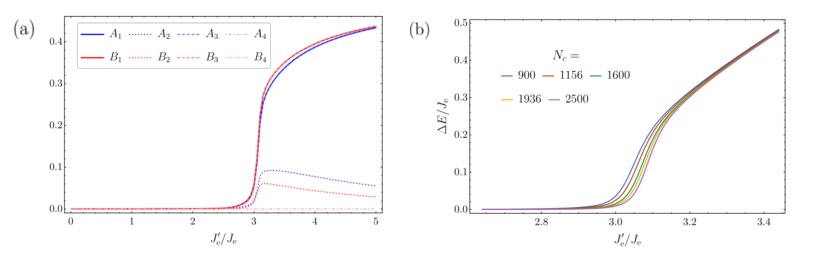
Figure 5: Results from the mean-field theory. (a) Solutions of the eight mean-field parameters in Eqs. (55) and (56), computed for $N_{c}=50\times 50=2500$ unit cells. Note that the $C_{4}$-related parameters acquire different values for $J^{\prime}_{\mathrm{e}}/J_{\mathrm{e}}\gtrsim 3$. (b) Fermion gap calculated from the mean-field solution for different system sizes.

The mean-field Hamiltonian can be cast in the form

$$\tilde{H}_{\mathrm{MF}}=\sum_{\mathbf{k}\in\mathrm{HBZ}}\Psi^{\dagger}_{\mathbf{k}}\mathcal{H}_{\mathrm{MF}}(\mathbf{k})\Psi^{\phantom{\dagger}}_{\mathbf{k}}\;,$$ (52)

where $\Psi_{\mathbf{k}}=(\gamma^{0}_{\mathbf{k},1},\;\gamma^{0}_{\mathbf{k},2},\;\cdots,\gamma^{1}_{\mathbf{k},3},\;\gamma^{1}_{\mathbf{k},4})^{T}$ is an eight-component spinor and $\mathcal{H}_{\mathrm{MF}}(\mathbf{k})$ is an $8\times 8$ Hermitean matrix that depends on $J_{\rm e}$, $h_{\rm e}$, $J^{\prime}_{\rm e}$, as well as on the mean-field parameters in Eq. (49). These parameters are to be found by self consistency. The amplitudes of interest have the form

$$\langle i\gamma^{b}_{\mathbf{R},\alpha}\gamma^{b^{\prime}}_{\mathbf{R},\alpha+1}\rangle=\frac{1}{N_{c}}\sum_{\mathbf{k}\in\mathrm{HBZ}}\left[\langle i\gamma^{b}_{\mathbf{k},\alpha}(\gamma^{b^{\prime}}_{\mathbf{k},\alpha+1})^{\dagger}\rangle+\mathrm{c.c.}\right]\;.$$ (53)

We can find a unitary transformation $U(\mathbf{k})$ such that $U^{\dagger}(\mathbf{k})\mathcal{H}_{\mathrm{MF}}(\mathbf{k})U(\mathbf{k})=\mathrm{diag}(\varepsilon_{\mathbf{k},1},\;\varepsilon_{\mathbf{k},2},\cdots,\;\varepsilon_{\mathbf{k},8})$. Then, the eigenspinors $\tilde{\Psi}_{\mathbf{k}}\equiv(\tilde{\gamma}_{\mathbf{k},1},\;\tilde{\gamma}_{\mathbf{k},2},\;\cdots\tilde{\gamma}_{\mathbf{k},8})^{T}$ are such that $\Psi_{\mathbf{k}}=U(\mathbf{k})\tilde{\Psi}_{\mathbf{k}}$. The mean-field ground state is constructed by occupying all single-particle states with negative energy. Using the band filling condition $\langle\tilde{\gamma}_{\mathbf{k},A}\left(\tilde{\gamma}_{\mathbf{k},B}\right)^{\dagger}\rangle=\delta_{AB}\Theta(\varepsilon_{\mathbf{k},A})\equiv T_{AB}(\mathbf{k})$ for $A,B\in\{1,\dots,8\}$, where $\Theta(x)$ is the Heaviside step function, we can rewrite Eq. (53) in a compact form:

$$\langle i\gamma^{b}_{\mathbf{R},\alpha}\gamma^{b^{\prime}}_{\mathbf{R},\alpha+1}\rangle=-\frac{2}{N_{c}}\sum_{\mathbf{k}\in\mathrm{HBZ}}\mathrm{tr}\left[T(\mathbf{k})U^{\dagger}(\mathbf{k})P^{b^{\prime}b}_{\alpha}U(\mathbf{k})\right]\;,$$ (54)

where we define the projector $P^{b^{\prime}b}_{\alpha}$, with components $[P^{b^{\prime}b}_{\alpha}]_{AB}=\delta_{A,\alpha+4(b^{\prime}-1)}\delta_{B,\alpha+4(b-1)}$. Thus, the eight mean-field parameters must satisfy the following set of equations:

$$A_{\alpha} =-\frac{2}{N_{c}}\sum_{\mathbf{k}\in\mathrm{HBZ}}\mathrm{tr}\left[T(\mathbf{k})U^{\dagger}(\mathbf{k})P^{10}_{\alpha}U(\mathbf{k})\right]\;,$$ (55)

$$B_{\alpha} =-\frac{2}{N_{c}}\sum_{\mathbf{k}\in\mathrm{HBZ}}\mathrm{tr}\left[T(\mathbf{k})U^{\dagger}(\mathbf{k})P^{01}_{\alpha}U(\mathbf{k})\right]\;.$$ (56)

Note that $U(\mathbf{k})$ depends on $A_{\alpha}$ and $B_{\alpha}$. We solved these equations numerically by iterating them until reaching convergence.

For $J_{\mathrm{e}}\neq h_{\mathrm{e}}$, we find that the gap in both fCDM and disordered phases is stable under turning on the coupling $J_{\rm e}^{\prime}$, as expected. The result for the mean-field parameters at criticality, $J^{\prime}_{\mathrm{e}}=J_{\mathrm{e}}$, is shown in Fig. 5(a). We see that $A_{\alpha}$ and $B_{\alpha}$ become nonzero only for a fairly strong interchain coupling, $J^{\prime}_{\mathrm{e}}/J_{\mathrm{e}}\gtrsim 3$. The solution with nonzero hybridization breaks $C_{4}$ symmetry and the resulting fermionic spectrum is gapped. We have checked that finite-size effects are significant only near the critical coupling; see Fig. 5(b) for the behavior of the energy gap.