Measurement of the flow harmonic correlations via multi-particle symmetric and asymmetric cumulants in Au+Au collisions at $\sqrt{s_{NN}}$ = 200 GeV

Abstract

We study multi-particle azimuthal correlations in Au+Au collisions at $\sqrt{s_{NN}}=200$ GeV. We use initial conditions obtained from a Monte-Carlo Glauber model and evolve them within a viscous relativistic hydrodynamics framework that eventually gives way to a transport model in the late hadronic stage of the evolution. We compute the multi-particle symmetric and asymmetric cumulants and present the results for their sensitivity to the shear and bulk viscosities during the hydrodynamic evolution. We show that these observables are more sensitive to the transport coefficients than the traditional flow observables.

I Introduction

In ultra-relativistic heavy-ion collisions, a thermalized, strongly interacting, deconfined medium, known as Quark-Gluon Plasma (QGP), is expected to form [1, 2, 3, 4, 5, 6]. The information about such an event is carried both by anisotropies in the initial state collision geometry and by the transport properties of QGP [7, 8, 3]. After hadronization, particles are emitted anisotropically in the transverse plane to the beam direction, as detected by a detector. Traditionally, Fourier series in flow amplitudes $v_{n}$ and symmetry planes $\psi_{n}$ are used to quantify this azimuthal distribution in the momentum space [9],

$$\frac{dN}{d\phi}=\frac{1}{2\pi}\left[1+2\sum_{n=1}^{\infty}v_{n}cos\left[n\left(\phi-\psi_{n}\right)\right]\right]$$ (1)

Collective flow is crucial for studying the properties of the QGP medium formed in these collisions [10, 7, 11]. The impact parameter driven spatial geometry of the fireball, event-by-event nucleon position as well as sub-nucleonic fluctuations within the overlap region of the two colliding nuclei lead to the development of various orders of anisotropic flow harmonics. Due to the almond shape of the overlap region, the primary source of the second-order flow harmonic, known as elliptic flow ($v_{2}$), is the initial spatial anisotropy [12, 13, 14, 15, 16, 17, 18]. The third-order flow harmonic, known as triangular flow ($v_{3}$), arises from event-by-event fluctuations in the positions of the colliding nucleons as well as their sub-nucleonic fluctuations [19, 20, 21, 22, 23]. These fluctuations also give rise to higher-order flow harmonics like $v_{4}$, $v_{5}$, etc. Previous studies have demonstrated that these flow harmonics are sensitive to the equation of state (EoS) and the transport properties of the fireball created in the collision, such as shear and bulk viscosity [24, 25, 26, 27, 28].

Anisotropic flow analysis involves measuring $v_{n}$, $\psi_{n}$ and their event-by-event correlations and fluctuations. Due to the random fluctuations of the impact parameter vector, however, the estimation of $v_{n}$ and $\psi_{n}$ involves the complications associated with reaction plane dispersion in conventional flow analyses. As a result, they are indirectly estimated using correlation techniques, in which there is no need for an event-by-event determination of the reaction plane [29, 30]. Therefore, there is no need to correct for dispersion in an estimated reaction plane. The foundation of this alternative approach is based on the following outcome,

$$\langle e^{i\left(n_{1}\phi_{1}+n_{2}\phi_{2}+...+n_{k}\phi_{k}\right)}\rangle=v_{1}v_{2}...v_{k}e^{i\left(n_{1}\psi_{1}+n_{2}\psi_{2}+...+n_{k}\psi_{k}\right)}$$ (2)

which analytically relates multiparticle azimuthal correlators and flow degrees of freedom [31]. The average is calculated over all unique sets of $k$ different particles in a single event. This expression can be used to determine the properties of flow amplitudes $v_{n}$ and symmetry planes $\psi_{n}$ on an event-by-event basis. Apart from collective flow, other sources of correlations called non-flow are also present that typically involve only a subset of particles.

Multivariate cumulants were introduced in anisotropic flow analyses in the early 2000s in Refs. [32, 33], which tackled long-standing issues in the field and transformed the approach to anisotropic flow analysis in high-energy physics. For example, the four-variate cumulant that is used to estimate the flow amplitude, $v_{n}$, from four-particle correlation is defined as [33]

$$c_{n}\{4\}=\langle\langle e^{in(\phi_{1}+\phi_{2}-\phi_{3}-\phi_{4})}\rangle\rangle-2\langle\langle e^{in(\phi_{1}-\phi_{3})}\rangle\rangle^{2},$$ (3)

The double angular brackets indicate that the averaging procedure is performed in two steps—first, averaging over all distinct particle multiplets in an event and then averaging these single-event averages with appropriately chosen event weights in the second step. By generalizing this concept for non-identical harmonics, new observables, which strictly satisfy all defining mathematical properties of cumulants, were constructed to quantify the correlations among different flow harmonics [34]. Ref. [35] further generalized these observables to probe the genuine correlation between different moments of flow harmonics.

I.1 Symmetric Cumulants of Flow Amplitudes

Reference [34] proposed a general algorithm to measure multi-particle correlation where the harmonics inside the correlator bracket of Eq. (3) can be different. This introduces a new set of observables known as symmetric cumulants $(SCs)$ which can be used to measure the correlation between event-by-event fluctuation of flow harmonics $v_{m}$ and $v_{n}$. These four-particle symmetric cumulants, $SC(m,n)$, are defined as [36]

$$SC(m,n) \equiv \left<\left<\cos(m\varphi_{1}\!+\!n\varphi_{2}\!-\!m\varphi_{3}-\!n\varphi_{4})\right>\right>_{c}$$ (4)

$$= \left<\left<\cos(m\varphi_{1}\!+\!n\varphi_{2}\!-\!m\varphi_{3}-\!n\varphi_{4})\right>\right>$$

$$- \left<\left<\cos[m(\varphi_{1}\!-\!\varphi_{2})]\right>\right>\left<\left<\cos[n(\varphi_{1}\!-\!\varphi_{2})]\right>\right>$$

$$= \left<v_{m}^{2}v_{n}^{2}\right>-\left<v_{m}^{2}\right>\left<v_{n}^{2}\right>.$$

The subscript $c$ indicates the cumulant. Positive (Negative) values of $SC(m,n)$ suggest the correlation (anti-correlation) between $v_{m}^{2}$ and $v_{n}^{2}$, which means that if $v_{m}^{2}$ is larger than $\langle v_{m}^{2}\rangle$ in an event then the probability of $v_{n}^{2}$ being larger than $\langle v_{n}^{2}\rangle$ in that same event is enhanced (suppressed). The $SC(m,n)$ observables focus on the correlations among different orders of flow harmonics and enable the quantitative comparison between experimental data and model calculations. To eliminate the effect of the magnitudes of $v_{m}$ and $v_{n}$ on the value of the symmetric cumulant, we divide $SC(m,n)$ by their average values, $\left<v_{m}^{2}\right>$ and $\left<v_{n}^{2}\right>$, and define the normalized symmetric cumulant. This enables us to compare data and model calculations in a quantitative way, and to compare the fluctuations of the initial and final states. The normalized symmetric cumulant, denoted by $NSC(m,n)$, is achieved following the standard method from Ref. [37]:

$$NSC(m,n)=\frac{SC(m,n)}{\langle v_{m}^{2}\rangle\langle v_{n}^{2}\rangle}.$$ (5)

These correlations have been measured by both STAR experiment at RHIC [38] and ALICE experiment at LHC [39] with observation of a positive correlation between $v_{2}$ and $v_{4}$ while a negative correlation between $v_{2}$ and $v_{3}$. The sensitivity of these observables to the shear viscosity to entropy density ($\eta/s$) has been observed in both hydrodynamics and transport model studies  [40, 41].

I.2 Asymmetric Cumulants of Flow Amplitudes

Recent studies indicate that insightful information can be obtained about the properties of Quark-Gluon Plasma by using higher-order observables [42]. These observables can probe the genuine correlations between the different moments of different flow harmonics. They are robust against non-flow correlations which can be verified using the HIJING Monte Carlo generator [43]. The asymmetric cumulant ${\rm AC}_{2,1}(m,n)$ is defined as [35]

$$\begin{split}{\rm AC}_{2,1}(m,n)&\quad\equiv\langle(v_{m}^{2})^{2}v_{n}^{2}\rangle_{c}\quad\equiv\langle v_{m}^{4}v_{n}^{2}\rangle_{c}\\ &\quad=\langle v_{m}^{4}v_{n}^{2}\rangle-\langle v_{m}^{4}\rangle\langle v_{n}^{2}\rangle-2\langle v_{m}^{2}v_{n}^{2}\rangle\langle v_{m}^{2}\rangle\\ &\quad+2\langle v_{m}^{2}\rangle^{2}\langle v_{n}^{2}\rangle\end{split}$$ (6)

In Eq. (6), the subscript (2,1) on the left-hand side indicates the exponents of $v_{m}^{2}$ and $v_{n}^{2}$ on the right-hand side. The final combinations of azimuthal correlators used to estimate the $ACs$ experimentally are [35]:

$$\begin{split}{\rm AC}_{2,1}(m,n)&=\langle\langle{\rm e}^{i(m\varphi_{1}+m\varphi_{2}+n\varphi_{3}-m\varphi_{4}-m\varphi_{5}-n\varphi_{6})}\rangle\rangle\\ &\quad-\langle\langle{\rm e}^{i(m\varphi_{1}+m\varphi_{2}-m\varphi_{3}-m\varphi_{4})}\rangle\rangle\langle\langle{\rm e}^{i(n\varphi_{1}-n\varphi_{2})}\rangle\rangle\\ &\quad-2\langle\langle{\rm e}^{i(m\varphi_{1}+n\varphi_{2}-m\varphi_{3}-n\varphi_{4})}\rangle\rangle\langle\langle{\rm e}^{i(m\varphi_{1}-m\varphi_{2})}\rangle\rangle\\ &\quad+2\langle\langle{\rm e}^{i(m\varphi_{1}-m\varphi_{2})}\rangle\rangle^{2}\langle\langle{\rm e}^{i(n\varphi_{1}-n\varphi_{2})}\rangle\rangle\end{split}$$ (7)

These expressions are genuine multivariate cumulants. ${\rm AC}_{1,1}(m,n)$ corresponds to SC$(m,n)$, illustrating the generalisation aspect of the $ACs$. We can also normalise the $ACs$. This procedure has two benefits. Normalizing the results allows proper comparisons and determination of the initial state effects and the changes brought by the hydrodynamic evolution since the predictions for $ACs$ in the initial and final state do not have the same scale. Flow amplitudes depend on the transverse momentum, $p_{T}$, which leads to a similar dependence in any linear combinations of them, such as the $SCs$ and the $ACs$. The normalization eliminates this dependence and enables comparisons between models and data with different $p_{T}$ ranges [43]. Again, the normalization of the $ACs$ is done following the standard method from Ref. [37],

$${\rm NAC}_{2,1}(m,n) = \frac{{{\rm AC}}_{2,1}(m,n)}{\langle v_{m}^{2}\rangle^{2}\langle v_{n}^{2}\rangle}.$$ (8)

In this paper, we have presented the measurement of $SC(m,n)$ and $AC_{2,1}(m,n)$ in Au+Au collisions at $\sqrt{s_{NN}}=200$ GeV using a hybrid hydrodynamic model. $SC(m,n)$ have been measured in previous studies from hydrodynamic and transport models [44, 43, 37, 45, 46, 47, 48], while $AC_{2,1}(m,n)$ have been measured in transport models [46, 47]. ALICE collaboration has measured $AC_{2,1}(m,n)$ for Pb+Pb collisions at $\sqrt{s_{NN}}=5.02\ TeV$ [49]. In addition to symmetric cumulants, various other correlators have also been studied [50, 51, 52, 53]. We show the sensitivity of these measurements to the transport properties, such as the shear viscosity to entropy density ratio, $\eta/s$, and the bulk viscosity to entropy density ratio, $\zeta/s$, of the medium.

II Framework

We use a framework with multiple components to simulate various stages of heavy ion collisions. The hydrodynamic evolution has been initialized using a Glauber-based model. To generate the incoming nuclei, we use a Woods-Saxon distribution to sample nucleons.

$$\rho=\frac{\rho_{0}}{1+exp[(r-R)/a]}.$$ (9)

Here, $r=\sqrt{x^{2}+y^{2}+z^{2}}$, $a$ characterizes the diffuseness of the nuclear surface, $R$ is is the radius parameter, and $\rho_{0}$ is the saturation density determined by $\int\rho\ dr^{3}=A$ (mass number of the nucleus). We have taken $R=6.38$ fm, and $a=0.535$ fm [54].

The evolution of the energy-momentum tensor starts at $\tau_{0}=0.6$ fm. The hydrodynamic equations are solved using the Music simulation [55, 56, 57, 58], which utilizes a Kurganov-Tadmor algorithm. A constant effective $\eta/s$ = 0.08 was fixed by reproducing the measured anisotropic flow coefficients of charged hadrons. We use a temperature-dependent specific bulk viscosity parametrized in the following way [59]:

$$\frac{\zeta}{s}=\left\{\begin{array}[]{ll}\lambda_{1}e^{-(x-1)/\sigma_{1}}+\lambda_{2}e^{-(x-1)/\sigma_{2}}+0.001&(T>1.05T_{C})\\ \lambda_{3}e^{(x-1)/\sigma_{3}}+\lambda_{4}e^{(x-1)/\sigma_{4}}+0.03&(T<0.995T_{C})\end{array}\right.$$ (10)

where $x=T/T_{C}$. The fitted parameters are $\lambda_{1}=\lambda_{3}=0.9$ , $\lambda_{2}=0.25$, $\lambda_{4}=0.22$, $\sigma_{1}=0.025$, $\sigma_{2}=0.13,$ $\sigma_{3}=0.0025$, $\sigma_{4}=0.022,$ $A_{1}=-13.77$, $A_{2}=27.55$ and $A_{3}=13.45$.

We use a QCD equation of state (EoS), NEoS-B [60], based on continuum extrapolated lattice calculations at zero net baryon chemical potential published by the HotQCD Collaboration [61, 62, 63]. It is smoothly matched to a hadron resonance gas EoS in the temperature region between 110 and 130 MeV [64].

A hyper-surface is generated from the hydrodynamic space-time evolution of the fluid. To describe the dilute hadronic phase, we utilize the iSS code [65, 66] to sample the primordial hadrons from the hypersurface with a constant energy density, $e_{sw}=0.26\ GeV/fm^{3}$, equivalent to a local temperature of approximately 151 MeV. Then we use the UrQMD code [67, 68] to simulate scatterings and decays of hadrons during the late stage of heavy ion collisions. To increase statistics, each hydrodynamic switching hyper-surface is sampled multiple times. The number of oversampling events for every hydrodynamic event is determined to ensure sufficient statistics for every centrality class. We generated ensembles of 2000 hydrodynamic events for each centrality class, each with a suitable number of repeated samplings. Table 1 lists the number of events generated for each of the centrality classes with the three sets of parameters for the hydrodynamic stage shown in Table 2:

Centrality class	0-10%	10-20%	20-30%	30-40%	40-50%
# Events (x$10^{6}$)	0.8	1.6	2.4	3.2	4

Table 1: Ensemble size (in millions) of the centrality classes.

	$\eta/s$	$\zeta/s$
Parameter(Par.) Set I	0	0
Parameter(Par.) Set II	0.08	0
Parameter(Par.) Set III	0.08	$\zeta/s(T)$

Table 2: The transport coefficients’ values for the parameter sets used in the ensembles generated for this study.

In the following results, some observables will be presented by scaling with the average number of participants, $\langle N_{part}\rangle$. Table 3 lists the values of $\langle N_{part}\rangle$ in different centrality bins, which are determined using the Monte-Carlo Glauber model.

Centrality class	$\langle N_{part}\rangle$
0-10%	327.7
10-20%	240.3
20-30%	172.7
30-40%	120.5
40-50%	81.5

Table 3: $\langle N_{part}\rangle$ in the centrality classes from a Monte-Carlo Glauber model.

III Results

We calibrated our model by using the produced particle yields, transverse momentum spectra and elliptic flow. We then compared these results to experimental data from the PHENIX and STAR Collaborations. The normalization factor for the system’s energy density was determined by matching the model and STAR data [69] charged hadron multiplicity $dN_{Ch}/d\eta$ in the 0-5% centrality bin. We also compared the $p_{T}$ spectra of identified particles in 0-5% centrality Au+Au collisions to STAR results [69]. Additionally, we compared the single-particle anisotropic flow coefficient $v_{2}$ of charged particles in 20-30% centrality Au+Au collisions with the PHENIX measurement [70]. The hydrodynamic evolution, of the MCGM initial conditions, coupled to UrQMD can reproduce the elliptic flow upto the mid-central collisions.

III.1 Sensitivity to transport coefficients

III.1.1 Four-particle symmetric cumulants

In this section, we present results for $SC(m,n)$ from our simulations. To check their sensitivity to the hydro transport coefficients, we compute these observables for the three sets of ensembles mentioned in Table  2. We observe that both $SC(2,3)$ and $SC(2,4)$ are suppressed by shear and bulk viscosities. In Fig.[1], we show the effect of shear viscosity on $v_{2}\{4\}$ and $SC(2,3)$. In $v_{2}\{4\}$, we see a maximum change of around 10% in the mid-central collisions. While in $SC(2,3)$, we see a change of around 40-60% throughout the centrality range. We observe a similar dependence on the bulk viscosity of the medium. Thus, these observables are more sensitive to the transport coefficients. Similar to $SC(2,3)$, $SC(2,4)$ is also affected by the transport coefficients in the same manner. The comparison of the symmetric cumulants with $v_{3}\{4\}$ also reveals a similar difference in their sensitivity to shear and bulk viscosity.

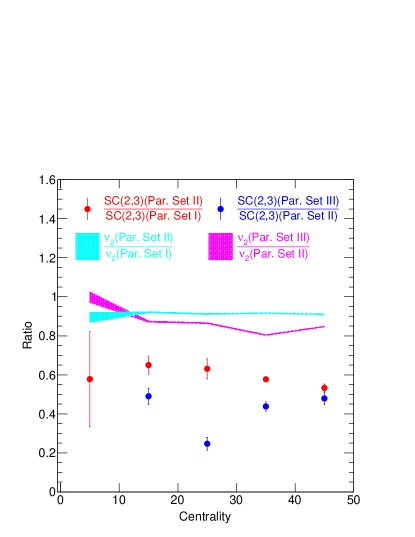
Figure 1: Ratios of $v_{2}\{4\}$ and $SC(2,3)$, with different hydro parameter sets, vs centrality in Au+Au collisions at $\sqrt{s_{NN}}$ = 200 GeV. The figure compares the effects of $\eta/s$ and $\zeta/s$ on $v_{2}\{4\}$ and $SC(2,3)$. The plotted results show ratios of $v_{2}\{4\}$ using bands and $SC(2,3)$ using markers. Certain data points with high uncertainty were excluded for clarity.

III.1.2 Six-particle asymmetric cumulants

Now, we present the results for $AC_{2,1}(m,n)$. In Fig.[2], we show the effect of shear viscosity on elliptic flow from the four-particle correlations and $AC_{2,1}(2,3)$. For $AC_{2,1}(2,3)$, we see a change of around 50% throughout the centrality range. We observe that the medium’s bulk viscosity also has a similar effect on these observables. Compared to the traditional flow observables, we see that these are more sensitive to the transport coefficients. Hence, these will put better constraints on the transport properties of the medium created in heavy-ion collisions.

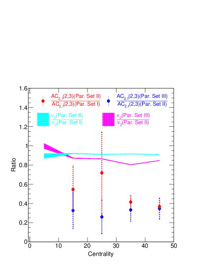
Figure 2: Ratios of $v_{2}\{4\}$ and $AC_{2,1}(2,3)$, with different hydro parameter sets, vs centrality in Au+Au collisions at $\sqrt{s_{NN}}$ = 200 GeV. The figure compares the effects of $\eta/s$ and $\zeta/s$ on $v_{2}\{4\}$ and $AC_{2,1}(2,3)$. The plotted results show ratios of $v_{2}\{4\}$ using bands and $AC_{2,1}(2,3)$ using markers. Certain data points with high uncertainty were excluded for clarity.

III.2 Centrality dependence of $SC(m,n)$ and $AC_{2,1}(m,n)$

III.2.1 Four-particle symmetric cumulants

Next, we compare the results from our simulations with the experimental measurements from RHIC. $SC(m,n)$ have been measured in previous studies from hydrodynamic and transport models [44, 43, 37, 45, 46, 47, 48], while $AC_{2,1}(m,n)$ have been measured in some transport models [46, 47]. Fig. [3] shows comparisons between the theory calculations for the symmetric cumulants $SC(2,3)$ and $SC(2,4)$ multiplied by $\langle N_{part}\rangle$ and the same measured by the STAR Collaboration [71]. The factor of $\langle N_{part}\rangle$ is multiplied to scale out the trivial dilution of correlation with the increase in the number of triplets. We are able to reproduce the qualitative variations with centrality. Here, we don’t aim to reproduce the experimental data because our aim is to check the sensitivity of these observables to the hydro transport coefficients. The comparison in Fig.[3] reflects that the correlation in initial spatial eccentricities and the following hydrodynamic evolution can capture the correlation among flow harmonics of different orders. Negative values of $SC(2,3)$ throughout the centrality range reveal the anti-correlation between $v_{2}$ and $v_{3}$. While as $SC(2,4)$ is positive for all centralities, indicating positive correlations between $v_{2}$ and $v_{4}$. Symmetric cumulants do not have contributions from non-flow effects, where non-flow refers to azimuthal correlations not related to the reaction plane orientation, like those from resonances, jets, quantum statistics, etc. This is verified by computing these observables for HIJING model, which includes only non-flow physics, for which these are consistently zero [35]. The model captures the variation of $SC(m,n)$ with the centrality. In central collisions, the model underestimates $SC(2,4)$, possibly due to inadequate fluctuations in the initial conditions or some shortcomings in the transport model since the nonlinear response in $v_{4}$ and $\varepsilon_{4}$ is sensitive to these effects. However, $SC(2,3)$ is better aligned with the data because the $v_{2}-v_{3}$ correlations mainly arise from the initial state $\varepsilon_{2}-\varepsilon_{3}$ correlations due to linear response in $v_{2}$ and $v_{3}$.

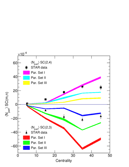
Figure 3: Symmetric cumulant vs centrality from four-particle correlations compared with STAR data [71] in Au+Au collisions at $\sqrt{s_{NN}}$ = 200 GeV. $SC(2,3)$ is consistently negative while as $SC(2,4)$ is consistently positive.

The normalized symmetric cumulants in Au+Au collisions at $\sqrt{s_{NN}}$ = 200 GeV, evaluated using the Monte Carlo Glauber model in coordinate space (using Eq.[11]), are presented in Fig.[4] and compared with $NSC(m,n)$ measured in momentum space. If only eccentricity drives $v_{n}$, then we can expect that the $NSC(m,n)$ in the final state would be equal to the $NSC(m,n)$ initial state. Fig.[4] shows that the initial anti-correlation between $\varepsilon_{2}$ and $\varepsilon_{3}$ is mainly responsible for the observed anti-correlation between $v_{2}$ and $v_{3}$. However, the correlation between $\varepsilon_{2}$ and $\varepsilon_{4}$ is smaller than the observed correlation between $v_{2}$ and $v_{4}$. The contribution to anisotropic flow $v_{4}$ not only comes from the linear response of the system to $\varepsilon_{4}$ but also has a contribution proportional to $\varepsilon_{2}^{2}$. As collisions become more peripheral, the difference between $NSC(2,4)$ in the final state and the initial state increases, likely due to $\varepsilon_{2}$ playing a more significant role in $v_{4}$. This has also been observed in Pb+Pb collisions at $\sqrt{s_{NN}}$ = 2.76 TeV by the ATLAS [72] and ALICE [39] experiments. The properties of the medium were suggested to affect the relative contribution of $\varepsilon_{2}$ in $v_{4}$ compared to $\varepsilon_{4}$ [73]. Therefore, $NSC(2,4)$ provides a probe into the medium properties.

$$\varepsilon_{n}e^{in\psi_{n}} = -\frac{\int r^{n}e^{in\phi}\rho\left(r,\phi\right)rdrd\phi}{\int r^{n}\rho\left(r,\phi\right)rdrd\phi},\hskip 2.84526ptn>2$$ (11)

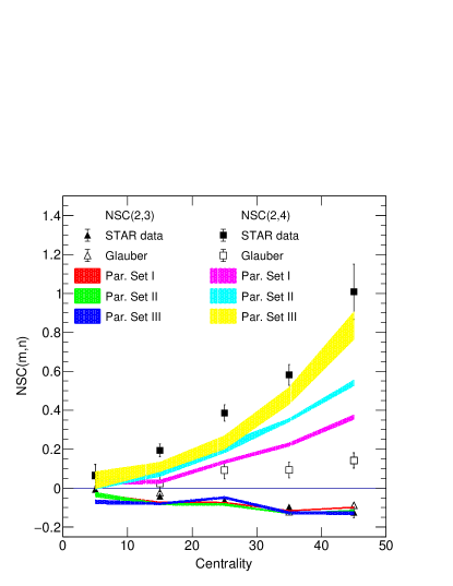
Figure 4: Normalized symmetric cumulant vs centrality from four-particle correlations compared with STAR data [71] in Au+Au collisions at $\sqrt{s_{NN}}$ = 200 GeV. $NSC(2,3)$ is consistently negative while as $NSC(2,4)$ is consistently positive.

III.2.2 Six-particle asymmetric cumulants

$AC_{2,1}(m,n)$ have measured by the ALICE collaboration for Pb+Pb collisions at $\sqrt{s_{NN}}=5.02\ TeV$ [49]. In Fig.[5], we should the centrality dependence of $AC_{2,1}(m,n)$ for Au+Au at $\sqrt{s_{NN}}=200\ GeV$. The trends are similar to the results by the ALICE collaboration. As for symmetric cumulants, negative values of $AC(2,3)$ throughout the centrality range reveal the anti-correlation between $v_{2}$ and $v_{3}$. While as $AC(2,4)$ is positive for all centralities, indicating positive correlations between $v_{2}$ and $v_{4}$. To check their sensitivity to the hydro transport coefficients, we compute these observables for the three sets of ensembles mentioned in Table  2. We observe that both $AC_{2,1}\{2,3\}$ and $AC_{2,1}\{2,4\}$ are suppressed by shear and bulk viscosities. For a clearer picture, the same results are plotted with a log scale for the y-axis in Fig.[6].

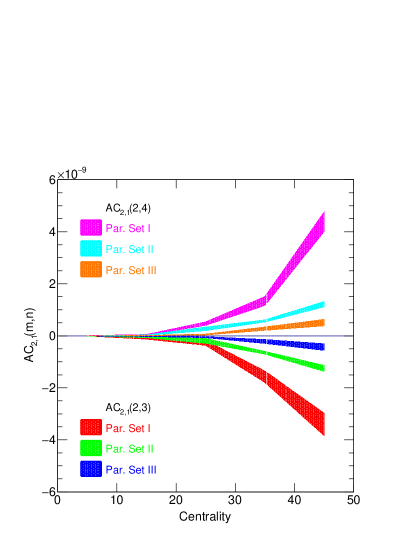
Figure 5: Asymmetric cumulant, $AC_{2,1}\{2,3\}$/$AC_{2,1}\{2,4\}$, vs centrality from six-particle correlations in Au+Au collisions at $\sqrt{s_{NN}}$ = 200 GeV.

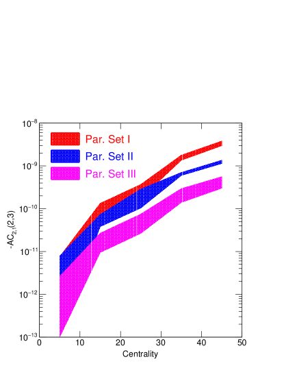
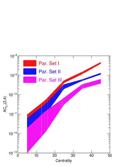
Figure 6: Asymmetric cumulants, -$AC_{2,1}\{2,3\}$ and $AC_{2,1}\{2,4\}$, vs centrality from six-particle correlations in Au+Au collisions at $\sqrt{s_{NN}}$ = 200 GeV. The upper panel shows $AC_{2,1}\{2,3\}$ multliplied by -1 to show the y-axis in log scale while as the lower panel shows $AC_{2,1}\{2,4\}$.

III.3 Conclusions

We have presented results for multi-particle correlation functions in heavy-ion collisions at top RHIC energy using a hybrid framework based on the Monte-Carlo Glauber model, MUSIC viscous hydrodynamics simulations, and the UrQMD hadronic cascade.

First, we adjusted the free parameters, such as shear and bulk viscosities, to accurately describe particle multiplicities, mean transverse momentum, and anisotropic flow. After that, we have discussed the impact of shear and bulk viscosities on traditional and novel observables.

We have studied correlators that measure the correlations between flow harmonics of varying orders, specifically four and six-particle correlations, including both symmetric and asymmetric cumulants as functions of centrality at midrapidity in Au+Au collisions at $\sqrt{s_{NN}}=200$ GeV. These new observables manifestly satisfy all mathematical properties of cumulants in the basis in which they are expressed. This new approach allows for the separation of non-flow and flow contributions and provides initial insights into how the combinatorial background contributes to flow measurements using correlation techniques.

The hybrid framework that we have used yields good agreement with the majority of the latest multi-particle observables from RHIC. In addition, the hadronic afterburner plays an essential role in describing the data collected at RHIC [44]. Study based on HIJING demonstrated that these new observables are robust against systematic biases due to non-flow correlations [43].

Compared to traditional flow observables, the novel observables are more sensitive to transport coefficients, resulting in better constraints on the transport properties of the medium created in heavy-ion collisions. We observed anti-correlation between event-by-event fluctuations of $v_{2}$ and $v_{3}$, while the event-by-event fluctuations of $v_{2}$ and $v_{4}$ are found to be positively correlated. The observed anti-correlation between $v_{2}$ and $v_{3}$ appears to be described by the initial-stage anti-correlation between $\varepsilon_{2}$ and $\varepsilon_{3}$, which supports the idea of linearity between $\varepsilon_{n}$ and $v_{n}$ [23]. The hydrodynamic response suggests that the final state fluctuation originates from the initial state. However, including the nonlinear hydrodynamic response of the medium is necessary to reproduce the measured correlation between $v_{2}$ and $v_{4}$, as the initial-stage correlation alone is insufficient. Therefore, we can gain new knowledge regarding the initial conditions and properties of QGP in high-energy nuclear collisions from these higher-order observables. Symmetric and asymmetric cumulants of flow amplitudes can be used directly to constrain the multivariate probability density function of flow fluctuations since its functional form can be reconstructed only from its true moments or cumulants.

III.4 Acknowledgements

We would like to acknowledge Tribhuban Parida for fruitful discussions and providing us the computational setup.

References

- Collins and Perry [1975] J. C. Collins and M. J. Perry, Superdense Matter: Neutrons Or Asymptotically Free Quarks?, Phys. Rev. Lett. 34, 1353 (1975).
- Shuryak [2005] E. V. Shuryak, What RHIC experiments and theory tell us about properties of quark-gluon plasma?, Nucl. Phys. A 750, 64 (2005), arXiv:hep-ph/0405066 .
- Busza et al. [2018] W. Busza, K. Rajagopal, and W. van der Schee, Heavy Ion Collisions: The Big Picture, and the Big Questions, Ann. Rev. Nucl. Part. Sci. 68, 339 (2018), arXiv:1802.04801 [hep-ph] .
- Ackermann et al. [2001] K. H. Ackermann et al. (STAR), Elliptic flow in Au + Au collisions at (S(NN))**(1/2) = 130 GeV, Phys. Rev. Lett. 86, 402 (2001), arXiv:nucl-ex/0009011 .
- Abelev et al. [2007] B. I. Abelev et al. (STAR), Partonic flow and phi-meson production in Au + Au collisions at s(NN)**(1/2) = 200-GeV, Phys. Rev. Lett. 99, 112301 (2007), arXiv:nucl-ex/0703033 .
- Adcox et al. [2005] K. Adcox et al. (PHENIX), Formation of dense partonic matter in relativistic nucleus-nucleus collisions at RHIC: Experimental evaluation by the PHENIX collaboration, Nucl. Phys. A 757, 184 (2005), arXiv:nucl-ex/0410003 .
- Heinz and Snellings [2013] U. Heinz and R. Snellings, Collective flow and viscosity in relativistic heavy-ion collisions, Ann. Rev. Nucl. Part. Sci. 63, 123 (2013), arXiv:1301.2826 [nucl-th] .
- Braun-Munzinger et al. [2016] P. Braun-Munzinger, V. Koch, T. Schäfer, and J. Stachel, Properties of hot and dense matter from relativistic heavy ion collisions, Phys. Rept. 621, 76 (2016), arXiv:1510.00442 [nucl-th] .
- Voloshin and Zhang [1996] S. Voloshin and Y. Zhang, Flow study in relativistic nuclear collisions by Fourier expansion of Azimuthal particle distributions, Z. Phys. C 70, 665 (1996), arXiv:hep-ph/9407282 .
- Ollitrault [1992] J.-Y. Ollitrault, Anisotropy as a signature of transverse collective flow, Phys. Rev. D 46, 229 (1992).
- Bass et al. [1999] S. A. Bass, M. Gyulassy, H. Stoecker, and W. Greiner, Signatures of quark gluon plasma formation in high-energy heavy ion collisions: A Critical review, J. Phys. G 25, R1 (1999), arXiv:hep-ph/9810281 .
- Voloshin et al. [2010] S. A. Voloshin, A. M. Poskanzer, and R. Snellings, Collective phenomena in non-central nuclear collisions, Landolt-Bornstein 23, 293 (2010), arXiv:0809.2949 [nucl-ex] .
- Voloshin and Poskanzer [2000] S. A. Voloshin and A. M. Poskanzer, The Physics of the centrality dependence of elliptic flow, Phys. Lett. B 474, 27 (2000), arXiv:nucl-th/9906075 .
- Ivanov and Soldatov [2015] Y. B. Ivanov and A. A. Soldatov, Elliptic Flow in Heavy-Ion Collisions at Energies 2.7-39 GeV, Phys. Rev. C 91, 024914 (2015), arXiv:1401.2265 [nucl-th] .
- Adams et al. [2005] J. Adams et al. (STAR), Azimuthal anisotropy in Au+Au collisions at s(NN)**(1/2) = 200-GeV, Phys. Rev. C 72, 014904 (2005), arXiv:nucl-ex/0409033 .
- Adler et al. [2001] C. Adler et al. (STAR), Identified particle elliptic flow in Au + Au collisions at s(NN)**(1/2) = 130-GeV, Phys. Rev. Lett. 87, 182301 (2001), arXiv:nucl-ex/0107003 .
- Aamodt et al. [2010] K. Aamodt et al. (ALICE), Elliptic flow of charged particles in Pb-Pb collisions at 2.76 TeV, Phys. Rev. Lett. 105, 252302 (2010), arXiv:1011.3914 [nucl-ex] .
- Sorge [1999] H. Sorge, Highly sensitive centrality dependence of elliptic flow: A novel signature of the phase transition in QCD, Phys. Rev. Lett. 82, 2048 (1999), arXiv:nucl-th/9812057 .
- Adamczyk et al. [2013] L. Adamczyk et al. (STAR), Third Harmonic Flow of Charged Particles in Au+Au Collisions at sqrtsNN = 200 GeV, Phys. Rev. C 88, 014904 (2013), arXiv:1301.2187 [nucl-ex] .
- Solanki et al. [2013] D. Solanki, P. Sorensen, S. Basu, R. Raniwala, and T. K. Nayak, Beam energy dependence of Elliptic and Triangular flow with the AMPT model, Phys. Lett. B 720, 352 (2013), arXiv:1210.0512 [nucl-ex] .
- Adam et al. [2016a] J. Adam et al. (ALICE), Higher harmonic flow coefficients of identified hadrons in Pb-Pb collisions at = 2.76 TeV, JHEP 09, 164, arXiv:1606.06057 [nucl-ex] .
- Heinz et al. [2013] U. Heinz, Z. Qiu, and C. Shen, Fluctuating flow angles and anisotropic flow measurements, Phys. Rev. C 87, 034913 (2013), arXiv:1302.3535 [nucl-th] .
- Alver and Roland [2010] B. Alver and G. Roland, Collision geometry fluctuations and triangular flow in heavy-ion collisions, Phys. Rev. C 81, 054905 (2010), [Erratum: Phys.Rev.C 82, 039903 (2010)], arXiv:1003.0194 [nucl-th] .
- Parkkila et al. [2021] J. E. Parkkila, A. Onnerstad, and D. J. Kim, Bayesian estimation of the specific shear and bulk viscosity of the quark-gluon plasma with additional flow harmonic observables, Phys. Rev. C 104, 054904 (2021), arXiv:2106.05019 [hep-ph] .
- Retinskaya et al. [2014] E. Retinskaya, M. Luzum, and J.-Y. Ollitrault, Constraining models of initial state with and data from LHC and RHIC, Nucl. Phys. A 926, 152 (2014), arXiv:1401.3241 [nucl-th] .
- Shen and Heinz [2012] C. Shen and U. Heinz, Collision Energy Dependence of Viscous Hydrodynamic Flow in Relativistic Heavy-Ion Collisions, Phys. Rev. C 85, 054902 (2012), [Erratum: Phys.Rev.C 86, 049903 (2012)], arXiv:1202.6620 [nucl-th] .
- Teaney [2003] D. Teaney, The Effects of viscosity on spectra, elliptic flow, and HBT radii, Phys. Rev. C 68, 034913 (2003), arXiv:nucl-th/0301099 .
- Shen et al. [2011] C. Shen, S. A. Bass, T. Hirano, P. Huovinen, Z. Qiu, H. Song, and U. Heinz, The QGP shear viscosity: Elusive goal or just around the corner?, J. Phys. G 38, 124045 (2011), arXiv:1106.6350 [nucl-th] .
- Wang et al. [1991] S. Wang, Y. Z. Jiang, Y. M. Liu, D. Keane, D. Beavis, S. Y. Chu, S. Y. Fung, M. Vient, C. Hartnack, and H. Stoecker, Measurement of collective flow in heavy ion collisions using particle pair correlations, Phys. Rev. C 44, 1091 (1991).
- Jiang et al. [1992] J. Jiang et al., High order collective flow correlations in heavy ion collisions, Phys. Rev. Lett. 68, 2739 (1992).
- Bhalerao et al. [2011] R. S. Bhalerao, M. Luzum, and J.-Y. Ollitrault, Determining initial-state fluctuations from flow measurements in heavy-ion collisions, Phys. Rev. C 84, 034910 (2011), arXiv:1104.4740 [nucl-th] .
- Borghini et al. [2001a] N. Borghini, P. M. Dinh, and J.-Y. Ollitrault, New method for measuring azimuthal distributions in nucleus-nucleus collisions, Phys. Rev. C 63, 054906 (2001a).
- Borghini et al. [2001b] N. Borghini, P. M. Dinh, and J.-Y. Ollitrault, Flow analysis from multiparticle azimuthal correlations, Phys. Rev. C 64, 054901 (2001b).
- Bilandzic et al. [2014a] A. Bilandzic, C. H. Christensen, K. Gulbrandsen, A. Hansen, and Y. Zhou, Generic framework for anisotropic flow analyses with multiparticle azimuthal correlations, Phys. Rev. C 89, 064904 (2014a).
- Bilandzic et al. [2022] A. Bilandzic, M. Lesch, C. Mordasini, and S. F. Taghavi, Multivariate cumulants in flow analyses: The next generation, Phys. Rev. C 105, 024912 (2022).
- Bilandzic et al. [2014b] A. Bilandzic, C. H. Christensen, K. Gulbrandsen, A. Hansen, and Y. Zhou, Generic framework for anisotropic flow analyses with multiparticle azimuthal correlations, Phys. Rev. C 89, 064904 (2014b), arXiv:1312.3572 [nucl-ex] .
- Taghavi [2021] S. F. Taghavi, A Fourier-cumulant analysis for multiharmonic flow fluctuation: by employing a multidimensional generating function approach, Eur. Phys. J. C 81, 652 (2021), arXiv:2005.04742 [nucl-th] .
- Adam et al. [2018a] J. Adam et al. (STAR), Correlation measurements between flow harmonics in au+au collisions at rhic, Physics Letters B 783, 459 (2018a).
- Adam et al. [2016b] J. Adam et al. (ALICE), Correlated event-by-event fluctuations of flow harmonics in Pb-Pb collisions at TeV, Phys. Rev. Lett. 117, 182301 (2016b), arXiv:1604.07663 [nucl-ex] .
- Niemi et al. [2013] H. Niemi, G. S. Denicol, H. Holopainen, and P. Huovinen, Event-by-event distributions of azimuthal asymmetries in ultrarelativistic heavy-ion collisions, Phys. Rev. C 87, 054901 (2013).
- Nasim [2017] M. Nasim, Systematic study of symmetric cumulants at = 200 GeV in Au+Au collision using transport approach, Phys. Rev. C 95, 034905 (2017), arXiv:1612.01066 [nucl-ex] .
- Parkkila et al. [2022] J. E. Parkkila, A. Onnerstad, S. F. Taghavi, C. Mordasini, A. Bilandzic, M. Virta, and D. J. Kim, New constraints for QCD matter from improved Bayesian parameter estimation in heavy-ion collisions at LHC, Phys. Lett. B 835, 137485 (2022), arXiv:2111.08145 [hep-ph] .
- Mordasini et al. [2020] C. Mordasini, A. Bilandzic, D. Karakoç, and S. F. Taghavi, Higher order Symmetric Cumulants, Phys. Rev. C 102, 024907 (2020), arXiv:1901.06968 [nucl-ex] .
- Schenke et al. [2019] B. Schenke, C. Shen, and P. Tribedy, Multi-particle and charge-dependent azimuthal correlations in heavy-ion collisions at the Relativistic Heavy-Ion Collider, Phys. Rev. C 99, 044908 (2019), arXiv:1901.04378 [nucl-th] .
- Hirvonen et al. [2022] H. Hirvonen, K. J. Eskola, and H. Niemi, Flow correlations from a hydrodynamics model with dynamical freeze-out and initial conditions based on perturbative QCD and saturation, Phys. Rev. C 106, 044913 (2022), arXiv:2206.15207 [hep-ph] .
- Magdy [2023] N. Magdy, Characterizing initial- and final-state effects of relativistic nuclear collisions, Phys. Rev. C 107, 024905 (2023), arXiv:2210.14091 [nucl-th] .
- Magdy [2024] N. Magdy, Characterizing the initial- and final-state effects in isobaric collisions at energies available at the BNL Relativistic Heavy Ion Collider, Phys. Rev. C 109, 024906 (2024), arXiv:2401.04083 [nucl-th] .
- Gardim et al. [2017] F. G. Gardim, F. Grassi, M. Luzum, and J. Noronha-Hostler, Hydrodynamic Predictions for Mixed Harmonic Correlations in 200 GeV Au+Au Collisions, Phys. Rev. C 95, 034901 (2017), arXiv:1608.02982 [nucl-th] .
- Acharya et al. [2023] S. Acharya et al. (ALICE), Higher-order correlations between different moments of two flow amplitudes in Pb-Pb collisions at sNN=5.02 TeV, Phys. Rev. C 108, 055203 (2023), arXiv:2303.13414 [nucl-ex] .
- Aaboud et al. [2019] M. Aaboud et al. (ATLAS), Correlated long-range mixed-harmonic fluctuations measured in , +Pb and low-multiplicity Pb+Pb collisions with the ATLAS detector, Phys. Lett. B 789, 444 (2019), arXiv:1807.02012 [nucl-ex] .
- Ortiz [2019] A. Ortiz (ALICE, ATLAS, CMS, LHCb), Particle production and flow-like effects in small systems, PoS LHCP2019, 091 (2019), arXiv:1909.03937 [hep-ex] .
- Sirunyan et al. [2021] A. M. Sirunyan et al. (CMS), Correlations of azimuthal anisotropy Fourier harmonics with subevent cumulants in collisions at 8.16TeV, Phys. Rev. C 103, 014902 (2021), arXiv:1905.09935 [hep-ex] .
- Acharya et al. [2021] S. Acharya et al. (ALICE), Measurements of mixed harmonic cumulants in Pb–Pb collisions at = 5.02 TeV, Phys. Lett. B 818, 136354 (2021), arXiv:2102.12180 [nucl-ex] .
- Shou et al. [2015] Q. Y. Shou, Y. G. Ma, P. Sorensen, A. H. Tang, F. Videbæk, and H. Wang, Parameterization of Deformed Nuclei for Glauber Modeling in Relativistic Heavy Ion Collisions, Phys. Lett. B 749, 215 (2015), arXiv:1409.8375 [nucl-th] .
- Schenke et al. [2010] B. Schenke, S. Jeon, and C. Gale, (3+1)D hydrodynamic simulation of relativistic heavy-ion collisions, Phys. Rev. C 82, 014903 (2010), arXiv:1004.1408 [hep-ph] .
- Schenke et al. [2011] B. Schenke, S. Jeon, and C. Gale, Elliptic and triangular flow in event-by-event (3+1)D viscous hydrodynamics, Phys. Rev. Lett. 106, 042301 (2011), arXiv:1009.3244 [hep-ph] .
- Paquet et al. [2016] J.-F. Paquet, C. Shen, G. S. Denicol, M. Luzum, B. Schenke, S. Jeon, and C. Gale, Production of photons in relativistic heavy-ion collisions, Phys. Rev. C 93, 044906 (2016), arXiv:1509.06738 [hep-ph] .
- Huovinen and Petersen [2012] P. Huovinen and H. Petersen, Particlization in hybrid models, Eur. Phys. J. A 48, 171 (2012), arXiv:1206.3371 [nucl-th] .
- Denicol et al. [2009] G. S. Denicol, T. Kodama, T. Koide, and P. Mota, Bulk viscosity effects on elliptic flow, Nucl. Phys. A 830, 729C (2009), arXiv:0907.4269 [hep-ph] .
- Monnai et al. [2019] A. Monnai, B. Schenke, and C. Shen, Equation of state at finite densities for QCD matter in nuclear collisions, Phys. Rev. C 100, 024907 (2019), arXiv:1902.05095 [nucl-th] .
- Bazavov et al. [2014] A. Bazavov et al. (HotQCD), Equation of state in ( 2+1 )-flavor QCD, Phys. Rev. D 90, 094503 (2014), arXiv:1407.6387 [hep-lat] .
- Bazavov et al. [2012] A. Bazavov et al. (HotQCD), Fluctuations and Correlations of net baryon number, electric charge, and strangeness: A comparison of lattice QCD results with the hadron resonance gas model, Phys. Rev. D 86, 034509 (2012), arXiv:1203.0784 [hep-lat] .
- Ding et al. [2015] H. T. Ding, S. Mukherjee, H. Ohno, P. Petreczky, and H. P. Schadler, Diagonal and off-diagonal quark number susceptibilities at high temperatures, Phys. Rev. D 92, 074043 (2015), arXiv:1507.06637 [hep-lat] .
- Moreland and Soltz [2016] J. S. Moreland and R. A. Soltz, Hydrodynamic simulations of relativistic heavy-ion collisions with different lattice quantum chromodynamics calculations of the equation of state, Phys. Rev. C 93, 044913 (2016), arXiv:1512.02189 [nucl-th] .
- Shen et al. [2016] C. Shen, Z. Qiu, H. Song, J. Bernhard, S. Bass, and U. Heinz, The iEBE-VISHNU code package for relativistic heavy-ion collisions, Comput. Phys. Commun. 199, 61 (2016), arXiv:1409.8164 [nucl-th] .
- [66] The iSS code packge can be downloaded from GitHub.
- Bleicher et al. [1999] M. Bleicher et al., Relativistic hadron hadron collisions in the ultrarelativistic quantum molecular dynamics model, J. Phys. G 25, 1859 (1999), arXiv:hep-ph/9909407 .
- Bass et al. [1998] S. A. Bass et al., Microscopic models for ultrarelativistic heavy ion collisions, Prog. Part. Nucl. Phys. 41, 255 (1998), arXiv:nucl-th/9803035 .
- Abelev et al. [2009] B. I. Abelev et al. (STAR), Systematic Measurements of Identified Particle Spectra in Au and Au+Au Collisions from STAR, Phys. Rev. C 79, 034909 (2009), arXiv:0808.2041 [nucl-ex] .
- Adare et al. [2011] A. Adare et al. (PHENIX), Measurements of Higher-Order Flow Harmonics in Au+Au Collisions at GeV, Phys. Rev. Lett. 107, 252301 (2011), arXiv:1105.3928 [nucl-ex] .
- Adam et al. [2018b] J. Adam et al. (STAR), Correlation Measurements Between Flow Harmonics in Au+Au Collisions at RHIC, Phys. Lett. B 783, 459 (2018b), arXiv:1803.03876 [nucl-ex] .
- Aad et al. [2015] G. Aad et al. (ATLAS), Measurement of the correlation between flow harmonics of different order in lead-lead collisions at =2.76 TeV with the ATLAS detector, Phys. Rev. C 92, 034903 (2015), arXiv:1504.01289 [hep-ex] .
- Teaney and Yan [2012] D. Teaney and L. Yan, Non linearities in the harmonic spectrum of heavy ion collisions with ideal and viscous hydrodynamics, Phys. Rev. C 86, 044908 (2012), arXiv:1206.1905 [nucl-th] .