A second-order semi-Lagrangian exponential scheme with application to the shallow-water equations on the rotating sphere

Abstract

In this work, we study and extend a class of semi-Lagrangian exponential methods, which combine exponential time integration techniques, suitable for integrating stiff linear terms, with a semi-Lagrangian treatment of nonlinear advection terms. Partial differential equations involving both processes arise for instance in atmospheric circulation models. Through a truncation error analysis, we first show that previously formulated semi-Lagrangian exponential schemes are limited to first-order accuracy due to the discretization of the linear term; we then formulate a new discretization leading to a second-order accurate method. Also, a detailed stability study, both considering a linear stability analysis and an empirical simulation-based one, is conducted to compare several Eulerian and semi-Lagrangian exponential schemes, as well as a well-established semi-Lagrangian semi-implicit method, which is used in operational atmospheric models. Numerical simulations of the shallow-water equations on the rotating sphere, considering standard and challenging benchmark test cases, are performed to assess the orders of convergence, stability properties, and computational cost of each method. The proposed second-order semi-Lagrangian exponential method was shown to be more stable and accurate than the previously formulated schemes of the same class at the expense of larger wall-clock times; however, the method is more stable and has a similar cost compared to the well-established semi-Lagrangian semi-implicit; therefore, it is a competitive candidate for potential operational applications in atmospheric circulation modeling.

65M12, 65M22, 76U60

1 Introduction

Exponential integration methods are a large class of time stepping schemes that have raised increasing interest for the integration of time-dependent partial differential equations containing stiff linear operators, since they allow to integrate exactly (or at least very accurately) the linear terms of the governing equations, thus overcoming stability constraints related to their stiffness [22, 15]. These methods require the evaluation of matrix exponentials, which is a main challenge for their efficient implementation. The recent development of accurate and efficient linear algebra methods has directly contributed to the development and popularization of exponential integration schemes [22], which have been increasingly seen as viable alternatives to overcome Courant-Friedrichs-Lewy (CFL)-related time step limitations usually found in complex fluid dynamics problems such as in atmospheric modeling [12].

The development of exponential integration methods goes back to 1960, by [5], in which the variation of constants formula was used to derive the scheme, leading to the family of Exponential Time Differencing (ETD) methods. An alternative approach, proposed by [18], consists of defining a change of variables leading to a differential equation in which the linear operator appears only as arguments of exponential functions, a class of exponential schemes known as Integrating Factor (IF) methods. Both classes are derived considering a partition of the governing equations into linear and nonlinear terms. A third well-known class of exponential schemes is composed of the exponential Rosenbrock methods [14], which are derived from a linearization of the full time evolution operator, thus requiring the computation of its Jacobian. Since then, several ETD, IF and Rosenbrock exponential methods have been proposed and applied in various contexts, as well as novel classes of exponential schemes. Detailed reviews on exponential integration methods can be found, e.g., in [22, 15]. These methods have been studied and applied in a very diverse range of contexts. In particular, several recent works have focused on geophysical fluid dynamics, in particular atmospheric circulation models, which is the application domain targeted in this work. [1, 6] assessed good stability properties and improved accuracy of Rosenbrock-type exponential schemes, compared to more traditional semi-implicit methods, when applied to the shallow-water equations (SWE) on the rotating sphere, but highlighted the need for more efficient approaches for computing the exponential of large matrices. Similar conclusions have been drawn by [2] comparing various time integration schemes in the context of the one-dimensional SWE. The challenge of improving the exponential computation has been tackled by [12, 20, 38]. Applications to more complex, three-dimensional atmospheric models have been investigated by [27, 26], with stable and accurate integration of both slow and fast atmospheric dynamics. Finally, methods considering rational approximations to the exponential functions, which lead to parallel-in-time methods, have been investigated for the SWE on the rotating sphere by [30, 31].

More recently, [24] proposed a class of semi-Lagrangian Runge-Kutta-type ETD schemes (SL-ETDRK) to tackle advective PDEs, inspired by the Eulerian ETDRK methods proposed by [7]. Semi-Lagrangian schemes, which follow the trajectories of particles along each time step instead of relying on fixed spatial grids as in Eulerian approaches, are popular methods in atmospheric modeling due to their improved stability properties. This improved stability was indeed verified for the proposed SL-ETDRK schemes in [24], through the numerical simulation of the SWE on the bi-periodic plane with a spectral discretization in space. A semi-Lagrangian exponential method has also been developed by [33], based on the Rosenbrock exponential approach, leading to a second-order scheme whose accuracy was confirmed on numerical tests of the SWE on the rotating sphere considering a cubed grid discretization.

This work proposes a better analytical understanding of convergence and stability properties of the SL-ETDRK schemes, as well as improvements for these methods. Indeed, although these methods have been derived analogously to their respective Eulerian counterparts ETD1RK and ETD2RK (respectively first- and second-order accurate) [7], the expected second-order convergence of SL-ETD2RK is not verified in practice. The numerical simulations presented by [24] reveal that both SL-ETD1RK and SL-ETD2RK are first-order accurate, but the reasons for that were not clear. Here, we prove that the observed first-order accuracy of SL-ETD2RK is due to the discretization of the linear term, which involves both an exponential operator and a spatial interpolation coming from the semi-Lagrangian approach. This issue is naturally absent in Eulerian schemes, in which the exponential integrates exactly the linear term. Then, we propose an alternative discretization, consisting of a splitting of the exponential operator, and prove that it leads indeed to second-order accuracy. We also conduct a detailed analytical stability study of both Eulerian and semi-Lagrangian ETDRK schemes, as well as the popular semi-Lagrangian semi-implicit SETTLS method [16] used in operational atmospheric models; we show in particular that standard linear stability analyses are not able to provide concluding insights on the stability of semi-Lagrangian exponential schemes due to a lack of commutation between exponential and interpolation operators; therefore, we conduct an empirical simulation-based stability study following a procedure described by [25]. Finally, we perform numerical experiments for the assessment of convergence and stability of the proposed improved schemes.

In terms of application, our focus here is on the use of semi-Lagrangian exponential methods in the context of atmospheric modeling. Atmospheric circulation models are characterized by a vast range of waves propagating at different speeds, with the fast ones being responsible for often severe stability constraints, which has motivated the development of various discretization methods searching to establish a good trade-off between stability, accuracy, and computational cost [39]; therefore, combining the semi-Lagrangian and exponential approaches could better handle both advection processes and the stiffness of the linear terms. In particular, we expect semi-Lagrangian exponential methods to be more stable than Eulerian exponential ones, and more accurate than traditional semi-Lagrangian schemes (at least when stiff, linear processes have relatively important magnitude), such that good compromises between computational cost and accuracy could be obtained. We consider, for the numerical experiments and stability analyses conducted here, the SWE on the rotating sphere, using challenging benchmark test cases commonly used in atmospheric modeling research; thus, this work not only analyses and improves the semi-Lagrangian exponential methods proposed by [24], but it also extends their application domain since [24] focused on the SWE on the plane. Finally, we also compare the exponential semi-Lagrangian scheme to the well-established SL-SI-SETTLS, in order to assess the competitiveness of semi-Lagrangian exponential methods.

This paper is organized as follows: the shallow-water equations on the rotating sphere are introduced in Section 2; the time integrators considered in this work (the Eulerian ETDRK schemes by [7], the SL-ETDRK schemes by [24] and SL-SI-SETTLS by [16]) are presented in Section 3; a truncation error analysis indicating the sources of the first-order accuracy of the SL-ETD2RK scheme is developed in Section 4; an effectively second-order accurate semi-Lagrangian exponential method is proposed in Section 5, as well as its truncation error and computational complexity analyses; a detailed linear stability study comparing the various schemes considered in this work is conducted in Section 6; numerical simulations of the SWE on the rotating sphere are performed in Section 7 in order to assess and compare stability, convergence and computational cost properties; and conclusions are presented in Section 8.

2 The shallow-water equations on the rotating sphere

The shallow-water equations on the rotating sphere are a popular two-dimensional model in the early stages of atmospheric circulation research since it is simplified w.r.t. to more complete, three-dimensional equations but still contains most of the challenges related to the spatial discretization of atmospheric models. Therefore, it allows an easier but insightful study of spatial and temporal discretization schemes for atmospheric models [40]. The equations read

(1) $$\frac{\partial}{\partial t}\boldsymbol{U} =\boldsymbol{L}_{\boldsymbol{G}}(\boldsymbol{U})+\boldsymbol{L}_{\boldsymbol{C}}(\boldsymbol{U})+\boldsymbol{N}_{\boldsymbol{A}}(\boldsymbol{U})+\boldsymbol{N}_{\boldsymbol{R}}(\boldsymbol{U})+\boldsymbol{L}_{\nu}(\boldsymbol{U})+\boldsymbol{b},$$

where the solution vector $\boldsymbol{U}=\left(\Phi,\ \xi,\ \delta\right)^{T}$ contains the geopotential $\Phi=\overline{\Phi}+\Phi^{\prime}=gh$, vorticity $\xi:=\boldsymbol{z}\cdot(\nabla\times\boldsymbol{V})$ and divergence $\delta:=\nabla\cdot\boldsymbol{V}$ fields. $\Phi$, $\xi$ and $\delta$ are functions of $(\lambda,\mu,t)$, where $\lambda$ is the longitude, $\mu=\sin(\theta)$, $\theta$ is the latitude and $t$ is the time. $g$ denotes the gravitational acceleration, $h$ is the fluid depth, $\overline{\Phi}$ and $\Phi^{\prime}$ are respectively the mean geopotential and the geopotential perturbation, $\boldsymbol{V}:=\left(u,\ v\right)^{T}$ is the horizontal velocity field and $\boldsymbol{z}$ is the unit vector in the vertical direction. The RHS of (1) is decomposed as a sum of linear and nonlinear terms accounting for different physical processes: $\boldsymbol{L}_{\boldsymbol{G}}$ accounts for linear processes related to the gravitation; $\boldsymbol{L}_{\boldsymbol{C}}$ contains linear rotation-related phenomena, described by the Coriolis parameter $f=2\Omega\sin\theta$, where $\Omega$ is the Earth’s angular velocity; $\boldsymbol{N}_{\boldsymbol{A}}$ is the nonlinear advection term, $\boldsymbol{N}_{\boldsymbol{R}}$ contains the remaining nonlinear terms, $\boldsymbol{L}_{\nu}(\boldsymbol{U})$ is a linear term accounting for an artificial (hyper-)viscosity of order $q$ and coefficient $\nu\geq 0$, with $q$ even, and $\boldsymbol{b}$ is related to the topography field $b$. These terms are given by

(2) $$\begin{gathered}\boldsymbol{L}_{\boldsymbol{G}}(\boldsymbol{U})=\left(\begin{array}[]{c c c}0&0&-\overline{\Phi}\\ 0&0&0\\ -\nabla^{2}&0&0\end{array}\right)\boldsymbol{U},\qquad\boldsymbol{L}_{\boldsymbol{C}}(\boldsymbol{U})=\left(\begin{array}[]{c}0\\ -\nabla\cdot(f\boldsymbol{V})\\ \boldsymbol{z}\cdot\nabla\times(f\boldsymbol{V})\end{array}\right)\\ \boldsymbol{N}_{\boldsymbol{A}}(\boldsymbol{U})=\left(\begin{array}[]{c}-\boldsymbol{V}\cdot\nabla\Phi\\ -\nabla\cdot(\xi\boldsymbol{V})\\ -\nabla^{2}\left(\frac{\boldsymbol{V}\cdot\boldsymbol{V}}{2}\right)+\boldsymbol{z}\cdot\nabla\times(\xi\boldsymbol{V})\end{array}\right),\qquad\boldsymbol{N}_{\boldsymbol{R}}(\boldsymbol{U})=\left(\begin{array}[]{c}-\Phi^{\prime}\delta\\ 0\\ 0\end{array}\right),\\ \boldsymbol{L}_{\nu}(\boldsymbol{U})=(-1)^{\frac{q}{2}+1}\nu\left(\begin{array}[]{c}\nabla^{q}\Phi^{\prime}\\ \nabla^{q}\xi\\ \nabla^{q}\delta\end{array}\right),\qquad\boldsymbol{b}=\left(\begin{array}[]{c}0\\ 0\\ -g\nabla^{2}b\end{array}\right).\end{gathered}$$

2.1 Spectral discretization

In this work, the spatial dimension is discretized considering a spectral approach using spherical harmonics, which is briefly described below. Details can be found in [9]. Let $Y_{m,n}$ denote the spherical harmonic function of zonal and total wavenumbers $m$ and $n$, respectively. The spherical harmonics expansion of a given smooth field $\psi$ reads

(3) $$\psi(\lambda,\mu,t)=\sum_{m=-\infty}^{\infty}\sum_{n=|m|}^{\infty}\psi_{m,n}(t)Y_{m,n}(\lambda,\mu)$$

where $\psi_{m,n}$ is the expansion coefficient corresponding to the wavenumber pair $(m,n)$. We consider a triangular truncation with resolution $M$:

(4) $$\psi(\lambda,\mu,t)=\sum_{m=-M}^{M}\sum_{n=|m|}^{M}\psi_{m,n}(t)Y_{m,n}(\lambda,\mu)$$

As described in the next section, the use of a spectral discretization based on spherical harmonics, combined with a proper arrangement of the terms of the governing equations, is essential for ensuring an efficient computation of matrix exponentials in both Eulerian and semi-Lagrangian exponential methods.

3 Time integrators

We present in this section the time stepping schemes considered in the work. We begin by briefly presenting the Eulerian exponential integration methods ETD1RK and ETD2RK [7], on which their semi-Lagrangian versions are based. Then, as an introduction to semi-Lagrangian schemes, we present the semi-Lagrangian semi-implicit SETTLS [16], which we will also compare in the numerical experiments. Finally, we present the semi-Lagrangian exponential schemes proposed by [24]. As explained below, we propose a modification to the name of this last class of methods in order to take into account their actual order of convergence.

3.1 Eulerian Runge-Kutta-type exponential integration methods (ETDRK)

Exponential Time Differencing (ETD) schemes are a class of exponential integration methods to solve time-dependent problems of the form

(5) $$\frac{d\boldsymbol{U}}{dt}=\boldsymbol{L}\boldsymbol{U}+\boldsymbol{N}(\boldsymbol{U}),\qquad\boldsymbol{U}(t=0)=\boldsymbol{U}_{0},$$

which are obtained, e.g., from a spatial discretization of a PDE, where $\boldsymbol{U}\in\mathbb{R}^{N}$, $\boldsymbol{L}\in\mathbb{R}^{N\times N}$ is a linear operator and $\boldsymbol{N}:\mathbb{R}^{N}\rightarrow\mathbb{R}^{N}$ is a nonlinear function. As a common feature, exponential methods integrate the linear term $\boldsymbol{L}\boldsymbol{U}$ very accurately (or exactly, down to machine precision, if the exponential terms can be evaluated exactly), by writing its evolution using the exponential of the linear operator, whereas an approximation is proposed to compute the nonlinear term. In the following paragraphs, we briefly describe the main ideas behind exponential methods, more specifically concerning the schemes considered in this work, namely ETDRK [7] and SL-ETDRK [24]. We refer the reader to [7, 15] for further details on exponential integration methods and their derivation.

The exact solution of (5) at time $t_{n+1}=t_{n}+\Delta t$, integrated from $\boldsymbol{U}(t_{n})$, reads

(6) $$\boldsymbol{U}(t_{n+1})=e^{\Delta t\boldsymbol{L}}\boldsymbol{U}(t_{n})+\int_{t_{n}}^{t_{n+1}}e^{-(s-t_{n})\boldsymbol{L}}\boldsymbol{N}(\boldsymbol{U}(s))ds.$$

The first term in (6) is the exact integration of the linear term. Different exponential methods can be formulated proposing different approximations to the integral containing the evolution of the nonlinear term.

In particular, ETDRK methods are a class of Runge-Kutta type exponential schemes proposed by [7], with improved stability properties w.r.t. previous exponential methods. The first- and second-order ETDRK schemes, named respectively ETD1RK and ETD2RK, read

(7a) $$\boldsymbol{U}^{n+1}_{\text{ETD1RK}} =\varphi_{0}(\Delta t\boldsymbol{L})\boldsymbol{U}^{n}+\Delta t\varphi_{1}(\Delta tL)\boldsymbol{N}(\boldsymbol{U}^{n}),$$

(7b) $$\boldsymbol{U}^{n+1}_{\text{EDT2RK}} =\boldsymbol{U}^{n+1}_{\text{ETD1RK}}+\Delta t\varphi_{2}(\Delta t\boldsymbol{L})\left[\boldsymbol{N}(\boldsymbol{U}^{n+1}_{\text{ETD1RK}})-\boldsymbol{N}(\boldsymbol{U}^{n})\right],$$

where

(8) $$\varphi_{0}(z) =e^{z},$$

$$\varphi_{k}(z) =z^{-1}\left(\varphi_{k-1}(z)-\varphi_{k-1}(0)\right),\qquad k\geq 1$$

with singularities at $z=0$ being computed via series expansions in its neighborhood. The integrals in the first- and second-order methods are approximated by considering respectively constant and linear approximations to the nonlinear function along $[t_{n},t_{n+1}]$:

(9) $$\begin{gathered}\boldsymbol{N}(\boldsymbol{U}(s))\approx\boldsymbol{N}(\boldsymbol{U}(t_{n}))\\ \boldsymbol{N}(\boldsymbol{U}(s))\approx\boldsymbol{N}(\boldsymbol{U}(t_{n}))+\frac{s-t_{n}}{\Delta t}\left[\boldsymbol{N}(\boldsymbol{U}_{\text{ETD1RK}}(t_{n+1}))-\boldsymbol{N}(\boldsymbol{U}(t_{n}))\right]\end{gathered}$$

As mentioned above, these schemes solve the linear term exactly, if the exponential terms can be computed exactly (down to machine precision), which is the case, e.g., of scalar equations. However, in the case of systems of equations, this is possible only if the matrix exponentials $e^{z}=\sum_{k=0}^{\infty}z^{k}/k!$ can be computed exactly. In general, the matrix exponential must be evaluated approximately, and the efficiency of traditional algorithms limits their practical implementation in geophysical contexts [28, 12] thus requiring the development of more efficient algorithms. Some examples, that have been applied to atmospheric modeling, are Krylov subspace methods with incomplete orthogonalization [12] and rational approximation to exponential integrators [13, 31]. Nevertheless, if $z$ is diagonalizable, then the matrix exponential can be computed exactly [24]: if $z=Q\Lambda Q^{-1}$, where the columns of $Q$ are the eigenvectors of $z$ and $\Lambda$ is a diagonal matrix containing the respective eigenvalues, then

(10) $$\varphi_{k}(z)=Q\varphi_{k}(\Lambda)Q^{-1},\qquad k\geq 0$$

where $\varphi_{k}(\Lambda)$ can be computed elementwise since $\Lambda$ is diagonal.

We make use of this property to evaluate the matrix exponentials in a relatively efficient manner. We remark that, in the case of the SWE on the rotating sphere, the linear term $\boldsymbol{L}_{\boldsymbol{G}}+\boldsymbol{L}_{\boldsymbol{C}}$ is not diagonalizable, since the Coriolis parameter is spatially dependent. In the case where $f$ is constant (e.g., in the so-called $f$-plane approximation), $\boldsymbol{L}_{\boldsymbol{G}}+\boldsymbol{L}_{\boldsymbol{C}}$ is diagonalizable, which is taken into account by [24] to apply exponential schemes to the SWE on the plane. In this work, we overcome this issue by including the Coriolis effects into the nonlinear term, i.e., we consider as linear and nonlinear terms respectively $\boldsymbol{L}:=\boldsymbol{L}_{\boldsymbol{G}}$ and $\boldsymbol{N}:=\boldsymbol{L}_{\boldsymbol{C}}+\boldsymbol{N}_{\boldsymbol{A}}+\boldsymbol{N}_{\boldsymbol{R}}+\boldsymbol{b}$. Alternative splitting between linear and nonlinear terms are also done in operational models, e.g., the Integrated Forecast System of the European Centre for Medium-Range Weather Forecast (IFS-ECMWF) [10], in which the linear Coriolis term is incorporated into the nonlinear advection.

Since we consider a spectral discretization using spherical harmonics, the time integration (5) is performed for the spectral coefficients $\boldsymbol{U}_{m,n}:=\left(\Phi_{m,n},\ \xi_{m,n},\ \delta_{m,n}\right)^{T}$ with zonal and total wavenumbers $m$ and $n$, respectively. In the spectral space, $\boldsymbol{L}\boldsymbol{U}$ becomes, for each wavenumber pair $(m,n)$, $\mathcal{L}\boldsymbol{U}_{n,m}$, where $\mathcal{L}$ is the symbol matrix of $\boldsymbol{L}=\boldsymbol{L}_{\boldsymbol{G}}$, given by:

(11) $$\mathcal{L}=\left(\begin{array}[]{c c c}0&0&-\overline{\Phi}\\ 0&0&0\\ -D_{n}&0&0\end{array}\right)$$

where $D_{n}:=-n(n+1)/a^{2}$ and $a$ is the Earth’s radius. The eigenvalues of the symbol matrix, which are the diagonal elements of $\Lambda$ in (10), read $-\sqrt{-D_{n}\overline{\Phi}}$, $0$ and $\sqrt{-D_{n}\overline{\Phi}}$.

An alternative approach to obtain a diagonalizable linear operator would be to use spectral methods considering Hough harmonics [19], which are eigenmodes of $\boldsymbol{L}_{\boldsymbol{G}}+\boldsymbol{L}_{\boldsymbol{C}}$, as basis functions. This is done by [38] to solve the SWE on the rotating sphere using exponential methods. However, implementing the Hough decomposition is much less straightforward and computationally more expensive than the spherical harmonics one, for which there are efficient available open-source libraries, e.g., SHTns [29]; therefore, we consider the latter in this work.

In terms of computational efficiency, it is important to notice that, for a fixed problem (i.e., for a fixed linear operator $\boldsymbol{L}$), the $\varphi_{k}$ functions evaluated at $\Delta t\boldsymbol{L}$, as used in the ETDRK schemes, depend only on the time step. Therefore, if the time step is constant during a numerical simulation, these functions can be precomputed. This may lead to a significant reduction in terms of computing time, since the $\varphi_{k}$ functions need to be computed for every pair of wavenumbers $(m,n)$.

3.2 SL-SI-SETTLS

Semi-Lagrangian (SL) schemes are spatio-temporal discretization methods for advective PDEs that combine the Eulerian and Lagrangian approaches. The former is based on fixed spatial grids and usually has restrictions on the time step size imposed by Courant-Friedrichs-Lewy (CFL) stability conditions, and the latter consists of following fluid particles along their trajectories, which allows the use of larger time steps but is more complex in terms of implementation compared to fixed grid approaches. The SL approach follows the Lagrangian trajectories only along individual time steps: the trajectories arriving at each point of the fixed spatial grid at time $t_{n+1}$ are estimated, and a spatial interpolation procedure is performed to retrieve the solution at the departure points at time $t_{n}$. This simplified Lagrangian approach, which still allows the use of relatively large time step sizes [35], explains the popularity of SL methods, which are used by several weather and climate agencies [21].

An important example of SL methods is the semi-Lagrangian semi-implicit SETTLS (SL-SI-SETTLS), a second-order scheme used in the IFS-ECMWF [10]. This scheme uses a semi-implicit (Crank-Nicolson) approach for the linear terms and the Stable Extrapolation Two-Time-Level Scheme (SETTLS), proposed by [16], for estimating the Lagrangian trajectories $(t,\boldsymbol{x}(t))$ at each time step $[t_{n},t_{n+1}]$. The trajectories between the departure point $(t_{n},\boldsymbol{x}_{d})$ and the arrival (grid) point $(t_{n_{1}},\boldsymbol{x}_{j})$ are considered to be linear and determined by the velocity field $\boldsymbol{v}$ at its midpoint $(t_{n+1/2},\boldsymbol{x}_{m})$, where $t_{n+1/2}:=t_{n}+\Delta t/2$. This velocity field, on its turn, is approximated by a linear interpolation between $\boldsymbol{v}(t_{n},\boldsymbol{x}_{d})$ and $\boldsymbol{v}(t_{n+1},x_{j})$, with this last one being estimated via a linear extrapolation using the two previous time steps:

(12) $$\boldsymbol{x}_{j}-\boldsymbol{x}_{d}=\Delta t\boldsymbol{v}(t_{n+1/2},\boldsymbol{x}_{m})=\frac{\Delta t}{2}\left[2\boldsymbol{v}(t_{n},\boldsymbol{x}_{d})-\boldsymbol{v}(t_{n-1},\boldsymbol{x}_{d})+\boldsymbol{v}(t_{n},\boldsymbol{x}_{j})\right]$$

For each grid point $\boldsymbol{x}_{j}$, Eq. (12) is solved iteratively to obtain the departure point $\boldsymbol{x}_{d}$. Then, SL-SI-SETTLS applied to (1) reads

(13) $$\frac{\boldsymbol{U}^{n+1}-\boldsymbol{U}^{n}_{*}}{\Delta t}=\frac{1}{2}\left(\boldsymbol{L}\boldsymbol{U}^{n+1}+\boldsymbol{L}\boldsymbol{U}^{n}_{*}\right)+\frac{1}{2}\left([2\tilde{\boldsymbol{N}}(\boldsymbol{U}^{n})-\tilde{\boldsymbol{N}}(\boldsymbol{U}^{n-1})]^{n}_{*}+\tilde{\boldsymbol{N}}(\boldsymbol{U}^{n})\right)$$

where quantities denoted by the subscript $*$ are interpolated to the departure point $\boldsymbol{x}_{d}$ at time instant $t_{n}$. As in the IFS-ECMWF model, we consider the linear term to include only gravity-related processes, i.e., $\boldsymbol{L}:=\boldsymbol{L}_{\boldsymbol{G}}$; also, we consider both the Coriolis- and the bathymetry-related linear terms to be treated as nonlinear ones, such that $\tilde{\boldsymbol{N}}:=\boldsymbol{N}_{\boldsymbol{R}}+\boldsymbol{L}_{\boldsymbol{C}}+\boldsymbol{b}$.

3.3 SL-ETDRK

A semi-Lagrangian version of the ETDRK schemes is proposed by [24], under the assumption that the linear term is constant along each trajectory and each time step. The schemes analogous to ETD1RK and ETD2RK were named respectively SL-ETD1RK and SL-ETD2RK, in which first- and second-order approximations are proposed to the nonlinear term. However, as detailed in Section 4, the approximation of the linear term is actually a first-order one, such that both schemes are globally first-order. Therefore, we rename these methods respectively as SE11 and SE12, where the first and second numbers refer to the orders of approximation of the linear and nonlinear terms, respectively. These schemes read

(14a) $$\boldsymbol{U}^{n+1}_{\text{SE11}} =\varphi_{0}(\Delta t\boldsymbol{L})\left[\boldsymbol{U}^{n}+\Delta t\psi_{1}(\Delta t\boldsymbol{L})\tilde{\boldsymbol{N}}(\boldsymbol{U}^{n})\right]_{*}^{n}$$

(14b) $$\boldsymbol{U}^{n+1}_{\text{SE12}} =\boldsymbol{U}^{n+1}_{\text{SE11}}+\Delta t\varphi_{0}(\Delta t\boldsymbol{L})\left[\psi_{2}(\Delta t\boldsymbol{L})\tilde{\boldsymbol{N}}(\boldsymbol{U}^{n+1}_{\text{SE11}})-\left(\psi_{2}(\Delta t\boldsymbol{L})\tilde{\boldsymbol{N}}(\boldsymbol{U}^{n})\right)^{n}_{*}\right]$$

where the functions also satisfy the property (10) and are defined by

(15) $$\psi_{k}(z):=(-1)^{k+1}\varphi_{k}(-z)+\sum_{l=1}^{k-1}\varphi_{l}(-z),\qquad k\geq 1$$

The semi-Lagrangian trajectories are estimated as in SL-SI-SETTLS, by solving (12) iteratively. Finally, in (14a) and (14b), the nonlinear term does not contain the advection effects, which are treated by the SL approach. Thus, the only nonlinear term included in $\tilde{\boldsymbol{N}}$ is $\boldsymbol{N}_{\boldsymbol{R}}$, such that $\tilde{\boldsymbol{N}}=\boldsymbol{N}_{\boldsymbol{R}}+\boldsymbol{L}_{\boldsymbol{C}}+\boldsymbol{b}$. As in the Eulerian exponential schemes, the treatment of the Coriolis effects as a nonlinear term allows us to compute the matrix exponentials accurately using (10), since $\boldsymbol{L}:=\boldsymbol{L}_{\boldsymbol{G}}$. We remark that, in the SL framework, the Coriolis term could also be dealt with by considering it as an advected quantity [36].

4 Source of the first-order accuracy of SE12

We demonstrate in the following paragraphs that the term $\varphi_{0}(\Delta tL)[\boldsymbol{U}^{n}]^{n}_{*}$ is responsible for the first-order accuracy of SE12, despite a second-order approximation to the nonlinear term. For that, we follow the procedure described by [9] and we compute the truncation error of the scheme

(16) $$U^{n+1}=\varphi_{0}(\Delta tL)[U^{n}]^{n}_{*}$$

approximating the linear PDE

(17) $$\frac{Du}{Dt}=Lu,\qquad\frac{D}{Dt}:=\frac{\partial}{\partial t}+v\frac{\partial}{\partial x}$$

where $v=v(t,x)$ is a velocity field and $L$ is a linear operator. For the sake of conciseness, we restrict ourselves to the one-dimensional case in space, with a homogeneous spatial discretization with mesh size $\Delta x$, and we assume that all quantities are scalars.

For the mesh point $x_{j}$, (16) reads

(18) $$U^{n+1}_{j}=\varphi_{0}(\Delta tL)\sum_{k=-r}^{q}\beta_{k}U^{n}_{j-p+k}$$

where we consider an interpolation procedure with interpolation weights $\beta_{k}$ using $r+q+1$ points around the departure point $x_{d}\in[x_{j-p-1},x_{j-p}]$ at $t_{n}$ of the estimated Lagrangian trajectory arriving at $x_{j}$ at $t_{n+1}$, with $p$ being the integer part of $\Delta tV^{n+1/2}_{m}/\Delta x$ and $V^{n+1/2}_{m}$ an estimated velocity at the midpoint $(t_{n+1/2},x_{m})$ of the trajectory (see Figure 1).

Therefore, the local truncation error at time $t_{n+1}$ and spatial point $x_{j}$ is defined as

(19) $$\tau_{j}^{n+1} =\frac{1}{\Delta t}\left[u^{n+1}_{j}-\varphi_{0}(\Delta tL)\sum_{k=-r}^{q}\beta_{k}u^{n}_{j-p+k}\right]$$

$$=\underbrace{\frac{1}{\Delta t}\left[u^{n+1}_{j}-\varphi_{0}(\Delta tL)u^{n}_{d}\right]}_{(\tau_{j}^{n+1})_{1}}+\underbrace{\frac{1}{\Delta t}\left[\varphi_{0}(\Delta tL)u^{n}_{d}-\varphi_{0}(\Delta tL)\sum_{k=-r}^{q}\beta_{k}u^{n}_{j-p+k}\right]}_{(\tau_{j}^{n+1})_{2}},$$

where $u^{n}_{j}:=u(t_{n},x_{j})$ is the exact solution of (17) computed at time $t_{n}$ and grid point $x_{j}$ and $u^{n}_{d}:=u(t_{n},x_{d})$ is the exact solution computed at time $t_{n}$ and estimated departure point $x_{d}$.

The first term in the RHS of (19) accounts for the error in the trajectory estimation, since $x_{d}$ is not identical to the true departure point, because the velocity field $v$ is not constant, and the second term accounts for the error on the estimation of the solution at $(x_{d},t_{n})$ by interpolation.

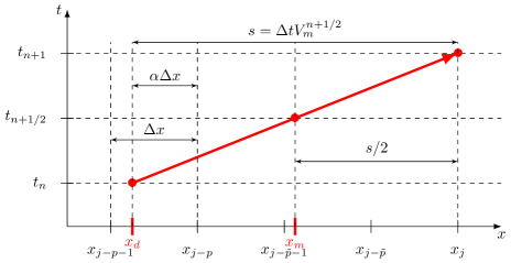
Figure 1: Estimated Lagrangian trajectory in $[t_{n},t_{n+1}]$

Let us first analyze the term accounting for the interpolation error. We consider here a cubic Lagrange interpolation, so we have

(20) $$(\tau_{j}^{n+1})_{2} :=\frac{1}{\Delta t}\left[\varphi_{0}(\Delta tL)u^{n}_{d}-\varphi_{0}(\Delta tL)\sum_{k=-r}^{q}\beta_{k}u^{n}_{j-p+k}\right]=\frac{\varphi_{0}(\Delta tL)}{\Delta t}\left[u^{n}_{d}-\sum_{k=-2}^{1}\beta_{k}u^{n}_{j-p-k}\right]$$

with

(21) $$\begin{gathered}\beta_{-2}=-\frac{\alpha(1-\alpha^{2})}{6},\qquad\beta_{-1}=\frac{\alpha(1+\alpha)(2-\alpha)}{2},\\ \beta_{0}=\frac{(1-\alpha^{2})(2-\alpha)}{2},\qquad\beta_{1}=-\frac{\alpha(1-\alpha)(2-\alpha)}{6}\end{gathered}$$

with $\alpha$ defined such that $x_{j-p}-x_{d}=\alpha\Delta x$ (see Figure 1). Expanding each term in the summation around $u^{n}_{d}$, we get

(22) $$(\tau^{n+1}_{j})_{2} =\frac{\varphi_{0}(\Delta tL)}{\Delta t}\left[u^{n}_{d}-\sum_{k=-2}^{1}{\beta_{k}\left(u^{n}_{d}+\sum_{p=1}^{3}\frac{(k+\alpha)^{p}\Delta x^{p}}{p!}u^{(p)}|^{n}_{d}+\mathcal{O}((k+\alpha)^{4}\Delta x^{4})\right)}\right]$$

$$=\varphi_{0}(\Delta tL)\frac{\Delta x^{3}}{18\Delta t}\alpha(1-\alpha^{2})(2-\alpha)(2\alpha^{2}-2\alpha-1)u_{xxx}|_{d}^{n}+\mathcal{O}\left(\frac{\Delta x^{4}}{\Delta t}\right)=\mathcal{O}\left(\frac{\Delta x^{3}}{\Delta t}\right)$$

and, by considering $\Delta x$ to be kept proportional to $\Delta t$ in a convergence analysis, we have $(\tau_{j}^{n+1})_{2}=\mathcal{O}(\Delta x^{2})=\mathcal{O}(\Delta t^{2})$.

We now develop the truncation error term accounting for the error in the trajectory estimation. Expanding $u^{n+1}_{j}$ around $u_{d}^{n}$ and expanding $\varphi_{0}(\Delta tL)$ around $0$, we have

(23) $$(\tau_{j}^{n+1})_{1}= \frac{1}{\Delta t}\left[u^{n}_{d}+\Delta tu_{t}|_{d}^{n}+su_{x}|_{d}^{n}+\frac{\Delta t^{2}}{2}u_{tt}|_{d}^{n}+\Delta tsu_{tx}|_{d}^{n}+\frac{s^{2}}{2}u_{xx}|_{d}^{n}-\left(1+\Delta tL+\frac{\Delta t^{2}L^{2}}{2}\right)u_{d}^{n}\right]$$

$$+\mathcal{O}(\Delta t^{2})+\mathcal{O}\left(\frac{s^{3}}{\Delta t}\right)$$

where $s:=x_{j}-x_{d}$. The trajectory is estimated considering the velocity field to be constant in $[t_{n},t_{n+1}]$ and equal to its value at the intermediate time step, which is approximated using linear interpolation and extrapolation (see Eq. (12)):

(24) $$s =x_{j}-x_{d}=\frac{\Delta t}{2}\left[2v(t_{n},x_{d})-v(t_{n-1},x_{d})+v(t_{n},x_{j})\right]$$

$$=\frac{\Delta t}{2}\left[2v_{d}^{n}-(v_{d}^{n}-\Delta tv_{t}|_{d}^{n}+\mathcal{O}(\Delta t^{2}))+(v_{d}^{n}+sv_{x}|_{d}^{n}+\mathcal{O}(s^{2}))\right]$$

$$=\Delta tv_{d}^{n}+\frac{\Delta t^{2}}{2}v_{t}|_{d}^{n}+\frac{\Delta ts}{2}v_{x}|_{d}^{n}+\mathcal{O}(\Delta t^{3})+\mathcal{O}(\Delta ts^{2})$$

Replacing $s$ into itself, we get

(25) $$s=\Delta tv_{d}^{n}+\frac{\Delta t^{2}}{2}\left(v_{t}|_{d}^{n}+v_{d}^{n}v_{x}|_{d}^{n}\right)+\mathcal{O}(\Delta t^{3})=\Delta tv_{d}^{n}+\frac{\Delta t^{2}}{2}Lv|_{d}^{n}+\mathcal{O}(\Delta t^{3})$$

Therefore,

(26) $$(\tau^{n+1}_{j})_{1} =\frac{1}{\Delta t} \left[u_{d}^{n}+\Delta tu_{t}|_{d}^{n}+\left(\Delta tv_{n}^{d}+\frac{\Delta t^{2}}{2}Lv|_{d}^{n}+\mathcal{O}(\Delta t^{3})\right)u_{x}|_{d}^{n}+\frac{\Delta t^{2}}{2}u_{tt}|_{d}^{n}\right.$$

$$\left.+\Delta t\left(\Delta tv_{n}^{d}+\frac{\Delta t^{2}}{2}Lv|_{d}^{n}+\mathcal{O}(\Delta t^{3})\right)u_{tx}|_{d}^{n}\right.$$

$$\left.+\frac{1}{2}\left(\Delta tv_{n}^{d}+\frac{\Delta t^{2}}{2}Lv|_{d}^{n}+\mathcal{O}(\Delta t^{3})\right)^{2}u_{xx}|_{d}^{n}\right.$$

$$\left.-\left(1+\Delta tL+\frac{\Delta t^{2}L^{2}}{2}\right)u_{d}^{n}\right]+\mathcal{O}(\Delta t^{2})+\mathcal{O}\left(\frac{\Delta x^{3}}{\Delta t}\right)$$

$$=\frac{1}{\Delta t} \left[\Delta tLu_{d}^{n}+\frac{\Delta t^{2}}{2}L^{2}u_{d}^{n}+\frac{\Delta t^{2}}{2}(Lv_{d}^{n})u_{x}|_{d}^{n}-\left(\Delta tL+\frac{\Delta t^{2}L^{2}}{2}\right)u_{d}^{n}\right.$$

$$\left.+\mathcal{O}(\Delta t^{3})+\mathcal{O}\left(\frac{s^{3}}{\Delta t}\right)\right]$$

$$=\frac{\Delta t}{2} (Lv_{d}^{n})u_{x}|_{d}^{n}+\mathcal{O}(\Delta t^{2})$$

i.e., the scheme (16) provides a first-order approximation to (17). This result shows that the proposed discretization of the linear term (Eq. (14a)) is not able to cancel all out second-order terms, which motivates us to formulate a new discretization in the next section. Also note that, in the case of a constant velocity field, the SE12 scheme provides second-order accuracy, since $Lv_{d}^{n}=v_{t}|_{d}^{n}+(vv_{x})|_{d}^{n}=0$.

5 Second-order semi-Lagrangian exponential integration method

The truncation error analysis presented above indicates that the approximation of the linear term is responsible for the first-order accuracy of the SE12 scheme. Therefore, we provide an alternative formulation for this approximation which is effectively a second-order one:

(27a) $$\boldsymbol{U}^{n+1}_{\text{SE21}} =\varphi_{0}\left(\frac{\Delta tL}{2}\right)\left[\varphi_{0}\left(\frac{\Delta tL}{2}\right)\boldsymbol{U}^{n}\right]^{n}_{*}+\varphi_{0}(\Delta tL)\left[\Delta t\psi_{1}(\Delta tL)\tilde{\boldsymbol{N}}(\boldsymbol{U}^{n})\right]_{*}^{n},$$

(27b) $$\boldsymbol{U}^{n+1}_{\text{SE22}} =\boldsymbol{U}^{n+1}_{\text{SE21}}+\Delta t\varphi_{0}(\Delta tL)\left[\psi_{2}(\Delta tL)\tilde{\boldsymbol{N}}(\boldsymbol{U}^{n+1}_{\text{SE21}})-\left(\psi_{2}(\Delta tL)\tilde{\boldsymbol{N}}(\boldsymbol{U}^{n})\right)^{n}_{*}\right].$$

The names of the methods were chosen following the same reasoning as before. In (27a), a second- and first-order discretizations of the linear and nonlinear terms, respectively, result in a global first-order approximation; in (27b), a global second-order accuracy is ensured by second-order discretizations of both linear and nonlinear terms.

In the following paragraphs, we prove analytically the second-order convergence considering only the linear term. In order to provide a more complete comparative study with the original formulation of the SL-ETDRK schemes, as well as with SL-SI-SETTLS and the Eulerian ETDRK methods, we also present an estimate of the computing complexity and, in Section 6, a detailed linear stability analysis. In Section 7, we provide a numerical verification of these aspects considering the full nonlinear SWE on the rotating sphere.

It is worth noting that linear and interpolation operators do no commute in general (see Appendix of [24]), such that, even with $\varphi_{0}(\Delta tL/2)\varphi_{0}(\Delta tL/2)=\varphi_{0}(\Delta tL)$, we may have

(28) $$\varphi_{0}(\Delta tL)[\boldsymbol{U}^{n}]^{n}_{*}\neq\varphi_{0}\left(\frac{\Delta tL}{2}\right)\left[\varphi_{0}\left(\frac{\Delta tL}{2}\right)\boldsymbol{U}^{n}\right]^{n}_{*}.$$

Finally, we highlight the similarities and differences of the proposed method w.r.t. the semi-Lagrangian Rosenbrock-type exponential schemes proposed by [33]. In both methods, a splitting of the time step integration is performed in order to achieve second-order accuracy. In [33], this is made by evolving the fluid particles along the Lagrangian trajectory from $t_{n}$ to $t_{n+1/2}:=t_{n}+\Delta t/2$, applying the exponential operator at $t_{n+1/2}$, and evolving the fluid particles from $t_{n+1/2}$ to $t_{n}$. Here, we consider a different splitting, with two applications of the exponential operator and a single application of the semi-Lagrangian approach; also, both applications of the exponential operator are identical, corresponding to a left multiplication by the constant matrix $\varphi_{0}(\Delta tL/2)$. Moreover, as described in Section 3.1, we consider a spectral discretization in space, which, with a proper rearrangement of the terms of the governing equations, allows for a straightforward computation of the matrix exponentials, while these are approximated in [33] using Krylov-subspace methods.

5.1 Truncation error analysis

We conduct a similar reasoning as before to compute the truncation error of the scheme

(29) $$U^{n+1}=\varphi_{0}\left(\frac{\Delta tL}{2}\right)\left[\varphi_{0}\left(\frac{\Delta tL}{2}\right)U^{n}\right]^{n}_{*}$$

approximating Eq. (17). Three steps can be identified in this approximation: (i) evolution along the trajectory from $(t_{n},x_{d})$ to the midpoint $(t_{n+1/2},x_{m})$; (ii) interpolation of the computed solution to the midpoint; (iii) evolution along the trajectory from $(t_{n+1/2},x_{m})$ to $(t_{n+1},x_{j})$. Therefore, the truncation error can be written as

(30) $$\tau_{j}^{n+1} = \frac{1}{\Delta t}\left[u^{n+1}_{j}-\varphi_{0}\left(\frac{\Delta tL}{2}\right)\sum_{k=-r}^{q}\beta_{k}\varphi_{0}\left(\frac{\Delta tL}{2}\right)u^{n}_{j-p+k}\right]$$

$$= \underbrace{\frac{1}{\Delta t}\left[u^{n+1}_{j}-\varphi_{0}\left(\frac{\Delta tL}{2}\right)u^{n+1/2}_{m}\right]}_{(\tau_{j}^{n+1})_{1}}+$$

$$\underbrace{\frac{1}{\Delta t}\left[\varphi_{0}\left(\frac{\Delta tL}{2}\right)u^{n+1/2}_{m}-\varphi_{0}\left(\frac{\Delta tL}{2}\right)\sum_{k=-r}^{q}\beta_{k}u^{n+1/2}_{j-\tilde{p}+k}\right]}_{(\tau_{j}^{n+1})_{2}}+$$

$$\underbrace{\frac{1}{\Delta t}\left[\varphi_{0}\left(\frac{\Delta tL}{2}\right)\sum_{k=-r}^{q}\beta_{k}u^{n+1/2}_{j-\tilde{p}+k}-\varphi_{0}\left(\frac{\Delta tL}{2}\right)\sum_{k=-r}^{q}\beta_{k}\varphi_{0}\left(\frac{\Delta tL}{2}\right)u^{n}_{j-p+k}\right]}_{(\tau_{j}^{n+1})_{3}}$$

where $j-\tilde{p}$ is the index of the closest grid point to the right of $x_{m}$ (see Figure 1). Since the trajectory is considered to be linear in the SETTLS approximation, $x_{m}$ satisfies $x_{j}-x_{m}=s/2=\Delta tV^{n+1/2}_{m}/2$.

The first term in (30) ($(\tau^{n+1}_{j})_{1}$) accounts for the error on the estimation of the point $x_{m}$; the second term ($(\tau^{n+1}_{j})_{2}$) accounts for the interpolation error, and the last term ($(\tau^{n+1}_{j})_{3}$) accounts for the error on the estimation of $x_{d}$. The second term is completely analogous to (22), so it is $\mathcal{O}(\Delta x^{3}/\Delta t)$.

The first term in (30) reads

(31) $$(\tau_{j}^{n+1})_{1} =\frac{1}{\Delta t} \left[u^{n+1}_{j}-\varphi_{0}\left(\frac{\Delta tL}{2}\right)u_{m}^{n+1/2}\right]$$

$$=\frac{1}{\Delta t} \left[u^{n+1/2}_{m}+\frac{\Delta t}{2}u_{t}|_{m}^{n+1/2}+\frac{s}{2}u_{x}|_{m}^{n+1/2}+\right.$$

$$+\frac{\Delta t^{2}}{8}u_{tt}|_{m}^{n+1/2}+\frac{\Delta ts}{4}u_{tx}|_{m}^{n+1/2}+\frac{s^{2}}{8}u_{xx}|_{m}^{n+1/2}+\mathcal{O}(\Delta t^{3})+\mathcal{O}(s^{3})$$

$$\left.-\left(1+\frac{\Delta tL}{2}+\frac{\Delta t^{2}L^{2}}{8}+\mathcal{O}(\Delta t^{3})\right)u_{m}^{n+1/2}\right]$$

$$=\frac{1}{\Delta t} \left[\frac{\Delta t}{2}\left(u_{t}|_{m}^{n+1/2}+vu_{x}|_{m}^{n+1/2}-Lu_{m}^{n+1/2}\right)\right.$$

$$\left.+\frac{\Delta t^{2}}{8}\left(u_{tt}|_{m}^{n+1/2}+2(vu)|_{m}^{n+1/2}+(v^{2}u_{xx})|_{m}^{n+1/2}-L^{2}u_{m}^{n+1/2}\right)+\mathcal{O}(\Delta t^{3})\right]$$

$$=\frac{1}{\Delta t} \left[\frac{\Delta t^{2}}{8}\left(u_{tt}|_{m}^{n+1/2}+2(vu)|_{m}^{n+1/2}+(v^{2}u_{xx})|_{m}^{n+1/2}-L^{2}u_{m}^{n+1/2}\right)+\mathcal{O}(\Delta t^{3})\right]$$

where we used the facts that $Lu=u_{t}+vu_{x}$ and

(32) $$s=x_{j}-x_{d}=\frac{\Delta t}{2}\left(2v(t_{n},x_{d})-v(t_{n-1},x_{d})+v(t_{n},x_{j})\right)=\Delta tv_{m}^{n+1/2}+\mathcal{O}(\Delta t^{3})$$

For computing the last term in (30), we note that, from (22), the cubic interpolation yields

(33) $$\sum_{k=-r}^{q}{\beta_{k}w_{j-p+k}}=w_{d}+\mathcal{O}(\Delta x^{3}),\qquad\sum_{k=-r}^{q}{\beta_{k}w_{j-\tilde{p}+k}}=w_{m}+\mathcal{O}(\Delta x^{3})$$

for any function $w=w(x)$. Therefore,

(34) $$\left(\tau_{j}^{n+1}\right)_{3} =\frac{1}{\Delta t} \left[\varphi_{0}\left(\frac{\Delta tL}{2}\right)\sum_{k=-r}^{q}\beta_{k}u^{n+1/2}_{j-\tilde{p}+k}-\varphi_{0}\left(\frac{\Delta tL}{2}\right)\sum_{k=-r}^{q}\beta_{k}\varphi_{0}\left(\frac{\Delta tL}{2}\right)u^{n}_{j-p+k}\right]$$

$$=\frac{1}{\Delta t} \varphi_{0}\left(\frac{\Delta tL}{2}\right)\left[u^{n+1/2}_{m}-\varphi_{0}\left(\frac{\Delta tL}{2}\right)u^{n}_{d}+\mathcal{O}(\Delta x^{3})\right]$$

$$=\frac{1}{\Delta t} \left(1+\frac{\Delta tL}{2}+\frac{\Delta t^{2}L^{2}}{8}+\mathcal{O}(\Delta t^{3})\right)\left[u^{n+1/2}_{m}-\left(1+\frac{\Delta tL}{2}+\frac{\Delta t^{2}L^{2}}{8}+\mathcal{O}(\Delta t^{3})\right)\right.$$

$$\left.\left(u^{n+1/2}_{m}-\frac{\Delta t}{2}u_{t}|_{m}^{n+1/2}-\frac{s}{2}u_{x}|_{m}^{n+1/2}\right.\right.$$

$$\left.\left.+\frac{\Delta t^{2}}{8}u_{tt}|_{d}^{n+1/2}+\frac{\Delta ts}{4}u_{tx}|_{d}^{n+1/2}+\frac{s^{2}}{8}u_{xx}|_{d}^{n+1/2}+\mathcal{O}(\Delta t^{3})\right)+\mathcal{O}(\Delta x^{3})\right]$$

$$=\frac{1}{\Delta t} \left[\frac{\Delta t}{2}\left(-Lu_{m}^{n+1/2}+u_{t}|_{m}^{n+1/2}+(vu_{x})|_{m}^{n+1/2}\right)\right.$$

$$\left.+\frac{\Delta t^{2}}{8}\left(-3L^{2}u_{m}^{n+1/2}+4Lu_{t}|_{m}^{n+1/2}+2L(vu_{x})|_{m}^{n+1/2}\right.\right.$$

$$\left.\left.-u_{tt}|_{m}^{n+1/2}-2(vu_{tx})|_{m}^{n+1/2}-(v^{2}u_{xx})|_{m}^{n+1/2}\right)+\mathcal{O}(\Delta t^{3})+\mathcal{O}(\Delta x^{3})\right]$$

$$=\frac{1}{\Delta t} \left[\frac{\Delta t^{2}}{8}\left(-3L^{2}u_{m}^{n+1/2}+4Lu_{t}|_{m}^{n+1/2}+2L(vu_{x})|_{m}^{n+1/2}\right.\right.$$

$$\left.\left.-u_{tt}|_{m}^{n+1/2}-2(vu_{tx})|_{m}^{n+1/2}-(v^{2}u_{xx})|_{m}^{n+1/2}\right)\right.$$

$$\left.+\mathcal{O}(\Delta t^{3})+\mathcal{O}(\Delta x^{3})\right]$$

Adding the three terms in (30), we get

(35) $$\tau_{j}^{n+1} =\frac{1}{\Delta t}\left[\frac{4\Delta t^{2}L}{8}\left(-Lu_{m}^{n+1/2}+u_{t}|_{m}^{n+1/2}+(vu_{x})|_{m}^{n+1/2}\right)\right]+\mathcal{O}(\Delta t^{2})+\mathcal{O}\left(\frac{\Delta x^{3}}{\Delta t}\right)$$

$$=\mathcal{O}(\Delta t^{2})$$

thus yielding a second-order approximation.

5.2 Computational complexity

We now provide an estimate of the computational complexity of the proposed modified semi-Lagrangian exponential methods and the other time integration schemes considered here. In each time step, the following computations are performed:

• In the case of exponential methods, the evaluation of the $\varphi_{k}$ and/or the $\psi_{k}$ functions. Since these functions are defined recursively, their cost increases for larger $k$. These functions need to be computed for each pair of wavenumber $(m,n)$, and we recall that the matrix exponentials are computed in this work considering the diagonalization of the matrix (eq. (10)), such that we need only to compute the exponential of the eigenvalues of $\boldsymbol{L}=\boldsymbol{L}_{\boldsymbol{G}}$ (two per wavenumber pair);

• In the case of semi-Lagrangian schemes, the trajectories need to be estimated, and spatial interpolations to the departure points need to be performed;

• In the case of SL-SI-SETTLS (13), the semi-implicit discretization for the linear term requires both the application of $\boldsymbol{L}$ and $\boldsymbol{L}^{-1}$, the latter through the solution of a Helmholtz equation [36];

• Finally, all schemes require the evaluation of at least one nonlinear term.

Table 1 summarizes the number of each operation listed above performed by each time integration scheme. In this table, each $\varphi_{k}/\psi_{k}$ function is depicted individually; $\boldsymbol{x}_{d}$ and $()_{*}$ denote respectively the evaluation of the Lagrangian trajectories and the interpolation to the departure points; $\boldsymbol{L}$ and $\boldsymbol{L}^{-1}$ correspond to the semi-implicit scheme described above; and $\boldsymbol{N}_{\boldsymbol{A}}$ and $\boldsymbol{N}_{\boldsymbol{R}}$ indicate the evaluation of the (respectively advection and remaining) nonlinear terms.

Scheme	$\varphi_{0}$	$\varphi_{1}$	$\varphi_{2}$	$\psi_{1}$	$\psi_{2}$	$\boldsymbol{x}_{d}$	$()_{*}$	$L$	$L^{-1}$	$\boldsymbol{N}_{\boldsymbol{A}}$	$\boldsymbol{N}_{\boldsymbol{R}}$
ETD1RK	1	1	0	0	0	0	0	0	0	1	1
ETD2RK	1	1	1	0	0	0	0	0	0	2	2
SE11	1	0	0	1	0	1	1	0	0	0	1
SE12	2	0	0	1	2	1	2	0	0	0	2
SE21	3	0	0	1	0	1	2	0	0	0	1
SE22	4	0	0	1	2	1	3	0	0	0	2
SL-SI-SETTLS	0	0	0	0	0	1	2	1	1	0	2

Table 1: Number of operations performed per time step by each time integration scheme. $\boldsymbol{x}_{d}$ and $()_{*}$ denote respectively the evaluation of the Lagrangian trajectories and the interpolation to the departure points; $\boldsymbol{L}$ and $\boldsymbol{L}^{-1}$ correspond to the semi-implicit scheme.

It is clear from this table that the proposed modifications of the semi-Lagrangian exponential schemes introduce additional complexity per time step, with two more exponential evaluations and one more spatial interpolation w.r.t. their respective original formulations. However, as assessed in the numerical simulations presented in Section 7, the improved accuracy and stability of SE22 allow us to choose larger time step sizes. Moreover, it has been identified in the numerical simulations that the computation of the exponential functions is responsible for an important fraction of the computing time in our implementation, such that important savings are possible by precomputing them; additional savings could also be obtained with a more efficient implementation (e.g., by using vectorization).

6 Linear stability analysis

In the following paragraphs, we conduct a stability study comparing exponential and semi-Lagrangian exponential schemes, as well as SL-SI-SETTLS. Linear stability analyses of Eulerian exponential schemes have been conducted, e.g., by [7, 8, 3]. The last two cited works show notably that these methods are in general unstable when applied to non-diffusive problems, but depending on configurations of the problem and the exponential scheme, the amplifications are small such that instabilities may remain unnoticed within the simulation time. In this section, we focus on comparing stability regions of both Eulerian and semi-Lagrangian schemes.

The stability study proposed here is inspired by the procedure presented by [7]. Consider a generic nonlinear ODE in the form

(36) $$\dot{u}=\lambda_{\boldsymbol{L}}u+\boldsymbol{N}(u)$$

Substituting $u=\overline{u}+u^{\prime}$ in (36), where $\overline{u}$ is a steady state (i.e., $\lambda_{\boldsymbol{L}}\overline{u}+\boldsymbol{N}(\overline{u})=0$) and $u^{\prime}$ is a perturbation, expanding $N(\overline{u}+u^{\prime})$ around $\overline{u}$, truncating at first order and defining $\lambda_{\boldsymbol{N}}:=\boldsymbol{N}^{\prime}(\overline{u})$, we obtain the linearized equation

(37) $$\dot{u}^{\prime}=\lambda_{\boldsymbol{L}}u^{\prime}+\lambda_{\boldsymbol{N}}u^{\prime}$$

which we consider hereafter, with the primes omitted for conciseness. However, we need to take into account that we are comparing both Eulerian (ETDRK) and semi-Lagrangian (SL-SI-SETTLS and SE**) methods, and this study should be able to capture the influence of advective effects and interpolation procedures. In the case of SL schemes, the advection is incorporated into the material derivative, and we can directly use the same linearized ODE as above:

(38) $$\frac{du}{dt}=\lambda_{\boldsymbol{L}}u+\lambda_{\boldsymbol{N}}u$$

where $u,\lambda_{\boldsymbol{L}},\lambda_{\boldsymbol{N}}\in\mathbb{C}$. This equation arises, e.g., when (5) is solved using a spectral method, in which case $u=\hat{u}_{k}(t)$ is a spectral coefficient of the solution, and $\lambda_{\boldsymbol{L}}$, $\lambda_{\boldsymbol{N}}$ are modes associated respectively to $\boldsymbol{L}$ and the linearized term $\boldsymbol{N}$. If $\boldsymbol{L}$ and $\boldsymbol{N}$ are diagonalizable in the spectral space with the same set of eigenvectors, then (5) leads to a system of uncoupled ODEs of the form (38), each one corresponding to a wavenumber $k$.

On the other hand, in the case of Eulerian schemes, we need to consider the advection explicitly, leading to a linearized one-dimensional scalar advection equation with source term:

(39) $$\frac{\partial u}{\partial t}+v\frac{\partial u}{\partial x}=\lambda_{\boldsymbol{L}}u+\boldsymbol{N}(u)\implies\frac{\partial u}{\partial t}+v\frac{\partial u}{\partial x}=\lambda_{\boldsymbol{L}}u+\lambda_{\boldsymbol{N}}u$$

in which the spatial derivative becomes a scalar multiplication when solved in the spectral space, and $v$ is a scalar velocity field assumed to be constant for simplicity.

The stability region of a given numerical scheme with stability function $A:=|u^{n+1}/u^{n}|$ is defined as the region in $\mathbb{C}^{2}$ in which $|A(\Delta t\lambda_{\boldsymbol{L}},\Delta t\lambda_{\boldsymbol{N}})|\leq 1$, where $u^{n}=u(t_{n},x)=A^{n}e^{i\kappa x}$ is the computed approximation to $u(t_{n})$, $\kappa=2\pi k/L$ is the normalized wavenumber and $L$ is the length of the spatial domain. A complete stability study should be performed in a four-dimensional space, since $A$ depends on the real and imaginary parts of $\lambda_{\boldsymbol{L}}$ and $\lambda_{\boldsymbol{N}}$; however, since a hyperbolic problem such as the SWE propagates purely hyperbolic modes, we simplify this study by fixing values of $\xi_{\boldsymbol{L}}:=\Delta t\lambda_{\boldsymbol{L}}\in i\mathbb{R}$ (since the eigenvalues of $\boldsymbol{L}$ are purely imaginary) and plotting the amplification factors as functions of $Im(\xi_{\boldsymbol{N}})$, where $\xi_{\boldsymbol{N}}:=\Delta t\lambda_{\boldsymbol{N}}$.

6.1 Stability of ETD1RK and ETD2RK

When applying (7a) and (7b) to (39), the advection term could be treated either as a linear or nonlinear term, yielding different stability functions. We consider only the latter case, but the overall conclusions on the stability of ETD1RK and ETD2RK compared to the other schemes considered in this work are similar. We have

(40a) $$u^{n+1}_{\text{ETD1RK}} =\varphi_{0}(\xi_{\boldsymbol{L}})u^{n}+\Delta t\varphi_{1}(\xi_{\boldsymbol{L}})\lambda_{\boldsymbol{N}}u^{n}-\Delta t\varphi_{1}(\xi_{\boldsymbol{L}})iv\kappa u^{n}$$

$$=\left[\varphi_{0}(\xi_{\boldsymbol{L}})+\varphi_{1}(\xi_{\boldsymbol{L}})(\xi_{\boldsymbol{N}}-i\kappa s)\right]u^{n}$$

(40b) $$u^{n+1}_{\text{EDT2RK}} =u^{n+1}_{\text{ETD1RK}}+\Delta t\varphi_{2}(\xi_{\boldsymbol{L}})\left[(\lambda_{\boldsymbol{N}}-iv\kappa)u^{n+1}_{\text{ETD1RK}}-(\lambda_{\boldsymbol{N}}-vi\kappa)u^{n}\right]$$

$$=u^{n+1}_{\text{ETD1RK}}+\varphi_{2}(\xi_{\boldsymbol{L}})\left(\xi_{\boldsymbol{N}}-i\kappa s\right)\left(u^{n+1}_{\text{ETD1RK}}-u^{n}\right)$$

where $s:=v\Delta t=x_{j}-x_{*}$ is the spatial displacement of each particle from $t_{n}$ to $t_{n+1}$ (see Figure 1). Note that we have considered the spatial derivative to be computed exactly (which can be achieved, e.g., by using a spectral method, as considered in this work), i.e., $(u^{n})_{x}=i\kappa u^{n}$, since we want to analyze exclusively the stability properties due to the temporal discretization.

Thus, the stability functions of the Eulerian ETD1RK and ETD2RK schemes read

(41a) $$A_{\text{ETD1RK}} =\varphi_{0}(\xi_{\boldsymbol{L}})+\varphi_{1}(\xi_{\boldsymbol{L}})(\xi_{\boldsymbol{N}}-i\kappa s)$$

(41b) $$A_{\text{ETD2RK}} =A_{\text{ETD1RK}}+\varphi_{2}(\xi_{\boldsymbol{L}})\left(\xi_{\boldsymbol{N}}-i\kappa s\right)\left[A_{\text{ETD1RK}}-1\right]$$

Note that the presence of the term $-i\kappa s$ makes the stability regions dependent on the spatial information. This implies that the schemes may not be simultaneously stable for a large range of wavenumbers, since the intersection of their stability regions may be small or even empty. Following [16], we compute stability functions $A_{\kappa s}=A_{\kappa s}(\xi_{\boldsymbol{L}},\xi_{\boldsymbol{N}})$ for $\kappa s\in\mathcal{K}:=\{0,\pi/10,2\pi/10,\dots,2\pi\}$; then, for each $(\xi_{\boldsymbol{L}},\xi_{\boldsymbol{N}})$, the amplification factor is $A(\xi_{\boldsymbol{L}},\xi_{\boldsymbol{N}})=\max_{\kappa s\in\mathcal{K}}A_{\kappa s}(\xi_{\boldsymbol{N}},\xi_{\boldsymbol{L}})$.

6.2 Stability of SL-SI-SETTLS

We now develop a linear stability analysis for the semi-implicit semi-Lagrangian SETTLS [16] described in Section 3.2. In the stability analysis of semi-Lagrangian schemes, we also need to take into account the spatial dependence of the solution. Using $u(t_{n},x)=A^{n}e^{i\kappa x}$ in (13) applied to (38), we obtain

(42) $$A^{n+1}e^{i\kappa x_{j}}-A^{n}e^{i\kappa x_{*}}=\frac{\xi_{\boldsymbol{L}}}{2}\left(A^{n+1}e^{i\kappa x_{j}}+A^{n}e^{i\kappa x_{*}}\right)+\frac{\xi_{\boldsymbol{N}}}{2}\left(\left[2A^{n}-A^{n-1}\right]e^{i\kappa x_{*}}+A^{n}e^{i\kappa x_{j}}\right)$$

which, after division by $A^{n-1}e^{i\kappa x_{j}}$ and recalling that $s:=x_{j}-x_{*}$, leads to the quadratic equation

(43) $$A^{2}\left(1-\frac{\xi_{\boldsymbol{L}}}{2}\right)-A\left(e^{-i\kappa s}\left(1+\frac{\xi_{\boldsymbol{L}}}{2}+\xi_{\boldsymbol{N}}\right)+\frac{\xi_{\boldsymbol{N}}}{2}\right)+\frac{\xi_{\boldsymbol{N}}}{2}e^{-i\kappa s}=0$$

whose roots $A=A_{\text{SL-SI-SETTLS}}$ define the stability function of SL-SI-SETTLS; its stability region is the intersection between the stability regions defined by each of the two roots of (43). Moreover, as in the case of ETD1RK and ETD2RK considering the advection term, these roots depend on the spatial wavenumber through the term $e^{-i\kappa s}$, and the stability region is defined as the intersection of the individual stability regions for each $\kappa s$.

6.3 Stability of SE11 and SE12

We now study the stability of the semi-Lagrangian exponential schemes proposed by [24] and described in Section 3.3. Using $u(x,t_{n})=A^{n}e^{i\kappa x}$ in (14a) and (14b) applied to (38) and the fact that $\varphi_{k}(z)=\varphi_{0}(z)\psi_{k}(z)\ \forall k>0$, we get

(44a) $$A_{\text{SE11}} =\varphi_{0}(\xi_{\boldsymbol{L}})e^{-i\kappa s}+\xi_{\boldsymbol{N}}\varphi_{1}(\xi_{\boldsymbol{L}})e^{-i\kappa s}=e^{-i\kappa s}\varphi_{0}(\xi_{\boldsymbol{L}})[1+\xi_{\boldsymbol{N}}\psi_{1}(\xi_{\boldsymbol{L}})]$$

(44b) $$A_{\text{SE12}} =A_{\text{SE11}}+\xi_{\boldsymbol{N}}\varphi_{2}(\xi_{\boldsymbol{L}})\left[A_{\text{SE11}}-e^{-i\kappa s}\right]$$

$$=e^{-i\kappa s}\left[\left(1+\xi_{\boldsymbol{N}}\varphi_{2}(\xi_{\boldsymbol{L}})\right)\varphi_{0}(\xi_{\boldsymbol{L}})\left(1+\xi_{\boldsymbol{N}}\psi_{1}(\xi_{\boldsymbol{L}})\right)-\xi_{\boldsymbol{N}}\varphi_{2}(\xi_{\boldsymbol{L}})\right]$$

Since $|e^{-iks}|=1$, the stability regions of both SE11 and SE12 do not depend on $\kappa s$. This is a remarkable feature of these schemes, since, contrary to what happens to SL-SI-SETTLS, there is no reduction of the global stability region when intersecting the regions corresponding to each wavenumber.

We compare in Figure 2 the stability functions of ETD1RK and ETD2RK applied to (39), and SL-SI-SETTLS, SE11 and SE12 applied to (38). We present the regions for integer multiples of $\tilde{\xi}_{\boldsymbol{L}}=i\sqrt{\overline{\Phi}/a^{2}}\approx 2.5\times 10^{-4}i$, which is obtained from an approximation to the eigenvalues $\lambda_{\boldsymbol{L}}=i\sqrt{\overline{\Phi}n(n+1)/a^{2}}$ of $\boldsymbol{L}=\boldsymbol{L}_{\boldsymbol{G}}$ considering relevant physical parameters and an f-plane approximation (see [4] for details). The scaling of $\tilde{\xi}_{\boldsymbol{L}}$ can be seen as a result of different choices of time step size $\Delta t$ and/or wavenumbers: for instance, the plot considering $\xi_{\boldsymbol{L}}=20000\tilde{\xi}_{\boldsymbol{L}}$ in Figure 2 corresponds to the stability region of the maximum wavenumber in a spectral resolution $M=256$ and a reasonable time step size of approximately $\Delta t=80\text{s}$. The plots reveal notably an enhancement of the stability of the semi-Lagrangian exponential schemes when compared to their Eulerian counterparts, which suffer from a small intersection of the stability regions of each $\kappa s$, indicating that the schemes have a lack of stability common to a large range of combinations between wavenumbers and spatial displacement. The semi-Lagrangian exponential scheme with second-order discretization of the nonlinear term (SE12) also presents a considerably larger stability region compared to SL-SI-SETTLS.

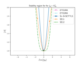
(a) $\xi_{\boldsymbol{L}}=0$

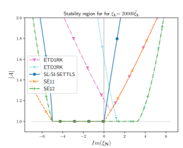
(b) $\xi_{\boldsymbol{L}}=20000\tilde{\xi}_{\boldsymbol{L}}$

Figure 2: Stability functions of ETD1RK and ETD2RK applied to (39) (considering a nonlinear treatment of the advection term), and SL-SI-SETTLS, SE11 and SE12 applied to (38), as a function of $Im(\xi_{\boldsymbol{N}})$ for fixed values of $\xi_{\boldsymbol{L}}$ and $Re(\xi_{\boldsymbol{N}})=0$. The stability regions of ETD1RK and ETD2RK are empty in the case $\xi_{\boldsymbol{L}}=0$. The horizontal, dashed line indicates the boundary of the stability region requiring $|A|\leq 1$.

6.4 Stability of SE21 and SE22

Using the same procedure described above to assess stability properties of the modified schemes SE21 and SE22 (Section 5) does not provide insights on potential stability improvements or decreases induced by the splitting of the matrix exponential. In particular, this approach is not able to capture the fact that the matrix exponential and the interpolation do not commute [24]. Indeed, using $u(x,t_{n})=A^{n}e^{i\kappa x}$ in (27a) and (38), analogously to (44a), provides

(45) $$\varphi_{0}\left(\frac{\xi_{\boldsymbol{L}}}{2}\right)e^{-i\kappa s}\varphi_{0}\left(\frac{\xi_{\boldsymbol{L}}}{2}\right)=e^{\xi_{\boldsymbol{L}}/2}e^{-i\kappa s}e^{\xi_{\boldsymbol{L}}/2}=e^{\xi_{\boldsymbol{L}}}e^{-i\kappa s}=\varphi_{0}(\xi_{\boldsymbol{L}})e^{-i\kappa s}$$

such that $A_{\text{SE21}}\equiv A_{\text{SE11}}$, and, similarly, $A_{\text{SE22}}\equiv A_{\text{SE12}}$. However, different stability properties are verified in the numerical simulations presented in Section 7.

Next, we develop in detail how the differences between the two sets of schemes arise. Consider the ODE (38) with only the linear term:

(46) $$\frac{du}{dt}=\lambda_{\boldsymbol{L}}u$$

We first consider the first-order discretization used in (14a). Since the problem is solved in the spectral space, we may write

(47) $$\hat{u}_{k}^{n+1}=\varphi_{0}({\xi_{\boldsymbol{L}_{k}}})[\hat{u}_{k}^{n}]_{*},\qquad k=-M,\dots,M$$

where $u(t,x)\approx\sum_{k=-M}^{M}\hat{u}_{k}^{n}e^{i\kappa x}$ is the truncated Fourier decomposition of $u$ and $\xi_{\boldsymbol{L}_{k}}:=\Delta t{\lambda_{\boldsymbol{L}_{k}}}$ may depend on $k$. Note, however, that the interpolation is performed on the grid. Therefore, using the direct and inverse discrete Fourier transforms

(48) $$\hat{u}_{k}^{n}=\mathcal{F}(u^{n})=\frac{1}{P}\sum_{j=0}^{P-1}u(t_{n},x_{j})e^{-i\kappa x_{j}},\qquad u(t_{n},x_{j})=\mathcal{F}^{-1}(\hat{u}^{n})=\sum_{k=-M}^{M}\hat{u}^{n}_{k}e^{i\kappa x_{j}}$$

with $\kappa=2\pi k/L$, L the length of the periodic spatial domain and $P+1$ the number of equidistant grid points $x_{i}=i\Delta x$, $i=0,\dots,P$, $\Delta x=L/P$, we may rewrite (47) more rigorously as

(49) $$\hat{u}^{n+1}_{k} =\varphi_{0}(\xi_{\boldsymbol{L}_{k}})\mathcal{F}([\mathcal{F}^{-1}(\hat{u}^{n})]_{*})=\varphi_{0}(\xi_{\boldsymbol{L}_{k}})\mathcal{F}([u^{n}_{j}]_{*})=\varphi_{0}(\xi_{\boldsymbol{L}_{k}})\frac{1}{P}\sum_{j=0}^{P-1}u(t_{n},x_{d_{j}})e^{-i\kappa x_{j}}$$

$$=\varphi_{0}(\xi_{\boldsymbol{L}_{k}})\frac{1}{P}\sum_{j=0}^{P-1}u(t_{n},x_{j-p_{j}})e^{-i\kappa x_{j}}=\varphi_{0}(\xi_{\boldsymbol{L}_{k}})\frac{1}{P}\sum_{j=0}^{P-1}u(t_{n},x_{r_{j}})e^{-i\kappa x_{p_{j}+r_{j}}}$$

$$=\varphi_{0}(\xi_{\boldsymbol{L}_{k}})\frac{1}{P}\sum_{j=0}^{P-1}u(t_{n},x_{r_{j}})e^{-i\kappa(p_{j}+r_{j})\Delta x}$$

where $x_{d_{j}}$ is the departure point at $t_{n}$ of the Lagrangian trajectory arriving at $x_{j}$ at $t_{n+1}$, and, for simplification, $x_{d_{j}}=x_{j-p_{j}}$, $p_{j}\in\mathbb{Z}$, is supposed to belong to the grid (otherwise $u(t_{n},x_{d_{j}})$ may be written as a linear combination (i.e., interpolation) of the solution computed at grid points). If the velocity field is constant in space, then $\forall j,p_{j}=p,r_{j}=r$, thus

(50) $$\hat{u}^{n+1}_{k}=\varphi_{0}(\xi_{\boldsymbol{L}_{k}})e^{-i\kappa p\Delta x}\frac{1}{P}\sum_{r=0}^{P-1}u(t_{n},x_{r})e^{-i\kappa x_{r}}=\varphi_{0}(\xi_{\boldsymbol{L}_{k}})\hat{u}^{n}_{k}e^{-i\kappa p\Delta x}=\varphi_{0}(\xi_{\boldsymbol{L}_{k}})\hat{u}^{n}_{k}e^{-i\kappa s}$$

with $s:=x_{j}-x_{d_{j}}=x_{j}-x_{j-p}=p\Delta x$. Therefore, for each $k$, the stability function $|\hat{u}^{n+1}_{k}|/|\hat{u}^{n}_{k}|=\varphi_{0}(\xi_{\boldsymbol{L}_{k}})e^{-i\kappa s}$ is the same as derived above (see Eq. (44a)). However, if the velocity field is not constant, we are not able to factor out $e^{-i\kappa p_{j}\Delta x}$ from the summation, and the stability function may be different.

Consider now the proposed modification to the discretization of the linear term. In the spectral space, we solve

(51) $$\hat{u}_{k}^{n+1}=\varphi_{0}\left(\frac{\xi_{\boldsymbol{L}_{k}}}{2}\right)\mathcal{F}([\mathcal{F}^{-1}(\hat{w})^{n}]_{*}),\qquad k=-M,\dots,M$$

where

(52) $$\hat{w}^{n}_{k}:=\varphi_{0}\left(\frac{\xi_{\boldsymbol{L}_{k}}}{2}\right)\hat{u}^{n}_{k}$$

Conducting the same development as above,

(53) $$\hat{u}_{k}^{n+1}=\varphi_{0}\left(\frac{\xi_{\boldsymbol{L}_{k}}}{2}\right)\frac{1}{P}\sum_{j=0}^{P-1}w(t_{n},x_{r_{j}})e^{-i\kappa(p_{j}+r_{j})\Delta x}=\varphi_{0}\left(\frac{\xi_{\boldsymbol{L}_{k}}}{2}\right)\hat{w}^{n}_{k}e^{-i\kappa s}=\varphi_{0}(\xi_{\boldsymbol{L}_{k}})\hat{u}^{n}_{k}e^{-i\kappa s}$$

where the second equality holds if the velocity field is constant. We conclude that, if $v$ is constant, the original and the proposed discretizations of the linear term yield the same stability function. However, if the velocity field is not constant, we have

(54) $$\hat{u}_{k}^{n+1} =\varphi_{0}\left(\frac{{\xi_{\boldsymbol{L}_{k}}}}{2}\right)\frac{1}{P}\sum_{j=0}^{P-1}w(t_{n},x_{r_{j}})e^{-i\kappa(p_{j}+r_{j})\Delta x}$$

$$=\varphi_{0}\left(\frac{{\xi_{\boldsymbol{L}_{k}}}}{2}\right)\frac{1}{P}\sum_{j=0}^{P-1}\left[\sum_{l=-M}^{M}\hat{w}^{n}_{l}e^{i\kappa_{l}x_{j}}\right]e^{-i\kappa(p_{j}+r_{j})\Delta x}$$

$$=\varphi_{0}\left(\frac{{\xi_{\boldsymbol{L}_{k}}}}{2}\right)\frac{1}{P}\sum_{j=0}^{P-1}\left[\sum_{l=-M}^{M}\varphi_{0}\left(\frac{{\xi_{\boldsymbol{L}_{l}}}}{2}\right)\hat{u}^{n}_{l}e^{i\kappa_{l}x_{j}}\right]e^{-i\kappa(p_{j}+r_{j})\Delta x}$$

$$\neq\varphi_{0}({\xi_{\boldsymbol{L}_{k}}})\frac{1}{P}\sum_{j=0}^{P-1}u(t_{n},x_{r_{j}})e^{-i\kappa(p_{j}+r_{j})\Delta x}$$

where $\kappa_{l}:=2\pi l/L$. Note that the dependency of ${\xi_{\boldsymbol{L}_{l}}}$ on $l$ prevents us from factoring out the exponential term from the inner summation, such that the inverse Fourier transform into the brackets does not yield $u(t_{n},x_{r_{j}})$. As a consequence, different stability functions are provided by the two variants of the semi-Lagrangian exponential scheme.

Therefore, by explicitly writing the spectral transforms involved in the integration of the semi-Lagrangian exponential schemes, it becomes clear why different discretizations of the linear term lead to different stability functions. We remark, however, that these differences are not necessarily linked to the fact that the equations are solved using a spectral method, but rather to the lack of commutation between the matrix exponential and the interpolation. For illustration, consider the equation

(55) $$\frac{d\boldsymbol{u}}{dt}=\lambda_{\boldsymbol{L}}\boldsymbol{u}$$

defined on the (periodic) physical space, with $\boldsymbol{u}=\left(u_{1},\ \dots,\ u_{P}\right)^{T}\in\mathbb{R}^{P}$ and $\lambda_{\boldsymbol{L}}=\text{diag}(\lambda_{1},\dots,\lambda_{P})\in\mathbb{R}^{P\times P}$ a diagonal matrix with at least one element $\lambda_{i}$ different from the others. Consider also that the interpolation procedure consists simply of a one grid point shift to the right. Therefore, the integration of one time step of (55) using the two variants of the semi-Lagrangian exponential scheme yields respectively

(56) $$\boldsymbol{u}^{n+1}=\varphi_{0}(\Delta t\lambda_{\boldsymbol{L}})[\boldsymbol{u}^{n}]_{*}=\left(\begin{array}[]{c c c}\varphi_{0}(\Delta t\lambda_{1})&&0\\ &\ddots&\\ 0&&\varphi_{0}(\Delta t\lambda_{P})\end{array}\right)\left(\begin{array}[]{c}u^{n}_{P}\\ u^{n}_{1}\\ \vdots\\ u^{n}_{P-1}\end{array}\right)=\left(\begin{array}[]{c}\varphi_{0}(\Delta t\lambda_{1})u^{n}_{P}\\ \varphi_{0}(\Delta t\lambda_{2})u^{n}_{1}\\ \vdots\\ \varphi_{0}(\Delta t\lambda_{P})u^{n}_{P-1}\end{array}\right)$$

and

(57) $$\boldsymbol{u}^{n+1} =\varphi_{0}\left(\frac{\Delta t\lambda_{\boldsymbol{L}}}{2}\right)\left[\varphi_{0}\left(\frac{\Delta t\lambda_{\boldsymbol{L}}}{2}\right)\boldsymbol{u}^{n}\right]_{*}$$

$$=\left(\begin{array}[]{c c c}\varphi_{0}(\Delta t\lambda_{1}/2)&&0\\ &\ddots&\\ 0&&\varphi_{0}(\Delta t\lambda_{P}/2)\end{array}\right)\left[\left(\begin{array}[]{c}\varphi_{0}(\Delta t\lambda_{1}/2)u^{n}_{1}\\ \varphi_{0}(\Delta t\lambda_{2}/2)u^{n}_{2}\\ \vdots\\ \varphi_{0}(\Delta t\lambda_{P}/2)u^{n}_{P}\end{array}\right)\right]_{*}$$

$$=\left(\begin{array}[]{c c c}\varphi_{0}(\Delta t\lambda_{1}/2)&&0\\ &\ddots&\\ 0&&\varphi_{0}(\Delta t\lambda_{P}/2)\end{array}\right)\left[\left(\begin{array}[]{c}\varphi_{0}(\Delta t\lambda_{P}/2)u^{n}_{P}\\ \varphi_{0}(\Delta t\lambda_{1}/2)u^{n}_{1}\\ \vdots\\ \varphi_{0}(\Delta t\lambda_{P-1}/2)u^{n}_{P-1}\end{array}\right)\right]_{*}$$

$$=\left(\begin{array}[]{c}\varphi_{0}(\Delta t\lambda_{1}/2)\varphi_{0}(\Delta t\lambda_{P}/2)u^{n}_{P}\\ \varphi_{0}(\Delta t\lambda_{2}/2)\varphi_{0}(\Delta t\lambda_{1}/2)u^{n}_{1}\\ \vdots\\ \varphi_{0}(\Delta t\lambda_{P}/2)\varphi_{0}(\Delta t\lambda_{P-1}/2))u^{n}_{P-1}\end{array}\right)$$

with the two schemes being equivalent only if $\lambda_{\boldsymbol{L}}$ is a multiple of the identity matrix.

Note that, except for the case in which the velocity field is constant, determining the stability regions of SE** analytically, using (49) and (54), is not feasible. In particular, we are not able to obtain an expression in the form $\hat{u}^{n+1}_{k}=A(\xi_{\boldsymbol{L}},\xi_{\boldsymbol{N}})\hat{u}^{n}_{k}$ for each $k$ separately, and $\hat{u}^{n+1}_{k}$ depends a priori on all wavenumber modes. It means that we are no longer in the framework of a linear stability analysis, even if the problem (38) itself is linear, with this nonlinearity being a consequence of the lack of commutation between the exponential and interpolation operators. We choose therefore to assess the stability properties of the schemes through numerical simulation, as presented in Section 7.2.

7 Numerical tests

In this section, we perform a set of numerical simulations of the SWE on the rotating sphere to evaluate the proposed modifications of the semi-Lagrangian exponential methods and to compare them with their original versions and with other relevant numerical schemes in this study, namely SL-SI-SETTLS and the Eulerian exponential integration methods. We begin by verifying the numerical orders of convergence using benchmark test cases with increasing complexity; then, we conduct an empirical stability study; finally, we consider a relatively challenging test to evaluate the methods qualitatively and in terms of computational cost, including a study of the application of hyperviscosity approaches.

7.1 Numerical verification of the convergence order

We consider here three test cases to verify the orders of convergence determined analytically:

• The Williamson’s nonlinear test case 2 [40], consisting of a geostrophically balanced steady solution. The authors recommend error evaluations after 5 days of integration; here, we execute simulations for 7 days.

• The geostrophic balance test with bathymetry proposed by [25], which is a modification of Williamson’s test case 2. In this test case, the fluid depth is constant ($h=h_{0}$) and the bathymetry profile is constructed to ensure geostrophic balance. By choosing a relatively small $h_{0}$, nonlinear effects are not negligible, allowing us to evaluate the influence of the discretization of the nonlinear terms on the convergence order. We consider $h_{0}=100\text{m}$ and $h_{0}=1\text{m}$. The simulations are also executed for 7 days.

• The unstable jet test case proposed by [11], which is a popular and challenging benchmark in atmospheric modeling. In this test, with null bathymetry and whose initial solution is a stationary zonal jet, a small Gaussian bump perturbation on the geopotential field leads to the formation of characteristic vortices and important nonlinear processes that transfer energy to the small-scale components of the solution. A similar test case has been used for numerical validation of SE11 and SE12 on the plane by [24] and, as done in that work, errors are measured after one day of simulation, before the formation of the vortices. We also conduct qualitative analyses considering longer times of simulation of this test case.

In all test cases and for all schemes, we perform simulations by keeping the ratio between the temporal and spectral resolutions constant, with $\Delta t\in\{60,120,240,480,960\}$ (s) and $M\in\{512,256,128,64,32\}$. The errors in each simulation are computed w.r.t. a reference solution integrated using a fourth-order explicit Runge-Kutta scheme, with a time step four times smaller and the same spectral resolution (thus allowing us to analyze exclusively the errors due to the temporal discretization without imposing too severe stability constraints by considering a fixed high spectral resolution). None of the simulations use artificial viscosity, i.e., $\nu=0$. Figure 3 reveals that, among the semi-Lagrangian exponential methods, the second-order accuracy is achieved only by the proposed SE22 scheme, with all the other semi-Lagrangian exponential schemes being of first order. This is observed in all test cases, including those with relatively important nonlinear effects (geostrophic balance with topography and small $h_{0}$). It shows that both our proposed modification of the linear term and the second-order discretization of the nonlinear one proposed by [24] are required to ensure global second-order accuracy.

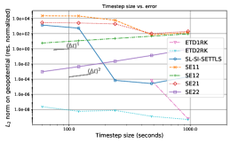
(a) Geostrophic balance

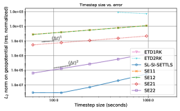
(b) Geostr. balance w/ topography; $h_{0}=100\text{m}$

(c) Geostr. balance w/ topography; $h_{0}=1\text{m}$

(d) Unstable jet

Figure 3: Numerical verification of the convergence order of the schemes considered in this work (normalized $L_{2}$ norm of the error on the geopotential field perturbation vs the time step size). Similar results are obtained with the $L_{\infty}$ norm.

Figure 3 also confirms our hypotheses on the stability and accuracy of semi-Lagrangian exponential methods. These schemes, notably those with a second-order discretization of the nonlinear term, have improved stability properties compared to the Eulerian ones; indeed, ETD2RK and mainly ETD1RK are unstable in most of the simulations. The only simulations in which ETD2RK is stable are those with less important nonlinear effects, meaning that a weaker energy cascade takes place, namely the geostrophically balanced steady-state solution (Figure 3(a)) and the short-run unstable jet simulation (Figure 3(d)). In both simulations, ETD2RK and SE22 outperform the accuracy of the also second-order accurate SL-SI-SETTLS (which develops instabilities in the geostrophic balance test case), reflecting the accurate integration of the linear term by the exponential schemes. On the other hand, SL-SI-SETTLS is more accurate in the geostrophic balance test case with topography (Figures 3(b) and 3(b)), in which the nonlinear effects are more relevant due to the small mean depth $h_{0}$. In this case, although still convergent with the expected accuracy, the semi-Lagrangian exponential schemes produce larger errors. We remark, however, that the observed second-order accuracy of SE22 in this test case confirms the discussion in Section 4 in the sense that the source of the first-order accuracy of SE12 is indeed the discretization of the linear term, and no modification of the discretization of the nonlinear term is required for improving its order of accuracy. Finally, note that some simulations reach an error plateau around $10^{-8}-10^{-9}$, which is a consequence of our formulation considering the geopotential perturbation, $\Phi=\overline{\Phi}+\Phi^{\prime}$, with $\overline{\Phi}$ being several orders of magnitude larger than $\Phi^{\prime}$; therefore, we consider these solutions to have converged.

7.2 Simulation-based stability analysis

As discussed in Section 6, the lack of commutation between the exponential and interpolation operators does not allow us to compare the stability properties of the semi-Lagrangian exponential schemes through a classical linear stability analysis. Therefore, we conduct an empirical simulation-based stability study, as proposed by [25], in which simulations of the governing equations (here, the SWE on the rotating sphere), considering a steady-state solution, are performed in order to estimate the largest eigenvalue of the Jacobian of the approximate time evolution operator, which allows us to estimate the largest growth rate of perturbations to the steady state. This procedure, based on the power method for the estimation of the largest eigenvalue of a matrix, is briefly recalled below. We refer the reader to Appendix B of [25] for details and parameters to be used. Let

(58) $$\boldsymbol{U}^{n+1}=\boldsymbol{G}(\boldsymbol{U}^{n})$$

represent the evolution of a given state vector $\boldsymbol{U}$ between times $t_{n}$ and $t_{n+1}$ using a given time discretization method. Let $\overline{\boldsymbol{U}}$ be a steady state, such that $\boldsymbol{R}^{n}:=\boldsymbol{U}^{n}-\overline{\boldsymbol{U}}$ is the perturbation at time $n$. Through linearization of (58), the perturbation satisfies, to first order

(59) $$\boldsymbol{R}^{n+1}=\boldsymbol{G}^{\prime}(\overline{\boldsymbol{U}})\boldsymbol{R}^{n}$$

As in the power method, the procedure is to iterate over (59). If this method converges, then $\boldsymbol{R}^{n}$ converges to the eigenvector associated with the largest (in absolute value) eigenvalue $\overline{\lambda}$ of $\boldsymbol{G}^{\prime}$. This converged dominant eigenvalue can also be computed, as well as the growth rate $\overline{\nu}:=\log{\overline{\lambda}}/\Delta t$ and the e-folding time $\overline{\tau}$, defined as the time in which $\boldsymbol{R}$ increases by a factor equal to $e$. We have

(60) $$e=\frac{\left\lVert{\boldsymbol{R}^{n}}\right\rVert}{\left\lVert{\boldsymbol{R}^{0}}\right\rVert}=|\overline{\lambda}|^{n}=e^{\overline{\nu}n\Delta t}\implies\overline{\tau}=n\Delta t=\frac{1}{\overline{\nu}}=\frac{\Delta t}{\log\overline{\lambda}}$$

The e-folding time is a relevant parameter, since, even if the scheme is unstable (i.e., $|\overline{\lambda}|>1$), a large e-folding time may indicate that instabilities will remain reasonably small within simulation times used in practical applications, e.g., in numerical weather prediction, such that the time integration scheme can be successfully used in such contexts.

We conduct this stability study by considering the geostrophic balance test case, to which we introduce small initial perturbations to trigger instabilities. The spectral resolution is set to $M=512$, and we compute $\overline{\lambda}$ and $\overline{\tau}$ for various time step sizes and for the various time integration schemes considered here. Results are presented in Figure 4, which only includes simulations for which the iterative procedure described above converges. We do not observe, in this test case, clear differences in the stability behavior depending on the discretization of the linear term in the semi-Lagrangian exponential schemes, with very similar results between SE11 and SE21, and also between SE12 and SE22, i.e., the stability seems to be mostly determined by the discretization of the nonlinear term. The SE12 and SE22 schemes clearly outperform the other methods, including SL-SI-SETTLS, for which the dominant eigenvalue rapidly increases when the time step sizes get larger. Also, unlikely the other schemes, SE12 and SE22 present e-folding times of more than one day for some time step sizes as large as approximately $\Delta t=1000\text{s}$, indicating that simulations can be conducted for relatively large durations with instabilities remaining quite controlled. We recall that no artificial viscosity is considered in this study. Finally, we highlight the unnatural peak on the dominant eigenvalue (corresponding to the abrupt reduction of the e-folding time) of SE12 and SE22 for the tested time step sizes $\Delta t=240\text{s}$ and $\Delta t=480\text{s}$. As described in Section 7.3, this behavior is also observed in the simulation of the unstable jet test case, but the reasons are unknown; it may be caused, e.g., by possible bad behaviors of the exponential functions when computed at time step sizes close to the mentioned values. As identified by [8] through linear stability analyses, exponential integration methods usually have quite erratic stability behaviors, including asymmetric stability regions and discontinuities of the amplification factor as a function of the time step size.

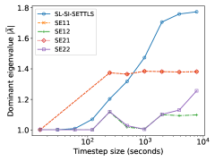
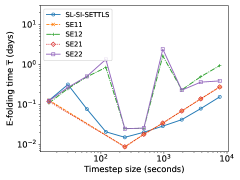
Figure 4: Simulation-based stability analysis considering the geostrophic balanced test case: dominant eigenvalues (left) and corresponding e-folding times (right) as a function of the time step size and the time integration scheme.

7.3 Qualitative comparison

We consider the unstable jet test case to conduct a detailed qualitative comparison of the solutions provided by SE11, SE12, their proposed modifications and SL-SI-SETTLS. This test case is standard in atmospheric modeling research due to its complex dynamics after some days of simulation, and guidelines for evaluating numerical methods applied to it have been proposed by [32]. For this study, we consider a fixed spectral resolution $M=512$ and various time step sizes in the same range $[60,960]$ (s) considered in the convergence analysis. A reference solution is obtained from a simulation using a fourth-order explicit Runge-Kutta method, with $M=1024$ and $\Delta t=2\text{s}$. Results using the Eulerian exponential schemes are not considered due to their highly unstable behavior for all tested time step sizes.

We first present, in Figures 5(a) and 5(b), the kinetic energy spectra produced after six days of simulation by the four semi-Lagrangian exponential schemes, as well as SL-SI-SETTLS, with $\Delta t=120\text{s}$ and $\Delta t=960\text{s}$, and compared to the reference solution. All spectra, including the reference one, present upturned tails, indicating the accumulation of energy on the highest wavenumbers due to the energy cascade, which may lead to instabilities in longer executions if there is not enough dissipation in the numerical scheme [34]; thus, an appropriate application of artificial viscosity or hyperviscosity could be considered in order to mitigate unstable behaviors.

In the case $\Delta t=120\text{s}$, the SE11 scheme presents a clear unstable behavior, with almost the entire spectrum being strongly overamplified. This behavior is partially controlled with the proposed modified discretization of the linear term, and SE21 presents a smaller overamplification of intermediate wavenumbers; concerning SE12 and SE22, their spectra, which almost coincide visually, accurately reproduce the reference one in small and intermediate wavenumbers, but are damped out in the largest ones, indicating a stronger diffusion due to second-order discretization of the nonlinear term; finally, we observe an unstable behavior of SL-SI-SETTLS at the end of the wavenumber spectrum, being outperformed by the semi-Lagrangian exponential schemes using a second-order discretization of the nonlinear term.

When the larger time step size $\Delta t=960\text{s}$ is considered, all time integration schemes present overamplifications of at least a portion of the wavenumber spectrum, notably SL-SI-SETTLS. The most stable simulation is provided by our proposed second-order scheme SE22, whose spectrum presents only a small peak at medium wavenumbers, being able to well reproduce the reference one at the large scales and remaining below it at the fine ones. Note that SE12, which provides nearly identical results to SE22 when $\Delta t=120\text{s}$, has now a much more pronounced unstable behavior, with overamplification of almost the entire spectrum.

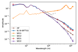
(a) $\Delta t=120\text{s}$, 6 days

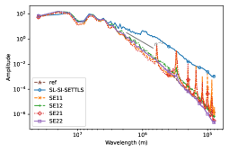
(b) $\Delta t=960\text{s}$, 6 days

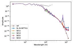
(c) $\Delta t=240\text{s}$, 1 day

Figure 5: Kinetic energy spectra, truncated at resolution $M=512$, for the unstable jet test case.

We remark that, among the tested time step sizes, the four semi-Lagrangian exponential schemes present very early unexpected unstable behaviors when $\Delta t$ is chosen around $240$s and $480$s, which has been identified in the stability analysis presented above (Figure 4). Figure 5(c) illustrates the kinetic energy spectrum after a single day of simulation (i.e., long before the vortices start to appear), in which we observe unnatural peaks in the spectrum of the solutions of the semi-Lagrangian exponential methods. This behavior is not observed, at least not this early, for reasonably larger time step, e.g., $\Delta t=960\text{s}$ as seen above. The reasons for this are not yet understood. A possible explanation is that one or more of the exponential functions $\varphi_{k}$, $\psi_{k}$ may be not too well behaved when computed at $\Delta t\boldsymbol{L}$, with $\boldsymbol{L}$ defined by the parameters of the SWE on the rotating sphere and $\Delta t$ around the values mentioned above. Therefore, the use of artificial viscosity or hyperviscosity would be required to ensure further stability. This is studied in Section 7.5.

Some of the vorticity fields corresponding to the spectra illustrated in Figures 5(a) and 5(b). are presented in Figure 6. With $\Delta t=120\text{s}$, it is clear that both SE12 and SE22 provide similar results, visually close to the reference one and outperforming SL-SI-SETTLS, which produces small-scale oscillations that degrade the accuracy of the solution. With $\Delta t=960\text{s}$, the larger amount of numerical diffusion seems to improve the quality of the solution provided by SL-SI-SETTLS in most of the spatial domain, but large localized errors are still visible. The most important loss of accuracy is experimented with SE12, with clear deformations of the vortices and small-scale oscillating errors starting to dominate the solution. These small oscillations are also present in the solution of SE22, but with a much smaller amplitude, such that the profile of the reference solution is still well represented.

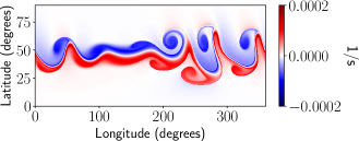
(a) Reference, $\Delta t=2\text{s}$

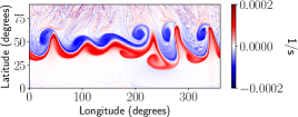
(b) SL-SI-SETTLS, $\Delta t=120\text{s}$

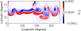
(c) SL-SI-SETTLS, $\Delta t=960\text{s}$

(d) SE12, $\Delta t=120\text{s}$

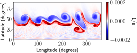
(e) SE12, $\Delta t=960\text{s}$

(f) SE22, $\Delta t=120\text{s}$

(g) SE22, $\Delta t=960\text{s}$

Figure 6: Potential vorticity field after six days of simulation in the northern hemisphere, using selected integration schemes and time step sizes, compared to the reference solution obtained from a fourth-order explicit Runge-Kutta method with $M=1024$ and $\Delta t=2\text{s}$.

We now compare the obtained results using the guidelines provided by [32] for the study of the unstable jet test case. First, we present, in Figure 7, the contour lines of the potential vorticity field of each simulation after six days on the region $[240^{\circ},300^{\circ}]\times[15^{\circ},75^{\circ}]$, compared to the reference solution provided by [32], which is obtained considering a spectral resolution $M=2730$. The potential vorticity is defined by $\xi_{p}:=\xi_{a}/h$, where $\xi_{a}:=2\Omega\sin\theta+\xi=f+\xi$ is the absolute vorticity. For the sake of conciseness, among the semi-Lagrangian exponential methods, only results produced by SE12 and SE22 are presented. With $\Delta t=120\text{s}$, small-scale oscillating errors are observed in the solution produced by SL-SI-SETTLS, which is also slightly displaced w.r.t. the reference one; both SE12 and SE22 produce solutions close to the reference contour, with a better representation of some small-scale details by the latter scheme. With $\Delta t=960\text{s}$, small-scale and displacement errors are still present in the SL-SI-SETTLS solution; concerning SE22, it still represents well the general profile and position of the reference solution, indicating smaller dispersion errors compared to the other schemes, but clear oscillations reveal the formation of unstable behaviors; finally, the solution of SE12 is strongly deteriorated both in shape and position.

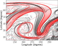
(a) SL-SI-SETTLS, $\Delta t=120\text{s}$

(b) SE12, $\Delta t=120\text{s}$

(c) SE22, $\Delta t=120\text{s}$

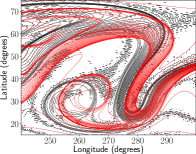
(d) SL-SI-SETTLS, $\Delta t=960\text{s}$

(e) SE12, $\Delta t=960\text{s}$

(f) SE22, $\Delta t=960\text{s}$

Figure 7: Contour lines of the potential vorticity field after six days of simulation of the unstable jet test case, using selected time integration methods (black lines), compared to the reference solution provided by [32] (red lines). Contour levels are separated by $0.2\Omega/\overline{h}$.

[32] also propose a set of metrics for a quantitative evaluation of the convergence of numerical solutions of the unstable jet test case. Among them, the maximum absolute value of the vorticity ($\left\lVert{\xi}\right\rVert_{\infty}$) and the relative error of the maximum potential vorticity ($(\left\lVert{\xi_{p}}\right\rVert_{\infty}-\left\lVert{(\xi_{p})_{0}}\right\rVert_{\infty})/\left\lVert{(\xi_{p})_{0}}\right\rVert_{\infty}$, where $(\xi_{p})_{0}$ is the initial potential vorticity), are identified to be proper convergence diagnostics. These quantities at every day of simulation are plotted in Figure 8 for the solutions computed with SL-SI-SETTLS, SE12 and SE22, being compared to the reference solution, as well as to reference values provided by [32] at day 5. With the small time step $\Delta t=120\text{s}$, the semi-Lagrangian exponential schemes outperform SL-SI-SETTLS, and they even provide better approximations to the reference value of the potential vorticity deviation compared to our reference solution, which, as discussed above, presents a slightly unstable behavior at the very end of the wavenumber spectrum. Under the larger time step $\Delta t=960\text{s}$, the instabilities of SE12 are clear, with a fast divergence from the reference values from the first day of simulation; SL-SI-SETTLS and SE22 have a much later divergence, mainly the latter, which stays relatively close to our reference solution until day 6 or 7.

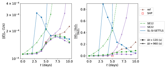
Figure 8: Evolution of diagnostic quantities in the unstable jet test case, measured at every day of simulation. “ref” indicates the reference solution (4th order explicit Runge-Kutta, with $M=1024$ and $\Delta t=2\text{s}$) and “SHP” indicates the reference values provided by Scott, Harris and Polvani [32] at day 5. Left: maximum absolute value of the vorticity field; right: deviation of the maximum absolute value of the potential vorticity field.

7.4 Evaluation of computational cost

We compare, in Table 2, the wall-clock times for the integration of the simulations whose kinetic energy spectra are presented in Figures 5(a) and 5(b). Each simulation is executed with threaded spatial parallelization in 16 physical cores of Intel Xeon Gold 6130 2.10GHz in the GRICAD cluster from the University of Grenoble Alpes. As expected from the complexity analysis depicted in Table 1, the proposed modification of the discretization of the linear term strongly increases the computing time of the semi-Lagrangian exponential schemes, by factors ranging approximately between 40% and 65%. However, the proposed SE22 scheme, which provided the most stable and accurate results, presents a comparable cost with the well-established SL-SI-SETTLS. Moreover, the evaluation of the exponential functions is not fully optimized in our implementation, such that further wall clock time improvements could be obtained.

	SL-SI-SETTLS	SE11	SE21	SE12	SE22
$\Delta t=120\text{s}$	1378	757	1051	1244	1538
$\Delta t=960\text{s}$	178	97	132	149	190

Table 2: Approximate wall clock times (in seconds) for the integration of the unstable jet test case (10 days of simulation) by selected schemes.

7.5 Application of artificial viscosity and hyperviscosity

No artificial viscosity or hyperviscosity was applied in the numerical simulations presented above. Although relatively stable simulations were indeed obtained, mainly with the proposed SE22 scheme, we identified some indications that viscosity approaches should be used for further stability, e.g., the lack of convergence in the geostrophic balance test case (Figure 3(a)), the upturned tails at the end of the wavenumber spectra (Figure 5) and the localized peaks in the spectra of semi-Lagrangian exponential methods when specific time step sizes are used (Figures 4 and 5(c)). The goal of this section is to verify if artificial viscosity and hyperviscosity approaches are able to mitigate these issues and to identify a compromise between stability and accuracy when choosing the viscosity parameters, namely the viscosity order $q$ and the viscosity coefficient $\nu$. In practice, artificial viscosity and/or numerical diffusion inherent to the discretization schemes are required in operational global atmospheric circulation models [37]. Ideally, one would use higher-order viscosity approaches ($q>2$), in order to damp only the largest wavenumbers (the ones in which instabilities may be triggered first due to the energy cascade induced by the nonlinearity of the problem) and preserve the largest ones, thus maintaining relatively high accuracy. Fourth-, sixth- and eight-order hyperviscosity approaches are usually considered in models using spectral discretization [17]; for instance, the spectral models IFS-ECMWF [10] and GFS-NCEP/NOAA [23] use respectively fourth- and eight-order viscosities. The determination of viscosity coefficients depends on the spectral resolution and the damping timescale, i.e., the time necessary for damping a given wavenumber by a given fraction, which varies between units and tenths of hours. We refer the reader to Appendix A of [4] for details and to the references therein for reports of viscosity parameters usually applied in spectral methods for atmospheric circulation models.

In all simulations presented here, the viscosity term $\boldsymbol{L}_{\nu}$ is solved at the end of each time step using a first-order backward Euler-scheme. We start with the 7 days simulation of the geostrophic balance test case, in which the majority of the tested time stepping schemes did not present a stable behavior (Figure 3(a)). We consider two viscosity configurations, namely $(q,\nu)=(4,10^{15})$ and $(q,\nu)=(6,10^{24})$, with $\nu$ expressed in $\text{m}^{q}\text{s}^{-1}$. No viscosity is used for computing the reference solutions. Figure 9 reveals that both approaches can ensure the stability of the tested schemes, and the expected convergence orders are verified. In the case of the fourth-order viscosity, however, the damping of a larger range of wavenumbers degrades the quality of the solution, whose relative error w.r.t. the reference stagnates at approximately $10\%$. Smaller values of fourth-order viscosity are not able to stabilize all simulations. Using a sixth-order approach, this impact on the accuracy is much weaker, with the relative error converging to approximately $0.001\%$, and only the first-order Eulerian exponential method still presents some instabilities. We also observe that SL-SI-SETTLS and the Eulerian exponential schemes converge much faster to this final error compared to the semi-Lagrangian exponential methods; it is worth noting, however, that SE12 and SE22 do not require artificial viscosity in this test case to present a stable and convergent behavior.

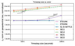
(a) $(q,\nu)=(4,10^{15})$

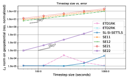
(b) $(q,\nu)=(6,10^{24})$

Figure 9: Normalized $L_{2}$ norm of the error on the geopotential field perturbation vs the time step size for the geostrophic balance test case after seven days of simulation, using artificial viscosity approaches.

We now consider the unstable jet test case with $\Delta t=240\text{s}$, for which clear instabilities were observed in the integration of the semi-Lagrangian exponential schemes, with $(q,\nu)=(4,10^{15})$ and $(q,\nu)=(6,10^{24})$. Smaller viscosity coefficients were not able to fully prevent the formation of peaks in the kinetic energy spectra. As presented in Figure 10, both viscosity configurations ensure stability at the cost of important damping of the highest wavenumber modes (and stronger damping of intermediate modes with the fourth-order viscosity), with very close results for all tested time integration methods. As illustrated in Figure 11 for the SE22 scheme (qualitatively similar results are obtained using SE12 or SL-SI-SETTLS), the sixth-order viscosity produces a better approximation to the reference solution provided by [32].

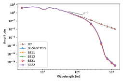
(a) $(q,\nu)=(4,10^{15})$

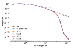
(b) $(q,\nu)=(6,10^{24})$

Figure 10: Kinetic energy spectra after six days of simulation, with $\Delta t=240\text{s}$ (and $\Delta t=2\text{s}$ for the reference solution), truncated at the resolution $M=512$, for the unstable jet case with artificial viscosity.

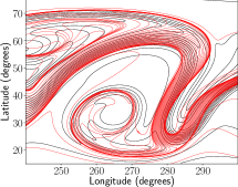
(a) $(q,\nu)=(4,10^{15})$

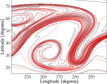
(b) $(q,\nu)=(6,10^{24})$

Figure 11: Contour lines of the potential vorticity field after six days of simulation of the unstable jet test case with artificial viscosity, using the SE22 scheme and $\Delta t=240\text{s}$ (black lines), compared to the reference solution provided by [32] (red lines). Contour levels are separated by $0.2\Omega/\overline{h}$.

By comparing these results with the simulations without viscosity (Figure 7), we observe that SE22 with $\Delta t=120\text{s}$, $\nu=0$ is qualitatively superior to the simulation with $\Delta t=240\text{s}$ and $(q,\nu)=(6,10^{24})$, but the latter outperforms the simulation with $\Delta t=960\text{s}$, $\nu=0$, which presents several small-scale oscillations despite a relatively stable simulation compared to other time integration schemes. On the other hand, SL-SI-SETTLS and SE12 clearly benefit from the use of artificial viscosity, with considerably more stable and accurate results compared to the inviscid case with both $\Delta t=120\text{s}$ and $\Delta t=960\text{s}$ (in the case of SL-SI-SETTLS) or $\Delta t=960\text{s}$ (in the case of SE12).

8 Conclusion

Semi-Lagrangian exponential methods, proposed by [24], have a potential for application in atmospheric circulation models, since they have enhanced stability compared to Eulerian exponential schemes and, contrary to traditional semi-Lagrangian methods, are able to integrate the linear terms very accurately; therefore, this class of time stepping scheme is more suitable for the integration of advection-dominated models containing stiff linear terms. The work presented here aimed to extend [24] in several aspects: first, we identified and explained the accuracy limitations of their methods, showing that the combination of exponential and interpolation operators adopted in the discretization of the linear term produces a first-order leading term in the truncation error. Second, inspired by this initial study, we proposed a new method, with an alternative discretization of the linear term, leading to an effective second-order accuracy. Also, we conducted a detailed stability study comparing several Eulerian and semi-Lagrangian methods, both through a linear stability analysis and an empirical simulation-based stability study, which was required because the standard stability analysis is not able to provide detailed insights in the stability of semi-Lagrangian exponential schemes. Finally, while [24] developed their work in the context of the SWE on the biperiodic plane, we applied the schemes to the integration of the SWE on the rotating sphere, thus providing results that are more closely related to real-world operational atmospheric circulation models.

Promising results were obtained using the proposed second-order semi-Lagrangian exponential scheme. Its theoretical convergence order was confirmed in several benchmark test cases, and, considering the especially challenging unstable jet simulation, it proved to be more stable and accurate than Eulerian exponential schemes, other semi-Lagrangian exponential schemes and the well-established second-order SL-SI-SETTLS, even without the use of artificial viscosity approaches, which is a consequence of the combined accurate integration of the stiff linear terms and the semi-Lagrangian treatment of the advection. The proposed scheme also has improved accuracy w.r.t. SL-SI-SETTLS in simulations dominated by linear processes; however, it is outperformed by this latter method (if stable) when nonlinear effects are more important. In terms of computational cost, a drawback of the proposed method is its higher complexity compared to the previously formulated first-order semi-Lagrangian exponential schemes, as a consequence of the splitting of the exponential operator applied to the linear term, which is required to achieve second-order accuracy. We highlight, however, that this larger cost can be mitigated by a straightforward computation of matrix exponentials, by combining a spectral discretization with a convenient arrangement of the terms of the governing equations, and by precomputing these exponential terms, which is possible in simulations with a constant time step size. Also, the observed wall-clock times are comparable to those of SL-SI-SETTLS, which is used in operational atmospheric circulation models; therefore, our proposed method seems to be a competitive candidate for operational applications.

Important aspects still need to be considered in future work for further improvement of semi-Lagrangian exponential methods. As illustrated in the numerical simulations, these schemes presented unexpected unstable behaviors in a specific range of time step sizes, which can possibly be caused by badly behaved exponential functions; even if these issues have been easily avoided by using high-order artificial viscosity, with little damage to the accuracy of the numerical solution, a more detailed understanding needs to be achieved. Also, higher-order semi-Lagrangian exponential schemes can be formulated to achieve improved accuracy in simulations dominated by nonlinearities; from the truncation error analyses conducted here, they could probably be obtained in a quite straightforward way following the derivation of higher-order Eulerian exponential methods by [7] and using the proposed split discretization of the linear term. Finally, applications to more complex atmospheric models would be a natural and challenging extension of this work.

References

- [1] L. Bonaventura, Exponential integrators for multiple time scale problems of environmental fluid dynamics. Innovative Integrators Workshop 27-30 October 2010. Universität Innsbruck, Austria.
- [2] M. Brachet, L. Debreu, and C. Eldred, Comparison of exponential integrators and traditional time integration schemes for the shallow water equations, Applied Numerical Mathematics, 180 (2022), pp. 55–84, https://doi.org/10.1016/j.apnum.2022.05.006.
- [3] T. Buvoli and M. L. Minion, On the stability of exponential integrators for non-diffusive equations, Journal of Computational and Applied Mathematics, 409 (2022), p. 114126, https://doi.org/10.1016/j.cam.2022.114126.
- [4] J. G. Caldas Steinstraesser, P. d. S. Peixoto, and M. Schreiber, Parallel-in-time integration of the shallow water equations on the rotating sphere using parareal and mgrit, Jan. 2024, https://doi.org/10.1016/j.jcp.2023.112591, http://dx.doi.org/10.1016/j.jcp.2023.112591.
- [5] J. Certaine, The solution of ordinary differential equations with large time constants, Mathematical methods for digital computers, (1960), pp. 128–132.
- [6] C. Clancy and J. A. Pudykiewicz, On the use of exponential time integration methods in atmospheric models, Tellus A: Dynamic Meteorology and Oceanography, 65 (2013), p. 20898, https://doi.org/10.3402/tellusa.v65i0.20898.
- [7] S. Cox and P. Matthews, Exponential time differencing for stiff systems, Journal of Computational Physics, 176 (2002), pp. 430–455, https://doi.org/https://doi.org/10.1006/jcph.2002.6995.
- [8] N. Crouseilles, L. Einkemmer, and J. Massot, Exponential methods for solving hyperbolic problems with application to collisionless kinetic equations, Journal of Computational Physics, 420 (2020), p. 109688, https://doi.org/10.1016/j.jcp.2020.109688.
- [9] D. Durran, Numerical methods for fluid dynamics : with applications to geophysics, Springer, New York, 2010.
- [10] ECMWF and P. White, IFS Documentation CY25R1 - Part III: Dynamics and Numerical Procedures, (2003), https://doi.org/10.21957/KBHDQL7MN.
- [11] J. Galewsky, R. K. Scott, and L. M. Polvani, An initial-value problem for testing numerical models of the global shallow-water equations, Tellus A: Dynamic Meteorology and Oceanography, 56 (2004), pp. 429–440, https://doi.org/10.3402/tellusa.v56i5.14436.
- [12] S. Gaudreault and J. A. Pudykiewicz, An efficient exponential time integration method for the numerical solution of the shallow water equations on the sphere, Journal of Computational Physics, 322 (2016), pp. 827–848, https://doi.org/10.1016/j.jcp.2016.07.012.
- [13] T. S. Haut, T. Babb, P. G. Martinsson, and B. A. Wingate, A high-order time-parallel scheme for solving wave propagation problems via the direct construction of an approximate time-evolution operator, IMA Journal of Numerical Analysis, 36 (2015), pp. 688–716, https://doi.org/10.1093/imanum/drv021.
- [14] M. Hochbruck and A. Ostermann, Exponential integrators of rosenbrock-type, Oberwolfach Reports, 3 (2006), pp. 1107–1110.
- [15] M. Hochbruck and A. Ostermann, Exponential integrators, Acta Numerica, 19 (2010), pp. 209–286, https://doi.org/10.1017/s0962492910000048.
- [16] M. Hortal, The development and testing of a new two‐time‐level semi‐lagrangian scheme (settls) in the ecmwf forecast model, Quarterly Journal of the Royal Meteorological Society, 128 (2002), p. 1671–1687, https://doi.org/10.1002/qj.200212858314.
- [17] C. Jablonowski and D. L. Williamson, The pros and cons of diffusion, filters and fixers in atmospheric general circulation models, in Numerical Techniques for Global Atmospheric Models, P. Lauritzen, C. Jablonowski, M. Taylor, and R. Nair, eds., Springer Berlin Heidelberg, 2011, ch. 13, pp. 381–493.
- [18] J. D. Lawson, Generalized runge-kutta processes for stable systems with large lipschitz constants, SIAM Journal on Numerical Analysis, 4 (1967), p. 372–380, https://doi.org/10.1137/0704033.
- [19] M. S. Longuet-Higgins, The eigenfunctions of laplace’s tidal equations over a sphere, Philosophical Transactions of the Royal Society A: Mathematical, Physical and Engineering Sciences, 262 (1968), p. 511–607, https://doi.org/10.1098/rsta.1968.0003.
- [20] V. T. Luan, J. A. Pudykiewicz, and D. R. Reynolds, Further development of efficient and accurate time integration schemes for meteorological models, Journal of Computational Physics, 376 (2019), pp. 817–837, https://doi.org/10.1016/j.jcp.2018.10.018.
- [21] G. Mengaldo, A. Wyszogrodzki, M. Diamantakis, S.-J. Lock, F. X. Giraldo, and N. P. Wedi, Current and emerging time-integration strategies in global numerical weather and climate prediction, Archives of Computational Methods in Engineering, 26 (2018), pp. 663–684, https://doi.org/10.1007/s11831-018-9261-8.
- [22] B. V. Minchev and W. M. Wright, A review of exponential integrators for first-order semi-linear problems, tech. report, Norwegian University of Science and Technology, 2005.
- [23] U. N. Oceanic and A. A. N. . N. C. for Environmental Prediction (NCEP), Global Forecast System - Global Spectral Model (GSM) - V13.0.2. https://vlab.noaa.gov/web/gfs/documentation, May 2016.
- [24] P. S. Peixoto and M. Schreiber, Semi-Lagrangian Exponential Integration with Application to the Rotating Shallow Water Equations, SIAM Journal on Scientific Computing, 41 (2019), pp. B903–B928, https://doi.org/10.1137/18M1206497, https://arxiv.org/abs/https://doi.org/10.1137/18M1206497.
- [25] P. S. Peixoto, J. Thuburn, and M. J. Bell, Numerical instabilities of spherical shallow‐water models considering small equivalent depths, Quarterly Journal of the Royal Meteorological Society, 144 (2017), p. 156–171, https://doi.org/10.1002/qj.3191.
- [26] J. A. Pudykiewicz and C. Clancy, Convection experiments with the exponential time integration scheme, Journal of Computational Physics, 449 (2022), p. 110803, https://doi.org/10.1016/j.jcp.2021.110803.
- [27] G. Rainwater, K. C. Viner, and P. A. Reinecke, Exponential time integration for 3d compressible atmospheric models, 2023, https://arxiv.org/abs/2309.09869.
- [28] Y. Saad, Variations on arnoldi’s method for computing eigenelements of large unsymmetric matrices, Linear Algebra and its Applications, 34 (1980), p. 269–295, https://doi.org/10.1016/0024-3795(80)90169-x.
- [29] N. Schaeffer, Efficient spherical harmonic transforms aimed at pseudospectral numerical simulations, Geochemistry, Geophysics, Geosystems, 14 (2013), p. 751–758, https://doi.org/10.1002/ggge.20071.
- [30] M. Schreiber and R. Loft, A parallel time integrator for solving the linearized shallow water equations on the rotating sphere, Numerical Linear Algebra with Applications, 26 (2018), https://doi.org/10.1002/nla.2220.
- [31] M. Schreiber, N. Schaeffer, and R. Loft, Exponential integrators with parallel-in-time rational approximations for the shallow-water equations on the rotating sphere, Parallel Computing, 85 (2019), p. 56–65, https://doi.org/10.1016/j.parco.2019.01.005.
- [32] R. K. Scott, L. M. Harris, and L. M. Polvani, A test case for the inviscid shallow‐water equations on the sphere, Quarterly Journal of the Royal Meteorological Society, 142 (2015), p. 488–495, https://doi.org/10.1002/qj.2667.
- [33] V. V. Shashkin and G. S. Goyman, Semi-lagrangian exponential time-integration method for the shallow water equations on the cubed sphere grid, Russian Journal of Numerical Analysis and Mathematical Modelling, 35 (2020), pp. 355–366, https://doi.org/10.1515/rnam-2020-0029.
- [34] W. C. Skamarock, Evaluating mesoscale nwp models using kinetic energy spectra, Monthly Weather Review, 132 (2004), p. 3019–3032, https://doi.org/10.1175/mwr2830.1.
- [35] A. Staniforth and J. Côté, Semi-lagrangian integration schemes for atmospheric models—a review, Monthly Weather Review, 119 (1991), pp. 2206–2223, https://doi.org/10.1175/1520-0493(1991)119<2206:slisfa>2.0.co;2.
- [36] C. Temperton, Treatment of the coriolis terms in semi-lagrangian spectral models, Atmosphere-Ocean, 35 (1997), pp. 293–302, https://doi.org/10.1080/07055900.1997.9687353.
- [37] J. Thuburn, Numerical wave propagation on the hexagonal c-grid, Journal of Computational Physics, 227 (2008), p. 5836–5858, https://doi.org/10.1016/j.jcp.2008.02.010.
- [38] S. Vasylkevych and N. Žagar, A high‐accuracy global prognostic model for the simulation of rossby and gravity wave dynamics, Quarterly Journal of the Royal Meteorological Society, 147 (2021), p. 1989–2007, https://doi.org/10.1002/qj.4006.
- [39] D. L. WILLIAMSON, The evolution of dynamical cores for global atmospheric models, Journal of the Meteorological Society of Japan. Ser. II, 85B (2007), p. 241–269, https://doi.org/10.2151/jmsj.85b.241.
- [40] D. L. Williamson, J. B. Drake, J. J. Hack, R. Jakob, and P. N. Swarztrauber, A standard test set for numerical approximations to the shallow water equations in spherical geometry, Journal of Computational Physics, 102 (1992), pp. 211–224, https://doi.org/10.1016/s0021-9991(05)80016-6.