Hybridizable discontinuous Galerkin methods for solving the two-fluid plasma model

Abstract

The two-fluid plasma model has a wide range of timescales which must all be numerically resolved regardless of the timescale on which plasma dynamics occurs. The answer to solving numerically stiff systems is generally to utilize unconditionally stable implicit time advance methods. Hybridizable discontinuous Galerkin (HDG) methods have emerged as a powerful tool for solving stiff partial differential equations. The HDG framework combines the advantages of the discontinuous Galerkin (DG) method, such as high-order accuracy and flexibility in handling mixed hyperbolic/parabolic PDEs with the advantage of classical continuous finite element methods for constructing small numerically stable global systems which can be solved implicitly. In this research we quantify the numerical stability conditions for the two-fluid equations and demonstrate how HDG can be used to avoid the strict stability requirements while maintaining high order accurate results.

35L60, 65M12, 65M60

1 Introduction

The two-fluid plasma model is a very numerically stiff PDE system. The model couples together the time evolution of an ion fluid, an electron fluid, and Maxwell’s equations. As a result the characteristic dynamics leads to timescales which can span two to four orders of magnitude, include both the speed of light and various electron wave modes along with ion fluid dynamics. The large span of timescales makes the PDE system a prime candidate for being solved using implicit time stepping. However, there are several challenges in actualizing an implicit numerical solution. The system is a mixed advection-diffusion-reaction system consisting of six scalar fields and four vector fields with a nominal 18 components to be evolved in 3D. The hyperbolic characteristics makes using standard continuous Galerkin (CG) methods challenging, and traditional discontinuous Galerkin (DG) methods are not typically amenable with implicit time stepping schemes[20]. One solution is the use of hybridizable discontinuous Galerkin (HDG) methods[4]. These methods are designed to allow the implicit DG discretization to be partitioned into three distinct phases, reducing the largest global system solve size as well as producing a scheme which maintains local compactness. Nguyen and Peraire[19] have demonstrated the applicability of HDG to a wide variety of linear and non-linear PDEs, including Stoke’s equations, incompressible Navier-Stokes equations, and the compressible Euler equations. They demonstrated that the method can be formulated to achieve optimal $k+1$ orders of convergence, where $k$ is the polynomial basis order. Lee et al.[15] demonstrated that the linearized incompressible resistive MHD equations can be solved using HDG, opening the door to modeling basic plasma systems using HDG. In this paper we present techniques and tools for expanding the applicability of HDG to large coupled PDE systems such as the two-fluid plasma model using HDG. Section 2 introduces the two-fluid plasma system to be solved, and discusses challenges associated with solving this particular system using explicit Runge-Kutta discontinuous Galerkin (RKDG). LABEL:sec:hdg presents the HDG discretization method and practical implementation details required for solving complex PDE systems. Section 4 presents the verification of the implementation by checking the convergence rates on linear systems. Finally Section 5 presents results of solving the two-fluid plasma using HDG.

2 The two-fluid plasma model

The two-fluid plasma model is a subset of the general multi-fluid 5N-moment plasma model[22]. This model treats each constituent particle species type as their own fluid species. Coupling between the species occurs via local inter-species collisions and long-range electromagnetic field coupling described using Maxwell’s Equations. For the two-fluid model a single positively charge ion species is coupled to an electron species. The exact form being considered for this paper is given by

(1)

where $\rho_{\alpha}$, $\vec{p}_{\alpha}$, $U_{\alpha}$ are the mass, momentum, and internal energy densities of species $\alpha$ and $\mu_{c}$, $\kappa_{c}$, $R_{c}$, $Q_{c}$ are constants for the viscosity, thermal diffusivity, interspecies momentum transfer, and interspecies heat transfer coefficients respectively. $m_{\alpha}$, $Z_{\alpha}$, and $\gamma$ describe the mass, charge state, and heat capacity ratio of species $\alpha$. For the two-fluid model $\alpha$ is either $i$ for ions or $e$ for electrons, while $\beta$ is the other species. The following additional substitutions are used to simplify the notation:

(2) $$\vec{u}_{\alpha}=\frac{\vec{p}_{\alpha}}{\rho_{\alpha}}$$

(3) $$P_{\alpha}=U_{\alpha}(\gamma-1)$$

(4) $$T_{\alpha}=\frac{m_{\alpha}P_{\alpha}}{\rho_{\alpha}}$$

(5) $$\rho_{c}=\frac{Z_{i}}{m_{i}}\rho_{i}+\frac{Z_{e}}{m_{e}}\rho_{e}$$

(6) $$\vec{j}=\frac{Z_{i}}{m_{i}}\vec{p}_{i}+\frac{Z_{e}}{m_{e}}\vec{p}_{e}$$

The plasma fluid equations are then coupled to EM fields via Maxwell’s equations. These are evolved using For a large PDE system such as the two-fluid plasma model, deriving correct analytical Jacobians by hand is practically impossible due to the large number of non-zero entries. For the two-fluid plasma system this requires at least 1047 unique non-zero entries, before taking into account boundary conditions which may double or triple the number of analytical Jacobian non-zeroes. To solve this problem the Jacobian along with the rest of the HDG code is generated using SymPy[17], a symbolic computer algebra system. The tool is capable of automatically detecting and eliminating unused degrees of freedom and handles multiple subdomains/boundary conditions. The generated HDG code is coupled with a diagonally implicit Runge-Kutta[11] temporal solver, and parallelized on CPUs using MPI.

3.2 Face-oriented numerical flux

A key requirement for the HDG numerical flux is that from the perspective of any element the numerical flux must be a function of only the DOFs inside the element and the DOF on the neighboring face. Each face is assigned a local normal, tangent, and binormal. As a result the face normal will point outwards for one element, while for the adjacent neighboring element it points inwards. The non-uniqueness of the tangent and binormal directions is not an issue so long as they are chosen such that $\hat{t}=\hat{n}\times\hat{b}$. Vector and tensor quantities are appropriately rotated to the face coordinate system for computing numerical fluxes.

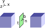
Figure 3: Global and face-oriented coordinate systems

Computing the numerical flux becomes

(58) $$(\stackrel{{\scriptstyle\leftrightarrow}}{{\boldsymbol{T}}}\hat{n})^{*}=\pm\vec{T}_{n}^{*}$$

Depending on the given system this could potentially lead to a reduction of face DOF[1]. For example, take the linear diffusion equation

$$\partial_{t}\phi-\operatorname{\nabla{\cdot}}\vec{\gamma}=$$

(59) $$\vec{\gamma}=\operatorname{\nabla}\phi$$

The numerical fluxes chosen are the class of central fluxes of the form

(60) $$(\stackrel{{\scriptstyle\leftrightarrow}}{{\boldsymbol{T}}}\hat{n})^{*}=\stackrel{{\scriptstyle\leftrightarrow}}{{\boldsymbol{T}}}_{\lambda}\hat{n}+\tau(\vec{q}^{-}-\vec{\lambda})$$

For the linear diffusion equation this expands to

(61) $$(\stackrel{{\scriptstyle\leftrightarrow}}{{\boldsymbol{T}}}\hat{n})^{*}=\begin{bmatrix}\lambda_{\vec{\gamma}}\cdot\hat{n}^{-}+\tau(q^{-}_{\phi}-\lambda_{\phi})\\ -\lambda_{\phi}\stackrel{{\scriptstyle\leftrightarrow}}{{\boldsymbol{I}}}\hat{n}^{-}+\tau(q^{-}_{\vec{\gamma}}-\lambda_{\vec{\gamma}})\end{bmatrix}$$

where $\tau>0$ is a user chosen constant. Note that in practice so long as $\tau\approx 1$ the method will converge at the same rate. In a global coordinate system this expands to

(62) $$(\stackrel{{\scriptstyle\leftrightarrow}}{{\boldsymbol{T}}}\hat{n})^{*}=\begin{bmatrix}\lambda_{\gamma_{x}}\hat{n}^{-}_{x}+\lambda_{\gamma_{y}}\hat{n}^{-}_{y}+\lambda_{\gamma_{z}}\hat{n}^{-}_{z}+\tau(q^{-}_{\phi}-\lambda_{\phi})\\ \begin{bmatrix}-\lambda_{\phi}\hat{n}^{-}_{x}+\tau(q^{-}_{\gamma_{x}}-\lambda_{\gamma_{x}})\\ -\lambda_{\phi}\hat{n}^{-}_{y}+\tau(q^{-}_{\gamma_{y}}-\lambda_{\gamma_{y}})\\ -\lambda_{\phi}\hat{n}^{-}_{z}+\tau(q^{-}_{\gamma_{z}}-\lambda_{\gamma_{z}})\end{bmatrix}\end{bmatrix}$$

which requires four element scalar fields and four face scalar fields. In a rotated frame this can be simplified to

(63) $$(\stackrel{{\scriptstyle\leftrightarrow}}{{\boldsymbol{T}}}\hat{n})^{*}=\begin{bmatrix}\pm\lambda_{\gamma_{n}}+\tau(q^{-}_{\phi}-\lambda_{\phi})\\ \begin{bmatrix}\mp\lambda_{\phi}+\tau(q^{-}_{\gamma_{n}}-\lambda_{\gamma_{n}})\\ 0\\ 0\end{bmatrix}\end{bmatrix}$$

eliminating two face scalar fields. For the two-fluid plasma model with either mixed parabolic-hyperbolic cleaning or purely parabolic cleaning this rotation scheme requires a total of 42 element and 34 face scalar fields, eliminating eight face scalar fields from the non-rotated scheme.

4 Validation of convergence rates for various linear systems

Convergence is evaluated for several model PDE systems including the linear advection, diffusion equation, and wave equation. In all cases periodic boundary conditions are applied on a 3D cube domain $\vec{r}\in[0,1]^{3}$ and $t\in[0,0.1]$ with a fixed $\Delta t=5\times 10^{-3}$. The error is compared against the analytical solution $a_{a}$ using an $8^{3}$ tensor product Gauss-Lobatto quadrature to compute the L-2 error integral

(64) $$\epsilon=\sqrt{\int(q_{h}-q_{a})^{2}dV}$$

The linear advection system is defined by

$$\partial_{t}q+\operatorname{\nabla{\cdot}}(\vec{a}q)=$$

(65) $$\vec{a}^{T}=\begin{bmatrix}1&\frac{1}{2}&2\end{bmatrix}$$

(66) $$q_{a}(x,y,z,t)=\cos(2\pi(x-a_{x}t))\cos(2\pi(y-a_{y}t))\cos(2\pi(z-a_{z}t))$$

Figure 4 demonstrates that the linear advection system converges at the expected optimal $O(N+1)$ rates.

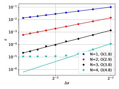
Figure 4: L-2 error norms for the linear advection equation converge at the expected optimal $O(N+1)$ rates for degree $N$ basis. The observed $10^{-5}$ minimum error is from the temporal discretization error.

Note that at small $\Delta x$ and high basis order the simulation reaches a saturation floor of $10^{-5}$ from the temporal discretization error. This can be reduced by choosing a smaller $\Delta t$ or more accurate temporal discretization method.

The linear diffusion system is defined by

$$\partial_{t}q-\operatorname{\nabla{\cdot}}(k\operatorname{\nabla}q)=$$

This can be decomposed into a coupled system of first order equations to fit the form of LABEL:eq:hdg_prototype as

$$\partial_{t}q-\operatorname{\nabla{\cdot}}(k\vec{u})=$$

(67) $$\vec{u}-\operatorname{\nabla}q=0$$

(68) $$k=10^{-2}$$

(69) $$q_{a}(x,y,z,t)=\exp\left(-3(2\pi)^{2}kt\right)\sin(2\pi x)\sin(2\pi x)\sin(2\pi z)$$

where initial conditions are given by $q(x,y,z)=q_{a}(x,y,z,t=0)$. Figure 5 demonstrates optimal $O(N+1)$ convergence rates for $q$, however $\vec{u}$ converges with a mix of $O(N+1)$ and $O(N)$ rates depending if $N$ is odd or even. This oscillating convergence rate is a known behavior of central fluxes[12, 6]. Implementing a bidirectional upwinding flux for handling second order spatial derivatives has been observed to resolve the sub-optimal convergence rates for even $N$[4].

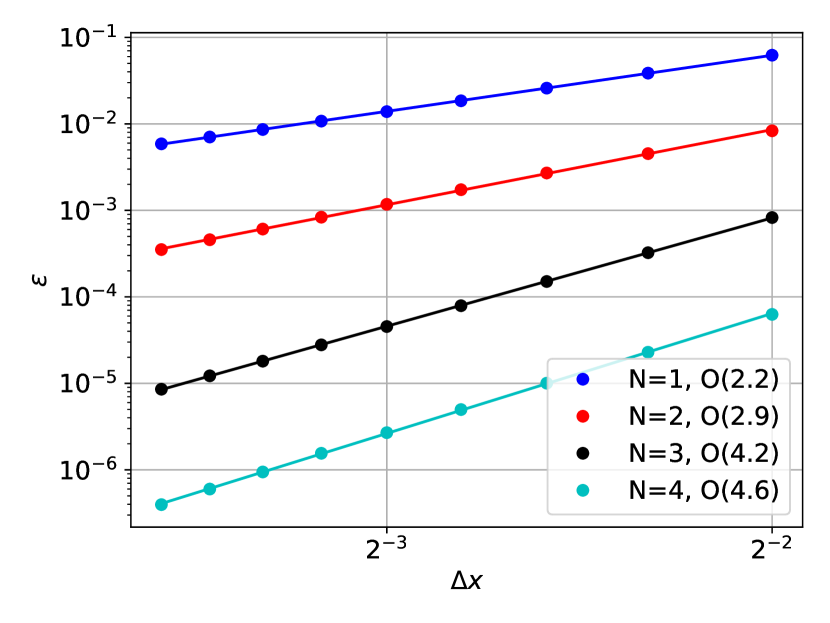
(a) $q$

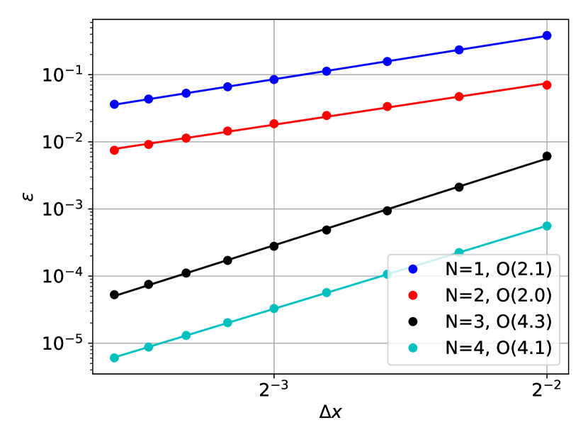
(b) $u_{x}$

Figure 5: L-2 error norms for the linear diffusion equation. Note that $q$ converges at $O(N+1)$, while $\vec{u}$ has an odd-even oscillation between $O(N+1)$ and $O(N)$ convergence rates. $u_{y}$ and $u_{z}$ have near identical plots to $u_{x}$ and are omitted for brevity.

The linear wave equation is defined by

(70) $$\partial_{t}q-v=0$$

(71) $$\partial_{t}\vec{u}-\operatorname{\nabla}v=0$$

(72) $$c=1$$

(73) $$q_{a}(x,y,z,t)=\cos\left(2\pi t\sqrt{3c^{2}}\right)\sin(2\pi x)\sin(2\pi y)\sin(2\pi z)$$

We can recover the traditional wave equation by solving Eq. 70 for $v$ and substituting into Eq. 71 and LABEL:eq:wave3:

$$\partial_{t}\vec{u}-\operatorname{\nabla}\partial_{t}q=0$$

$$\begin{aligned} \partial_{t}(\vec{u}-\operatorname{\nabla}q)&=0&\rightarrow&&\vec{u}&=\operatorname{\nabla}q\end{aligned}$$

$$\partial_{tt}q-\operatorname{\nabla{\cdot}}\left(c^{2}\operatorname{\nabla}q\right)=$$

We choose to not solve the wave equation in this form because of the presence of second order time and spatial derivatives, which our implementation cannot directly handle. Figure 6 demonstrates that all variables present in the simulation converge at the optimal $O(N+1)$ rate. Unlike the diffusion equation the use of central fluxes does not negatively impact convergence rates despite using the same splitting method for the Laplacian operator[5].

(a) $q$

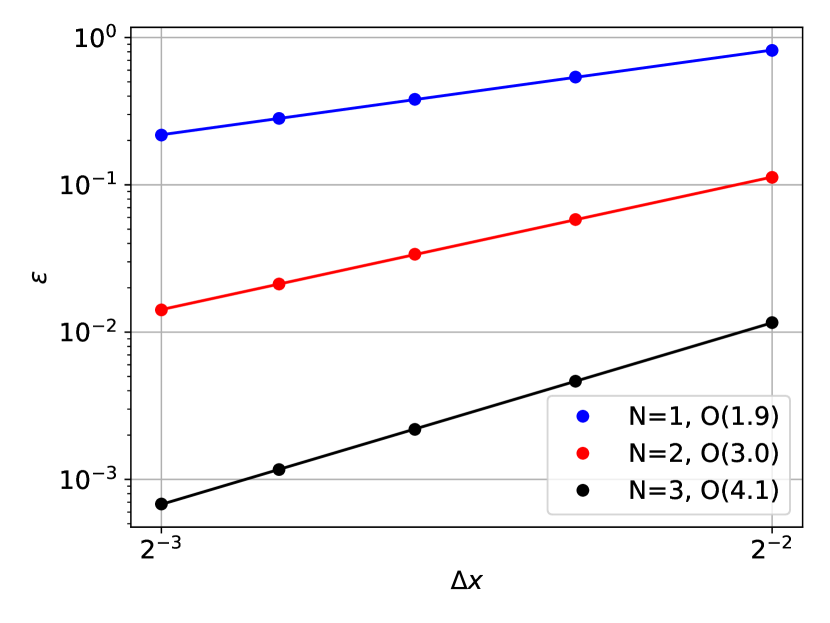
(b) $v$

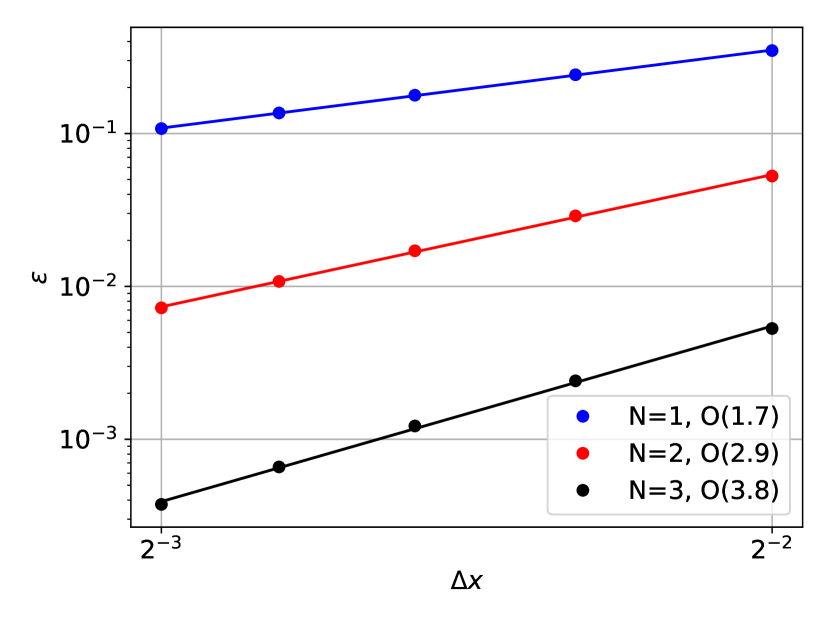
(c) $u_{x}$

Figure 6: L-2 error norms for the linear wave equation. All variables converge at the optimal $O(N+1)$ rate. Plots for $u_{y}$ and $u_{z}$ are nearly identical to $u_{x}$ and omitted.

5 Application of HDG to the two-fluid plasma system

The two-fluid plasma system was used to test the behavior of the HDG code on large coupled systems. A quasi-1D domain of $256\times 1\times 1$ parabolic elements with $x\in[-5,5]$ is initialized with a two-fluid extension of the magnetized Brio-Wu shock tube[23, 16] such that

(74) $$\begin{aligned} \begin{bmatrix}n_{i}\\ U_{i}\\ n_{e}\\ U_{e}\\ B_{x}\\ B_{y}\end{bmatrix}_{\text{left}}&=\begin{bmatrix}1\\ 7.5\times 10^{-5}\\ 1\\ 7.5\times 10^{-5}\\ 7.5\times 10^{-3}\\ 10^{-2}\end{bmatrix}&\begin{bmatrix}n_{i}\\ U_{i}\\ n_{e}\\ U_{e}\\ B_{x}\\ B_{y}\end{bmatrix}_{\text{right}}&=\begin{bmatrix}0.125\\ 7.5\times 10^{-5}\\ 0.125\\ 7.5\times 10^{-6}\\ 7.5\times 10^{-3}\\ -10^{-2}\end{bmatrix}\end{aligned}$$

(75) $$\begin{aligned} \frac{\delta_{p}}{L}&=1&\gamma&=\frac{5}{3}&m_{i}&=1&m_{e}&=\frac{1}{1836}&\frac{c_{0}}{V_{A}}&=c_{h}=c_{p}=1&Z_{i}&=-Z_{e}=10\end{aligned}$$

(76) $$\mu_{c}=\kappa_{c}=Q_{c}=R_{c}=10^{-5}$$

The is simulated from $t\in[0,100]$. Figure 7 shows various plasma properties at the end of the simulation. The plotted fields show similar features to the work of Shumlak and Loverich[23], while being distinct from results produced using standard MHD. Some examples of these differences is the presence of a Whistler wave propagating to the left around $x=1.75$, and the solution producing $T_{i}\neq T_{e}$.

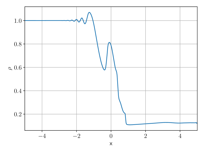
(a) $\rho$

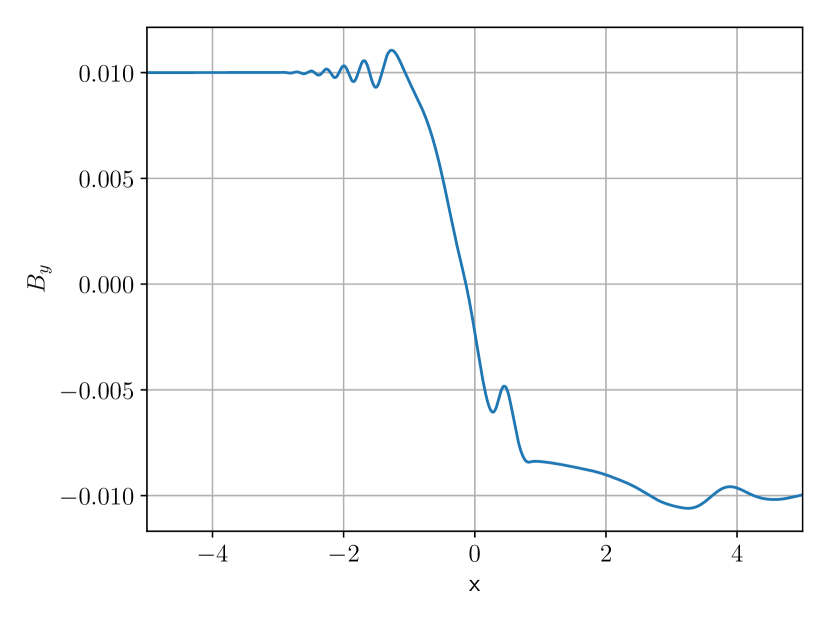
(b) $B_{y}$

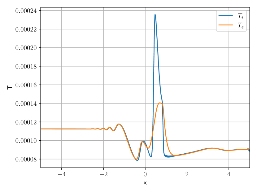
(c) $T$

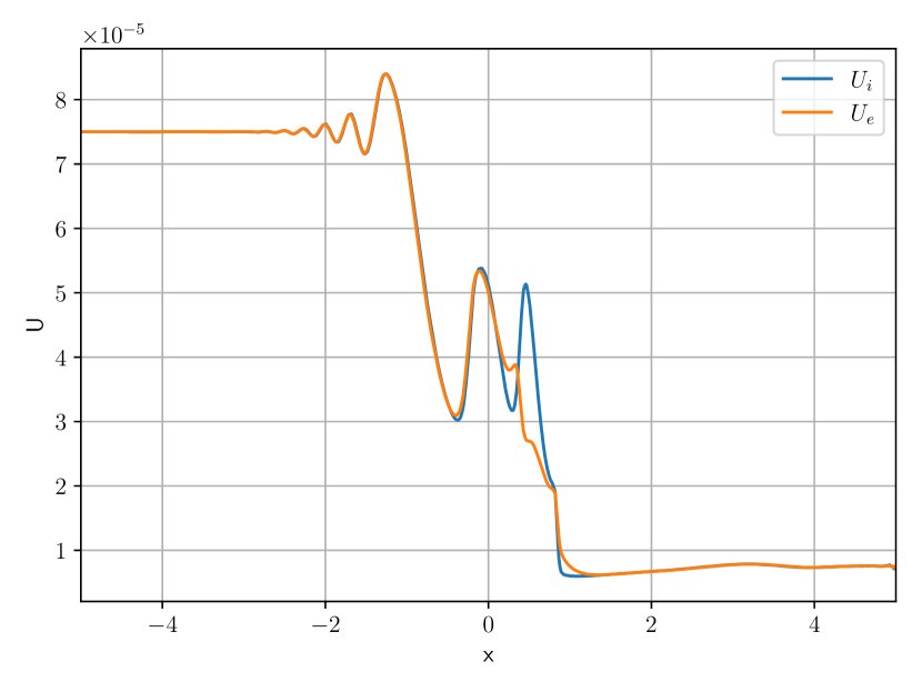
(d) $U$

Figure 7: Two-fluid Brio-Wu shocktube properties at $t=100$. Similar features to those found in Shumlak and Loverich[23] are found, which are notably distinct from the classical MHD results.

To validate the correct propagation speed of various important two-fluid waves, a second simulation with small jumps is initialized to ensure linear behavior. The domain is changed to $1024\times 1\times 1$ linear elements with $x\in[-\pi,\pi]$, and

(77) $$\begin{aligned} \begin{bmatrix}n_{i}\\ U_{i}\\ n_{e}\\ U_{e}\\ B_{x}\\ B_{y}\end{bmatrix}_{\text{left}}&=\begin{bmatrix}10.0005\\ 7.500375\times 10^{-5}\\ 10.0005\\ 7.500375\times 10^{-5}\\ 7.5\times 10^{-2}\\ 5\times 10^{-5}\end{bmatrix}&\begin{bmatrix}n_{i}\\ U_{i}\\ n_{e}\\ U_{e}\\ B_{x}\\ B_{y}\end{bmatrix}_{\text{right}}&=\begin{bmatrix}9.9995\\ 7.499625\times 10^{-5}\\ 9.9995\\ 7.499625\times 10^{-5}\\ 7.5\times 10^{-2}\\ -5\times 10^{-5}\end{bmatrix}\end{aligned}$$

(78) $$\begin{aligned} \frac{\delta_{p}}{L}&=1&\gamma&=\frac{5}{3}&m_{i}&=1&1836m_{e}&=1&\frac{c_{0}}{V_{A}}&=c_{h}=c_{p}=1&Z_{i}&=-Z_{e}=1\end{aligned}$$

(79) $$\mu_{c}=\kappa_{c}=Q_{c}=R_{c}=10^{-5}$$

A mixed 2D spatial/temporal Fourier analysis is then performed on $E_{y}$[23]. This is plotted against the theoretical L and R mode wave propagation speeds, described by the dispersion relation

(80) $$\frac{c_{0}^{2}k^{2}}{V_{A}^{2}\omega^{2}}=1-\frac{\omega_{pe}^{2}}{\omega(\omega\pm\omega_{ce})}$$

(81) $$\begin{aligned} \omega_{pe}&=(\omega_{p}\tau)\sqrt{\frac{n_{e}Z_{e}^{2}}{m_{e}}}&\omega_{ce}&=\frac{L}{\delta_{p}}\frac{|Z_{e}|B}{m_{e}}\end{aligned}$$

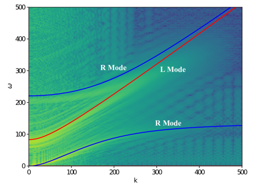
Figure 8: Fourier analysis of $E_{y}$ matches the circularly polarized two-fluid plasma dispersion relation.

Figure 8 demonstrates that the Fourier analysis has three dominant modes corresponding to the three branches of the L and R modes. This test demonstrates the viability of using HDG to solve large-scale coupled plasma differential equations and the validity of the implemented tools to ensure correctness and simplify implementing such solvers.

Figure 9 shows the numerical stability conditions for an equivalent explicit explicit RK4. For analysis purposes the implicit scheme used $\Delta t=6.28\times 10^{-3}$. While an explicit RK4 DG solver can run a $N=0$ basis with this timestep, higher degree basis require a smaller timestep. Define the timestep ratio gain as the implicit timestep $\Delta t$ used divided by the maximum stable explicit timestep. In this case there is a timestep ratio gain of $2.2$ for $N=1$ and $4.4$ for $N=2$ over an explicit RKDG method. The primary reason these ratios are low is that the original test conditions were setup such that it is feasible to run and benchmark an explicit RKDG code. Nevertheless, it is sufficient for demonstrating that the HDG method can continue to operate accurately in a regime where explicit time stepping methods become unstable. In other test problems we have observed stable and accurate runs using timesteps greater than $60$ times larger than allowable for the explicit RK4 DG method.

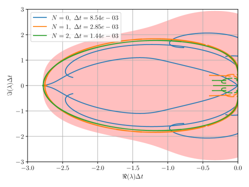
Figure 9: Stability conditions for a two-fluid explicit RK4 DG solver for the above specified conditions. The red highlighted region is the region of absolute stability for RK4 and the curves define the stability eigencurves of the ideal two-fluid system generated using the method from Section 2. Implicit simulations were run with $\Delta t=6.28\times 10^{-3}$ to achieve sufficient temporal resolution for the Fourier dispersion analysis in Fig. 8. A degree 0 basis could be run explicitly with this timestep; however, an explicit solution with a high degree basis is unstable using this timestep.

6 Conclusion

This work increases the viability of using the two-fluid plasma model, which while more physically accurate than single fluid models is numerically stiff[24]. We perform a detailed numerical stability analysis of solving the ideal two-fluid system using classical RKDG. The numerically stiffness of the two-fluid plasma model results from needing to temporally resolve the speed of light, $c_{0}/V_{A}$, and the eigenvalues of the source terms, $\stackrel{{\scriptstyle\leftrightarrow}}{{\boldsymbol{J}}}_{S}$, when bulk plasma motion is dictated by timescales on the order of the ion sound speed. We also demonstrate that hybridizable discontinuous Galerkin enables solving large-scale PDE systems with implicit temporal solvers using a systematic formulation to allow automatic generation of the HDG Schur complement. This systematic process is shown to handle over 40 coupled differential equations and to accurately compute the thousands of analytical non-zero terms of Jacobian, as well as to identify and eliminate variables which analytically vanish. Potential future extensions include implementing bidirectional upwinding numerical fluxes[4] to improve convergence of parabolic/elliptical terms, as well as investigate effective techniques for reducing the time it takes to construct and solve the HDG Schur complement system.

Supplementary Material

A copy of the code can be obtained from https://bitbucket.org/helloworld922/dg.

References

- [1] T. Bui-Thanh, Construction and analysis of hdg methods for linearized shallow water equations, SIAM Journal on Scientific Computing, 38 (2016), pp. A3696–A3719.
- [2] N. Chalmers and L. Krivodonova, A robust cfl condition for the discontinuous galerkin method on triangular meshes, Journal of Computational Physics, 403 (2020), p. 109095, https://doi.org/https://doi.org/10.1016/j.jcp.2019.109095, https://www.sciencedirect.com/science/article/pii/S0021999119308009.
- [3] J. G. Charney, R. FjÖrtoft, and J. V. Neumann, Numerical integration of the barotropic vorticity equation, Tellus, 2 (1950), pp. 237–254, https://doi.org/10.3402/tellusa.v2i4.8607, https://doi.org/10.3402/tellusa.v2i4.8607, https://arxiv.org/abs/https://doi.org/10.3402/tellusa.v2i4.8607.
- [4] B. Cockburn, B. Dong, J. Guzman, M. Restelli, and R. Sacco, A hybridizable discontinuous galerkin method for steady-state convection-diffusion-reaction problems, SIAM Journal on Scientific Computing, 31 (2009), pp. 3827–3846.
- [5] B. Cockburn, N. Nguyen, and J. Peraire, Chapter 8 - hdg methods for hyperbolic problems, in Handbook of Numerical Methods for Hyperbolic Problems, R. Abgrall and C.-W. Shu, eds., vol. 17 of Handbook of Numerical Analysis, Elsevier, 2016, pp. 173–197, https://doi.org/https://doi.org/10.1016/bs.hna.2016.07.001, https://www.sciencedirect.com/science/article/pii/S1570865916300035.
- [6] B. Cockburn and C.-W. Shu, The local discontinuous galerkin method for time-dependent convection-diffusion systems, SIAM Journal on Numerical Analysis, 35 (1997), pp. 2440–2463.
- [7] A. Dedner, F. Kemm, D. Kroner, C.-D. Munz, T. Schnitzer, and M. Wesenberg, Hyperbolic divergence cleaning for the mhd equations, Journal of Computational Physics, 175 (2002), pp. 645–673.
- [8] J. E. Dennis and R. B. Schnabel, Numerical Methods for Unconstrained Optimization and Nonlinear Equations, Society for Industrial and Applied Mathematics, 1996, https://doi.org/10.1137/1.9781611971200, https://epubs.siam.org/doi/abs/10.1137/1.9781611971200, https://arxiv.org/abs/https://epubs.siam.org/doi/pdf/10.1137/1.9781611971200.
- [9] A. H. Glasser and X. Z. Tang, The sel macroscopic modeling code, Computer Physics Communications, (2004), pp. 237–243.
- [10] R. J. Guyan, Reduction of stiffness and mass matrices, AIAA Journal, 3 (1965), pp. 380–380, https://doi.org/10.2514/3.2874, https://doi.org/10.2514/3.2874, https://arxiv.org/abs/https://doi.org/10.2514/3.2874.
- [11] E. Hairer and G. Wanner, Solving Ordinary Differential Equations II, Springer-Verlag, 1980.
- [12] J. S. Hesthaven and T. Warburton, Nodal Discontinuous Galerkin Methods, Springer, 2008.
- [13] R. M. Kirby, S. J. Sherwin, and B. Cockburn, To cg or to hdg: A comparative study, Journal of Scientific Computing, 51 (2012), pp. 183–212.
- [14] F. F.-K. Kuo, Network Analysis and Synthesis, John Wiley & Sons Inc, 2nd ed., 1966.
- [15] J. J. Lee, S. Shannon, an. Bui-Thanh, and J. N. Shadid, Analysis of an hdg method for linearized incompressible resistive mhd equations, SIAM Journal of Numerical Analysis, 57 (2019).
- [16] J. Loverich, A. Hakim, and U. Shumlak, A discontinuous galerkin method for ideal two-fluid plasma equations, Communications in Computational Physics, 9 (2011), pp. 240–268.
- [17] A. Meurer, C. P. Smith, M. Paprocki, O. Čertík, S. B. Kirpichev, M. Rocklin, A. Kumar, S. Ivanov, J. K. Moore, S. Singh, T. Rathnayake, S. Vig, B. E. Granger, R. P. Muller, F. Bonazzi, H. Gupta, S. Vats, F. Johansson, F. Pedregosa, M. J. Curry, A. R. Terrel, v. Roučka, A. Saboo, I. Fernando, S. Kulal, R. Cimrman, and A. Scopatz, Sympy: symbolic computing in python, PeerJ Computer Science, 3 (2017), p. e103, https://doi.org/10.7717/peerj-cs.103, https://doi.org/10.7717/peerj-cs.103.
- [18] C.-D. Munz, P. Ommes, and R. Schneider, A three-dimensional finite-volume solver for the maxwell equations with divergence cleaning on unstructured meshes, Computer Physics Communications, 130 (2000), pp. 83–117.
- [19] N. C. Nguyen and J. Peraire, Hybridizable discontinuous galerkin methods for partial differential equations in continuum mechanics, Journal of Computational Physics, 231 (2012), pp. 5955–5988.
- [20] J. Peraire and P.-O. Persson, The compact discontinuous galerkin (cdg) method for elliptic problems, SIAM Journal on Scientific Computing, 30 (2008), pp. 1806–1824.
- [21] W. Schiesser, The Numerical Method of Lines, Academic Press, 1st ed., 1991.
- [22] U. Shumlak, R. Lilly, N. Reddell, E. Sousa, and B. Srinivasan, Advanced physics calculations using a multi-fluid plasma model, Computer Physics Communications, 182 (2011), pp. 1767–1770, https://doi.org/https://doi.org/10.1016/j.cpc.2010.12.048, https://www.sciencedirect.com/science/article/pii/S001046551100004X. Computer Physics Communications Special Edition for Conference on Computational Physics Trondheim, Norway, June 23-26, 2010.
- [23] U. Shumlak and J. Loverich, Approximate riemann solver for the two-fluid plasma model, Journal of Computational Physics, 187 (2003), pp. 620–638.
- [24] B. Srinivasan and U. Shumlak, Analytical and computational study of the ideal full two-fluid plasma model and asymptotic approximations for Hall-magnetohydrodynamics, Physics of Plasmas, 18 (2011), p. 092113, https://doi.org/10.1063/1.3640811, https://doi.org/10.1063/1.3640811, https://arxiv.org/abs/https://pubs.aip.org/aip/pop/article-pdf/doi/10.1063/1.3640811/13684706/092113_1_online.pdf.
- [25] T. Warburton and T. Hagstrom, Taming the cfl number for discontinuous galerkin methods on structured meshes, SIAM Journal on Numerical Analysis, 46 (2008), pp. 3151–3180, https://doi.org/10.1137/060672601, https://doi.org/10.1137/060672601, https://arxiv.org/abs/https://doi.org/10.1137/060672601.