On a question of Kwakkel and Markovic

Abstract.

A question of F. Kwakkel and V. Markovic on existence of $\mathcal{C}^{1}$-diffeomorphisms of closed surfaces that permute a dense collection of domains with bounded geometry is answered in the negative. In fact, it is proved that for closed surfaces of genus at least one such diffeomorphisms do not exist regardless of whether they have positive or zero topological entropy.

1. Introduction

In [KM10], F. Kwakkel and V. Markovic posed the following question (see below for the definitions):

Question 1.1.

[KM10, Question 1, p. 512] Let $M$ be a closed surface. Do there exist diffeomorphisms $f\in{\rm Diff}^{1}(M)$ with positive entropy that permute a dense collection of domains with bounded geometry?

The authors gave a negative answer under the assumption that $f\in{\rm Diff}^{1+\alpha}(M)$ with $\alpha>0$. In this paper we answer the above question, also in the negative. In fact, we prove that, unless $M$ is the sphere, there are no such diffeomorphisms regardless of whether the entropy is positive or zero.

We recall some definitions from [KM10]. A closed surface $M$ is a smooth, closed, oriented Riemannian 2-manifold, equipped with the canonical metric induced from the standard conformal metric of the universal cover ${\hat{\mathbb{C}}},{\mathbb{C}}$, or ${\mathbb{D}}$, the sphere, the plane, or the unit disk, respectively. Let $S\subset M$ be compact and $\{D_{k}\}_{k\in{\mathbb{Z}}}$ the collection of connected components of the complement of $S$, with the property that ${\rm Int}({\rm Cl}(D_{k}))=D_{k}$, where ${\rm Int}$ and ${\rm Cl}$ stand for the interior and the closure, respectively.

Definition 1.2.

We say that a homeomorphism $f$ of $M$ permutes a dense collection of domains $\{D_{k}\}_{k\in{\mathbb{Z}}}$ if

(1) $f(S)=S$ and ${\rm Cl}(D_{k})\cap{\rm Cl}(D_{k^{\prime}})=\emptyset$ if $k\neq k^{\prime}$,

(2) $f^{n}(D_{k})\cap D_{k}=\emptyset$ for all $k,n\in{\mathbb{Z}},\ n\neq 0$, and

(3) $\bigcup_{k\in{\mathbb{Z}}}D_{k}$ is dense in $M$.

In analogy with Kleinian groups, we refer to the invariant set $S$ in Definition 1.2 above as a limit set of $f$.

Definition 1.3.

A collection of domains $\{D_{k}\}_{k\in{\mathbb{Z}}}$ on a surface $M$ is said to have bounded geometry if ${\rm Cl}(D_{k})$ is contractible in $M$ (i.e., it is contained in an embedded closed topological disk in $M$) and there exists a constant $C\geq 1$ such that for every domain $D_{k}$ in the collection, there are $p_{k}\in D_{k}$ and $0<r_{k}\leq R_{k}$ with

$$B(p_{k},r_{k})\subseteq D_{k}\subseteq B(p_{k},R_{k})\quad{\rm and}\quad R_{k}/r_{k}\leq C.$$

Here, $B(p,r)$ denote an open disk in $M$ centered at $p$ of radius $r>0$.

The main result of this paper is the following theorem.

Theorem 1.4.

If $M$ is a closed surface, other than the sphere, then there does not exist $f\in{\rm Diff}^{1}(M)$ that permutes a dense collection of domains with bounded geometry.

Theorem 1.4 is false in the case when $M={\hat{\mathbb{C}}}$, as can be seen by taking $f(z)=\lambda z,\ \lambda>1$. Indeed, one needs to fill the fundamental annulus $\{z\colon 1\leq|z|<\lambda\}$ with geometric disks and spread them out using the dynamics of $f$.

The paper is organized as follows. In Section 2 we demonstrate existence of an invariant conformal structure on the limit set of a hypothetical $\mathcal{C}^{1}$-diffeomorphism $f$ of $M$ that permutes a dense collection of domains with bounded geometry. In Section 3 we discuss transboundary modulus of curve families and prove existence and uniqueness of extremal distributions for such a modulus. After a short discussion of Nielsen–Thurston classification in Section 4, we proceed by first eliminating in Section 5 the possibility of a hypothetical diffeomorphism $f$ above to be pseudo-Anosov, and then, with the aid of holomorphic quadratic differentials discussed in Section 6, we exclude periodic and reducible diffeomorphisms in the final Section 7.

Acknowledgements. The author thanks Mario Bonk and Misha Lyubich for fruitful conversations, and the Institute for Mathematical Sciences at Stony Brook University for the hospitality.

2. Invariant Conformal Structure

A non-constant orientation preserving homeomorphism $h\colon U\to V$ between open subsets $U$ and $U^{\prime}$ of Riemann surfaces $M$ and $M^{\prime}$, respectively, is called quasiconformal, or $K$-quasiconformal, if the map $h$ is in the Sobolev space $W_{\rm loc}^{1,2}$ and

$$K_{h}(p)=\frac{\max_{|v|=1}D_{p}h(v)}{\min_{|v|=1}D_{p}h(v)}\leq K,\quad{\rm a.e.}\ p\in U.$$

The assumption $h\in W_{\rm loc}^{1,2}$ means that $h$ and the first distributional partial derivatives of $h$ are locally in the Lebesgue space $L^{2}$. The constant $K$ is called a dilatation of $h$. If $K$ can be chosen to be 1 a.e. on a measurable subset $S$ of $U$, the map $h$ is called conformal on $S$.

We will need the following lemma, which we also prove.

Lemma 2.1.

[KM10, Lemma 2.3] Let $M$ be a closed surface and let $f\in{\rm Diff}^{1}(M)$ permute a dense collection of domains $\{D_{k}\}_{k\in{\mathbb{Z}}}$. If the domains in $\{D_{k}\}_{k\in{\mathbb{Z}}}$ have bounded geometry, then $f^{n},\ n\in{\mathbb{Z}}$, have uniformly bounded dilatation on $S=M\setminus\cup_{k\in{\mathbb{Z}}}D_{k}$. I.e., $K_{f^{n}}(p)$ is bounded above by a constant independent of $n\in{\mathbb{Z}}$ and $p\in S$.

Proof.

We assume that $S$ has positive measure, for otherwise there is nothing to prove. Let $\widetilde{M}$ denote the universal cover of $M$ and $\psi\colon\widetilde{M}\to M$ be the projection map. Since $\psi$ is a local isometry, below we make no distinction between $D_{k},\ k\in{\mathbb{Z}}$, that have sufficiently small diameters and their lifts to $\widetilde{M}$ and, whenever convenient, identify the map $f$ with its lift $\tilde{f}$ to $\widetilde{M}$ under the map $\psi$.

Let $n\in{\mathbb{Z}}$ be fixed. Since $S$ is nowhere dense and the closures ${\rm Cl}(D_{k}),\ k\in{\mathbb{Z}}$, are pairwise disjoint, for each $p\in S$ there exists a sequence of complementary components $(D_{k_{i}})_{i\in{\mathbb{N}}}$ of $S$ that accumulate at $p$, i.e.,

$${\rm diam}\,D_{k_{i}}\to 0\quad{\rm and}\quad d_{\rm Hausd}(\overline{D_{k_{i}}},\{p\})\to 0\ {\rm as}\ i\to\infty,$$

where ${\rm diam}$ stands for diameter and $d_{\rm Hausd}$ denotes the Hausdorff distance. Also, since $f$ is $\mathcal{C}^{1}$-differentiable on a compact surface $M$, we have

(1) $$f^{n}(q+x)-f^{n}(q)-D_{q}f^{n}(x)=o(x),\quad x\to 0,$$

where $|o(x)|/|x|\to 0$ as $|x|\to 0$, uniformly in $q$.

The domains $D_{k_{i}},\ i\in{\mathbb{N}}$, having bounded geometry means that there exist $C\geq 1,p_{i}\in D_{k_{i}}$, and $0<r_{i}\leq R_{i},\ i\in{\mathbb{N}}$, with

$$B(p_{i},r_{i})\subseteq D_{k_{i}}\subseteq B(p_{i},R_{i}),\quad{\rm and}\quad{R_{i}}/{r_{i}}\leq C.$$

Thus, by possibly passing to a subsequence, we may assume that the Hausdorff limit of the rescaled domains

$$\left((D_{k_{i}}-p_{i})/r_{i}\right)_{i\in{\mathbb{N}}}$$

is a closed set $\Omega$ such that

(2) $$\overline{B(0,1)}\subseteq\Omega\subseteq\overline{B(0,C)}.$$

Let $D_{k_{i}}^{\prime},\ i\in{\mathbb{N}}$, denote the image of $D_{k_{i}},\ i\in{\mathbb{N}}$, under the map $f^{n}$. Because $f^{n}$ is in ${\rm Diff}^{1}(M)$, and hence is locally bi-Lipschitz, after possibly passing to yet a further subsequence, we may assume that the sequence

$$\left((D_{k_{i}}^{\prime}-f^{n}(p_{i}))/r_{i}\right)_{i\in{\mathbb{N}}}$$

Hausdorff converges to a closed set $\Omega^{\prime}$. Similar to (2), we know that there exists $p^{\prime}\in\Omega^{\prime}$ and $r^{\prime}>0$ such that

(3) $$\overline{B(p^{\prime},r^{\prime})}\subseteq\Omega^{\prime}\subseteq\overline{B(p^{\prime},Cr^{\prime})},$$

where the constant $C\geq 1$ is the same as above. Since Equation (1) is uniform in $q$, in particular it holds for $q=p_{i},\ q+x\in D_{k_{i}},\ i\in{\mathbb{N}}$, one concludes that

(4) $$\Omega^{\prime}=D_{p}f^{n}(\Omega).$$

Combining (2), (3), and (4), and using the fact that the constant $C$ does not depend on $p\in S$ or $n\in{\mathbb{Z}}$, we conclude that the maps $f^{n},\ n\in{\mathbb{Z}}$, has uniformly bounded dilatation on $S$, as claimed. ∎

In the proof of Theorem 1.4 we use a modification, Proposition 2.2 below, of a result by P. Tukia [Tu80] (see also [Su78]). A Beltrami form on a measurable subset $S$ of a Riemann surface $M$ is a measurable $(-1,1)$-form on $S$ given in a local chart by $\mu=\mu(z)d\bar{z}/dz$, where we assume that $\|\mu\|_{\infty}<1$; see, e.g., [BF14] for background on Beltrami forms. If $h\colon U\to U^{\prime}$ is a quasiconformal map between open subsets $U$ and $U^{\prime}$ of $M$ and $M^{\prime}$, respectively, and $\mu$ is a Beltrami form on $U^{\prime}$, the pullback of $\mu$ under $h$ is the Beltrami form given in local charts by

$$h^{*}(\mu)=\left(\frac{h_{\bar{z}}+\mu(h)\overline{h_{z}}}{h_{z}+\mu(h)\overline{h_{\bar{z}}}}\right)\frac{d\bar{z}}{dz}.$$

The pullback of the 0 Beltrami form is denoted by $\mu_{h}$. We say that a Beltrami form $\mu$ on $S$ is invariant under $h$ if $S$ is invariant under $h$, i.e., $S\subseteq U=U^{\prime},\ h(S)=S$ up to a measure zero set, and $\mu=h^{*}(\mu).$ In particular, 0 Beltrami form is invariant under $h$ if and only if $h$ is conformal on $S$.

Proposition 2.2.

Let $M$ be a Riemann surface and $S\subseteq M$ be a measurable subset. Let $H$ be a countable group of quasiconformal maps $h$ of $M$ that leave $S$ invariant and that have uniformly bounded dilatation on $S$. Then there exists a Beltrami form $\mu$ on $S$ that is invariant under each map $h\in H$.

Proof.

As in Lemma 2.1, we may assume that $S$ has positive measure, for otherwise there is nothing to prove.

For arbitrary quasiconformal maps $f,g$, expressing $\mu_{g\circ f}$ in terms of $\mu_{g}$ and $\mu_{f}$, we have

(5) $$\mu_{g\circ f}=f^{*}(\mu_{g})=T_{f}(\mu_{g}(f)),$$

where

$$T_{f}(w)=\frac{\mu_{f}+\frac{\overline{f_{z}}}{f_{z}}w}{1+\overline{\mu_{f}}\frac{\overline{f_{z}}}{f_{z}}w}$$

is an isometry of the disk model hyperbolic plane ${\mathbb{D}}$ for a.e.  $z$.

We consider

$$B(z)=\{\mu_{h}(z)\colon\ h\in H\},$$

a subset of ${\mathbb{D}}$ defined for a.e. $z\in S$ up to a rotation which depends on a local chart. Since $H$ is a group, Equation (5) gives

(6) $$T_{h}(B(h(z))) =\left\{T_{h}(\mu_{h^{\prime}}(h(z)))\colon h^{\prime}\in H\right\}$$

$$=\left\{\mu_{h^{\prime}\circ h}(z)\colon h^{\prime}\in H\right\}=B(z),$$

for each $h\in H$, a.e. $z\in S$, and an appropriate choice of local charts $z$ and $h(z)$. If $B$ is a non-empty bounded subset of ${\mathbb{D}}$, we define by $P(B)$ to be the center of the smallest closed hyperbolic disk that contains $B$. Elementary hyperbolic geometry shows that $P(B)$ is well defined. Moreover, $P$ satisfies (see [Tu80] for details):

1) if $B$ is bounded above by $\delta$ in the hyperbolic metric of ${\mathbb{D}}$, then $P(B)$ is at most hyperbolic distance $\delta$ from the origin in ${\mathbb{D}}$;

2) the map $P$ commutes with each hyperbolic isometry of ${\mathbb{D}}$, i.e.,

$$P(T(B))=T(P(B))$$

for any hyperbolic isometry $T$ of ${\mathbb{D}}$ and arbitrary non-empty bounded subset $B$ of ${\mathbb{D}}$.

We now define, for a.e. $z\in S$,

$$\mu(z)=P(B(z)).$$

This definition, even though dependent on local charts, gives rise to a global Beltrami form $\mu$ on $M$ because $P$ commutes with rotations. The assumption that the elements of $H$ are $K$-quasiconformal on $S$ with the same constant $K$ and property 1) above give that $\mu$ is an essentially bounded Beltrami form. Equation (6) combined with the commutative property 2) give, in appropriate local charts,

$$\mu(z)=P(B(z))=P(T_{h}(B(h(z))))=T_{h}(P(B(h(z))))=T_{h}(\mu(h(z))),$$

for each $h\in H$ and a.e. $z$ in $S$. By (5), this is equivalent to

$$\mu=h^{*}(\mu),$$

on $S$ for each $h\in H$, i.e., $\mu$ is invariant under each $h\in H$. ∎

An alternative proof of Proposition 2.2 uses the barycenter of the convex hull to define $\mu$ rather than the center of the smallest hyperbolic disk as above. This approach was used in [Su78].

An application of the Measurable Riemann Mapping Theorem [BF14, Theorem 1.27] gives that for the Beltrami form $\mu$ from Proposition 2.2, extended by 0 outside $S$, there exists a Riemann surface $M^{\prime}$ and a quasiconformal homeomorphism $\phi\colon M\to M^{\prime}$ such that $\mu=\mu_{\phi}$. Since conformality of a quasiconformal map $h$ of $M$ on an invariant measurable subset $S$ is equivalent to the 0 Beltrami form being invariant under $h$, we get the following corollary to Proposition 2.2.

Corollary 2.3.

Let $M$ be a Riemann surface and $S\subseteq M$ be a measurable subset. Let $H$ be a countable group of quasiconformal maps $h$ of $M$ that leave $S$ invariant and that have uniformly bounded dilatation on $S$. Then there exists a quasiconformmal map $\phi\colon M\to M^{\prime}$ of $M$ onto another Riemann surface $M^{\prime}$ such that the conjugate family $H^{\prime}=\{\phi\circ h\circ\phi^{-1}\colon h\in H\}$ consists of quasiconformal maps of $M^{\prime}$ that leave $S^{\prime}=\phi(S)$ invariant and are conformal on it.

3. Transboundary modulus

The following notion of modulus is inspired by O. Schramm’s transboundary extremal length, introduced in [Sch95]. An adaptation in the setting of Sierpiński carpets has been used extensively, notably in [Bo11, BM13].

Let $M$ be a closed surface and $\sigma$ the area measure on $M$. By a mass density we mean a non-negative measurable function $\rho$ on $M$. If $\Gamma$ is a curve family in $M$, a mass density $\rho$ is called admissible for $\Gamma$ if

$$\int_{\gamma}\rho\,ds\geq 1,\quad{\rm for\ all}\ \gamma\in\Gamma,$$

where $ds$ denotes the arc-length element. The $2$-modulus of $\Gamma$ is defined as

$${\rm mod}_{2}(\Gamma)=\inf\left\{\int_{M}\rho^{2}d\sigma\right\},$$

where the infimum is taken over all $\rho$ that are admissible for $\Gamma$.

Let $S\subset M$ be a compact set and $M\setminus S=\cup_{k\in{\mathbb{Z}}}D_{k}$, where $\{D_{k}\}_{k\in{\mathbb{Z}}}$ is a non-empty collection of disjoint complementary components of $S$. If $\Gamma$ is a family of curves in $M$, then we define the transboundary modulus of $\Gamma$ with respect to $S$, denoted by ${\rm mod}_{S}(\Gamma)$, as follows. Let $\rho$ be a mass distribution for $S$, i.e., a function $\rho\colon S\cup\{D_{k}\colon k\in{\mathbb{Z}}\}\to[0,+\infty]$, where the restriction $\rho|_{S}$ is a measurable non-negative function, and $\rho(D_{k}),\ k\in{\mathbb{Z}}$, is a non-negative number for each $k\in{\mathbb{Z}}$. We refer to $\rho|_{S}$ as the continuous part of a mass distribution $\rho$ and to $\{\rho(D_{k})\}_{k\in{\mathbb{Z}}}$ as the discrete part. A mass distribution $\rho$ is admissible for $\Gamma$ if there exists $\Gamma_{0}\subseteq\Gamma,\ {\rm mod}_{2}(\Gamma_{0})=0$, called an exceptional curve family, such that

(7) $$\int_{\gamma\cap S}\rho\,ds+\sum_{k\colon\gamma\cap D_{k}\neq\emptyset}\rho(D_{k})\geq 1,$$

for each $\gamma\in\Gamma\setminus\Gamma_{0}$. (Below it should be clear from context which notion of admissibility, i.e., for 2-modulus or for transboundary modulus, is used.) We set

(8) $${\rm mod}_{S}(\Gamma)=\inf\left\{{\rm mass}(\rho)\right\},$$

where the infimum is taken over all mass distributions $\rho$ that are admissible for $\Gamma$, and

(9) $${\rm mass}(\rho)=\int_{S}\rho^{2}d\sigma+\sum_{k\in{\mathbb{Z}}}\rho(D_{k})^{2}$$

is the total mass of $\rho$. If the set $S$ has measure zero, then we ignore the continuous part of distribution $\rho$ in (7) and (9). Excluding an exceptional curve family $\Gamma_{0}$ ensures that in many interesting cases and for some relevant curve families $\Gamma$ an admissible mass distribution exists and $0<{\rm mod}_{S}(\Gamma)<\infty$.

We think of a mass distribution $\rho$ as an element of the direct sum Banach space $L^{2}\oplus l^{2}$, where $L^{2}=L^{2}(S)$, and $l^{2}$ consists of all sequences $(\rho_{k})_{k\in{\mathbb{Z}}}$ with $\sum_{k}\rho_{k}^{2}<\infty$. The norm of $\rho\in L^{2}\oplus l^{2}$ is given by $\|\rho\|_{L^{2}\oplus l^{2}}=\left(\|\rho\|_{L^{2}}^{2}+\|\rho\|_{l^{2}}^{2}\right)^{1/2}$, where

$$\|\rho\|_{L^{2}}=\left(\int_{S}\rho^{2}d\sigma\right)^{1/2},\quad\|\rho\|_{l^{2}}=\left(\sum_{k\in{\mathbb{Z}}}\rho_{k}^{2}\right)^{1/2}.$$

Transboundary modulus has some familiar properties of the $2$-modulus, with almost identical proofs, e.g., quasi-invariance under quasiconformal maps, monotonicity, and subadditivity. Quasi-invariance is the property that if $h\colon M\to M^{\prime}$ is a quasiconformal map between two Riemann surfaces, then there exists a constant $C\geq 1$ such that for every curve family $\Gamma$ in $M$ one has

$$\frac{1}{C}\,{\rm mod}_{S}(\Gamma)\leq{\rm mod}_{S^{\prime}}(\Gamma^{\prime})\leq C\,{\rm mod}_{S}(\Gamma),$$

where $S^{\prime}=h(S)$ and $\Gamma^{\prime}=h(\Gamma)=\{h(\gamma)\colon\gamma\in\Gamma\}$. If $h$ is conformal, the modulus is invariant, i.e., $C=1$. Monotonicity means that if $\Gamma^{\prime}\subseteq\Gamma$, then

$${\rm mod}_{S}(\Gamma^{\prime})\leq{\rm mod}_{S}(\Gamma).$$

Subadditivity says that if $\Gamma=\cup_{i\in{\mathbb{N}}}\Gamma_{i}$, then

$${\rm mod}_{S}(\Gamma)\leq\sum_{i\in{\mathbb{N}}}{\rm mod}(\Gamma_{i}).$$

The following proposition is the main result of this section.

Proposition 3.1.

If $\Gamma$ is a curve family with ${\rm mod}_{S}(\Gamma)<\infty$, and if $\{D_{k}\}_{k\in{\mathbb{Z}}}$ have bounded geometry, then an extremal distribution $\rho$, i.e., an admissible distribution for which the infimum in the definition (8) is achieved, exists and is unique as an element of $L^{2}\oplus l^{2}$.

The proof of this proposition below mimics that of [BM13, Proposition 2.4] and requires auxiliary results.

3.1. Auxiliary lemmas

As above, let $M$ be a closed surface and $\sigma$ its area measure. To prove Proposition 3.1 we need Lemma 3.3 below (cf. [BM13, Lemma 2.3]), which, in turn, requires the following lemma.

Lemma 3.2.

[Bo88], [BM13, Lemma 2.2] Let $\{B_{k}\}_{k\in I}$ be a finite or countable collection of disjoint geometric balls in a closed surface $M$. Further, let $\{a_{k}\}_{k\in I}$ be non-negative numbers. Then, for each $\lambda\geq 1$ there exists $C\geq 0$ such that

(10) $$\left\|\sum_{k\in I}a_{k}\chi_{\lambda B_{k}}\right\|_{L^{2}}\leq C\left\|\sum_{k\in I}a_{k}\chi_{B_{k}}\right\|_{L^{2}}.$$

Lemma 3.3.

Let $M$ be a closed surface and $S\subset M$ be a compact subset such that $S=M\setminus\cup_{k\in{\mathbb{Z}}}D_{k}$, where domains $D_{k},\ k\in{\mathbb{Z}}$, have bounded geometry. If $\Gamma$ is a curve family in $M$, then ${\rm mod}_{S}(\Gamma)=0$ implies ${\rm mod}_{2}(\Gamma)=0$.

Proof.

Since $\Gamma$ cannot contain constant curves, we have

$$\Gamma=\cup_{i\in{\mathbb{N}}}\Gamma_{i},\quad{\rm where}\quad\Gamma_{i}=\{\gamma\in\Gamma:\ {\rm diam}(\gamma)\geq 1/i\}.$$

From subadditivity of ${\rm mod}_{2}$ it follows that it is enough to show that ${\rm mod}_{2}(\Gamma_{i})=0$ for each $i\in{\mathbb{N}}$. We fix $i\in{\mathbb{N}}$. Monotonicity of ${\rm mod}_{S}$ gives that ${\rm mod}_{S}(\Gamma_{i})=0$. Thus, for each $l\in{\mathbb{N}}$, there exists a mass distribution $\rho_{i,l}$ with ${\rm mass}(\rho_{i,l})<1/2^{l}$, and an exceptional curve family $\Gamma_{i,l}$ such that

$$\int_{\gamma\cap S}\rho_{i,l}\,ds+\sum_{k\colon\gamma\cap D_{k}\neq\emptyset}\rho_{i,l}(D_{k})\geq 1,$$

for all $\gamma\in\Gamma_{i}\setminus\Gamma_{i,l}$.

Let $\rho_{i}=\sum_{l\in{\mathbb{N}}}\rho_{i,l}$ and $\Gamma_{i,\infty}=\cup_{l\in{\mathbb{N}}}\Gamma_{i,l}$. Then, ${\rm mass}(\rho_{i})<\infty$ and subadditivity of ${\rm mod}_{2}$ gives ${\rm mod}_{2}(\Gamma_{i,\infty})=0$. Moreover,

(11) $$\int_{\gamma\cap S}\rho_{i}\,ds+\sum_{k\colon\gamma\cap D_{k}\neq\emptyset}\rho_{i}(D_{k})=\infty$$

for all $\gamma\in\Gamma_{i}\setminus\Gamma_{i,\infty}$.

Recall, the bounded geometry assumption is, for each $k\in{\mathbb{Z}}$, the existence of disks $B(p_{k},r_{k}),B(p_{k},R_{k})$ such that

$$B(p_{k},r_{k})\subseteq D_{k}\subseteq B(p_{k},R_{k}),\quad{\rm with}\quad{R_{k}}/{r_{k}}\leq C.$$

Now we define a mass density $\rho$ on $M$ by the formula

$$\rho=\rho_{i}+\sum_{k\in{\mathbb{Z}}}\frac{\rho_{i}(D_{k})}{R_{k}}\chi_{B(p_{k},2R_{k})},$$

where the first summand is extended to the complement of $S$ as 0. We first claim that for each $\gamma\in\Gamma_{i}\setminus\Gamma_{i,\infty}$ one has

(12) $$\int_{\gamma}\rho\,ds=\infty.$$

Indeed, for all but finitely many $k$, since ${\rm diam}(\gamma)\geq 1/i$, if $\gamma$ intersects $D_{k}\subseteq B(p_{k},R_{k})$, it intersects both complementary components of $B(p_{k},2R_{k})\setminus B(p_{k},R_{k})$. This implies

$$\int_{\gamma}\chi_{B(p_{k},2R_{k})}ds\geq R_{k},$$

and the claim follows from Equation (11). Next, from Lemma 3.2 we conclude

(13) $$\int_{M}\rho^{2}d\sigma \leq 2\left(\int_{S}\rho_{i}^{2}d\sigma+C^{2}\sum_{k\in{\mathbb{Z}}}\frac{\rho_{i}(D_{k})^{2}}{R_{k}^{2}}\sigma\left(B(p_{k},r_{k})\right)\right)$$

$$\leq C(M)\cdot{\rm mass}(\rho_{i})<\infty,$$

where $C(M)$ is a constant that depends on the manifold $M$. Then, (12) and (13) imply ${\rm mod}_{2}(\Gamma_{i}\setminus\Gamma_{i,\infty})=0$. Hence,

$${\rm mod}_{2}(\Gamma_{i})\leq{\rm mod}_{2}(\Gamma_{i,\infty})+{\rm mod}_{2}(\Gamma_{i}\setminus\Gamma_{i,\infty})=0.$$

∎

3.2. Proof of Proposition 3.1

Let $(\rho_{i})_{i\in{\mathbb{N}}}$ be a minimizing sequence of admissible mass distributions for $\Gamma$, i.e.,

$${\rm mass}(\rho_{i})\to{\rm mod}_{S}(\Gamma),\quad i\to\infty.$$

The condition ${\rm mod}_{S}(\Gamma)<\infty$ allows us to assume that ${\rm mass}(\rho_{i})\leq C$ for some constant $C>0$ and all $i\in{\mathbb{N}}$. By the Banach–Alaoglu Theorem, there exists a subsequence of $(\rho_{i})_{i\in{\mathbb{N}}}$ that weakly converges to a mass distribution $\rho\in L^{2}\oplus l^{2}$. In particular, we may assume that the limits

$$\rho(D_{k})=\lim_{i\to\infty}\rho_{i}(D_{k})$$

exist for all $k\in{\mathbb{Z}}$. We claim that the mass distribution $\rho$ is extremal.

One inequality, namely ${\rm mass}(\rho)\leq{\rm mod}_{S}(\Gamma)$ follows from the weak lower semicontinuity of norms. To show the reverse inequality, one needs to demonstrate that $\rho$ is admissible for $\Gamma$. Since the sequence $(\rho_{i})_{i\in{\mathbb{N}}}$ converges weakly to $\rho\in L^{2}\oplus l^{2}$, Mazur’s Lemma [Yo80, Th. 2, p. 120] gives that there is a sequence $(\tilde{\rho}_{K})_{K\in{\mathbb{N}}}$ of convex combinations,

$$\tilde{\rho}_{K}=\sum_{i=1}^{K}\lambda_{K,i}\rho_{i},$$

that strongly converges to $\rho$ in $L^{2}\oplus l^{2}$. Therefore, $(\tilde{\rho}_{K})_{K\in{\mathbb{N}}}$ is also a minimizing sequence for ${\rm mod}_{S}(\Gamma)$. Moreover, each $\tilde{\rho}_{K},\ K\in{\mathbb{N}}$, is trivially admissible for $\Gamma$. An exceptional curve family $\widetilde{\Gamma}_{K}$ for $\tilde{\rho}_{K}$ is the union of exceptional curve families for $\rho_{i},\ i=1,2,\dots,K$. By possibly passing to a subsequence, we may assume that

$$\left\|\tilde{\rho}_{K}-\rho\right\|_{L^{2}\oplus l^{2}}\leq\frac{1}{2^{K}},\quad K\in{\mathbb{N}}.$$

Let

$$\Gamma_{K}^{\prime}=\left\{\gamma\in\Gamma\colon\int_{\gamma\cap S}|\tilde{\rho}_{K}-\rho|\,ds+\sum_{k\colon\gamma\cap D_{k}\neq\emptyset}|\tilde{\rho}_{K}(D_{k})-\rho(D_{k})|\geq\frac{1}{K}\right\},$$

and

$$\Gamma^{\prime}=\cap_{i\in{\mathbb{N}}}\cup_{K\geq i}\Gamma^{\prime}_{K}.$$

From this definition we have that if $\gamma\in\Gamma\setminus\Gamma^{\prime}$, then

$$\limsup_{K\to\infty}\left(\int_{\gamma\cap S}|\tilde{\rho}_{K}-\rho|\,ds+\sum_{k\colon\gamma\cap D_{k}\neq\emptyset}|\tilde{\rho}_{K}(D_{k})-\rho(D_{k})|\right)=0.$$

The mass distributions

$$\rho_{i}^{\prime}=\sum_{K=i}^{\infty}K|\tilde{\rho}_{K}-\rho|,\quad i\in{\mathbb{N}},$$

are admissible for $\Gamma^{\prime}$, and since $\left\|\tilde{\rho}_{K}-\rho\right\|_{L^{2}\oplus l^{2}}\leq{1}/{2^{K}}$, we have that ${\rm mass}(\rho_{i}^{\prime})\to 0,\ i\to\infty$. Thus, ${\rm mod}_{S}(\Gamma^{\prime})=0$. Lemma 3.3 then gives ${\rm mod}_{2}(\Gamma^{\prime})=0$. We conclude that $\Gamma_{\infty}=\Gamma^{\prime}\cup\left(\cup_{K\in{\mathbb{N}}}\widetilde{\Gamma}_{K}\right)$ is an exceptional family for $\rho$. Indeed, subadditivity gives ${\rm mod}_{2}(\Gamma_{\infty})=0$, and for each $\gamma\in\Gamma\setminus\Gamma_{\infty}$, since each $\tilde{\rho}_{K}$ is admissible,

$$\int_{\gamma\cap S}\rho\,ds+\sum_{k\colon\gamma\cap D_{k}\neq\emptyset}\rho(D_{k})$$

$$\geq 1-\limsup_{K\to\infty}\left(\int_{\gamma\cap S}|\tilde{\rho}_{K}-\rho|\,ds+\sum_{k\colon\gamma\cap D_{k}\neq\emptyset}|\tilde{\rho}_{K}(D_{k})-\rho(D_{k})|\right)=1.$$

This completes the proof of existence of an extremal mass distribution for ${\rm mod}_{S}(\Gamma)$.

A simple convexity argument implies that an extremal distribution $\rho$ is also unique. Indeed, if there exists another, different, extremal mass distribution $\rho^{\prime}$, then the average $(\rho+\rho^{\prime})/2$ is also admissible for $\Gamma$. The strict convexity of $L^{2}\oplus l^{2}$, now gives that the average has a strictly smaller total mass, a contradiction. ∎

To finish this section, we prove the following conformal invariance lemma that makes transboundary modulus particularly useful. Let $f\colon M\to M^{\prime}$ be a homeomorphism between Riemann surfaces that takes a compact set $S=M\setminus\cup_{k\in{\mathbb{Z}}}D_{k}$ onto $S^{\prime}=M^{\prime}\setminus\cup_{k\in{\mathbb{Z}}}D_{k}^{\prime}$. Assume that $f$ is conformal on $S$, and $\rho$ is a mass distribution for $S^{\prime}$. We define the pullback distribution $f^{*}(\rho)$ to be $\rho(f)|f^{\prime}|$ on $S$ and $f^{*}(\rho)(D_{k})=\rho(f(D_{k})),\ k\in{\mathbb{Z}}$, where $f^{\prime}$ is the derivative of $f$.

Lemma 3.4.

Let $f\colon M\to M^{\prime}$ be quasiconformal homeomorphism that is conformal a.e. on $S=M\setminus\cup_{k\in{\mathbb{Z}}}D_{k}$. Let $\Gamma$ be an arbitrary curve family in $M$. If $\rho$ is the extremal mass distribution for $f(\Gamma)=\{f(\gamma)\colon\gamma\in\Gamma\}$, then the pullback distribution $f^{*}(\rho)$ is the extremal mass distribution for $\Gamma$. Moreover,

$${\rm mod}_{f(S)}(f(\Gamma))={\rm mod}_{S}(\Gamma).$$

Proof.

Let $\Gamma_{0}\subseteq f(\Gamma)$ be an exceptional curve family for $\rho$, and let $\Gamma_{0}^{\prime}=f^{-1}(\Gamma_{0})$ be the preimage family. Then, since $f$ is quasiconformal, the geometric definition of quasiconformality gives ${\rm mod}_{2}(\Gamma_{0}^{\prime})=0$; see [He01]. In addition, let $\Gamma_{0}^{\prime\prime}$ be the family of curves on which $f$ is not absolutely continuous. Again, since $f$ is quasiconformal, we have ${\rm mod}_{2}(\Gamma_{0}^{\prime\prime})=0$, and thus ${\rm mod}_{2}(\Gamma_{0}^{\prime}\cup\Gamma_{0}^{\prime\prime})=0$. If $\gamma\in\Gamma\setminus(\Gamma_{0}^{\prime}\cup\Gamma_{0}^{\prime\prime})$, then, in particular, $f(\gamma)\in\Gamma\setminus\Gamma_{0}$, and hence

$$\int_{\gamma\cap S}\rho(f)|f^{\prime}|\,ds+\sum_{k\colon\gamma\cap D_{k}\neq\emptyset}\rho(f(D_{k}))$$

$$=\int_{f(\gamma)\cap S}\rho\,ds+\sum_{k\colon f(\gamma)\cap D_{k}\neq\emptyset}\rho(D_{k})\geq 1,$$

i.e., the pullback mass distribution $f^{*}(\rho)$ is admissible for $\Gamma$. The total mass of $f^{*}(\rho)$ is

$$\int_{S}\rho(f)^{2}|f^{\prime}|^{2}d\sigma+\sum_{k\in{\mathbb{Z}}}\rho(f(D_{k}))^{2}=\int_{S}\rho^{2}d\sigma+\sum_{k\in{\mathbb{Z}}}\rho(D_{k})^{2},$$

i.e., it is equal to ${\rm mass}(\rho)$. Therefore,

$${\rm mod}_{S}(\Gamma)\leq{\rm mod}_{S}(f(\Gamma)).$$

The converse inequality, and indeed the full lemma, follow from the facts that the inverse of a quasiconformal map is quasiconformal, and the inverse of a conformal map is conformal. ∎

4. Nielsen–Thurston Classification

Recall that the mapping class group of a closed surface $M$, denoted ${\rm Mod}(M)$, is the group of isotopy classes of orientation preserving homeomorphisms ${\rm Homeo}^{+}(M)$. Equivalently,

$${\rm Mod}(S)={\rm Homeo}^{+}(M)/{\rm Homeo}_{0}(M),$$

where ${\rm Homeo}_{0}(M)$ denotes the connected component of the identity in ${\rm Homeo}^{+}(M)$. There are several equivalent variations of the definition of the mapping class group, for example, where homeomorphisms are replaced by diffeomorphisms or isotopy classes replaced by homotopy classes. For this and other facts and properties of mapping class groups one can consult [FM12].

Theorem 4.1.

[FM12, Theorems 13.1, 13.2] If $M$ is a closed surface, each $f\in{\rm Mod}(M)$ is either periodic, or reducible, or pseudo-Anosov.

Recall, an element $f\in{\rm Mod}(M)$ is called periodic if there is $n\in{\mathbb{N}}$ such that $f^{n}$ is isotopic to the identity. An element $f\in{\rm Mod}(M)$ is called reducible if there is a non-empty set $\{[c_{1}],\dots,[c_{k}]\}$ of isotopy classes of essential simple closed curves in $M$ such that $i([c_{i}],[c_{j}])=0,\ i\neq j$, and $[f(c_{i})]=[c_{i}]$ for all $i=1,2\dots,k$. Here, $[c]$ denotes the homotopy class of a simple closed curve $c$, and $i([a],[b])$ denotes the geometric intersection number, i.e., the minimal number of intersection points between a representative curve in the homotopy class $[a]$ and a representative curve in the class $[b]$. Finally, an element $f\in{\rm Mod}(M)$ is called pseudo-Anosov if there exists a pair of transverse measured foliations $(\mathcal{F}^{s},\mu_{s})$ and $(\mathcal{F}^{u},\mu_{u})$ on $M$, the former is called stable and the latter unstable, a stretch factor$\lambda>1$, and a representative pseudo-Anosov homeomorphism $\phi$, i.e.,

$$\phi\cdot(\mathcal{F}^{s},\mu_{s})=(\mathcal{F}^{s},\lambda^{-1}\mu_{s})\quad{\rm and}\quad\phi\cdot(\mathcal{F}^{u},\mu_{u})=(\mathcal{F}^{u},\lambda\mu_{u}).$$

This definition includes Anosov classes on 2-torus ${\mathbb{T}}^{2}$. The difference between Anosov and pseudo-Anosov classes is that transverse measured foliations of the latter may have singularities.

5. Pseudo-Anosov diffeomorphisms

Let $M$ be a closed (oriented) surface of genus at least 1. As above, we assume that $M$ is equipped with the canonical metric induced from the standard conformal metric of the universal cover ${\mathbb{C}}$ or ${\mathbb{D}}$. Let $\gamma$ be a homotopically non-trivial simple closed curve in $M$ and $D$ be a contractible domain in $M$. We say that there are $N$ essential intersections of $\gamma$ with $D$ if $\gamma\setminus{\rm Cl}(D)$ has $N$ open arcs $\alpha$, and only these arcs, such that $\alpha\cup{\rm Cl}(D)$ is not contractible in $M$. Slightly abusing the terminology, we call the $N$ complementary closed arcs $\beta$ of $\gamma$ to the open arcs $\alpha$ essential intersections of $\gamma$ with $D$. Since any homeomorphism $f$ of $M$ preserves the property of a curve or set to be contractible, for any homotopically non-trivial curve $\gamma$ in $M$ and any contractible domain $D$, the curve $f(\gamma)$ has $N$ essential intersections with $f(D)$ if and only if $\gamma$ has $N$ essential intersections with $D$.

Let $\gamma_{0}$ be a simple closed geodesic in $M$. For a small $\epsilon_{0}>0$, let $\gamma_{\epsilon},\ 0\leq\epsilon<\epsilon_{0}$, denote a simple closed curve each point of which is at distance $\epsilon$ from $\gamma_{0}$. For each $\epsilon,\ 0<\epsilon<\epsilon_{0}$, there are two such curves $\gamma_{\epsilon}$, one on each “side” of $\gamma_{0}$. To distinguish the two curves, we denote them by $\gamma_{\pm\epsilon}$, so that $\{\gamma_{\epsilon}\}$ and $\{\gamma_{-\epsilon}\}$ vary continuously with $\epsilon$. The family $\Gamma_{\epsilon_{0}}=\{\gamma_{\epsilon}\colon\ |\epsilon|<\epsilon_{0}\}$ foliate the open $\epsilon_{0}$-neighborhood of $\gamma_{0}$, which we may assume to be embedded into $M$ since $\epsilon_{0}$ is small.

Lemma 5.1.

Let $M$ be a closed surface of genus at least 1, and $S\subset M$ be a compact subset whose complementary components $\{D_{k}\}_{k\in{\mathbb{Z}}}$ with $\lim_{|k|\to\infty}{\rm diam}(D_{k})=0$. Then there exists $N\in{\mathbb{N}}$ such that each $\gamma_{\epsilon}\in\Gamma_{\epsilon_{0}}$ has at most $N$ essential intersections with any $D_{k},\ k\in{\mathbb{Z}}$. Moreover, for any $\epsilon,\ |\epsilon|<\epsilon_{0}$, and any essential intersection $\beta$ of $\gamma_{\epsilon}$ with $D_{k},\ k\in{\mathbb{Z}}$, the set $\beta\cup D_{k}$ is contractible in $M$.

Proof.

There exists $L<\infty$ such that each $\gamma_{\epsilon}\in\Gamma_{\epsilon_{0}}$ has length at most $L$. In fact, $L$ can be chosen as close to the length of $\gamma_{0}$ as one wishes by taking a smaller $\epsilon_{0}>0$. For each fixed $k\in{\mathbb{Z}}$, an open arc $\alpha_{\epsilon}$ of $\gamma_{\epsilon}\setminus{\rm Cl}(D_{k})$ such that $\alpha_{\epsilon}\cup{\rm Cl}(D_{k})$ is not contractible has length at least $\l_{k}>0$ that is independent of $\epsilon$. This follows from the assumption that $D_{k}$ is contained in a contractible closed topological disk in $M$. Since $M$ is compact and ${\rm diam}(D_{k})\to 0,\ |k|\to\infty$, the sequence $l_{k}$ has a lower bound $l>0$ that is independent of $k$. Finally, since the length of each $\gamma_{\epsilon}$ is at most $L$, the first part of the lemma follows.

Now, since $\beta$ is an essential intersection, for each open arc $\delta$ of $\beta\setminus{\rm Cl}(D_{k}),\ k\in{\mathbb{Z}}$, the set $\delta\cup{\rm Cl}(D_{k})$ is contractible in $M$. Since each $D_{k},\ k\in{\mathbb{Z}}$, is contained in an embedded closed topological disk $D$, an open $\eta$-neighborhood of $D$ must also be embedded in $M$ for a small $\eta>0$. If $\beta\cup D_{k}$ were not contractible in $M$, there would be a sequence $(\delta_{i})_{i\in{\mathbb{N}}}$ of open arcs of $\beta\setminus{\rm Cl}(D_{k})$ that would have to leave the $\eta$-neighborhood of $D$, and hence the length of $\beta$, and thus of $\gamma_{\epsilon}$, would be infinite, a contradiction. ∎

Let $\{D_{k}\}_{k\in{\mathbb{Z}}}$ be a collection of domains in $M$ with pairwise disjoint closures and such that ${\rm diam}(D_{k})\to 0,\ |k|\to\infty$. Let $S=M\setminus\cup_{k\in{\mathbb{Z}}}D_{k}$. If $\gamma$ is a curve in $M$, we define its $S$-length by

$$l_{S}(\gamma)=\int_{\gamma\cap S}ds+\sum_{\gamma\cap D_{k}\neq\emptyset}{\rm diam}(D_{k}).$$

We refer to the above sum of diameters as the discrete part of the $S$-length.

Lemma 5.2.

Let $M$ be a closed surface and $S\subset M$ be a compact subset of $M$ whose complementary components $\{D_{k}\}_{k\in{\mathbb{Z}}}$ have bounded geometry. Then

$$0<{\rm mod}_{S}(\Gamma_{\epsilon_{0}})<+\infty.$$

Proof.

The 2-modulus of $\Gamma_{\epsilon_{0}}$ is positive. Indeed, let $\rho\geq 0$ be an arbitrary measurable function on the $\epsilon_{0}$-neighborhood of $\gamma_{0}$ that is admissible for $\Gamma_{\epsilon_{0}}$. Then,

$$\int_{\gamma_{\epsilon}}\rho\,ds\geq 1,$$

for all $\epsilon,\ |\epsilon|<\epsilon_{0}$. Integrating the last inequality over $(-\epsilon_{0},\epsilon_{0})$ and using the Cauchy–Schwarz inequality, along with the fact that $dsd\epsilon$ is comparable to the area measure of $M$ restricted to the $\epsilon_{0}$-neighborhood of $\gamma_{0}$, yields the desired conclusion. Lemma 3.3 in turn implies that ${\rm mod}_{S}(\Gamma_{\epsilon_{0}})>0$.

To conclude the finiteness of ${\rm mod}_{S}(\Gamma_{\epsilon_{0}})$ we need to provide an admissible mass distribution $\rho$ for $\Gamma_{\epsilon_{0}}$ with finite mass. We set $\rho=1$ on $S$ and $\rho(D_{k})={\rm diam}(D_{k}),\ k\in{\mathbb{Z}}$. Since $M$ is compact and $D_{k},\ k\in{\mathbb{Z}}$, have bounded geometry, the mass of $\rho$ is finite. The mass distribution $\rho$ may not be admissible, however, i.e., $l_{S}(\gamma_{\epsilon})$ may not be at least 1 for some $\epsilon,|\epsilon|<\epsilon_{0}$. There are two reasons why this may be the case: the length of $\gamma_{\epsilon}$ may be less than one and $\gamma_{\epsilon}$ may have multiple essential intersections with some $D_{k}$ but each such $D_{k}$ only contributes ${\rm diam}(D_{k})$ once to the $S$-length. Lemma 5.1 implies that each $\gamma_{\epsilon}\in\Gamma_{\epsilon_{0}}$ has at most $N$ essential intersections with each $D_{k},\ k\in{\mathbb{Z}}$. Also, each $\gamma_{\epsilon},\ |\epsilon|<\epsilon_{0}$, is bi-Lipschitz to $\gamma_{0}$ with a constant independent of $\epsilon$. Thus, an appropriate scalar multiple of $N\rho$ is admissible, and therefore ${\rm mod}_{S}(\Gamma_{\epsilon_{0}})<+\infty$. ∎

Lemma 5.3.

Let $M$ be a closed surface of genus $g\geq 1$ and $S\subset M$ be a compact subset of $M$ whose complementary components $\{D_{k}\}_{k\in{\mathbb{Z}}}$ have bounded geometry, and let $f\in{\rm Mod}(M)$ be a pseudo-Anosov homeomorphism. Let $\gamma_{0}$ be a simple closed geodesic in $M$ and let $\Gamma_{\epsilon_{0}}$ be the curve family defined above, where $\epsilon_{0}$ is a small positive number. Then

$$\lim_{n\to\infty}{\rm mod}_{S}\left(f^{n}(\Gamma_{\epsilon_{0}})\right)=0,$$

where $f^{n}(\Gamma_{\epsilon_{0}})=\left\{f^{n}(\gamma_{\epsilon})\colon|\epsilon|<\epsilon_{0}\right\}$.

To prove the lemma, we will need the following proposition.

Proposition 5.4.

[FM12, Section 14.5, Theorem 14.23] Let $M$ be a closed surface and suppose that $f\in{\rm Mod}(M)$ is pseudo-Anosov with stretch factor $\lambda$. If $\gamma$ is any homotopically non-trivial simple closed curve in $M$, then

$$\lim_{n\to\infty}\sqrt[n]{l[f^{n}(\gamma)]}=\lambda,$$

where $l[f^{n}(\gamma)]$ denote the length of the shortest representative in the homotopy class of $f^{n}(\gamma)$.

Proof of Lemma 5.3. Proposition 5.4 implies that there exist $c>0,\ \lambda_{1}>1$ such that the length $l(f^{n}(\gamma))$ of $f^{n}(\gamma)$ in the metric of $M$ is at least $c\lambda_{1}^{n}$ for all $n\in{\mathbb{N}}$ and all simple closed curves $\gamma$ isotopic to $\gamma_{0}$.

We claim that for arbitrary $\epsilon,\ |\epsilon|<\epsilon_{0}$, the $S$-length $l_{S}(f^{n}(\gamma_{\epsilon}))$ of $f^{n}(\gamma_{\epsilon})$ is at least $c\lambda_{1}^{n}/N$, where $N$ is the constant from Lemma 5.1. Indeed, let $\gamma^{n}$ denote a geodesic in the same isotopy class as $f^{n}(\gamma_{\epsilon})$, which in turn is in the same isotopy class as $f^{n}(\gamma_{0})$. (Note that this geodesic is unique if $g\geq 2$, but we do not need this fact.) Then there exists a simple closed curve $\gamma_{0}^{n}$ isotopic to $\gamma_{0}$ such that $f^{n}(\gamma_{0}^{n})=\gamma^{n}$. Therefore, $l(\gamma^{n})\geq c\lambda_{1}^{n}$ for all $n\in{\mathbb{N}}$. Let $\widetilde{M}_{n}$ denote the annular covering surface associated with $\gamma^{n}$; see [St84, Section 2.2]. Let $\epsilon,\ |\epsilon|<\epsilon_{0}$, be arbitrary and let $\widetilde{\gamma^{n}},\widetilde{f^{n}(\gamma_{\epsilon})}$ be the lifts of $\gamma^{n}$ and $f^{n}(\gamma_{\epsilon})$, respectively, to $\widetilde{M}_{n}$. Note that the lifts $\widetilde{\gamma^{n}},\widetilde{f^{n}(\gamma_{\epsilon})}$ are isometric to $\gamma^{n},f^{n}(\gamma_{\epsilon})$, respectively. Let $k\in{\mathbb{Z}}$ be such that $D_{k}$ intersects ${f^{n}(\gamma_{\epsilon})}$, and let $\widetilde{D_{k}}$ be a lift of $D_{k}$ intersecting $\widetilde{f^{n}(\gamma_{\epsilon})}$. Lemma 5.1 implies that, for each $k\in{\mathbb{Z}}$, there are at most $N$ such lifts. Each of these lifts orthogonally projected to $\widetilde{\gamma^{n}}$ contributes at most ${\rm diam}(D_{k})$ to the length of $\widetilde{\gamma^{n}}$, since the orthogonal projection $P$ onto $\widetilde{\gamma^{n}}$ is a 1-Lipschitz map. Thus the discrete part of the $S$-length of ${f^{n}(\gamma_{\epsilon})}$ is at least $1/N$ times the total length of $P(\widetilde{D_{k}})$, where $k$ is such that $f^{n}(\gamma_{\epsilon})\cap D^{k}\neq\emptyset$ and $\widetilde{D_{k}}$ is one of the at most $N$ lifts above. Together with $P\left(\widetilde{f^{n}(\gamma_{\epsilon})}\cap\widetilde{S}\right)$, where $\widetilde{S}$ is the lift of $S$, the projections $P(\widetilde{D_{k}})$ cover $\widetilde{\gamma^{n}}$, and the claim follows.

To conclude the lemma, we choose the mass distribution $\rho$ equal 1 on $S$ and $\rho(D_{k})={\rm diam}(D_{k}),\ k\in{\mathbb{Z}}$, as in Lemma 5.2. Since $\{D_{k}\}_{k\in{\mathbb{Z}}}$ have bounded geometry, $\rho$ has finite mass. We now divide the mass distribution $\rho$ (both, its discrete and continuous parts) by $c\lambda_{1}^{n}/N$. The above gives that such new distribution is admissible for $f^{n}(\Gamma_{\epsilon_{0}})$. The total mass of this distribution is

$$N^{2}\left({\rm area}(S)+\sum_{k}({\rm diam}(D_{k}))^{2}\right)/\left(c^{2}\lambda_{1}^{2n}\right).$$

Since $M$ is compact and $\{D_{k}\}_{k\in{\mathbb{Z}}}$ have bounded geometry, the numerator is finite, and thus the total mass goes to 0. The lemma follows. ∎

6. Holomorphic quadratic differentials

A holomorphic quadratic differential $q$ on a Riemann surface $M$ is a holomorphic section of the symmetric square of the holomorphic cotangent bundle of $M$. In other words, $q$ is a $(2,0)$-form given in a local chart by $q=q(z)\,dz^{2}$, where $z\mapsto q(z)$ is a holomorphic function.

If $q$ is a holomorphic quadratic differential, the locally defined quantity $|dw|=|q(z)|^{1/2}|dz|$ is called the length element of the metric determined by $q$, or $q$-metric. The length of a curve $\gamma$ in this metric will be denoted by $|\gamma|_{q}$ and called $q$-length. The corresponding area element is $|q(z)|dxdy$, where $z=x+iy$. The $q$-metric is dominated by the intrinsic metric of $M$, i.e., there is a constant $c>0$ such that the length of every curve $\gamma$ in $M$ is at least $c|\gamma|_{q}$. In particular, diameters of sets in the intrinsic metric are at least $c$ times the diameters in the $q$-metric.

If $q$ is a holomorphic quadratic differential, its horizontal trajectory is a maximal arc on $M$ given in charts by $\arg(q(z)\,dz^{2})=0$. A vertical arc is an arc in $M$ given by $\arg(q(z)\,dz^{2})=\pi$. A holomorphic quadratic differential $q$ has closed trajectories if its non-closed horizontal trajectories cover a set of measure zero. We need the following special case of [Je57, Theorem 1]; see [St84, Theorems 21.1, 21.7] for similar results, and [HM79] for a general result on realizing measured foliations.

Theorem 6.1.

[Je57, Theorem 1] Let $\gamma$ be a homotopically non-trivial simple closed curve on a closed Riemann surface $M$, and let $\Gamma$ consist of all simple closed curves homotopic to $\gamma$. Then there exists a holomorphic quadratic differential $q$ on $M$ with closed trajectories, so that the metric $|q(z)|^{1/2}|dz|$ is extremal for the 2-modulus of $\Gamma$.

Given a holomorphic quadratic differential $q$ on $M$, one can locally define an analytic function $\Phi(z)=\int\sqrt{q(z)}dz$. Using the function $\Phi$, one can show [St84, Theorem 9.4] that each closed horizontal trajectory $\gamma$ of a quadratic differential $q$ can be embedded in a maximal ring domain $R$ swept out by closed horizontal trajectories. It is uniquely determined except for the case when $M={\mathbb{T}}^{2}$. The function $\Phi^{-1}$ maps a rectangle $(0,a)\times(b_{1},b_{2})$, for suitably defined $a,b_{1},b_{2}$ conformally onto the maximal ring domain with a vertical arc removed. In the chart given by $\Phi$, the metric $|q(z)|^{1/2}|dz|$ is the Euclidean metric in the rectangle $(0,a)\times(b_{1},b_{2})$. If the points $(0,y)$ and $(a,y),\ b_{1}<y<b_{2}$, are identified, the maximal ring domain is conformally equivalent to the straight flat cylinder, which we denote by $\mathcal{C}_{q}$, of circumference $a$ and height $b=b_{2}-b_{1}$. The horizontal trajectories are then the horizontal circles on such a cylinder. In particular, closed horizontal trajectories are geodesics in the metric determined by $q$.

7. Periodic and reducible diffeomorphisms

If $M$ is a surface and $f\colon M\to M$ a homeomorphism, we say that a curve family $\Gamma$ on $M$ is $f$-invariant if $\Gamma=f(\Gamma)$.

Lemma 7.1.

Let $f$ be a $\mathcal{C}^{1}$-diffeomorphism of $M$ that permutes a dense collection of domains $\{D_{k}\}_{k\in{\mathbb{Z}}}$ with bounded geometry. Let $\Gamma$ be an $f$-invariant curve family in $M$ with ${\rm mod}_{S}(\Gamma)<\infty$. If $\rho$ is the extremal mass distribution for $\Gamma$, then $\rho(D_{k})=0$ for all $k\in{\mathbb{Z}}$.

Proof.

By Lemma 2.1, $f^{n},\ n\in{\mathbb{Z}}$, have uniformly bounded quasiconformal dilatation on $S$. Therefore, by Corollary 2.3, a quasiconformal conjugation of $f$ by $\phi$ is conformal on $\phi(S)$. Since in what follows it is enough that $f$ is quasiconformal, and the transboundary modulus is quasi-invariant under quasiconformal homeomorphisms, we will assume that $\phi$ is the identity and $f$ is conformal on $S$.

From Lemma 3.4 we know that the pullback distribution $f^{*}(\rho)$ is also extremal for $\Gamma$ because $\Gamma$ is $f$-invariant. Since the extremal distribution is unique, we conclude, in particular, that $\rho(f(D_{k}))=\rho(D_{k})$ for all $k\in{\mathbb{Z}}$. Thus, if $D_{k},D_{l},\ k,l\in{\mathbb{Z}}$, are in the same $f$-orbit, then $\rho(D_{k})=\rho(D_{l})$. Since $f$ permutes $\{D_{k}\}_{k\in{\mathbb{Z}}}$, we have for every $k\in{\mathbb{Z}}$, $f^{n}(D_{k})\cap D_{k}=\emptyset$ for all $n\neq 0$. In particular, each $f$-orbit of domains is infinite. Since we assumed that the transboundary modulus of $\Gamma$ is finite, we conclude that $\rho(D_{k})=0$ for all $k\in{\mathbb{Z}}$. ∎

We call a mass distribution $\rho$ as in the previous lemma, i.e., when $\rho(D_{k})=0$ for all $k\in{\mathbb{Z}}$, purely continuous.

Let $f\in{\rm Mod}(M)$ be a $\mathcal{C}^{1}$-diffeormorphism that is either periodic or reducible. Then there exists a non-trivial homotopy class $[\gamma]$ of simple closed curves in $M$ that is $f^{k}$-invariant for some $k\in{\mathbb{N}}$. By passing to the $k$’th iterate of $f$, we may and will assume that $k=1$. Let $\Gamma$ be the family of all simple closed curves in $[\gamma]$, or $\Gamma=[\gamma]$. Proposition 3.1 gives a unique transboundary extremal mass distribution $\rho_{0}$ for $\Gamma$. Lemma 7.1 then gives that $\rho_{0}(D_{k})=0$ for all $k\in{\mathbb{Z}}$, i.e., the extremal mass distribution is purely continuous. We now show that this is not possible.

Proposition 7.2.

For any simple closed curve $\gamma$ in $M$, an extremal mass distribution $\rho_{0}$ for $\Gamma=[\gamma]$ cannot be purely continuous.

Proof.

By Theorem 6.1, there exists a holomorphic quadratic differential $q$ on $M$ with closed trajectories, so that the metric $|q(z)|^{1/2}|dz|$ is extremal for the 2-modulus of $\Gamma$. Since the $q$-metric is dominated by the intrinsic metric of $M$, we have ${\rm diam}_{q}(D_{k})\leq C{\rm diam}(D_{k})$ for some $C>0$ and all $k\in{\mathbb{Z}}$, where ${\rm diam}_{q}(D_{k})$ is the diameter of $D_{k}$ measured in the $q$-metric. Thus,

$$\sum_{k\in{\mathbb{Z}}}{\rm diam}_{q}(D_{k})^{2}<\infty.$$

Let $\rho_{1}$ be the mass distribution for $\Gamma$ that is given in local charts as $|q(z)|^{1/2}$ on $S$ and $\rho_{1}(D_{k})={\rm diam}_{q}(D_{k}),\ k\in{\mathbb{Z}}$. This distribution has finite total mass, but is not necessarily extremal. To finish the proof, we need the following lemma.

Lemma 7.3.

The $L^{2}$-norm of the continuous part of the mass distribution $\rho_{1}$ is strictly less than $\|\rho_{0}\|_{L^{2}}=\|\rho_{0}\|_{L^{2}\oplus l^{2}}$.

Proof.

First, $\|\rho_{1}\|_{L^{2}}={\rm area}_{q}(S)$, the area of $S$ in the $q$-metric. Since $D_{k},\ k\in{\mathbb{Z}}$, have interior, it is strictly less than the $q$-area of the whole cylinder $\mathcal{C}_{q}$, which is the 2-modulus of the family $\Gamma_{h}$ of all closed horizontal trajectories of $q$ by Theorem 6.1. Since each closed horizontal trajectory $\gamma_{y}$ of $q$ is homotopic to $\gamma$, integrating $\rho_{0}$ over each such trajectory gives

$$\int_{\gamma_{y}}\rho_{0}\,ds=\int_{\gamma_{y}\cap S}\rho_{0}\,ds\geq 1,$$

for all $y,\ b_{1}<y<b_{2}$. This means that $\rho_{0}|_{S}$ is admissible for $\Gamma_{h}$. Therefore,

$${\rm mass}(\rho_{0})\geq{\rm mod}_{2}(\Gamma_{h})={\rm area}_{q}(\mathcal{C}_{q})>{\rm mass}(\rho_{1}|_{S}).$$

∎

Now, consider mass distributions

$$\rho_{t}=(1-t)\rho_{0}+t\rho_{1},\quad 0\leq t\leq 1.$$

This is a one-parameter family of mass distributions connecting $\rho_{1}$ to $\rho_{0}$. Convexity gives that each of this distributions is admissible for $\Gamma$. Strict convexity of the ball of radius ${\rm mass}(\rho_{0})$ in $L^{2}\oplus l^{2}$ along with Lemma 7.3 imply that there exists $t$ close to 0 such that ${\rm mass}(\rho_{t})<{\rm mass}(\rho)$; see Figure 1.

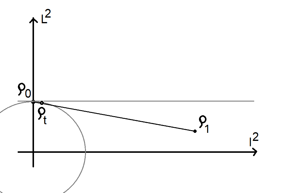
Figure 1. Contradiction in the proof of Proposition 7.2.

Indeed,

$${\rm mass}(\rho_{t})-{\rm mass}(\rho_{0})\sim 2t\int_{S}\rho_{0}(\rho_{1}-\rho_{0})d\sigma,\quad t\to 0.$$

But

$$\int_{S}\rho_{0}\rho_{1}\,d\sigma\leq\left({\rm mass}(\rho_{0})\right)^{1/2}\left({\rm mass}(\rho_{1}|_{S})\right)^{1/2}<{\rm mass}(\rho_{0})=\int_{S}\rho_{0}^{2}d\sigma,$$

and so ${\rm mass}(\rho_{t})<{\rm mass}(\rho_{0})$ for small $t>0$. This contradicts the assumption that $\rho_{0}$ is extremal for $\Gamma$ and concludes the proof of Proposition 7.2. ∎

References

- [Bo88] B. Bojarski, Remarks on Sobolev imbedding inequalities, Complex analysis, Joensuu 1987, 52–68, Lecture Notes in Math., 1351, Springer, Berlin, 1988.
- [Bo11] M. Bonk, Uniformization of Sierpiński carpets in the plane, Invent. math. 186 (2011), 559–665.
- [BM13] M. Bonk, S. Merenkov, Quasisymmetric rigidity of square Sierpínski carpets, Ann. of Math. 177 (2013), 591–643.
- [BF14] B. Branner, N. Fagella, Quasiconformal surgery in holomorphic dynamics. With contributions by X. Buff, S. Bullett, A. L. Epstein, P. Haïssinsky, C. Henriksen, C. L. Petersen, K. M. Pilgrim, T. Lei, M. Yampolsky. Cambridge Studies in Advanced Mathematics, 141. Cambridge University Press, Cambridge, 2014.
- [FM12] B. Farb, D. Margalit, A primer on mapping class groups. Princeton Math. Ser., 49. Princeton University Press, Princeton, NJ, 2012, xiv+472 pp.
- [HM79] J. Hubbard, H. Masur, Quadratic differentials and foliations, Acta Math. 142 (1979), no. 3-4, 221–274.
- [He01] J. Heinonen, Lectures on analysis on metric spaces, Springer-Verlag, New York, 2001.
- [Je57] J. A. Jenkins, On the existence of certain general extremal metrics, Ann. of Math. (2) 66 (1957), 440–453.
- [KM10] F. Kwakkel, V. Markovic, Topological entropy and diffeomorphisms of surfaces with wandering domains, Ann. Acad. Sci. Fenn. Math. 35 (2010), no. 2, 503–513.
- [Sch95] O. Schramm, Transboundary extremal length, J. Anal. Math., 66 (1995), 307–329.
- [St84] K. Strebel, Quadratic differentials, Ergeb. Math. Grenzgeb. (3), 5. Springer-Verlag, Berlin, 1984, xii+184 pp.
- [Su78] D. Sullivan, On the ergodic theory at infinity of an arbitrary discrete group of hyperbolic motions, Riemann surfaces and related topics: Proceedings of the 1978 Stony Brook Conference (State Univ. New York, Stony Brook, N.Y., 1978), pp. 465–496, Ann. of Math. Stud., 97, Princeton Univ. Press, Princeton, N.J., 1981.
- [Tu80] P. Tukia, On two-dimensional quasiconformal groups, Ann. Acad. Sci. Fenn. Ser. A I Math. 5 (1980), no. 1, 73–78.
- [Yo80] K. Yosida, Functional analysis, Sixth edition. Grundlehren der Mathematischen Wissenschaften, 123. Springer-Verlag, Berlin-New York, 1980.