Fourier-Laplace transforms in polynomial Ornstein-Uhlenbeck volatility models

Abstract

We consider the Fourier-Laplace transforms of a broad class of polynomial Ornstein-Uhlenbeck (OU) volatility models, including the well-known Stein-Stein, Schöbel-Zhu, one-factor Bergomi, and the recently introduced Quintic OU models motivated by the SPX-VIX joint calibration problem. We show the connection between the joint Fourier-Laplace functional of the log-price and the integrated variance, and the solution of an infinite dimensional Riccati equation. Next, under some non-vanishing conditions of the Fourier-Laplace transforms, we establish an existence result for such Riccati equation and we provide a discretized approximation of the joint characteristic functional that is exponentially entire. On the practical side, we develop a numerical scheme to solve the stiff infinite dimensional Riccati equations and demonstrate the efficiency and accuracy of the scheme for pricing SPX options and volatility swaps using Fourier and Laplace inversions, with specific examples of the Quintic OU and the one-factor Bergomi models and their calibration to real market data.

JEL Classification:

G13, C63, G10.

Keywords:

Stochastic volatility, Derivative pricing, Fourier methods, Riccati equations, SPX-VIX calibration

1 Introduction

Fourier inversion techniques hold a pivotal role in stochastic volatility modeling, particularly in the context of option pricing and hedging (Andersen and Andreasen [8], Carr and Madan [10], Eberlein, Glau, and Papapantoleon [16], Fang and Oosterlee [19], Lewis [26], Lipton [27]). They offer the dual advantage of significantly reducing computational time while maintaining a remarkable degree of accuracy, especially when compared to standard Monte Carlo methods. When it comes to model calibration, the applicability of Fourier methods is paramount, as thousands of derivatives across various maturities and strikes need to be evaluated simultaneously in real time.

Despite their numerical advantage, Fourier techniques have traditionally been confined to specific continuous stochastic volatility models where the characteristic function of the log-price is known in (semi)-closed form. These models usually exhibit Markovian affine structures in the sense of Duffie, Filipović, and Schachermayer [14] such as the renowned Heston [24], Stein-Stein [32] and Schöbel-Zhu [30] models, together with some of their non-Markovian Volterra counterparts (Abi Jaber [1, 2], Abi Jaber, Larsson, and Pulido [5], Cuchiero and Teichmann [11], El Euch and Rosenbaum [18], Gatheral and Keller-Ressel [22]). The key ingredient in all these models is to compute the characteristic function of the log-price by solving a specific system of deterministic Riccati equation.

More recently, Fourier techniques have also found applications in Signature volatility models in Abi Jaber and Gérard [3] and Cuchiero, Gazzani, Möller, and Svaluto-Ferro [12], where the volatility process is modeled as a linear functional of the path-signature of semi-martingales (e.g. a Brownian motion). In such models, certain characteristic functionals have been related to non-standard infinite dimensional system of Riccati ordinary differential equation (ODE). However, there exists no general theory regarding the existence of solutions for such equations, except for the specific result in Cuchiero, Svaluto-Ferro, and Teichmann [13, Proposition 6.2] which provides the existence of a solution to the infinite dimensional ODE for the case of the characteristic function of powers of a single Brownian motion modulo a non-vanishing condition of the characteristic function. The primary challenge comes from the intricate questions on analyticity of the logarithm of the characteristic function. Furthermore, numerically solving these equations poses challenges due to their stiffness and complexity. This forms our primary motivation: to establish theoretical results within a specific framework for a larger class of Riccati equations related to integrated quantities of power series of Ornstein-Uhlenbeck processes and to develop more suitable numerical schemes.

We demonstrate that Fourier techniques can be effectively extended to a broad class of flexible models previously considered infeasible as they fall beyond the conventional class of affine diffusions, including the celebrated one-factor Bergomi model (Bergomi [9], Dupire [15]) that has been shown to fit well to the SPX smiles and the recently introduced Quintic Ornstein-Uhlenbeck (OU) model of Abi Jaber, Illand, and Li [7], which has demonstrated remarkable capabilities in fitting jointly the SPX-VIX volatility surface for maturities between one week to three months supported by extensive empirical studies on more than 10 years of data in Abi Jaber and Li [4], Abi Jaber, Illand, and Li [6].

We refer to the class of models covered in this paper as the class of polynomial OU models, where the volatility of the log-price, denoted by $\sigma$, is defined as a power series of an Ornstein-Uhlenbeck process. Our three main theoretical results regarding the joint Fourier-Laplace functional of the log-price and integrated variance process are:

1. A verification result on the expression of the joint Fourier-Laplace functional in terms of a solution to an infinite dimensional system of Riccati ODE in Theorem 3.2,

2. The existence of a solution to such a system of ODE modulo a non-vanishing condition of the joint characteristic functional in Theorem 3.5,

3. An approximation procedure for the joint Fourier-Laplace functional in terms of exponentially entire expressions in Theorem 3.13.

On the practical side, we devise a numerical scheme to solve this system of infinite dimensional (stiff) Riccati equations making the application of Fourier pricing for models such as the one-factor Bergomi and the quintic OU models usable in practice. We demonstrate the efficiency and accuracy of the scheme for pricing SPX options and volatility swaps using Fourier and Laplace inversions. We also successfully calibrate using Fourier techniques the Quintic OU and the one-factor Bergomi models on real market data to highlight the stability and robustness of our numerical method across a wide range of realistic parameters values. We provide a Python notebook implementation here: https://colab.research.google.com/drive/1VCVyN1qQmLgOWjOy4fbWftyDqEQdm5n5?usp=sharing.

The paper is organised as follows: in Section 2, we introduce the class of polynomial OU volatility models. In Section 3, we present our three main theoretical results. In Section 4, we design a numerical scheme for solving the infinite dimensional Riccati ODE and test our scheme on pricing SPX vanilla options and volatility swaps for the one-factor Bergomi and quintic OU volatility models of various maturities and calibrate both models using real market data. Proofs of theorems discussed in Section 3 are collected in Section 5 onwards.

Notations. For a power series $q$, we denote by $q_{k}$ the coefficients of $x^{k}$, i.e. $q(x)=\sum_{k=0}^{\infty}q_{k}x^{k}$. We denote by $|q|$ the absolute power series of $q$, i.e. $|q|(x)=\sum_{k=0}^{\infty}|q_{k}|x^{k}$. We remark that $|q|_{k}=|q_{k}|$. It is well-known that if $p$ and $q$ have an infinite radius of convergence, then $p(x)q(x)=\sum_{k=0}^{\infty}(p*q)_{k}x^{k}$ also has an infinite radius of convergence, with $(p*q)_{k}:=\sum_{l=0}^{k}p_{l}q_{k-l}$. Unless stated otherwise, we will assume that all power series in this paper have infinite radius of convergence. Moreover, we specify that the term continuity means joint continuity when applied to a function taking $(t,x)$ as variables. For example, a function $f:[0,T]\times\mathbb{R}\to\mathbb{C}$ is $C^{\infty}$ in $x$ if all its space derivatives in $x$ exist and are continuous in $(t,x)$. We also adopt the following notations for the partial derivatives: $f_{t}=\frac{\partial f}{\partial t},f_{x}=\frac{\partial f}{\partial x},f_{xx}=\frac{\partial^{2}f}{\partial x^{2}}$ when they exist. We say that a function $f:{\mathbb{R}}\to\mathbb{C}$ is (real)-entire on ${\mathbb{R}}$, if it is equal to a power series $q$ (with infinite radius of convergence), that is for all $x\in{\mathbb{R}}$, $f(x)=\sum_{k=0}^{\infty}q_{k}x^{k}.$ We say that it is (complex)-entire when ${\mathbb{R}}$ is replaced by $\mathbb{C}$. Clearly, any real-entire function admits a complex-entire extension. When there is no-ambiguity, we will simply use the word entire. We say that a function does not vanish if it is non-zero at each point of its domain.

2 Polynomial Ornstein-Uhlenbeck volatility models

We consider the class of polynomial Ornstein-Uhlenbeck (OU) models for a stock price $S$ with the stochastic volatility process $\sigma$ expressed as a power series of an OU process $X$:

$$dS_{t} =S_{t}\sigma_{t}dB_{t},\quad S_{0}>0,$$ (2.1)

$$\sigma_{t} =g_{0}(t)p(X_{t}),\quad p(x)=\sum_{k=0}^{\infty}p_{k}x^{k},$$

$$dX_{t} =(a+bX_{t})dt+cdW_{t},\quad X_{0}\in{\mathbb{R}},$$

with $a,b,p_{k}\in\mathbb{R}$, $c\neq 0$, $B=\rho W+\sqrt{1-\rho^{2}}W^{\perp}$ and $\rho\in[-1,1]$. Here $(W,W^{\perp})$ is a two-dimensional Brownian motion on a risk-neutral filtered probability space $(\Omega,\mathcal{F},(\mathcal{F}_{t})_{t\geq 0},\mathbb{Q})$ satisfying the usual conditions. The deterministic bounded input curve $g_{0}:[0,T]\to\mathbb{R}_{{+}}$ allows the model to match certain term structures of volatility, e.g. the forward variance curve since we have for $g_{0}(t):=\sqrt{\xi_{0}(t)/{\mathbb{E}}[p^{2}(X_{t})]}$:

$$\mathbb{E}\left[\int_{0}^{t}\sigma^{2}_{s}ds\right]=\int_{0}^{t}\xi_{0}(s)ds,\quad t\geq 0.$$ (2.2)

The real-valued coefficients $(p_{k})_{k\geq 0}$ are such that the power series $p$ has infinite radius of convergence, i.e. $\sum_{k=0}^{\infty}|p_{k}||x|^{k}<\infty$ for all $x\in{\mathbb{R}}$ and $\int_{0}^{T}{\mathbb{E}}[p^{2}(X_{s})]ds<\infty$ so that the stochastic integral is well-defined. This is the case for instance when $p$ is a finite polynomial or the exponential function. These two specifications already provide several interesting models used in practice:

• Stein-Stein [32] and Schöbel-Zhu [30] model: $p(x)=x$;

• Bergomi model [9, 15]: $p(x)=\exp(x)$;

• Quintic OU model [7]: $p(x)=p_{0}+p_{1}x+p_{3}x^{3}+p_{5}x^{5},\quad p_{0},p_{1},p_{3},p_{5}\geq 0$.

We will consider the following class of power series $p$ for which $\int_{0}^{T}{\mathbb{E}}[p^{2}(X_{s})]ds<\infty$.

Definition 2.1.

A power series $p:x\mapsto\sum_{k=0}^{\infty}p_{k}x^{k}$ is said to be negligible to double factorial if the power series $\sum_{k=0}^{\infty}(k-1)!!p_{k}x^{k}$ has an infinite radius of convergence, i.e.

$$\limsup_{k\rightarrow\infty}(|p_{k}|(k-1)!!)^{\frac{1}{k}}=0,$$

with the convention $(-1)!!=0!!=1$.

By Definition 2.1, a power series $p$ negligible to double factorial also has infinite radius of convergence. This allows us to show that our class of polynomial Ornstein-Uhlenbeck volatility models (2.1) is well-posed in Proposition 2.3. For this we need a simple lemma about the absolute power series which will be useful later.

Lemma 2.2.

_

1. for all $x\in{\mathbb{R}}$, $|p(x)|\leq|p|(|x|)$ and $|p|$ is monotonically increasing on ${\mathbb{R}}^{+}$;

2. for all $x,y,z\geq 0$, $|p|(x+y+z)\leq(|p|(3x)+|p|(3y)+|p|(3z)).$

Proof.

$(i)$ is obvious; for $(ii)$, it suffices to notice that $(x+y+z)^{k}\leq\frac{1}{3}((3x)^{k}+(3y)^{k}+(3z)^{k})\leq((3x)^{k}+(3y)^{k}+(3z)^{k})$. ∎

Proposition 2.3.

Let $g_{0}:[0,T]\to{\mathbb{R}}$ be a measurable and bounded function. Let $p$ be a power series with infinite radius of convergence such that $p^{2}$ is negligible to double factorial. Then,

$$\int_{0}^{T}\mathbb{E}[p^{2}(X_{t})]dt<\infty,$$ (2.3)

so that the stochastic integral $\int_{0}^{\cdot}\sigma_{s}dB_{s}$, with $\sigma_{s}=g_{0}(s)p(X_{s})$, is well-defined and

$$S_{t}=S_{0}\exp\left(-\frac{1}{2}\int_{0}^{t}\sigma_{s}^{2}ds+\int_{0}^{t}\sigma_{s}dB_{s}\right),\quad t\geq 0,$$ (2.4)

is the unique strong solution to (2.1).

Proof.

Under (2.3), it is straightforward to obtain that the unique strong solution $S$ to (2.1) is given by (2.4). It suffices to prove (2.3). For this, we note that the explicit solution of $X$ is given by

$$X_{t}=e^{{b}t}X_{0}+a\int_{0}^{t}e^{{b}(t-s)}ds+c\int_{0}^{t}e^{{b}(t-s)}dW_{s}.$$ (2.5)

We set $w(t):=a\int_{0}^{t}e^{{b}(t-s)}ds$, which is a deterministic continuous function of $t$, and $\widetilde{W}_{t}:=c\int_{0}^{t}e^{{b}(t-s)}dW_{s}$, which is a Gaussian random variable $\sim\mathcal{N}(0,c^{2}\frac{e^{2bt}-1}{2b})$ for $t\in[0,T]$. Applying Lemma 2.2 yields

$$\left|\int_{0}^{T}|p^{2}|\left(e^{bs}X_{0}+w(s)+\widetilde{W}_{s}\right)ds\right| \leq\int_{0}^{T}|p^{2}|\left(e^{bs}|X_{0}|+|w(s)|+|\widetilde{W}_{s}|\right)ds$$ (2.6)

$$\leq\int_{0}^{T}\sum_{k=0}^{\infty}|p^{2}|_{k}\left((3e^{bs}|X_{0}|)^{k}+|3w(s)|^{k}+|3\widetilde{W}_{s}|^{k}\right)ds,$$ (2.7)

and since $e^{bs}\leq e^{|b|T}$ with $w(s)$ bounded in $[0,T]$, there exists a constant $C_{T}\geq 0$ such that

$$\int_{0}^{T}\sum_{k=0}^{\infty}|p^{2}|_{k}\left((3e^{bs}|X_{0}|)^{k}+|3w(s)|^{k}+|3\widetilde{W}_{s}|^{k}\right)ds\leq\int_{0}^{T}\sum_{k=0}^{\infty}|p^{2}|_{k}\left(|3e^{|b|T}|X_{0}|^{k}+(3C_{T})^{k}+|{3\widetilde{W}_{s}}|^{k}\right)ds.$$ (2.8)

By assumption, $p^{2}$ has an infinite radius of convergence, then so does $|p^{2}|$, therefore

$$\sum_{k=0}^{\infty}|p^{2}|_{k}|3e^{|b|T}|X_{0}|^{k}<\infty,\quad\sum_{k=0}^{\infty}|p^{2}|_{k}(3C_{T})^{k}<\infty,$$ (2.9)

and thus we only need to prove

$$\int_{0}^{T}\mathbb{E}[|p^{2}|({|3\widetilde{W}_{t}|})]dt<\infty.$$

The random variable $3\widetilde{W}_{t}$ is Gaussian with bounded variance in $[0,T]$, so there exists a constant $C>0$ such that $\mathbb{E}[{|3\widetilde{W}_{t}|}^{k}]=\mathbb{E}[|CZ|^{k}]$ for all $t\in[0,T]$, where $Z$ is a standard normal variable. Given $\mathbb{E}[|Z|^{k}]\leq(k-1)!!$, hence

$$\mathbb{E}[|p^{2}|(C|Z|)]\leq\sum_{k=0}^{\infty}|p^{2}|_{k}(k-1)!!C^{k}<\infty,$$

since $p^{2}$ is negligible to double factorial. This completes the proof. ∎

Remark 2.4.

In Proposition 2.3, $p^{2}$ needs to be negligible to double factorial. As we will see later in Lemma 6.3 below, the square of a power series negligible to double factorial is also negligible to double factorial. Hence $p$ negligible to double factorial is sufficient for Proposition 2.3 to hold.

Example 2.5.

Polynomials of finite degree (e.g. the Stein-Stein and the Quintic OU models) and the exponential function (e.g. the one-factor Bergomi model) are clearly negligible to double factorial. For the exponential function $p(x)=e^{\varepsilon x},\varepsilon>0$, it suffices to observe that $\lim_{k\rightarrow\infty}(\frac{\varepsilon^{k}(k-1)!!}{k!})^{\frac{1}{k}}=\lim_{k\rightarrow\infty}(\frac{\varepsilon^{k}}{k!!})^{\frac{1}{k}}=0$. However, the function $p(x)=e^{\varepsilon x^{2}}$ is not negligible to double factorial. Indeed, $\limsup_{k\rightarrow\infty}(|p_{k}|(k-1)!!)^{\frac{1}{k}}=\sqrt{2\varepsilon}$. In particular, if $b>0$, then the expectation of $p(X_{t})$ does not exist for all $t\geq\frac{1}{2c^{2}\epsilon}$.

3 The joint Fourier-Laplace transform

Our goal is to compute the joint Fourier-Laplace transform of the log-price and integrated variance

$$\mathbb{E}\left[\exp\left(\int_{t}^{T}g_{1}(T-s)d\log S_{s}+\int_{t}^{T}g_{2}(T-s)\sigma_{s}^{2}ds\right){\ \Big{|}\ }\mathcal{F}_{t}\right],\quad t\leq T,$$

for some complex-valued functions $g_{1},g_{2}:[0,T]\to\mathbb{C}$.

Remark 3.1.

If $g_{1},g_{2}$ are measurable functions $[0,T]\to\mathbb{C}$, such that $\Re(g_{1})=0,\Re(g_{2})\leq 0$, and $p^{2}$ is negligible to double factorial, then the exponential above exists and with modulus of at most $1$, so that the conditional expectation is well-defined.

It follows from the Markov property of $X$ that the above conditional expectation can be reduced to computing the deterministic measurable function $F:[0,T]\times{\mathbb{R}}\to\mathbb{C}$ given by

$$F(t,x):=\mathbb{E}\left[\exp\left(\int_{t}^{T}g_{1}(T-s)d\log S_{s}+\int_{t}^{T}g_{2}(T-s)\sigma_{s}^{2}ds\right){\ \Big{|}\ }X_{t}=x\right].$$ (3.1)

We will present three main results related to the computation of the characteristic functional $F$ in (3.1). The first result can be seen as a verification result and uncovers an affine structure in infinite dimension in terms of the powers $(1,X,X^{2},X^{3},\ldots)$ by making a connection with infinite dimensional Riccati deterministic equations (Theorem 3.2 and Corollary 3.6). The second result is concerned with the existence of a solution to the infinite dimensional Riccati deterministic equation (Theorem 3.5). The last result provides an approximation procedure for obtaining the characteristic functional (Theorem 3.13).

3.1 A verification result

Our first main result uncovers an affine structure in infinite dimension expressed in powers $(1,X,X^{2},\ldots)$ and makes a connection with the following system of infinite dimensional deterministic Riccati equations:

$$\psi_{k}^{\prime}(t) =\Big{(}g_{2}(t)+\frac{g_{1}(t)}{2}(g_{1}(t)-1)\Big{)}g_{0}^{2}(T-t)(p*p)_{k}$$ (3.2)

$$+bk\psi_{k}(t)+a(k+1)\psi_{k+1}(t)+\frac{c^{2}(k+2)(k+1)}{2}\psi_{k+2}(t)$$ (3.3)

$$+\frac{c^{2}}{2}(\widetilde{\psi}(t)*\widetilde{\psi}(t))_{k}+\rho g_{1}(t)g_{0}(T-t)c(p*\widetilde{\psi}(t))_{k},\quad\widetilde{\psi}_{k}(t):=(k+1)\psi_{k+1}(t),$$ (3.4)

$$\psi_{k}(0) =0.$$ (3.6)

Theorem 3.2.

Let $g_{0}:[0,T]\to{\mathbb{R}}$, $g_{1},g_{2}:[0,T]\to\mathbb{C}$ be measurable and bounded functions. Let $p$ be a power series with infinite radius of convergence such that $p^{2}$ is negligible to double factorial. Assume that there exists a continuously differentiable solution $(\psi_{k})_{\geq 0}$ to the system of infinite dimensional Riccati equations (3.6) such that the power series $\sum_{k\geq 0}\sup_{t\in[0,T]}|\psi_{k}(t)|x^{k}$ has an infinite radius of convergence. Define the process

$$U_{t}=\sum_{k\geq 0}\psi_{k}(T-t)X_{t}^{k}+\int_{0}^{t}g_{1}(T-s)d\log S_{s}+\int_{0}^{t}g_{2}(T-s)\sigma_{s}^{2}ds.$$ (3.7)

Then the process $M:=\exp(U)$ is a local martingale. If in addition $M$ is a true martingale, then the following expression holds for the joint characteristic functional $F$ given in (3.1):

$$F(t,x)=\exp\left(\sum_{k\geq 0}\psi_{k}(T-t)x^{k}\right),\quad t\leq T.$$ (3.8)

Proof.

The proof is given in Section 5. ∎

Remark 3.3.

Theorem 3.2 is in the spirit of [13, Theorem 5.5] which provides a similar verification result for the characteristic function of (real)-entire functions of solutions to stochastic differential equations with (real)-entire coefficients. Contrary to [13, Theorem 5.5], Theorem 3.2 deals with time-integrated quantities.

A possible strategy for obtaining the representation (3.8) would involve verifying the assumptions outlined in Theorem 3.2. These assumptions include ensuring the existence of a solution for the system of Riccati equations (3.4)-(3.6), such that the power series $(\psi_{k})_{k\geq 0}$ has infinite radius of convergence; together with proving that the local martingale $M$ is a true martingale. The latter can typically be achieved by arguing, for instance, that $\sum_{k\geq 0}\Re(\psi_{k}(t))x^{k}\leq 0$ to obtain that $M$ is uniformly bounded by $1$ whenever $g_{1},g_{2}$ are purely imaginary for instance.

In the specific case of the Stein-Stein model, i.e. when $p$ is an affine function, these assumptions are comparatively easier to confirm, as highlighted in the next example.

Example 3.4.

In the case of the classical Stein-Stein model [32], the volatility process process is defined as:

$$\sigma_{t}=g_{0}(t)X_{t}.$$

This is equivalent to (2.1) by setting $p_{1}=1$ and $p_{k}=0$ for $k\neq 1$. Notice the convolution term $(p*p)_{k}=1$ for $k=2$ and zero otherwise. In this case, the infinite dimensional Riccati equations (3.6)-(3.4) reduce to the following:

$$\psi_{0}^{\prime}(t) =a\psi_{1}(t)+c^{2}\psi_{2}(t)+\frac{c^{2}}{2}\psi_{1}^{2}(t),$$ (3.9)

$$\psi_{1}^{\prime}(t) =b\psi_{1}(t)+2a\psi_{2}(t)+2c^{2}\psi_{1}(t)\psi_{2}(t)+\rho g_{1}(t)g_{0}(T-t)c\psi_{1}(t),$$ (3.10)

$$\psi_{2}^{\prime}(t) =\Big{(}g_{2}(t)+\frac{g_{1}(t)}{2}(g_{1}(t)-1)\Big{)}g_{0}^{2}(T-t)$$ (3.11)

$$+2b\psi_{2}(t)+2c^{2}\psi_{2}^{2}(t)+2\rho g_{1}(t)g_{0}(T-t)c\psi_{2}(t),$$ (3.12)

$$\psi_{k}(0) =0,\quad k\in\{0,1,2\},$$ (3.14)

$$\psi_{k} \equiv 0,\quad k\geq 3,$$ (3.15)

which is a system of standard finite-dimensional Riccati equations whose existence is well-known whenever $g_{1},g_{2}$ are such that

$$\Re\Big{(}g_{2}(t)+\frac{g_{1}(t)}{2}(g_{1}(t)-1)\Big{)}\leq 0,\quad t\leq T.$$

Hence the characteristic functional of the classical Stein-Stein model is affine in $(1,X,X^{2})$:

$$F(t,x)=\exp\left(\psi_{0}(T-t)+\psi_{1}(T-t)x+\psi_{2}(T-t)x^{2}\right),\quad t\leq T,$$ (3.16)

for which $\psi_{0},\psi_{1}$ and $\psi_{2}$ can even be solved explicitly when $g_{0},g_{1}$ and $g_{2}$ are constants, see [28].

Obtaining the representation (3.8) under the Stein-Stein model can be attributed to the finite number of terms, i.e. $(\psi_{0},\psi_{1},\psi_{2})$ of the Riccati equations, involved in the sum. However, when dealing with an infinite sum, a notable challenge arises in proving that the log of the characteristic functional $\log F$ is entire in the variable $x$ on ${\mathbb{R}}$. In Section 3.2, we show how to generate a solution for the system of infinite-dimensional Riccati equations modulo a non-vanishing condition of $\log F$. In Section 3.3, we provide an expression for the characteristic functional using approximation arguments where the approximations are entire functions thanks to the Gaussianity of the process $X$.

In Section 4, we numerically illustrate the validity of Fourier pricing in the context of the Bergomi and Quintic OU models using the representation (3.8). Readers interested in the numerical implementation can jump directly to Section 4.

3.2 Existence for the Riccati equations

Our second main result generates a solution to the infinite dimensional system of Riccati equations (3.4)-(3.6) by differentiating the logarithm of the characteristic functional $F$:

$$\psi_{k}(t):=\left.\frac{1}{k!}\partial_{x}^{k}\log F({T-t},x)\right|_{x=0},\quad t\geq 0.$$

This requires the logarithm of a complex-valued function, see Appendix B for its precise definition.

Theorem 3.5.

Fix $g_{0}:[0,T]\to{\mathbb{R}}$, $g_{1},g_{2}:[0,T]\to\mathbb{C}$ continuously differentiable such that $\Re(g_{1})=0$ and $\Re(g_{2})\leq 0$. Let $p$ be a power series negligible to double factorial. Then, $F$ in (3.1) is well-defined for any $t\leq T$, $x\in{\mathbb{R}}$ and $(t,x)\mapsto F(t,x)$ is continuous. If in addition $F$ does not vanish on $[0,T]\times{\mathbb{R}}$, then $\log F$ can be defined as in Definition B.5. Furthermore, $\log F$ is $C^{\infty}$ in $x$ and $C^{1}$ in $t$. In particular, the family of functions

$$\psi_{k}(t)=\left.\frac{1}{k!}\partial_{x}^{k}\log F({T-t},x)\right|_{x=0},\quad t\geq 0,\quad k\geq 0,$$ (3.17)

solves the system of Riccati ODEs (3.4)-(3.6).

Proof.

The proof is given in Section 6. ∎

Theorem 3.5 establishes the existence of a solution to the Riccati ODEs (3.4)-(3.6) when the coefficients are real as shown in the following corollary.

Corollary 3.6.

Fix $g_{0}:[0,T]\to{\mathbb{R}}$, $g_{1}=0$ and $g_{2}:[0,T]\to\mathbb{{\mathbb{R}}}_{-}$ continuously differentiable. Let $p$ be a power series negligible to double factorial. Then, $\log F$ is $C^{\infty}$ in $x$ and $C^{1}$ in $t$ and the family of functions $(\psi_{k})_{k\geq 0}$ given by (3.17) solves the system of Riccati ODEs (3.4)-(3.6).

Proof.

In this case, $F$ reduces to the Laplace transform of the integrated variance:

$$F(t,x)={\mathbb{E}}\left[\exp\left(\int_{t}^{T}g_{2}(T-s)\sigma_{s}^{2}ds\right){\ \Big{|}\ }X_{t}=x\right],$$

which shows that $F>0$ and that it trivially satisfies the non-vanishing condition on $[0,T]\times{\mathbb{R}}$ in Theorem 3.5, so that an application of Theorem 3.5 yields the result. ∎

Remark 3.7.

Theorem 3.5 is in the spirit of [13, Proposition 6.2], which provides the existence of a solution to the infinite dimensional ODE for the case of the characteristic function of powers of a single Brownian motion modulo similar assumptions. In contrast, Theorem 3.5 deals with more involved time-integrated quantities which requires a more delicate analysis.

Although Theorem 3.5 does not establish that $\log F(t,\cdot)$ is entire, its analyticity can be inferred from the properties of solutions to parabolic partial differential equations (PDEs).

Remark 3.8.

In order to prove Theorem 3.5, we establish the following PDE for $f(t,x)=F(t,x)\exp(v(t)q(x))$ in Theorem of 6.11:

$$\begin{cases}f_{t}(t,x)+f_{x}(t,x)(a+bx)+\frac{1}{2}c^{2}f_{xx}(t,x)+f(t,x)\sum_{i=1}^{3}u_{i}(t)p_{i}(x)=0,\\ f(T,x)=\exp(v(T)q(x)).\end{cases}$$

where $v,u_{i}$ are continuous and $p_{i}$ are analytic functions. Following [17, Theorem 6.2 in Section II.2.], given that functions $u_{i}(t)$ are continuous in $[0,T]$, $a+bx,p_{i}(x)$ are bounded, Hölder continuous and analytic in variable $x$ within any open bounded set of ${\mathbb{R}}$, one would obtain that $f(t,\cdot)$ is analytic. Notice that $\exp(v(t)q(\cdot))$ is also analytic, then so is $F(t,\cdot)$. Since analyticity is a local property, if $F$ does not vanish, then $\log F(t,\cdot)$ is also analytic. Therefore, we can deduce a local representation: for any $t\leq T$, there exists $r_{t}>0$ such that

$$F(t,x)=\exp\left(\sum_{k=0}^{\infty}\psi_{k}(T-t)x^{k}\right),\quad x\in(-r_{t},r_{t}),$$

where the $(\psi_{k})_{k\geq 0}$ are defined by (3.17). In our case, both $p_{i}$ and $q$ are not only analytic but also entire. Extending the proof of analyticity using PDE techniques to establish that $F(t,\cdot)$ is entire might be possible, and that will lead to a global representation as in (3.8). However, this needs a more delicate analysis at the PDE level, diverging from our probabilistic approach that allowed us to obtain a global representation in terms of approximations by exponentially entire functions, see Theorem 3.13 below. Such a question holds independent interest for PDEs in its own right.

3.3 The Fourier-Laplace transform by approximation

Our third main result provides an approximation procedure for the characteristic functional $F$. The main idea is to approximate the Riemann sum on the sample paths of the Ornstein-Uhlenbeck process $X$ to exploit an underlying Gaussian density in finite dimension.

For this, we need first to get rid of the stochastic integrals and express them in terms of functions of $X_{T}$ and Lebesgue’s integrals on $(X_{s})_{s\leq T}$. This is done by combining Itô’s Lemma and the Romano-Touzi conditioning trick [29] in the next Lemma.

Lemma 3.9.

For $p$ negligible to double factorial, $g_{0}:[0,T]\to{\mathbb{R}}$, $g_{1},g_{2}:[0,T]\to\mathbb{C}$ continuously differentiable with ${\Re(g_{1})=0},\Re(g_{2})\leq 0$, there exists power series $q,p_{i},i=1,2,3$ with infinite radius of convergence, and functions $v,u_{i},i=1,2,3$ such that:

$$F(t,x)=\mathbb{E}\left[\exp\left(\int_{t}^{T}\sum_{i=1}^{3}u_{i}(s)p_{i}(X_{s})ds+v(T)q(X_{T})-v(t)q(X_{t})\right){\ \Big{|}\ }X_{t}=x\right].$$ (3.18)

In addition, $u_{i},v$ are continuous on $[0,T]$, $\Re(u_{1})\leq 0,\Re(u_{2}),\Re(u_{3}),\Re(v)=0$, $p_{1}=p^{2}$ such that $p_{i},q$ are all negligible to double factorial.

Proof.

The proof and the precise expressions of $u_{i},v,p_{i},q$ are given in Appendix A. ∎

We now introduce $F_{n}$ the discretized version of $F$.

Definition 3.10.

For $\mu_{n}=\frac{T}{n}\sum_{i=0}^{n-1}\delta_{\frac{iT}{n}}$, where $\delta_{t}$ is the Dirac mass at a point $t$, we define the function

$$F_{n}(t,x):=\mathbb{E}\left[\exp\left(\int_{t}^{T}\sum_{i=1}^{3}u_{i}(s)p_{i}(X_{s})\mu_{n}(ds)+v(T)q(X_{T})-v(t)q(X_{t})\right){\ \Big{|}\ }X_{t}=x\right].$$ (3.19)

Definition 3.11.

Given an entire function $g$ on ${\mathbb{R}}$, we define the extension of $g$ to the complex plane by $g_{c}(z)=\sum_{0}^{\infty}\frac{g^{(k)}(0)}{k!}z^{k},z\in\mathbb{C}$.

Remark 3.12.

Given an entire function $g$ on ${\mathbb{R}}$, the power series $\sum_{k=0}^{\infty}\frac{g^{(k)}(0)}{k!}x^{k}$ has infinite radius of convergence, so does $\sum_{k=0}^{\infty}\frac{g^{(k)}(0)}{k!}z^{k}$, thus $g_{c}(z)$ is well-defined in $\mathbb{C}$, and is entire on $\mathbb{C}$.

Theorem 3.13.

Suppose that $p$ is negligible to double factorial, $g_{0}:[0,T]\to{\mathbb{R}}$, $g_{1},g_{2}:[0,T]\to\mathbb{C}$ continuously differentiable such that $\Re(g_{1})=0,\Re(g_{2})\leq 0$, then $F_{n}(t,\cdot)$ as specified in Definition 3.10 is well-defined and entire in $x\in\mathbb{R}$. If in addition, the extension of $F_{n}(t,\cdot)$ to the complex plane $(F_{n}(t,\cdot))_{c}$ does not vanish for all $n\in\mathbb{N}$ and $t\leq T$, then, $\log F_{n}$ is entire in $x\in\mathbb{R}$ such that

$$F_{n}(t,x)=\exp\left(\sum_{k\geq 0}\psi_{n,k}(T-t)x^{k}\right),\quad t\leq T,$$ (3.20)

and

$$F(t,x)={\lim_{n\to\infty}F_{n}(t,x)},$$ (3.21)

where for all $n\in\mathbb{N}$, the family of functions $\psi_{n,k}$ is defined by

$$\psi_{n,k}(t) =\phi_{n,k}(t)-\rho g_{1}(t)g_{0}(T-t)\frac{p_{k-1}}{ck},\quad k\geq 1,$$ (3.22)

$$\psi_{n,0}(t) =\phi_{n,0}(t),$$ (3.23)

where the family $\phi_{n,k}$ solves a (step-wise) ‘discretized’ system of Riccati ODEs:

$$\phi_{n,k}^{\prime}(t) =bk\phi_{n,k}(t)+a(k+1)\phi_{n,k+1}(t)+\frac{c^{2}(k+2)(k+1)}{2}\phi_{n,k+2}(t)$$

$$\quad+\frac{c^{2}}{2}(\widetilde{\phi}_{n}(t)*\widetilde{\phi}_{n}(t))_{k},\quad\widetilde{\phi}_{n,k}=(k+1)\phi_{n,k+1},\quad\frac{nt}{T}\notin\{0,1,2,\ldots,n\}$$

$$\phi_{n,k}(t) ={\lim_{s\rightarrow t^{-}}\phi_{n,k}(s)}+\frac{T}{n}\sum_{i=1}^{3}u_{i}(T-t)(p_{i})_{k},\quad\frac{nt}{T}\in\{1,2,\ldots,n\}$$

$$\phi_{n,k}(0) =v(T)q_{k}$$

Proof.

The proof is given in Section 7. ∎

Remark 3.14.

One of the features of Theorem 3.13 is to obtain that the functions $F_{n}(t,\cdot)$ are entire in $x\in\mathbb{R}$ with no additional assumptions. Unfortunately, $\log F_{n}(t,\cdot)$ inherits this property only when the extension of $F_{n}(t,\cdot)$ to the complex plane $(F_{n}(t,\cdot))_{c}$ does not vanish, see Lemma B.3. The requirement of $F_{n}$ being non-vanishing on the real line is not enough, see Remark B.4. For this reason, we could not obtain a Corollary of Theorem 3.13 without the non-vanishing condition to deal with Laplace transforms as we did in Corollary 3.6.

4 Numerical illustration

4.1 Numerical scheme for high-dimensional Riccati equations

In this section, we show how to solve the infinite dimensional Riccati equations $\psi$ in (3.4)-(3.6) numerically for derivative pricing and hedging. The idea is to solve a truncated version of the ODE by assuming $\psi_{k}\approx 0,k>M$ for some integer $M$.

Even the truncated version of the infinite dimensional system of Riccati equations can be extremely difficult to solve. Standard techniques such as the Runge–Kutta methods usually fail to solve the ODE, especially when the parameters $b$ and $c$ in (2.1) are large. For example, see [13, Figures 2 and 3] for other attempts to a similar problem.

We present a customized algorithm that combines variation of constants and the implicit Euler scheme. For this section alone, all matrix and vector indices will start from 0. With some abuse of notation, we re-write the Riccati ODE (3.6) in the following matrix form:

$$\psi^{\prime}(t) =P(t)+A\psi(t)+Q\psi(t)+\frac{c^{2}}{2}(\widetilde{\psi}(t)*\widetilde{\psi}(t))+l(t)N\psi(t),$$ (4.1)

with $\psi(t)$ denoting the vector $(\psi_{0}(t),\psi_{1}(t),\ldots)^{\top}$ and $\psi^{\prime}(t)$ the vector of element-wise derivative of $\psi(t)$. $P(t)$ is a vector with it’s $k^{th}$ element being $\Big{(}g_{2}(t)+\frac{g_{1}(t)}{2}(g_{1}(t)-1)\Big{)}g_{0}^{2}(T-t)(\alpha*\alpha)_{k}$ for $k\in\{0,1,\ldots\}$. $A$ is a diagonal matrix with its diagonal $A_{k,k}=bk$. $Q$ is an upper triangular matrix with $Q_{k,k+1}=a(k+1)$, $Q_{k,k+2}=c^{2}(k+1)(k+2)/2$ and zero elsewhere. The term $(\widetilde{\psi}(t)*\widetilde{\psi}(t))$ denotes the discrete convolution of the vectors $\widetilde{\psi}(t)$, with its $k^{th}$ element given by $(\widetilde{\psi}(t)*\widetilde{\psi}(t))_{k}$. Finally, $N$ is a matrix with $N_{j,k}=kp_{j+1-k}$ where $p_{m}$ denotes the power series coefficient such that $p_{m}=0$ whenever $m<0$, with $l(t)$ collecting the term $c\rho g_{1}(t)g_{0}(T-t)$.

Variation of constants gives:

$$\psi(t_{i+1}) =e^{A\Delta t}\psi(t_{i})+\int_{t_{i}}^{t_{i+1}}e^{A(t_{i+1}-s)}P(s)ds+\int_{t_{i}}^{t_{i+1}}e^{A(t_{i+1}-s)}Q\psi(s)ds$$ (4.2)

$$+\frac{c^{2}}{2}\int_{t_{i}}^{t_{i+1}}e^{A(t_{i+1}-s)}(\widetilde{\psi}(s)*\widetilde{\psi}(s))ds+\int_{t_{i}}^{t_{i+1}}e^{A(t_{i+1}-s)}l(s)N\psi(s)ds,$$

with $\Delta=t_{i+1}-t_{i}$. By truncating the vector $\psi$ up to some level $M$ and assuming $(\psi_{k})_{k>M}=0$, we approximate the solution of $\psi(t_{i+1})$ in (4.2) by the following quasi-implicit scheme:

$$\psi(t_{i+1}) \approx e^{A\Delta t}\psi(t_{i})+G_{\Delta}P(t_{i})+G_{\Delta}Q\psi(t_{i+1})$$

$$+\frac{c^{2}}{2}G_{\Delta}(\widetilde{\psi}(t_{i})*\widetilde{\psi}(t_{i+1}))+G_{\Delta}l(t_{i})N\psi(t_{i+1}),$$

where $G_{\Delta}=\int_{t_{i}}^{t_{i+1}}e^{A(t_{i+1}-s)}ds$ is a diagonal matrix with $G_{k,k}=(e^{b(k-1)\Delta}-1)/(b(k-1)),1<k\leq M+1$ and $G_{1,1}=\Delta$. Similarly, $Q$ and $N$ are now $(M+1)\times(M+1)$ matrices as defined above, with $\psi$ and $P(t_{i})$ both vectors of dimension $M+1$ .

For the quadratic term $(\widetilde{\psi}(t_{i})*\widetilde{\psi}(t_{i+1}))$, we define

$$R^{(i)}\widetilde{\psi}(t_{i+1}):=(\widetilde{\psi}(t_{i})*\widetilde{\psi}(t_{i+1})),$$

where $R^{(i)}$ is a $(M+1)\times(M+1)$ matrix with $R^{(i)}_{j,k}=(j+2-k)k\psi_{{}_{j+2-k}}(t_{i}),(\psi_{{}_{z}}(t_{i}))_{z<0}=0$. We can now solve $\psi$ iteratively by:

$$\psi(t_{i+1}) \approx J^{-1}\Big{(}e^{A\Delta t}\psi(t_{i})+G_{\Delta}P(t_{i})\Big{)},$$

where $J=\bigg{(}I-G_{\Delta}\Big{(}\frac{c^{2}}{2}R^{(i)}+l(t_{i})N+Q\Big{)}\bigg{)}$. Detailed implementation of our algorithm can be found in a Python notebook here: https://colab.research.google.com/drive/1VCVyN1qQmLgOWjOy4fbWftyDqEQdm5n5?usp=sharing.

Lemma 4.1.

Assume that $\Re(\psi)\leq 0$, the matrix $J$ is invertible.

Proof.

Since $\Re(\psi)\leq 0$, the matrix $G_{\Delta}\Big{(}\frac{c^{2}}{2}R^{(i)}+l(t_{i})N+Q\Big{)}\bigg{)}$ is a upper triangular matrix, where the real part of the its diagonal is less than zero. Thus $J$ is also an upper triangular matrix with non-zero diagonal elements, thus completes the proof. ∎

Matrix $Q$ contains very large coefficients resulting from the term $\Big{(}c^{2}(k+2)(k+1)/2\Big{)}$ when $k$ is large. This term introduces numerical instability so we capped $(k+2)(k+1)$ to some level $k_{max}^{2}$ to ensure the scheme does not blown up.

We first test our algorithm on the term ${\mathbb{E}}[\exp(-\frac{W_{t}^{4}}{4!})]$ considered in [13, Figures 2 and 3], which can be expressed by the solution of a particular case of the Riccati ODE in (3.4)-(3.6) with initial condition $\psi_{4}(0)=-1/4!$, $(a,b,g_{1},g_{2})=0$ and $c=1$. The reference value can be computed via a numerical integration quadrature with respect to the Gaussian density, allowing us to evaluate our algorithm’s performance. Figure 1 illustrate numerical convergence in terms of $M$, with step size $n=100$ and $k_{max}=15$ fixed. We clearly observe the instability of the Runge-Kutta scheme with increasing truncation $M$, whereas the scheme we propose remains stable with the increase of $M$.

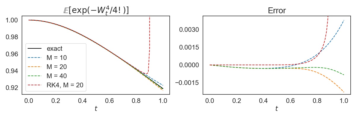
Figure 1: Numerical solution of ${\mathbb{E}}[\exp(-\frac{W_{t}^{4}}{4!})]$ with different values of $M$ using our algorithm vs. the exact solution. For comparison the explicit Runge-Kutta 4 solution with $M=20$ are added in red.

4.2 Pricing SPX derivatives via Fourier

Our numerical scheme gives us direct access to the characteristic function of $\log S$ to price derivatives via Fourier inversion techniques, using the expression (3.8) with $g_{2}(t)=0$ and $g_{1}(t)=iu$, for $u\in\mathbb{R}$. Specifically, we show how one can price European options via Fourier techniques for the Quintic Ornstein-Uhlenbeck Model [7] and the one-factor Bergomi model [9, 15]. This also serves as a numerical validation of the representation (3.8).

There are several Fourier inversion techniques available in the literature to price European-style Vanilla call and put options. Here we adapt the pricing formula suggested in [26] which involves only one integral to evaluate:

$$C_{t}(S_{t},K,T):={\mathbb{E}}\left[(S_{T}-K)^{+}|\mathcal{F}_{t}\right]=S_{t}-\frac{K}{\pi}\int_{0}^{\infty}\Re\left[e^{\left(iu+\frac{1}{2}\right)k_{t}}\varphi\left(u-\frac{i}{2}\right)\right]\frac{du}{u^{2}+\frac{1}{4}},$$ (4.3)

where $C_{t}(S_{t},K,T)$ denotes the European call option price with strike $K$ and maturity $T-t$, $k_{t}:=\log(K/S_{t})$ is the log-moneyness and $\varphi(u):=F(t,x)$ the Fourier-Laplace transform of $\log({S_{T}}/{S_{t}})$ by fixing $g_{1}\equiv iu$ and $g_{2}\equiv 0$. We use the the representation of $F(t,x)$ in (3.8) and compute the improper integral numerically via the Gauss-Laguerre quadrature, which has been demonstrated to be efficient, see [3, 25].

To speed up the computation of $C_{t}$, we add a control variate to reduce the number of evaluation of $\varphi(u)$ for different $u$:

$$C_{t}(S_{t},K,T)=\widehat{C}_{t}(S_{t},K,T)-\frac{K}{\pi}\int_{0}^{\infty}\Re\left[e^{\left(iu+\frac{1}{2}\right)k_{t}}\left(\varphi\left(u-\frac{i}{2}\right)-\widehat{\varphi}\left(u-\frac{i}{2}\right)\right)\right]\frac{du}{u^{2}+\frac{1}{4}},$$ (4.4)

where $\widehat{C}_{t}(S_{t},K,T)$ is the appropriate call price of the control variate and $\widehat{\varphi}\left(u\right)$ is the Fourier-Laplace transform of $\log({S_{T}}/{S_{t}})$ of the control variate.

In this section, we choose the Heston model as the control variate, which admits a closed form characteristic function that is also affine in its state variables, see [24]. The Heston model parameters can be efficiently selected via a standard optimization algorithm such that the difference between $\varphi\left(u-\frac{i}{2}\right)$ and $\widehat{\varphi}\left(u-\frac{i}{2}\right)$ is minimized. Of course, other control variates with explicit characteristic functions such as the Black & Scholes model can also be used.

4.2.1 Quintic Ornstein-Uhlenbeck volatility model

The volatility process $\sigma_{t}$ under the Quintic OU Model takes the form of:

$$\sigma_{t} =\sqrt{\frac{\xi_{0}(t)}{{\mathbb{E}}\left[p(X_{t})^{2}\right]}}p(X_{t}),\quad p(x)=p_{0}+p_{1}x+p_{3}x^{3}+p_{5}x^{5},$$ (4.5)

$$X_{t} =\varepsilon^{\alpha}\int_{0}^{t}e^{\alpha\varepsilon^{-1}(t-s)}dW_{s},$$

with $\varepsilon>0$ and $\alpha\leq 0$. The non-negative coefficients $p_{0},p_{1},p_{3},p_{5}\geq 0$ $(p_{2}=p_{4}=0)$ ensure a negative leverage effect as well as the martingality of $S$ whenever $\rho\leq 0$, see [7] . The particular parametrization with $X$ means $a=0,b=\alpha\varepsilon^{-1}$ and $c=\varepsilon^{\alpha}$ from (2.1). This model has shown to produce remarkable joint fits to both SPX and VIX implied volatility surfaces [6, 7].

Since $X$ is an OU process which can be simulated exactly, one could be tempted to use Monte Carlo to estimate the SPX derivatives with appropriate control variates. However, the calibrated values of $\varepsilon$ are usually very small and $\alpha$ is negative, pushing the model effectively into a fast regime with large mean reversion of order $\alpha\varepsilon^{-1}$ and large vol of vol $\varepsilon^{\alpha}$. It is known the standard Euler-scheme for pricing SPX derivatives can reproduce large estimation bias for longer maturities $T$ due to the highly erratic paths of $\sigma$, requiring finer step size or other asymptotic approximation techniques [20, 21]. Pricing via Fourier methods hence presents an attractive alternative given the increased efficiency and accuracy. To demonstrate, we choose the following parameters: $\rho=-0.65$, $\alpha=-0.6$, $(p_{0},p_{1},p_{3},p_{5})=(0.01,1,0.214,0.227)$, $\xi_{0}(t)=0.025$, $\varepsilon=1/52$ which are typical values one can expect from calibrating the model to SPX and VIX smiles from [7]. Figure 2 shows the convergence of SPX implied volatility of different maturities as the truncation level $M$ increases:

Figure 2: SPX implied volatility of different maturities in the quintic OU model, computed with our algorithm with different level $M$. Dotted red lines are Monte-Carlo 95% interval computed with 500,000 simulations and $n=10,000$ number of steps per maturity slice.

4.2.2 One-factor Bergomi model

The one-factor Bergomi model [9, 15] assumes $\sigma_{t}$ to be log-normal:

$$\sigma_{t} =\sqrt{\xi_{0}(t)}\exp{\left(\frac{1}{2}\eta X_{t}-\frac{1}{4}\eta^{2}{\mathbb{E}}(X_{t})\right)},$$ (4.6)

$$X_{t} =\varepsilon^{\alpha}\int_{0}^{t}e^{\alpha\varepsilon^{-1}(t-s)}dW_{s},$$

with $\varepsilon>0$ and $\alpha\leq 0$. Similar to quintic OU model before, we have $a=0,b=\alpha\varepsilon^{-1}$ and $c=\varepsilon^{\alpha}$. We now approximate the exponential as a truncated sum up to level $N$:

$$\widetilde{\sigma}_{t} =\sqrt{\frac{\xi_{0}(t)}{{\mathbb{E}}[p(X_{t})^{2}]}}p(X_{t}),\quad p(X_{t})=\sum_{k=0}^{N}p_{k}X_{t}^{k},\quad p_{k}=\frac{\eta^{k}}{2^{k}k!},$$ (4.7)

where $\widetilde{\sigma}_{t}$ in converges to $\sigma_{t}$ in (4.6) when sending $N\rightarrow\infty$. We now fix $\rho=-0.7,\varepsilon=1/52,\alpha=-0.7,\eta=1.2,\xi_{0}(t)=0.025$ for the numerical experiment and set $N=8$. Figure 3 shows that our numerical scheme quickly converges to Monte-Carlo estimates of the original one-factor Bergomi model:

Figure 3: SPX implied volatility of different maturities in the one-factor Bergomi model, computed with our algorithm with different level $M$. Dotted red lines are Monte-Carlo 95% interval computed with 500,000 simulations and $n=10,000$ number of steps per maturity slice.

4.3 Pricing $q$-volatility swaps via Laplace inversion

The $q$-volatility swap rate $K_{q}$ is defined by:

$$K_{q}:={\mathbb{E}}\left[\left(\frac{1}{T}\int_{0}^{T}\sigma_{s}^{2}ds\right)^{q}\right],\quad q\in[0,1].$$

For the case of a standard volatility swap (i.e. $q=1/2$), one can price the swap rate $K^{q}$ via the following inverse Laplace transform [31]:

$$K_{\frac{1}{2}}={\mathbb{E}}\left[\left(\frac{1}{T}\int_{0}^{T}\sigma_{s}^{2}ds\right)^{1/2}\right]=\frac{1}{2\sqrt{\pi}}\int_{0}^{\infty}\frac{1-\tilde{F}(u)}{u^{3/2}}du,$$

where $\tilde{F}(u)=F(t,x)$ from (3.1) by setting $g_{1}\equiv 0$ and $g_{2}(t)\equiv-u/T$ using the presentation (3.8). Again, we can accelerate the computation via a control variate, for example the Black & Scholes control variate:

$$K_{\frac{1}{2}}=\sigma_{BS}+\frac{1}{2\sqrt{\pi}}\int_{0}^{\infty}\frac{\widetilde{F}_{BS}(u)-\tilde{F}(u)}{u^{3/2}}du,$$

with $F_{BS}(u)=\exp(-u\sigma_{BS}^{2})$ where $\sigma_{BS}$ is an arbitrary level of volatility that can be fixed upfront.

Compared to the previous section, we are even more confident of our numerical scheme thanks to Corollary 3.6. For demonstration purposes, we use the same model parameters for the Quintic Ornstein-Uhlenbeck and the one-factor Bergomi model as per the previous section, and adopt a parametric forward variance curve in the form of $\xi_{0}(t)=V_{0}e^{-kt}+V_{\infty}(1-e^{-kt})$ with $V_{0}=0.025,k=5$ and $V_{\infty}=0.06$.

Figure 4 shows the volatility swaps of the two models computed by inverse Laplace transform with truncation level $M=32$ vs. that computed by Monte-Carlo with 400,000 simulations and 10,000 steps:

Figure 4: Volatility swaps under the Quintic OU model (left) and the one-factor Bergomi model (right) for maturities up to 2 years, using the same parameter values as in the previous section.

4.4 Model calibration to market data via Fourier

The family of polynomial OU volatility models allows fast pricing of VIX futures and VIX options via numerical integration of the payoff with respect to the standard Gaussian density, see [7]. Together with fast Fourier pricing, this opens doors to joint calibration to SPX and VIX smiles. This section also serves the purpose of highlighting the stability of our numerical discretization scheme combined with Fourier inversion in a calibration procedure where a large number of evaluations of the characteristic function are needed for a wide range of realistic model parameters and Fourier variables.

In a nutshell, the calibration of a model involves minimizing the mean square error between prices coming from the model vs. that from market data. Without going too much into the details, we first demonstrate the capability of the quintic OU model (4.5) to jointly calibrate two slices of maturities of SPX smiles together with one slice of maturity of the VIX smile, with calibrated parameters $\rho=-0.6763,\alpha=-0.6821,(p_{0},p_{1},p_{3},p_{5})=(0.0202,1.3332,0.0578,0.0071)$ and fixed $\varepsilon=1/52$: with $\xi_{0}(t)$ coming directly from market data:

Figure 5: Quintic OU model (green lines) jointly calibrated to the SPX and VIX smiles (bid/ask in blue/red) on 23 October 2017 via Fourier using the Nelder-Mead optimization algorithm. The truncation level of the Riccati solver is set at $M=32$.

Next, we showcase the calibration results of the one-factor Bergomi model (4.6) on four slices of maturities of SPX smiles between around 1 week to 3 months, with calibrated parameters $\eta=1.1416,\rho=-0.6744,\alpha=-0.7377$ and fixed $\varepsilon=1/52$:

Figure 6: One-factor Bergomi model (green lines) calibrated to the SPX smiles (bid/ask in blue/red) on 23 October 2017 via Fourier using the Nelder-Mead optimization algorithm. The truncation level of the Riccati solver is set at $M=32$.

The market data of SPX and VIX volatility surface is purchased from the CBOE website https://datashop.cboe.com/. For more calibration examples under the quintic OU and the one-factor Bergomi models, please refer to the the Appendix C.

5 Proof of Theorem 3.2

We first introduce a lemma to justify the use of Itô’s formula to the series $\sum_{k\geq 0}\psi_{k}(T-t)X_{t}^{k}$.

Lemma 5.1.

Under the condition of Theorem 3.2, $h(t,x):=\sum_{k\geq 0}\psi_{k}(T-t)x^{k}$ is $C^{2}$ in $x$ and $C^{1}$ in $t$, with $h_{x}(t,x)=\sum_{k\geq 0}(k+1)\psi_{k+1}(T-t)x^{k}$, $h_{xx}(t,x)=\sum_{k\geq 0}(k+2)(k+1)\psi_{k+2}(T-t)x^{k}$, $h_{t}(t,x)=\sum_{k\geq 0}-\psi^{\prime}_{k}(T-t)x^{k}$.

Proof.

First, $|\psi_{k}(T-t)x^{k}|\leq\sup_{t\in[0,T]}|\psi_{k}(t)||x|^{k}$, and $\sum_{k\leq 0}\sup_{t\in[0,T]}|\psi_{k}(t)||x|^{k}<\infty$. So $h(t,x)=\sum_{k\geq 0}\psi_{k}(T-t)x^{k}$ is well defined. In addition, if we restrict $x$ in a bounded set of ${\mathbb{R}}$, then $h^{n}(t,x):=\sum_{k=0}^{n}\psi_{k}(T-t)x^{k}$ is continuous and converges uniformly to $h(t,x)$ when $n\rightarrow\infty$, so $h(t,x)$ is continuous.

Notice that the domain of convergence for $\sum_{k\leq 0}\sup_{t\in[0,T]}|\psi_{k}(t)|x^{k}<\infty$ is ${\mathbb{R}}$, then so is $\sum_{k\geq 0}\psi_{k}(T-t)x^{k}$. So $h_{x}(t,x),h_{xx}(t,x)$ are well-defined, continuous and have the expression as the statement for the same reason as for $h(t,x)$.

To treat $h_{t}(t,x)$, we should at first prove that $\sum_{k}\sup_{t\in[0,T]}|\psi^{\prime}_{k}(t)|x^{k}$ has also an infinite radius of convergence.

Indeed, using the Riccati expression (3.4), we only have to check that we have an infinite radius of convergence for

$$\sum_{k\geq 0}\sup_{t\in[0,T]}|a_{t,k}|x^{k},$$ (5.1)

where $a_{t,k}$ is among $(p*p)_{k},k\psi_{k}(t),(k+1)\psi_{k+1},\frac{(k+1)(k+1)}{2}\psi_{k+1},(\widetilde{\psi}(t)*\widetilde{\psi}(t))_{k},(p*\widetilde{\psi}(t))_{k}$.

By assumption and Cauchy–Hadamard Theorem, we know that $\limsup_{n\rightarrow\infty}(\sup_{t\in[0,T]}|\psi_{n}(t)|)^{\frac{1}{n}}=0$ and thus we obtain that when $a_{t,x}=k\psi_{k}(t),(k+1)\psi_{k+1}=\widetilde{\psi}(t)_{k},\frac{(k+1)(k+2)}{2}\psi_{k+2}$, (5.1) has an infinite radius of convergence.

Also, for two power series $\sum_{n=0}^{\infty}a_{n}x^{n}$ and $\sum_{n=0}^{\infty}b_{n}x^{n}$ both with infinite radius of convergence, their product $\sum_{n=0}^{\infty}(a*b)_{n}x^{n}$ also has an infinite radius of convergence. And notice that $(p*p)_{k},(\widetilde{\psi}(t)*\widetilde{\psi}(t))_{k},(p*\widetilde{\psi}(t))_{k}$ are dominated by $(|p|*|p|)_{k},(\sup_{t\in[0,T]}|\widetilde{\psi}(t)|*\sup_{t\in[0,T]}|\widetilde{\psi}(t)|)_{k},(|p|*\sup_{t\in[0,T]}|\widetilde{\psi}(t)|)_{k}$. Thus when $a_{t,k}$ is among $(p*p)_{k},(\widetilde{\psi}(t)*\widetilde{\psi}(t))_{k},(p*\widetilde{\psi}(t))_{k}$, (5.1) has also an infinite radius of convergence. Therefore $\sum_{k}\sup_{t\in[0,T]}|\psi^{\prime}_{k}(t)|x^{k}$ has an infinite radius of convergence, so that $\sum_{k\geq 0}-\psi^{\prime}_{k}(T-t)x^{k}$ also has infinite radius of convergence and converges uniformly when $x$ is in a bounded subset of ${\mathbb{R}}$ and also on $t\in[0,T]$. So $\sum_{k\geq 0}-\psi^{\prime}_{k}(T-t)x^{k}$ is well-defined and also continuous.

Next, notice that $h^{n}_{t}(t,x)=\sum_{k=0}^{n}-\psi^{\prime}_{k}(T-t)x^{k}$ and given the the uniform convergence of both series $\sum_{k\geq 0}-\psi^{\prime}_{k}(T-t)x^{k}$ and $\sum_{k\geq 0}\psi_{k}(T-t)x^{k}$, we deduce that $h_{t}(t,x)=(\sum_{k\geq 0}\psi_{k}(T-t)x^{k})_{t}=\sum_{k\geq 0}-\psi^{\prime}_{k}(T-t)x^{k}.$

∎

Proof of Theorem 3.2.

We first notice that since the power series $\sum_{k}|\psi_{k}(t)|x^{k}$ has an infinite radius of convergence, $U_{t}$ is well-defined for all $t\leq T$.

With Lemma 5.1, we can now apply Itô’s formula on the semimartingale $M$:

$$\frac{dM_{t}}{M_{t}} =dU_{t}+\frac{1}{2}\langle U\rangle_{t},$$ (5.2)

$$dU_{t} =g_{1}(T-t)d\log S_{t}+g_{2}(T-t)\sigma_{t}^{2}dt-\sum_{k}\psi_{k}^{\prime}(T-t)X_{t}^{k}dt$$

$${+\sum_{k}(k+1)\psi_{k}(T-t)X_{t}^{k}dX_{t}+\sum_{k}\frac{1}{2}(k+2)(k+1)\psi_{k}(T-t)X_{t}^{k}d\langle X\rangle_{t}}.$$

Plugging (2.1) into (5.2), we have:

$$dU_{t} =\Bigg{(}\big{(}g_{2}(T-t)-\frac{g_{1}(T-t)}{2}\bigg{)}\sigma_{t}^{2}-\sum_{k}\psi_{k}^{\prime}(T-t)X_{t}^{k}$$ (5.3)

$$+\sum_{k}a(k+1)\psi_{k}(T-t)X_{t}^{k}+\sum_{k}bk\psi_{k}(T-t)X_{t}^{k}+\sum_{k}c^{2}\frac{(k+2)(k+1)}{2}\psi_{k}(T-t)X_{t}^{k}\Bigg{)}dt$$

$$+\bigg{(}\sum_{k}c(k+1)\psi_{k}(T-t)X_{t}^{k}+\rho g_{1}(T-t)\sigma_{t}\bigg{)}dW_{t}+\sqrt{1-\rho^{2}}g_{1}(T-t)\sigma_{t}dW_{t}^{\perp},$$

$$d\langle U\rangle_{t} =\bigg{(}\sum_{k}ck\psi_{k}(T-t)X_{t}^{k}+\rho g_{1}(T-t)\sigma_{t}\bigg{)}^{2}dt+(1-\rho^{2})g_{1}^{2}(T-t)\sigma_{t}^{2}dt.$$

Applying the Cauchy product on the power series $\sum_{k}p_{k}X_{t}^{k}$ leads to

$$\frac{dM_{t}}{M_{t}} =\Big{(}\sum_{k}\Big{[}(g_{2}(T-t)-\frac{g_{1}(T-t)}{2})g_{0}^{2}(t)(p*p)_{k}-\psi_{k}^{\prime}(T-t)+a(k+1)\psi_{k+1}(T-t)$$ (5.4)

$$+bk\psi_{k}(T-t)+\frac{c^{2}(k+2)(k+1)}{2}\psi_{k+2}(T-t)$$

$$+\frac{c^{2}}{2}(\widetilde{\psi}(T-t)*\widetilde{\psi}(T-t))_{k}+\frac{g_{1}^{2}(T-t)g_{0}^{2}(t)}{2}(p*p)_{k}$$

$$+\rho g_{1}(T-t)g_{0}(t)c(p*\widetilde{\psi}(T-t))_{k}\Big{]}X_{t}^{k}\Big{)}dt$$

$$+\bigg{(}\sum_{k}ck\psi_{k}(T-t)X_{t}^{k}+\rho g_{1}(T-t)\sigma_{t}\bigg{)}dW_{t}+\sqrt{1-\rho^{2}}g_{1}(T-t)\sigma_{t}dW_{t}^{\perp}.$$

$M$ is a local martingale if and only if it has zero drift (i.e. $dt$ part is zero a.s.). This is true for all values of $X$ by assumption from (3.4), so that $M$ is a local martingale. Moreover, if $M$ is a true martingale, we have

$$\mathbb{E}\left[\left.\exp\left(\int_{t}^{T}g_{1}(T-s)d\log S_{s}+\int_{t}^{T}g_{2}(T-s)\sigma_{s}^{2}ds\right)\right|\mathcal{F}_{t}\right]$$ (5.5)

$$=\exp\left(\sum_{k\geq 0}\psi_{k}(T-t)X_{t}^{k}\right),\quad t\leq T.$$

which follows from the martingality of $M$ and the assumption of the initial condition of $\psi_{k}$ from (3.6). This completes the proof. ∎

6 Proof of Theorem 3.5

To prove Theorem 3.5, we adopt the representation of $F$ as mentioned in Lemma 3.9:

$$F(t,x)=\mathbb{E}\left[\exp\left(\int_{t}^{T}\sum_{i=1}^{3}u_{i}(s)p_{i}(X_{s})ds+v(T)q(X_{T})-v(t)q(X_{t})\right){\ \Big{|}\ }X_{t}=x\right],$$

where the functions $p_{1}=p^{2},p_{2},p_{3},q$ are all negligible to double factorial and $(u_{1},u_{2},u_{3},v)$ are continuous such that $\Re(u_{1})\leq 0,\Re(u_{2})=\Re(u_{3})=\Re(v)=0$. Consider the following function $f$ defined by:

$$f(t,x): =\mathbb{E}\left[\exp\left(\int_{t}^{T}\sum_{i=1}^{3}u_{i}(s)p_{i}(X_{s})ds+v(T)q(X_{T})\right){\ \Big{|}\ }X_{t}=x\right]$$ (6.1)

$$=F(t,x)\exp(v(t)q(x)),$$ (6.2)

for all $t\leq T$ and $x\in{\mathbb{R}}$. We recall that $f$ is well-defined, since

$$\Re\left(\int_{t}^{T}\sum_{i=1}^{3}u_{i}(s)p_{i}(X_{s})ds+v(T)q(X_{T})\right)=\int_{t}^{T}\Re\left(u_{1}(s)p^{2}(X_{s})\right)ds\leq 0.$$

Our proof is composed of five parts:

• In Subsection 6.1, we start by deriving some properties of power series negligible to double factorial which will be used later.

• In Subsection 6.2, we prove the regularity in $x$ of $f$ given by (6.2), i.e. $f$ is $C^{\infty}$ in $x$ such that the partial derivatives $\frac{\partial^{k}f}{\partial x^{k}}$ are bounded in a sense in preparation for the Feynman-Kac formula in Subsection 6.3.

• In Subsection 6.3, we prove that $f$ solves the associated PDE coming from Feynman-Kac formula. In particular, we prove that $\frac{\partial f}{\partial t}$ indeed exists.

• In Subsection 6.4, we introduce a system of ODE and obtain a solution by comparing the derivatives of all orders of both sides of Feynman-Kac formula at $x=0$.

• In Subsection 6.5, we prove that the system of ODE in Theorem 3.5 has a solution, via a system of ODE introduced in Subsection 6.4.

6.1 Properties of power series negligible to double factorial

We collect some properties of power series that are negligible to double factorial as defined per Definition 2.1.

Given a power series $p(x)=\sum_{k=0}^{\infty}p_{k}x^{k}$, we define the set $\mathcal{A}_{D}(p)$ as the ${\mathbb{R}}$-algebra generated by all higher-order derivatives $\{p,p^{\prime},p^{\prime\prime}\ldots\}$ of $p$:

$$\mathcal{A}_{D}(p):=\left\{\sum_{s=0}^{l}c_{s}f_{s,1}f_{s,2}\cdots f_{s,m_{s}}:l\in\mathbb{N},\ m_{s}\in\mathbb{N},\ c_{s}\in{\mathbb{R}},\ f_{s,i}\in\{p,p^{\prime},p^{\prime\prime}\ldots\}\text{ for every }i\text{ and }s\right\}.$$ (6.3)

Notice that if $m_{s}=0$, then by convention the product $f_{s,1}f_{s,2}\cdots f_{s,m_{s}}=1$.

Remark 6.1.

This definition comes from the calculations of the successive partial derivatives $F_{x},F_{xx},\ldots$ For example, in the simple case when $g_{0}=1,g_{1}=0,g_{2}=-1$, by setting $Z=\exp\left(-\int_{0}^{T-t}p^{2}\left(X_{s}\right)ds\right)$, we have $F(t,x)=\mathbb{E}\left[Z|X_{0}=x\right]$ by the Markov property of $X$. Since we can write $X_{s}=e^{bs}X_{0}+Y_{s}$, where $Y_{s}$ does not depend on $X_{0}$, this means formally, $F_{x}=\mathbb{E}\left[Z_{x}|X_{0}=x\right]$, where $Z_{x}=-Z\int_{0}^{T-t}2e^{bs}pp^{\prime}\left(X_{s}\right)ds$ and $pp^{\prime}\in\mathcal{A}_{D}(p)$ appears. Higher order derivatives like $Z_{xx},Z_{xxx}$ will also formally generate the elements in $\mathcal{A}_{D}(p)$.

Now we prove some properties of power series which are negligible to double factorial. For the lemma below, we recall the convention $(-1)!!=(0)!!=1$. Notice that although the proof is a little cumbersome, the essential idea is the observation that $\ell!!$ behaves like $(\lfloor\frac{\ell}{2}\rfloor)!2^{\frac{\ell}{2}}$ and $\sum_{k=0}^{\ell}{\ell\choose{k}}=2^{\ell}$.

Lemma 6.2.

There exists a constant $C>0$, such that for all $\ell\in\mathbb{N}$, we have that

$$\sum_{k=0}^{\ell}\frac{1}{(k-1)!!(\ell-k-1)!!}\leq\frac{C{\ell}^{3}2^{\frac{\ell}{2}}}{(\ell-1)!!}.$$

Proof.

For $k=0,\ell$, we have $\frac{1}{(k-1)!!(\ell-k-1)!!}=\frac{1}{(\ell-1)!!}$. So we need only to prove that for a constant $C>0$,

$$\sum_{k=1}^{\ell-1}\frac{1}{(k-1)!!(\ell-k-1)!!}=\sum_{k=0}^{\ell-2}\frac{1}{k!!(\ell-2-k)!!}\leq\frac{C{\ell}^{3}2^{\frac{\ell}{2}}}{(\ell-1)!!}.$$ (6.4)

Case 1: $\ell=2\ell_{1}$ is an even number. If $k=2k_{1}$ is an even number, $k!!(\ell-2-k)!!=2^{\ell_{1}-1}k_{1}!(\ell_{1}-1-k_{1})!$. If $k=2k_{1}+1$ is an odd number, $k!!(\ell-2-k)!!=(2k_{1}+1)!!(\ell-3-2k_{1})!!\geq\frac{(2k_{1}+1)!!(\ell-1-2k_{1})!!}{\ell-1-2k_{1}}\geq\frac{(2k_{1})!!(\ell-2-2k_{1})!!}{\ell}=\frac{2^{\ell_{1}-1}k_{1}!(\ell_{1}-1-k_{1})!}{\ell}$. Therefore,

$$\sum_{k=0}^{\ell-2}\frac{1}{k!!(\ell-2-k)!!} \leq\sum_{k_{1}=0}^{\ell_{1}-1}\frac{\ell+1}{2^{\ell_{1}-1}k_{1}!(\ell_{1}-1-k_{1})!}=\frac{\ell+1}{(\ell_{1}-1)!}=\frac{(\ell+1)2^{\ell_{1}-1}}{(\ell-2)!!}$$ (6.5)

$$\leq\frac{(\ell+1)(\ell-1)2^{\ell_{1}-1}}{(\ell-1)!!}\leq\frac{\ell^{2}2^{\frac{\ell}{2}}}{(\ell-1)!!}.$$ (6.6)

Case 2: $\ell=2\ell_{1}+1$ is an odd number, then

$$\sum_{k=0}^{\ell-2}\frac{1}{k!!(\ell-2-k)!!}\leq\sum_{k=0}^{\ell-3}\frac{1}{k!!(\ell-3-k)!!}+\frac{1}{(\ell-2)!!},$$ (6.7)

and since $\ell-3$ is even, as the Case 1, we have, for a constant $C>0$:

$$\sum_{k=0}^{\ell-3}\frac{1}{k!!(\ell-3-k)!!}+\frac{1}{(\ell-2)!!}\leq\frac{(\ell-1)^{2}2^{\frac{\ell-1}{2}}}{(\ell-2)!!}+\frac{1}{(\ell-2)!!}\leq\frac{C\ell^{3}2^{\frac{\ell}{2}}}{(\ell-1)!!}.$$ (6.8)

Therefore there exists constant $C$ such that for all $\ell$, $\sum_{k=0}^{\ell-2}\frac{1}{k!!(\ell-2-k)!!}\leq\frac{C\ell^{3}2^{\frac{\ell}{2}}}{(\ell-1)!!}$. ∎

Lemma 6.3.

The following statements are true.

1. If $p$ is negligible to double factorial, then so is $q(x)=\int_{0}^{x}p(y)dy$.

2. The set of power series which are negligible to double factorial is closed under addition, differentiation, scalar multiplication, and multiplication. Thus if $p$ is negligible to double factorial, then for any $q\in\mathcal{A}_{D}(p)$, $q$ is also negligible to double factorial.

3. If $p(x)=\sum p_{k}x^{k}$ is negligible to double factorial, then so is $q(x)=\sum p_{k}c^{k}x^{k}$, where $c$ is a constant.

4. If $p$ is negligible to double factorial, then so is $|p|$.

Proof.

1. Note that $q(x)=\sum_{k=1}^{\infty}\frac{p_{k-1}}{k}x^{k}$. It follows that

   $$\limsup_{k\rightarrow\infty}(|q_{k}|(k-1)!!)^{\frac{1}{k}} =\limsup_{k\rightarrow\infty}((|p_{k-1}|\frac{(k-1)!!}{k})^{\frac{1}{k-1}})^{\frac{k-1}{k}}$$ (6.9)

   $$\leq\limsup_{k\rightarrow\infty}((|p_{k-1}|(k-2)!!)^{\frac{1}{k-1}})^{\frac{k-1}{k}}=0,$$ (6.10)

   using that $\frac{(k-1)!!}{k}\leq\frac{k!!}{k}=(k-2)!!$.

2. Let $p,q$ be negligible to double factorial and note that $q^{\prime}(x)=\sum_{k=0}^{\infty}(k+1)q_{k+1}x^{k}$. Then,

   $$\limsup_{k\rightarrow\infty}(|q^{\prime}_{k}|(k-1)!!)^{\frac{1}{k}} =\limsup_{k\rightarrow\infty}((|q_{k+1}|(k+1)!!)^{\frac{1}{k+1}})^{\frac{k+1}{k}},$$ (6.11)

   then by $(k+1)!!\leq(k+1)k!!$,

   $$\limsup_{k\rightarrow\infty}(|q^{\prime}_{k}|(k-1)!!)^{\frac{1}{k}} \leq\limsup_{k\rightarrow\infty}((|q_{k+1}|k!!)^{\frac{1}{k+1}})^{\frac{k+1}{k}}(k+1)^{\frac{1}{k}}=0.$$ (6.12)

   By $|a+b|^{\frac{1}{k}}\leq|a|^{\frac{1}{k}}+|b|^{\frac{1}{k}}$, $\limsup_{k\rightarrow\infty}(|q_{k}+p_{k}|(k-1)!!)^{\frac{1}{k}}=0$, and $\limsup_{k\rightarrow\infty}(|cq_{k}|(k-1)!!)^{\frac{1}{k}}=0$ for any constant $c$.

   Next, we will show that $pq$ is again negligible to double factorial. For any $\epsilon>0$, there exists $N$, such that for all $k>N$, we have that $(|q_{k}|(k-1)!!)\leq\epsilon^{k},(|p_{k}|(k-1)!!)\leq\epsilon^{k}$. Therefore there exists constant $C_{\epsilon}$ such that $(|q_{k}|(k-1)!!)\leq C_{\epsilon}\epsilon^{k},(|p_{k}|(k-1)!!)\leq C_{\epsilon}\epsilon^{k}$ for all $k$. Thus by Lemma 6.2,

   $$|(pq)_{l}|=|\sum_{k=0}^{l}p_{k}q_{l-k}|$$ (6.13)

   $$\leq\sum_{k=0}^{l}|p_{k}||q_{l-k}|\leq\sum_{k=0}^{l}\frac{{C_{\epsilon}}^{2}\epsilon^{l}}{(k-1)!!(l-k-1)!!}\leq\frac{{C_{\epsilon}}^{2}C(\sqrt{2}\epsilon)^{l}l^{3}}{(l-1)!!},$$ (6.14)

   thus $\limsup_{l\rightarrow\infty}(|(pq)_{l}|(l-1)!!)^{\frac{1}{l}}\leq\sqrt{2}\epsilon$. Since $\epsilon$ can be any arbitrary positive number, we obtain

   $$\limsup_{l\rightarrow\infty}(|(pq)_{l}|(l-1)!!)^{\frac{1}{l}}=0.$$

   Therefore, $pq$ is also negligible to double factorial.

3. Notice that

   $$\limsup_{k\rightarrow\infty}(|q_{k}|(k-1)!!)^{\frac{1}{k}}=|c|\limsup_{k\rightarrow\infty}(|p_{k}|(k-1)!!)^{\frac{1}{k}}=0.$$

4. It is obvious, since the modulus of $p$ has no impact on the $\limsup_{k\rightarrow\infty}(|p_{k}|(k-1)!!)^{\frac{1}{k}}$.

∎

6.2 Regularity in space

In this subsection, we prove the regularity of $f$ in $x$ given by (6.2), i.e. $f$ is $C^{\infty}$ in $x$ such that the partial derivatives $\frac{\partial^{k}f}{\partial x^{k}}$ are bounded in a sense in preparation for the Feynman-Kac formula in Subsection 6.3.

Theorem 6.4.

The function $f$ given by (6.2) is $C^{\infty}$ in $x$, i.e. the partial derivatives $\frac{\partial^{k}f}{\partial x^{k}}$ exist and are continuous in $(t,x)$, for $k\in\mathbb{N}$. Furthermore, for each $k\in\mathbb{N}$, there exists a power series $q_{k}$ negligible to double factorial and a constant $C_{k}$ independent of $(t,x)$, such that

$$\left|\frac{\partial^{k}f}{\partial x^{k}}(t,x)\right|\leq|q_{k}|(|x|)+C_{k},\quad t\in[0,T],\;x\in{\mathbb{R}}.$$ (6.15)

Before proving Theorem 6.4, we first simplify the expression of $f$ in (6.2) to get rid of the conditioning. Thanks to the Markovianity of $X$, we can write $f$ after a change of variable as:

$$f(t,x) =\mathbb{E}\left[Z(t,x)\right],$$ (6.16)

with

$$Z(t,x):=\exp\bigg{(} \int_{0}^{T-t}\sum_{i=1}^{3}u_{i}(t+s)p_{i}\left(e^{bs}x+w(s)+\widetilde{W}_{s}\right)ds$$ (6.17)

$$\quad\quad+v(T)q(e^{b(T-t)}x+w(T-t)+\widetilde{W}_{T-t})\bigg{)}.$$ (6.18)

Notice $X_{t}=e^{bt}x+w(t)+\widetilde{W}_{t}$ when $X_{0}=x$, with $w(t):=a\int_{0}^{t}e^{{b}(t-u)}du$ and ${\widetilde{{W}}_{t}}:=c\int_{0}^{t}e^{{b}(t-u)}dW_{u}$. From now on, we will consider mainly the representation (6.16) for $f(t,x)$.

The main idea for proving Theorem 6.4 consists in taking successive derivatives in $x$ inside the expectation above and applying the dominated convergence theorem. To illustrate this, we first calculate formally $\frac{\partial f}{\partial x}$. Notice that the derivative in $x$ for the terms inside the exponential of $Z(t,x)$ is:

$$h(x) :=\int_{0}^{T-t}\sum_{i=1}^{3}u_{i}(t+s)e^{bs}p_{i}^{\prime}\left(e^{bs}x+w(s)+\widetilde{W}_{s}\right)ds$$ (6.19)

$$+v(T)e^{b(T-t)}q^{\prime}\left(e^{b(T-t)}x+w(T-t)+\widetilde{W}_{T-t}\right),$$ (6.20)

so that one expects

$$\frac{\partial f}{\partial x}(t,x)=\mathbb{E}\left[h(x)Z(t,x)\right].$$ (6.21)

Notice that $|Z(t,x)|\leq 1$ since the terms inside the exponential of $Z(t,x)$ have a non-positive real part as a result of Lemma 3.9. Therefore we only need to bound $h(x+\theta\Delta x)$ for $\theta\in[0,1]$ and small enough $\Delta x\in{\mathbb{R}}$. Notice that $u_{i},v$ are continuous and thus bounded on $[0,T]$, $e^{bs}$ is also bounded in $[0,T]$, $p_{i}^{\prime},q^{\prime}$ are negligible to double factorial by the statement $(ii)$ of Lemma 6.3. So we only need to bound the expressions of the following form

$$\int_{0}^{t}q\left(e^{bs}x+w(s)+\widetilde{W}_{s}\right)ds\quad\text{and}\quad q\left(e^{bt}x+w(t)+\widetilde{W}_{t}\right),$$ (6.22)

where $q$ is any power series negligible to double factorial.

First of all, we introduce a new definition and a lemma to help bound in a certain sense the quantities in (6.22). We also introduce the notation $\widetilde{W}^{*}_{t}:=\sup_{s\leq t}|\widetilde{W}_{s}|$, which will be useful for applying Doob’s inequality.

Definition 6.5.

We say that a family of processes $(M_{t}(x))_{t\leq T,x\in{\mathbb{R}}}$ is estimable if there exists a power series $q$ negligible to double factorial such that for all fixed $t\in[0,T]$ and $x\in{\mathbb{R}}$,

$$|M_{t}(x)|\leq|q|(|x|)+|q|(\widetilde{W}^{*}_{T}),\quad a.s.$$

We will prove that the expressions in (6.22) are estimable in Proposition 6.7 below. For now, let us first prove that $|q|(|x|)+|q|(\widetilde{W}^{*}_{T})$ is integrable via the following lemma.

Lemma 6.6.

The set of estimable family of processes is closed under addition and multiplication. In addition, for all power series $q$ negligible to double factorial, $\mathbb{E}\left[|q|(\widetilde{W}^{*}_{T})\right]<\infty$. Therefore, if $M_{t}(x)$ is estimable, then there exists a power series $q$ negligible to double factorial and a constant $C$, such that for all $t\in[0,T]$ and $x\in{\mathbb{R}}$, $\mathbb{E}[|M_{t}(x)|]\leq|q|(|x|)+C$.

Proof.

For the first part of this lemma, recall that by the statements $(ii)$ and $(iv)$ of Lemma 6.3, the property of being negligible to double factorial is closed under addition, multiplication, and taking absolute power series. So the set of estimable family of process is obviously closed under addition. For the multiplication, it suffices to use the basic inequality $(a+b)(c+d)\leq a^{2}+b^{2}+c^{2}+d^{2}$.

To show that $\mathbb{E}\left[|q|(\widetilde{W}^{*}_{T})\right]<\infty$, recall $\widetilde{W}_{t}=e^{bt}\int_{0}^{t}e^{-bs}cdW_{s}$, where $\int_{0}^{t}e^{-bs}cdW_{s}$ is a true martingale. There is a positive constant $C_{T}$ such that $\frac{1}{C_{T}}<e^{bt}<C_{T}$ when $0\leq t\leq T$. We use $\overline{W}_{t}$ to denote $\int_{0}^{t}e^{-bs}cdW_{s}$ and $\overline{W}_{t}^{*}$ to denote its maximal process $\sup_{s\leq t}|\overline{W}_{s}|$. By Doob’s maximal inequality for $k\geq 2$,

$$\mathbb{E}\left[(\widetilde{W}^{*}_{T})^{k}\right]\leq C_{T}^{k}\mathbb{E}\left[(\overline{W}^{*}_{T})^{k}\right]\leq C_{T}^{k}\left(\frac{k}{k-1}\right)^{k}\mathbb{E}\left[|{\overline{W}_{T}}|^{k}\right]\leq 4C_{T}^{k}\mathbb{E}\left[|{\overline{W}_{T}}|^{k}\right]\leq 4C_{T}^{2k}\mathbb{E}\left[|{\widetilde{W}_{T}}|^{k}\right].$$

For $k=1$,

$$\mathbb{E}\left[\widetilde{W}^{*}_{T}\right]\leq\frac{1}{2}\left(1+\mathbb{E}\left[(\widetilde{W}^{*}_{T})^{2}\right]\right)\leq 1+4C_{T}^{4}\mathbb{E}\left[({\widetilde{W}_{T}})^{2}\right].$$

Notice that $\widetilde{W}_{T}$ is a centred normal distribution and that the constant $C_{T}$ can be taken large enough so that the variance of ${\widetilde{W}_{T}}$ is smaller than $C_{T}^{2}$. It follows that $\mathbb{E}\left[|{\widetilde{W}_{T}}|^{k}\right]\leq(C_{T}^{2})^{\frac{k}{2}}(k-1)!!$. By modifying a little the coefficients $|q|_{0},|q|_{1},|q|_{2}$ in the power series $|q|$, which does not influence the conclusion, we obtain that $C=4\sum_{k=0}^{\infty}|q|_{k}(k-1)!!C_{T}^{3k}$ satisfies the requirements and is finite, since $q$ is negligible to double factorial.∎

Proposition 6.7.

If $q$ is negligible to double factorial, then the expressions in (6.22) are estimable, and

$$\mathbb{E}\left[\left|\int_{0}^{t}q\left(e^{bs}x+w(s)+\widetilde{W}_{s}\right)ds\right|\right]+\mathbb{E}\left[\left|q\left(e^{bt}x+w(t)+\widetilde{W}_{t}\right)\right|\right]\leq|\tilde{q}|(|x|)+C,\quad t\in[0,T],\;x\in{\mathbb{R}},$$

where $\tilde{q}$ is negligible to double factorial and only depends on $T,q$, and $C$ is a constant.

Proof.

Fix $t\in[0,T]$ and $x\in{\mathbb{R}}$. We first bound $q\left(e^{bt}x+w(t)+\widetilde{W}_{t}\right)$:

$$\left|q\left(e^{bt}x+w(t)+\widetilde{W}_{t}\right)\right| \leq|q|\left(e^{bt}|x|+|w(t)|+|\widetilde{W}_{t}|\right)\leq\sum_{k=0}^{\infty}|q|_{k}\left((3e^{bt}|x|)^{k}+|3w(t)|^{k}+|3\widetilde{W}_{t}|^{k}\right)$$ (6.23)

by Lemma 2.2. Since $e^{bt}$ and $w(t)$ are both bounded in $[0,T]$, there exists a constant $C_{T}\geq 0$ such that

$$\sum_{k=0}^{\infty}|q|_{k}\left((3e^{bt}|x|)^{k}+|3w(t)|^{k}+|3\widetilde{W}_{t}|^{k}\right)\leq \sum_{k=0}^{\infty}|q|_{k}\left(|3C_{T}x|^{k}+(3C_{T})^{k}+|3\widetilde{W}_{t}|^{k}\right)$$ (6.24)

$$\leq |q|(|3C_{T}x|)+|q|(|3C_{T}|)+|q|(3\widetilde{W}^{*}_{T}).$$ (6.25)

Setting $\tilde{q}(x)=|q|(3(C_{T}+1)x)+|q|(|3C_{T}|)$, we get $\left|q\left(e^{bt}x+w(t)+\widetilde{W}_{t}\right)\right|\leq\tilde{q}(|x|)+\tilde{q}(\widetilde{W}^{*}_{T})=|\tilde{q}|(|x|)+|\tilde{q}|(\widetilde{W}^{*}_{T})$. By Lemma 6.3, $|q|$ is also negligible to double factorial, and $\tilde{q}$ is still negligible to double factorial. So $q\left(e^{bt}x+w(t)+\widetilde{W}_{t}\right)$ is estimable. An application of Lemma 6.6 yields the bound for the expectation. Furthermore, the term $\int_{0}^{t}q\left(e^{bs}x+w(s)+\widetilde{W}_{s}ds\right)$ is clearly bounded by $T|\tilde{q}|(|x|)+T|\tilde{q}|(\widetilde{W}^{*}_{T})$. So we can update $\tilde{q}$ to $\tilde{q}(x)=T\vee 1|q|(3(C_{T}+1)x)+T\vee 1|q|(|3C_{T}|)$ to obtain the claimed bound and end the proof. ∎

We have now that $|\int_{0}^{t}q\left(e^{bs}(x+\theta\Delta x)+w(s)+\widetilde{W}_{s}\right)ds|\leq|\tilde{q}|(|x+\theta\Delta x|)+|\tilde{q}|(\widetilde{W}^{*}_{T})\leq|\tilde{q}|(|x|+1)+|\tilde{q}|(\widetilde{W}^{*}_{T})$ since we can choose that $|\Delta x|\leq 1$, $\theta\in[0,1]$ with coefficient of $|\tilde{q}|$ all positive. The dominating function $|\tilde{q}|(|x|+1)+|\tilde{q}|(\widetilde{W}^{*}_{T})$ is integrable. For the term $q\left(e^{bt}(x+\theta\Delta x)+w(t)+\widetilde{W}_{t}\right)$, we can build a dominating function in a similar way.

Going back to (6.21), we now have all the ingredients to apply the dominated convergence theorem when $\Delta x\rightarrow 0$ on

$$\frac{f(t,x+\Delta x)-f(t,x)}{\Delta x}=\mathbb{E}\left[\frac{Z(t,x+\Delta x)-Z(t,x)}{\Delta x}\right]=\mathbb{E}\left[h(x+\theta\Delta x)Z(t,x+\theta\Delta x)\right],$$

where $\theta\in[0,1]$. Recall $h(x)$ from (6.20), and that $|Z(t,x)|\leq 1$ and $u_{i},v$ are bounded, $e^{bs}$ is bounded in $[0,T]$, $p_{i}^{\prime},q^{\prime}$ are negligible to double factorial. Therefore, (6.21) holds. Of course, we would like to prove by induction that

$$\frac{\partial^{k}f}{\partial x^{k}}(t,x)=\mathbb{E}\left[H_{k}(t,x)Z(t,x)\right]$$

holds for all $k\in\mathbb{N}$ to show that $f$ is $C^{\infty}$ in $x$ , where

$$H_{k+1}(t,x)=\frac{\partial H_{k}(t,x)}{\partial x}+H_{k}(t,x)h(x),\quad H_{0}(t,x)=1,\quad H_{1}(t,x)=h(x).$$ (6.26)

To achieve this, we need to prove first that $H_{k}$ are well-defined. Then, similarly to before, we will bound $H_{k}(x)$ so that we can apply by induction the dominated convergence theorem to

$$\lim_{\Delta x\rightarrow 0}\frac{\frac{\partial^{k}f}{\partial x^{k}}(t,x+\Delta x)-\frac{\partial^{k}f}{\partial x^{k}}(t,x)}{\Delta x}$$ (6.27)

$$= \lim_{\Delta x\rightarrow 0}\mathbb{E}\left[\frac{H_{k}(t,x+\Delta x)Z(t,x+\Delta x)-H_{k}(t,x)Z(t,x)}{\Delta x}\right]$$ (6.28)

$$= \lim_{\Delta x\rightarrow 0}\mathbb{E}\left[H_{k+1}(t,x+\theta\Delta x)Z(t,x+\theta\Delta x)\right].$$ (6.29)

For $H_{2}(t,x)$, we need to compute $\frac{\partial h(x)}{\partial x}$, recall that $h(x)$ is just a sum of the Riemann integral of the continuously differentiable function and a differentiable function with respect to $x$ for a fixed $\omega$ outside a null-set. Therefore,

$$\frac{\partial h(x)}{\partial x} =\int_{0}^{T-t}\sum_{i=1}^{3}u_{i}(t+s)e^{2bs}p_{i}^{\prime\prime}\left(e^{bs}x+w(s)+\widetilde{W}_{s}\right)ds$$ (6.30)

$$+v(T)e^{2b(T-t)}q^{\prime\prime}\left(e^{b(T-t)}x+w(T-t)+\widetilde{W}_{T-t}\right).$$ (6.31)

Thus $H_{2}$ can be obtained explicitly, and similarly for $H_{3},H_{4},\ldots,H_{k},\ldots$. This procedure will differentiate many times the function $h(x)$, so it is useful to define:

$$h_{k}(x): =\int_{0}^{T-t}\sum_{i=1}^{3}u_{i}(t+s)e^{kbs}p_{i}^{(k)}\left(e^{bs}x+w(s)+\widetilde{W}_{s}\right)ds$$ (6.32)

$$+v(T)e^{kb(T-t)}q^{(k)}\left(e^{b(T-t)}x+w(T-t)+\widetilde{W}_{T-t}\right).$$ (6.33)

Definition 6.8.

We define the set $\mathcal{A}_{x}(h)$:

$$\mathcal{A}_{x}(h):=\left\{\sum_{s=0}^{l}c_{s}h_{s,1}h_{s,2}\cdots h_{s,m_{s}}:l\in\mathbb{N},\ m_{s}\in\mathbb{N},\ c_{s}\in{\mathbb{R}},\ h_{s,i}\in\{h\}_{k}\text{ for every }i\text{ and }s\right\}.$$ (6.34)

as the ${\mathbb{R}}$-algebra generated by higher order derivatives of the function $h(x)$. We call $h_{k}$ generating elements of $\mathcal{A}_{x}(h)$.

Notice that if $m_{s}=0$, then by convention the product $h_{s,1}h_{s,2}\cdots h_{s,m_{s}}=1$.

In the next Lemma 6.9, we will characterize $H_{k}$ defined in (6.26).

Lemma 6.9.

For every $k\in\mathbb{N}$, the function $H_{k}$ in (6.26) is well-defined. In addition, $H_{k}$ is differentiable in $x$, continuous in $(t,x)$ and estimable.

Proof.

First, note the following three facts:

1. $h(x)=h_{1}(x)$ is a generating element of $\mathcal{A}_{x}(h)$,

2. $H_{0}=1\in\mathcal{A}_{x}(h)$,

3. All generating elements $h_{k}(x)$ of $\mathcal{A}_{x}(h)$ are differentiable in $x$ by applying the Leibniz’s rule, and $\frac{\partial h_{k}(x)}{\partial x}=h_{k+1}(x)$. So if $g\in\mathcal{A}_{x}(h)$, then $\frac{\partial g}{\partial x}$ exists and $\in\mathcal{A}_{x}(h)$.

By induction and noticing that $\mathcal{A}_{x}(h)$ is closed under linear sum and multiplication, $H_{k}$ are well-defined and in $\mathcal{A}_{x}(h)$. For fixed $\omega\in\Omega$ outside a null-set, the generating elements $h_{k}$ are continuous in $(t,x)$ and differentiable in $x$. This implies that $H_{k}$ is also continuous in $(t,x)$ and differentiable in $x$.

We know $u_{i},v$ are continuous (and thus bounded), $e^{kbs}$ is bounded in $[0,T]$, $p_{i}^{(k)},q^{(k)}$ are negligible to double factorial by the statement 2 of Lemma 6.3. By Proposition 6.7, generating elements $h_{k}$ of $\mathcal{A}_{x}(h)$ are estimable. Since $H_{k}\in\mathcal{A}_{x}(h)$ is a linear sum of finite product of generating elements of $\mathcal{A}_{x}(h)$, by Lemma 6.6 $H_{k}$ is also estimable. ∎

We are now ready to prove Theorem 6.4.

Proof of Theorem 6.4.

Take $H_{k}$ as defined in (6.26) which are estimable by Lemma 6.9. By applying Lemma 6.6,the term $H_{k}(t,x)Z(t,x)$ is estimable with its expectation bounded by $|q_{k}|(|x|)+C_{k}$. Using induction, we first notice that for the case $k=0$, $\left|\frac{\partial^{k}f}{\partial x}\right|=|f(t,x)|\leq{\mathbb{E}}[|Z(t,x)|]\leq 1$ which trivially satisfies the inequality in (6.15). Next, suppose that it is true for up to case $k$, recall the definition of $Z$ from (6.18) and that $Z_{x}=hZ$, where $h$ is defined in (6.20). Thus $(H_{k}Z)_{x}=H_{k+1}Z$. Since both $Z$ and $H_{k+1}$ are differentiable in $x$ as per 6.9, by the Mean value theorem:

$$\frac{1}{\Delta x}\Big{(}H_{k}(t,x+\Delta x)Z(t,x+\Delta x)-H_{k}(t,x)Z(t,x)\Big{)}=H_{k+1}(t,x+\theta\Delta x)Z(t,x+\theta\Delta x),$$

where $\theta$ is $\in[0,1]$. Strictly speaking, since $H_{k}Z$ is a complex-valued functions, we need to apply the Mean value on both the real part and imaginary part separately with different $\theta$. However, this does not change the proof at all, so to simplify the notation and discussion, only $\theta$ is used.

By Lemma 2.2, Lemma 6.9 and the fact that $|Z|\leq 1$, and $H_{k+1}(t,x+\theta\Delta x)$ is dominated by $|q_{k+1}|(|x|+1)+|q_{k+1}|(\widetilde{W}^{*}_{T})$ with bounded expectation by Lemma 6.6 if we choose that $|\Delta x|\leq 1$, where $q_{k+1}$ is negligible to double factorial. Applying dominated convergence theorem, for $\Delta x\rightarrow 0$ we have:

$$\frac{\partial^{k+1}f}{\partial x^{k+1}}(t,x) =\mathbb{E}\Bigg{[}H_{k+1}(t,x)Z(t,x)\Bigg{]}.$$ (6.35)

Therefore, for all $k\in\mathbb{N}$, where $q_{k}$ negligible to double factorial and a constant $C_{k}$, we have that (6.15) holds. Finally, for the continuity of $\frac{\partial^{k}f}{\partial x^{k}}(t,x)$, it suffices to notice that before taking the expectation, the random variable $H_{k}(t,x)Z(t,x)$ is continuous with respect to $(t,x)$, Then fixing $(t_{0},x_{0})$, again by Proposition 6.7, Lemma 6.9, its expectation is uniformly bounded with $t\leq T$, and $|x|\leq|x_{0}|+1$ bounded. So again by the dominated convergence theorem and taking the limit at $(t_{0},x_{0})$, the continuity holds.∎

6.3 Feynman-Kac

In this subsection, we derive the Feynman-Kac formula in Theorem 6.11. Since we do not have that $f_{t}$ exists a priori in our setting, we shall prove its existence and obtain the Feynman-Kac formula at the same time.

First, we introduce a lemma which will be useful later.

Lemma 6.10.

Let $z\in\mathbb{C}$ such that $\Re(z)\leq 0$, then $|\exp(z)-1|\leq 3|z|$.

Proof.

We write $z=x+yi$, $x\leq 0$ and $y\in{\mathbb{R}}$. Then $|\exp(z)-1|=|\exp(x+yi)-1|=|\exp(yi)(\exp(x)-1)+\exp(yi)-1|\leq|\exp(x)-1|+|\cos(y)-1|+|\sin(y)|$.

If $x=0$, then $|\exp(x)-1|=0$. If $x<0$, $|\frac{\exp(x)-1}{z}|\leq|\frac{\exp(x)-1}{x}|\leq 1$.

If $y=0$, then $|\cos(y)-1|=0,|\sin(y)|=0$. If $y\neq 0$, $|\frac{\cos(y)-1}{z}|\leq|\frac{\cos(y)-1}{y}|\leq 1$, $|\frac{\sin(y)}{z}|\leq|\frac{\sin(y)}{y}|\leq 1$. ∎

Theorem 6.11.

The function $f$ given by (6.2) and equivalently (6.16) is $C^{\infty}$ in $x$, $C^{1}$ in $t$, and solves the following partial differential equation (PDE):

$$\begin{cases}f_{t}(t,x)+f_{x}(t,x)(a+bx)+\frac{1}{2}c^{2}f_{xx}(t,x)+f(t,x)\sum_{i=1}^{3}u_{i}(t)p_{i}(x)=0,\\ f(T,x)=\exp(v(T)q(x)).\end{cases}$$ (6.36)

Proof.

By Theorem 6.4, $f$ is $C^{\infty}$ in $x$. We will compute the infinitesimal generator

$$\lim_{r\rightarrow 0^{+}}\frac{1}{r}(\mathbb{E}^{x}\left[f(t_{0},X_{r})-f(t_{0},x)\right])$$

in two ways to obtain the PDE and the existence of $f_{t}$ at the same time. Here $\mathbb{E}^{x}$ means the conditional expectation with $X_{0}=x$.

First way: fix $t_{0}$, we compute the quantity using the classical definition of generator. By Itô’s formula:

$$df(t_{0},X_{t})=f_{x}dX_{t}+\frac{1}{2}f_{xx}d\langle X\rangle_{t}=cf_{x}dW_{t}+\left(\frac{1}{2}c^{2}f_{xx}+(a+bX_{t})f_{x}\right)dt.$$ (6.37)

Note that $f_{x},f_{xx}$ are evaluated at $(t_{0},X_{t})$ here. By Theorem 6.4, statement $(ii)$ of Lemma 6.3, $f_{x}(t,x),(a+bx)f_{x}(t,x),f_{xx}(t,x),f_{x}^{2}(t,x)$ are all bounded by $|q|(|x|)+C$, where $q$ is negligible to double factorial. Combining with Proposition 6.7, $\mathbb{E}^{x}\left[\int_{0}^{r}f_{x}^{2}(t_{0},X_{t})dt\right]$ is bounded by $|\tilde{q}|(|x|)+C$ for $r\in[0,T]$, where $\tilde{q}$ is negligible to double factorial. Thus $\int_{0}^{r}cf_{x}(t_{0},X_{t})dW_{t}$ is in $L^{2}$ and is a true martingale for $t\in[0,T]$. Similarly, the Riemann integral $\int_{0}^{r}(\frac{1}{2}c^{2}f_{xx}(t_{0},X_{t})+(a+bX_{t})f_{x}(t_{0},X_{t}))dt$ is estimable with finite expectation. In addition, we have

$$\left|\frac{1}{r}\int_{0}^{r}(\frac{1}{2}c^{2}f_{xx}(t_{0},X_{t})+(a+bX_{t})f_{x}(t_{0},X_{t})dt\right|\leq\sup_{s\in[0,r]}\frac{1}{2}c^{2}|f_{xx}(t_{0},X_{s})|+|(a+bX_{s})f_{x}(t_{0},X_{s})|,$$

where the right hand side is still estimable and dominated by a random variable with finite expectation. By dominated convergence theorem,

$$\lim_{r\rightarrow 0^{+}}\frac{1}{r}(\mathbb{E}^{x}\left[f(t_{0},X_{r})-f(t_{0},x)\right])$$ (6.38)

$$= \lim_{r\rightarrow 0^{+}}\frac{1}{r}\mathbb{E}^{x}\left[\int_{0}^{r}(\frac{1}{2}c^{2}f_{xx}(t_{0},X_{t})+(a+bX_{t})f_{x}(t_{0},X_{t}))dt\right]$$ (6.39)

$$= \frac{1}{2}c^{2}f_{xx}(t_{0},x)+(a+bx)f_{x}(t_{0},x)).$$ (6.40)

Second way: compute the generator $\lim_{r\rightarrow 0^{+}}\frac{1}{r}(\mathbb{E}^{x}\left[f(t_{0},X_{r})-f(t_{0},x)\right])$ directly by applying the Markov property of $X_{t}$. Define $Z_{t}:=\exp(\int_{0}^{t}\sum_{i=1}^{3}u_{i}(T-t+s)p_{i}\left(X_{s}\right)ds)$ and $Y_{t}=v(T)q(X_{t})$, we apply Markov property of $X_{t}$ to the representation of $f(t,x)$ in (6.2), i.e.

$$f(t,x)=\mathbb{E}\left[\exp\left(\int_{0}^{T-t}\sum_{i=1}^{3}u_{i}(t+s)p_{i}(X_{s})ds+v(T)q(X_{T-t})\right){\ \Big{|}\ }X_{0}=x\right],$$ (6.41)

and by Markov property for $r\in[0,t]$,

$$f(t,X_{r})= \mathbb{E}\left[\exp\left(\int_{r}^{T-t+r}\sum_{i=1}^{3}u_{i}(t-r+s)p_{i}(X_{s})ds+v(T)q(X_{T-t+r})\right){\ \Big{|}\ }X_{r}\right].$$ (6.42)

By the tower property of conditional expectation, we have

$$\mathbb{E}^{x}\left[f(t,X_{r})\right]= \mathbb{E}^{x}\left[\mathbb{E}\left[\exp\left(\int_{r}^{T-t+r}\sum_{i=1}^{3}u_{i}(t-r+s)p_{i}(X_{s})ds+v(T)q(X_{T-t+r})\right){\ \Big{|}\ }X_{r}\right]\right]$$ (6.43)

$$= \mathbb{E}^{x}\left[\exp\left(\int_{r}^{T-t+r}\sum_{i=1}^{3}u_{i}(t-r+s)p_{i}(X_{s})ds+v(T)q(X_{T-t+r})\right)\right]$$ (6.44)

$$= \mathbb{E}^{x}\left[Z_{T-t+r}\cdot\exp\left(-\int_{0}^{r}\sum_{i=1}^{3}u_{i}(t-r+s)p_{i}\left(X_{s}\right)ds\right)\exp\left(Y_{T-t+r}\right)\right].$$ (6.45)

Therefore,

$$\frac{1}{r}\left(\mathbb{E}^{x}\left[f\left(t_{0},X_{r}\right)-f(t_{0},x)\right]\right)$$ (6.46)

$$= \frac{1}{r}\mathbb{E}^{x}\left[Z_{T-t_{0}+r}\exp\left(-\int_{0}^{r}\sum_{i=1}^{3}u_{i}(t_{0}-r+s)p_{i}\left(X_{s}\right)ds\right)\exp\left(Y_{T-t_{0}+r}\right)-Z_{T-t_{0}}\exp(Y_{T-t_{0}})\right]$$ (6.47)

$$= \frac{1}{r}\mathbb{E}^{x}\Bigg{[}\exp\left(Y_{T-t_{0}+r}\right)Z_{T-t_{0}+r}-\exp\left(Y_{T-t_{0}}\right)Z_{T-t_{0}}\Bigg{]}$$ (6.48)

$$+ \frac{1}{r}\mathbb{E}^{x}\left[\exp\left(Y_{T-t_{0}+r}\right)Z_{T-t_{0}+r}\left(\exp\left(-\int_{0}^{r}\sum_{i=1}^{3}u_{i}(t_{0}-r+s)p_{i}\left(X_{s}\right)ds\right)-1\right)\right]$$ (6.49)

$$= \frac{1}{r}(f(t_{0}-r,x)-f(t_{0},x))$$ (6.50)

$$+ \frac{1}{r}\mathbb{E}^{x}\left[\exp\left(Y_{T-t_{0}+r}\right)Z_{T-t_{0}+r}\left(\exp\left(-\int_{0}^{r}\sum_{i=1}^{3}u_{i}(t_{0}-r+s)p_{i}\left(X_{s}\right)ds\right)-1\right)\right].$$ (6.51)

Now we want to apply dominated convergence theorem when $r\rightarrow 0^{+}$ to the term

$$\frac{1}{r}\mathbb{E}^{x}\left[\exp\left(Y_{T-t_{0}+r}\right)Z_{T-t_{0}+r}\left(\exp\left(-\int_{0}^{r}\sum_{i=1}^{3}u_{i}(t_{0}-r+s)p_{i}\left(X_{s}\right)ds\right)-1\right)\right].$$

To dominate the term inside the expectation, notice that at first $\Re(Y_{t})=\Re(v(T)q(X_{t}))=0$, thus $|\exp(Y_{T-t_{0}+r})|=1$. In addition,

$$\left|\frac{1}{r}Z_{T-t_{0}+r}\left(\exp\left(-\int_{0}^{r}\sum_{i=1}^{3}u_{i}(t_{0}-r+s)p_{i}\left(X_{s}\right)ds\right)-1\right)\right|$$ (6.52)

$$= \left|\frac{1}{r}\exp\left(\int_{r}^{T-t_{0}+r}\sum_{i=1}^{3}u_{i}(t_{0}-r+s)p_{i}\left(X_{s}\right)ds\right)\left(1-\exp\left(\int_{0}^{r}\sum_{i=1}^{3}u_{i}(t_{0}-r+s)p_{i}\left(X_{s}\right)ds\right)\right)\right|.$$ (6.53)

Since $\Re(u_{1})\leq 0,\Re(u_{2}),\Re(u_{3})=0,p_{1}=p^{2}$, therefore

$$\Re\Big{(}\int_{r}^{T-t_{0}+r}\sum_{i=1}^{3}u_{i}(t_{0}-r+s)p_{i}\left(X_{s}\right)ds\Big{)}=\int_{r}^{T-t_{0}+r}\Re\Big{(}u_{1}(t_{0}-r+s)p_{1}\left(X_{s}\right)\Big{)}ds\leq 0$$

and thus $\Big{|}\exp\left(\int_{r}^{T-t_{0}+r}\sum_{i=1}^{3}u_{i}(t_{0}-r+s)p_{i}\left(X_{s}\right)ds\right)\Big{|}\leq 1$. Therefore we only need to dominate the term

$$\frac{1}{r}\left(\exp\left(\int_{0}^{r}\sum_{i=1}^{3}u_{i}(t_{0}-r+s)p_{i}\left(X_{s}\right)ds\right)-1\right).$$

Since $\Re(\int_{0}^{r}\sum_{i=1}^{3}u_{i}(t_{0}-r+s)p_{i}\left(X_{s}\right)ds)\leq 0$, by Lemma 6.10 we just need to dominate the term

$$\left|\frac{1}{r}\int_{0}^{r}\sum_{i=1}^{3}u_{i}(t_{0}-r+s)p_{i}\left(X_{s}\right)ds\right|\leq\sum_{i=1}^{3}||u_{i}||_{\infty}\sup_{s\in[0,r]}|p_{i}(X_{s})|.$$

Notice $|u_{i}(s)|$ are bounded, $p_{i}$ are negligible to double factorial so $|p_{i}(X_{s})|,s\in[0,T]$ is dominated when conditioned $X_{0}=x$ by Proposition 6.7. Thus by the dominated convergence theorem :

$$\lim_{r\rightarrow 0^{+}} \frac{1}{r}\mathbb{E}^{x}\left[\exp\left(Y_{T-t_{0}+r}\right)Z_{T-t_{0}+r}\left(\exp\left(-\int_{0}^{r}\sum_{i=1}^{3}u_{i}(t_{0}-r+s)p_{i}\left(X_{s}\right)ds\right)-1\right)\right]$$ (6.54)

$$=-\sum_{i=1}^{3}u_{i}(t_{0})p_{i}(x)f(t_{0},x)$$ (6.55)

which is finite. Equating with (6.40), the term $\lim_{r\rightarrow 0^{+}}\frac{1}{r}(f(t_{0}-r,x)-f(t_{0},x))$ is thus well-defined. Of course, one can also replace $t_{0}$ by $t_{0}+r$ and perform similar computations as per the above two methods on the quantity

$$\lim_{r\rightarrow 0^{+}}\frac{1}{r}(\mathbb{E}^{x}\left[f(t_{0}+r,X_{r})-f(t_{0}+r,x)\right])$$

to obtain the existence of $f_{t}$ and also the PDE in (6.36). A subtle point to note is that for the first method, we do not apply Itô’s formula to $f(t_{0}+r,X_{r})$ for the variable $r$, which requires the existence of the partial derivative $f_{t}$ a priori. Instead, we obtain the existence of $f_{t}$ by applying Itô’s formula to $X_{r}$ in $f(t_{0}+u,X_{r})$ and evaluate at $u=r$:

$$\frac{1}{r}\Big{(}\mathbb{E}^{x}\left[f(t_{0}+r,X_{r})-f(t_{0}+r,x)\right]\Big{)}$$ (6.56)

$$= \frac{1}{r}\mathbb{E}^{x}\left[\int_{0}^{r}(\frac{1}{2}c^{2}f_{xx}(t_{0}+r,X_{t})+(a+bX_{t})f_{x}(t_{0}+r,X_{t}))dt\right],$$ (6.57)

and taking the limit for $r\rightarrow 0^{+}$ as above. The continuity of $f_{t}$ is directly obtained from the continuity of the other terms in this equation, with boundary condition at $T$ comes from the continuity of $f$ and its definition. ∎

6.4 Infinite dimensional ODE

In this subsection, we obtain a solution of the system of ODE by comparing the derivatives of both sides of the PDE (6.36) when $x=0$.

Since $f$ is continuous by Theorem 6.4, in addition if $f$ does not vanish, we can define ${\log f}$ such that $\exp(\log f)=f$ and $\log f(T,0)=v(T)q(0)$, see Lemma B.1. Note $\log f$ is also continuous in $(t,x)$, and $\exp(\log f)(T,x)=f(T,x)=\exp(v(T)q(x))$ with $\log f(T,x)=v(T)q(x)$.

Theorem 6.12.

If $f$ does not vanish, then

$$\phi_{k}(t):=\left.\frac{1}{k!}\partial_{x}^{k}\log f({T-t},x)\right|_{x=0},\quad t\geq 0$$

solves the system of ODE

$$\phi_{k}^{\prime}(t) =\sum_{i=1}^{3}u_{i}(T-t)(p_{i})_{k}$$ (6.58)

$$+bk\phi_{k}(t)+a(k+1)\phi_{k+1}(t)+\frac{c^{2}(k+2)(k+1)}{2}\phi_{k+2}(t)$$ (6.59)

$$+\frac{c^{2}}{2}(\widetilde{\phi}(t)*\widetilde{\phi}(t))_{k},\quad\widetilde{\phi}_{k}(t)=(k+1)\phi_{k+1}(t),$$ (6.60)

$$\phi_{k}(0) =v(T)q_{k}.$$ (6.61)

In order to prove the Theorem, we first link the PDE (6.36) to the system of ODE (6.61). Suppose $f$ does not vanish and set $g(t,x)=\log f(T-t,x)$, then the following PDE holds:

$$\begin{cases}g_{t}(t,x)=\sum_{i=1}^{3}u_{i}(T-t)p_{i}(x)+g_{x}(t,x)\left(a+bx\right)+\frac{1}{2}c^{2}g_{xx}(t,x)+\frac{1}{2}c^{2}g_{x}^{2}(t,x),\\ g(0,x)=v(T)q(x).\end{cases}$$ (6.62)

Since by Theorem 6.11, $f$ is $C^{1}$ in $t$ and $C^{\infty}$ in $x$, by Lemma B.2, $\log f$ is also $C^{1}$ in $t$ and $C^{\infty}$ in $x$. Then so is $g$.

To prove this theorem, we will need the following lemma.

Lemma 6.13.

If a function $h$ is $C^{1}$ in $(t,x)$, and one of the partial derivatives $\frac{\partial^{2}h}{\partial t\partial x}$ and $\frac{\partial^{2}h}{\partial x\partial t}$ exists and is continuous, then they both exist and are equal.

Now we can prove Theorem 6.12.

Proof of Theorem 6.12.

Since $F(t,x)$ does not vanish, we can define $\log F$ as per Definition B.5, i.e.

$$\exp(\log F(t,x))=F(t,x),\quad\log F(T,0)=0.$$

We can now define $\log f(t,x)=\log F(t,x)+v(t)q(x)$ such that $\exp(\log f(t,x))=f(t,x)$. By Theorem 6.11, $f$ is $C^{\infty}$ in $x$ and $C^{1}$ in $t$, then since $\log f$ is continuous, by Lemma B.2, $\log f$ is also $C^{\infty}$ in $x$ and $C^{1}$ in $t$. In addition, the PDE below can also be deduced:

$$-(\log f)_{t}(t,x) =\sum_{i=1}^{3}u_{i}(t)p_{i}(x)+(\log f)_{x}(t,x)\left(a+bx\right)+\frac{1}{2}c^{2}(\log f)_{xx}(t,x)+\frac{1}{2}c^{2}(\log f)_{x}^{2}(t,x)$$

$$\log f(T,x) =v(T)q(x).$$

The boundary condition comes from the fact $\log f(T,0)=v(T)q(0)$, with the continuity of $\log f$ and the fact that $\exp(\log f))(T,x)=f(T,x)=\exp(v(T)q(x))$.

Now substitute $g(t,x)=\log f(T-t,x)$:

$$g_{t}(t,x)=\sum_{i=1}^{3}u_{i}(T-t)p_{i}(x)+g_{x}(t,x)\left(a+bx\right)+\frac{1}{2}c^{2}g_{xx}(t,x)+\frac{1}{2}c^{2}g_{x}^{2}(t,x)$$ (6.63)

$$g(0,x)=v(T)q(x).$$ (6.64)

Since the right side of (6.63) is $C^{\infty}$ in $x$, so is $g_{t}$. Notice that by definition $\frac{\partial^{k}}{\partial x^{k}}g(t,x)|_{x=0}=k!\phi_{k}(t)$. We aim to take the $k^{th}$ partial derivative with respect to $x$ on both sides of (6.63) at $x=0$ to deduce the equation in (6.61). For the left side of (6.61), Lemma 6.13 allows the interchangeability of $\partial t,\partial x$ and the following equality can be proven by induction:

$$\frac{\partial^{k}}{\partial x^{k}}\frac{\partial}{\partial t}g(t,x)|_{x=0}=\frac{\partial}{\partial t}\frac{\partial^{k}}{\partial x^{k}}g(t,x)|_{x=0}=k!\phi_{k}^{\prime}(t).$$

The right side of (6.61) can be deduced by noticing that $\frac{\partial^{k}}{\partial x^{k}}g(t,x)|_{x=0}=k!\phi_{k}(t)$ for all $k$. To obtain that

$$\frac{\partial^{k}}{\partial x^{k}}g_{x}^{2}(t,x)|_{x=0}=k!(\widetilde{\phi}(t)*\widetilde{\phi}(t))_{k},\quad\widetilde{\phi}_{k}(t)=(k+1)\phi_{k+1}(t),$$

first notice that $\frac{\partial^{k}}{\partial x^{k}}g(t,x)|_{x=0}=k!\phi_{k}(t)$ implies $\frac{\partial^{k}}{\partial x^{k}}g_{x}(t,x)|_{x=0}=k!\widetilde{\phi}_{k}(t)$. The convolution follows naturally by applying the general Leibniz rule.

Lastly, the initial condition of (6.61) can be easily deduced from the fact that $g(0,x)=v(T)q(x).$

∎

6.5 Putting everything together

Proof of Theorem 3.5.

Since $p$ is negligible to double factorial by assumption, and $g_{0}:[0,T]\to{\mathbb{R}}$, $g_{1},g_{2}:[0,T]\to\mathbb{C}$ are continuously differentiable such that $\Re(g_{1})=0,\Re(g_{2})\leq 0$, then $F(t,x)$ in (3.1) is well-defined. We recall from Lemma 3.9 that

$$F(t,x)=\mathbb{E}\left[\exp\left(\int_{t}^{T}\sum_{i=1}^{3}u_{i}(s)p_{i}(X_{s})ds+v(T)q(X_{T})-v(t)q(X_{t})\right){\ \Big{|}\ }X_{t}=x\right],$$

with $u_{i},v$ are continuous in $[0,T]$, $\Re(u_{1})\leq 0,\Re(u_{2}),\Re(u_{3}),\Re(v)=0$, $p_{1}=p^{2}$, and $p_{i},q$ are negligible to double factorial. Notice that $F(t,x)=f(t,x)\exp(-v(t)q(x))$. Theorem 6.4 yields that $F$ is continuous.

If in addition, $F$ does not vanish, then so does $f$. By Lemma B.1, we can define $\log f,\log F$ such that $\log F=\log f-v(t)q(x)$. By Theorems 6.4 and 6.11, $f$ is $C^{\infty}$ in $x$ and $C^{1}$ in $t$, and so is $F$. By Lemma B.2, $\log f,\log F$ are also $C^{\infty}$ in $x$ and $C^{1}$ in $t$. Then, we can take the $k^{th}$ partial derivative with respect to $x$ for $\log F=\log f-v(t)q(x)$ around $x=0$. Then, the system of ODE (6.61) in Theorem 6.12 induces the system of ODE (3.6) by setting $\psi_{k}:=\phi_{k}-v(T-t)q_{k}$ with $\phi_{k}$ defined in (6.61), with the coefficients of the ODE (3.6) coming from the precise definition of $(u_{i},p_{i})_{i\in\{1,2,3\}}$ as defined in Appendix A. ∎

7 Proof of Theorem 3.13

Before proving Theorem 3.13, we introduce the following definition of the function $f_{n}$:

Definition 7.1.

For $\mu_{n}=\frac{T}{n}\sum_{i=0}^{n-1}\delta_{\frac{iT}{n}}$, with $\delta_{t}$ the Dirac measure at point $t$, we define

$$f_{n}(t,x) =\mathbb{E}\left[\exp\left(\int_{t}^{T}\sum_{i=1}^{3}u_{i}(s)p_{i}(X_{s})\mu_{n}(ds)+v(T)q(X_{T})\right){\ \Big{|}\ }X_{t}=x\right]$$ (7.1)

$$=F_{n}(t,x)\exp(v(t)q(x)),\quad t\leq T,x\in{\mathbb{R}},$$ (7.2)

with $F_{n}$ as defined in Definition 3.10.

By the Markov property of $X$, we can remove the conditioning and write $f_{n}(t,x)$ equivalently as

$$f_{n}(t,x) =\mathbb{E}\Bigg{[}\exp\Bigg{(}\int_{0}^{T-t}\sum_{i=1}^{3}u_{i}(s+t)p_{i}(e^{bs}x+w(s)+\widetilde{W}_{s})\mu_{n}(ds+t)$$ (7.3)

$$+v(T)q(e^{T-t}x+w(T-t)+\widetilde{W}_{T-t})\Bigg{)}\Bigg{]}.$$ (7.4)

Notice that $X_{t}=e^{bt}x+w(t)+\widetilde{W}_{t}$ for $X_{0}=x$, $w(t):=a\int_{0}^{t}e^{{b}(t-u)}du$ and ${\widetilde{{W}}_{t}}:=c\int_{0}^{t}e^{{b}(t-u)}dW_{u}$.

The function $f_{n}$ is well-defined, since $\int_{0}^{T-t}\Re\left(u_{1}(s)p^{2}(e^{bs}x+w(s)+\widetilde{W}_{s})\right)\mu(ds+t)\leq 0$ given the condition of $u_{i},p_{i},v$ and $q$ from Lemma 3.9.

The main advantage of considering functionals $(f_{n},F_{n})$ over $(f,F)$ is their entire property in $x$ shown in Theorem 7.3 below. As we shall see, the results of $(f,F)$ in Section 6 can be easily extended to to $(f_{n},F_{n})$. We now layout the following steps to prove Theorem 3.13:

• In Subsection 7.1, we prove that $f_{n}$ is entire in $x\in{\mathbb{R}}$, without any additional conditions imposed on $f_{n}$ or $F_{n}$.

• In Subsection 7.2, we prove discretized versions of the results in Section 6, in the case when $f_{n}(t,\cdot)$ (or equivalently $F_{n}(t,\cdot)$) does not vanish on $\mathbb{R}$.

• In Subsection 7.3, we prove Theorem 3.13 under the assumption that the extension of $(F_{n}(t,\cdot))$ to the complex plane $(F_{n}(t,\cdot))_{c}$ does not vanish.

Lemma 7.2.

$f_{n}(t,x)\rightarrow f(t,x)$, when $n\rightarrow\infty$, for all $t\leq T$ and $x\in\mathbb{R}$.

Proof.

This follows from a direct application of the bounded convergence theorem: the Riemann sum converges to the Riemann integral, and the exponential has a module at most $1$. ∎

7.1 Entire property

In this subsection, we do not need any additional condition imposed on $f_{n}$ or $F_{n}$ about their zeros.

Theorem 7.3.

For fixed $t$, $f_{n}(t,\cdot)$ is entire in $x\in\mathbb{R}$.

We first introduce a lemma that will be useful in proving Theorem 7.3. The idea of the proof is standard and comes from exploiting the fact that the Gaussian density is entire. A similar argument has been used for single marginals in [13, Lemma 6.1].

Lemma 7.4.

Suppose that $(W_{t})_{t\geq 0}$ is a centered Gaussian Process with independent increments such that $W_{t}-W_{s}$ has non-zero variance when $t>s$. Let $0=t_{0}<t_{1}<\ldots<t_{n}=T$. Take $g$ a bounded measurable function from ${\mathbb{R}}^{n}$ to $\mathbb{C}$, then $\mathbb{E}\left[g(x+W_{t_{1}},x+W_{t_{2}},\ldots,x+W_{t_{n}})\right]$ is entire in $x$.

Proof.

Denote the variance of $W_{t_{i}}-W_{t_{i-1}}$ as $v_{i}>0$, we have

$$\mathbb{E}\left[g(x+W_{t_{1}},x+W_{t_{2}},\ldots,x+W_{t_{n}})\right]$$ (7.5)

$$= \Big{(}\prod_{i=1}^{n}\frac{1}{\sqrt{2\pi v_{i}}}\Big{)}\int_{\mathbb{R}^{n}}g(y_{1},y_{1}+y_{2},\ldots,y_{1}+\ldots+y_{n})\exp\left(-\frac{\left(y_{1}-x\right)^{2}}{2v_{1}}-\sum_{i=2}^{n}\frac{y_{i}^{2}}{2v_{i}}\right)dy_{1}dy_{2}\ldots dy_{n}.$$ (7.6)

Denote $g(y)=g(y_{1},y_{1}+y_{2},\ldots,y_{1}+\ldots+y_{n})$, we have

$$\mathbb{E}\left[g(x+W_{t_{1}},x+W_{t_{2}},\ldots,x+W_{t_{n}})\right]$$ (7.7)

$$= \exp\left(\frac{-x^{2}}{2v_{1}}\right)\Big{(}\prod_{i=1}^{n}\frac{1}{\sqrt{2\pi v_{i}}}\Big{)}\int_{\mathbb{R}^{n}}g(y)\exp\left(-\sum_{i=1}^{n}\frac{y_{i}^{2}}{2v_{i}}\right)\exp\left(\frac{xy_{1}}{v_{1}}\right)dy_{1}dy_{2}\ldots dy_{n}$$ (7.8)

$$= \exp\left(\frac{-x^{2}}{2v_{1}}\right)\Big{(}\prod_{i=1}^{n}\frac{1}{\sqrt{2\pi v_{i}}}\Big{)}\int_{\mathbb{R}^{n}}g(y)\exp\left(-\sum_{i=1}^{n}\frac{y_{i}^{2}}{2v_{i}}\right)\sum_{k=0}^{\infty}\frac{1}{k!}\left(\frac{xy_{1}}{v_{1}}\right)^{k}dy_{1}dy_{2}\ldots dy_{n}$$ (7.9)

$$= \exp\left(\frac{-x^{2}}{2v_{1}}\right)\Big{(}\prod_{i=1}^{n}\frac{1}{\sqrt{2\pi v_{i}}}\Big{)}\sum_{k=0}^{\infty}\frac{1}{k!}\left(\int_{\mathbb{R}^{n}}g(y)\exp\left(-\sum_{i=1}^{n}\frac{y_{i}^{2}}{2v_{i}}\right)\left(\frac{y_{1}}{v_{1}}\right)^{k}dy_{1}dy_{2}\ldots dy_{n}\right)x^{k},$$ (7.10)

where we applied Fubini in the last step since

$$\int_{\mathbb{R}^{n}}\sum_{k=0}^{\infty}\left|g(y)\right|\exp\left(-\sum_{i=1}^{n}\frac{y_{i}^{2}}{2v_{i}}\right)\frac{1}{k!}\left(\frac{xy_{1}}{v_{1}}\right)^{k}dy_{1}dy_{2}\ldots dy_{n}$$

$$\leq ||g||_{\infty}\int_{\mathbb{R}^{n}}\exp\left(-\sum_{i=1}^{n}\frac{y_{i}^{2}}{2v_{i}}+\frac{\left|xy_{1}\right|}{v_{1}}\right)dy_{1}dy_{2}\ldots dy_{n}<\infty.$$

This implies an infinite radius of convergence for

$${\exp\left(\frac{-x^{2}}{2v_{1}}\right)}\Big{(}\prod_{i=1}^{n}\frac{1}{\sqrt{2\pi v_{i}}}\Big{)}\sum_{k=0}^{\infty}\frac{1}{k!}\left(\int_{\mathbb{R}^{n}}g(y)\exp\left(-\sum_{i=1}^{n}\frac{y_{i}^{2}}{2v_{i}}\right)\left(\frac{y_{1}}{v_{1}}\right)^{k}dy_{1}dy_{2}\ldots dy_{n}\right)x^{k}$$

i.e. $\mathbb{E}\left[g(x+W_{t_{1}},x+W_{t_{2}},\ldots,x+W_{t_{n}})\right]$ is equal to a power series with an infinite radius of convergence, so it is entire in $x\in{\mathbb{R}}$.

∎

Proof of Theorem 7.3.

We define $t_{j}=\frac{jT}{n},j=0,1,\ldots,n-1$, then

$$f_{n}(t,x) =\mathbb{E}\Bigg{[}\exp\Bigg{(}\sum_{i=1}^{3}\sum_{t\leq t_{j}\leq T}u_{i}(t_{j})p_{i}(e^{b(t_{j}-t)}x+w(t_{j}-t)+\widetilde{W}_{t_{j}-t})$$ (7.11)

$$+v(T)q(e^{b(T-t)}x+w(T-t)+\widetilde{W}_{T-t})\Bigg{)}\Bigg{]}.$$ (7.12)

The exponential is bounded by 1. And notice that $e^{b(t_{j}-t)}x+\widetilde{W}_{t_{j}-t}=e^{b(t_{j}-t)}(x+e^{-b(t_{j}-t)}\widetilde{W}_{t_{j}-t})$. Recall that ${\widetilde{{W}}_{t}}=\int_{0}^{t}e^{{b}(t-u)}cdW_{u}$. Therefore, $e^{-bt}{\widetilde{{W}}_{t}}=c\int_{0}^{t}e^{-bu}dW_{u}$ is a Gaussian Process satisfying the condition of Lemma 7.4, since $c\neq 0$. Then, an application of Lemma 7.4 yields the result.∎

7.2 Discretized versions of the theorems in Section 6

In this subsection, we prove discretized versions of the results in Section 6, in the case when $f_{n}(t,\cdot)$ (or equivalently $F_{n}(t,\cdot)$) does not vanish on $\mathbb{R}$.

Remark 7.5.

Recalling Corollary 3.6, the conditions that $g_{1}=0$ and $g_{2}$ ${\mathbb{R}}$-valued with $g_{2}\leq 0$ guarantee that $f_{n}(t,\cdot)$ and $F_{n}(t,\cdot)$ do not vanish on $\mathbb{R}$.

Theorem 7.6.

(Discretized version of Theorem 6.4) The function $f_{n}$ defined in (7.4) is $C^{\infty}$ in $x$ with $\frac{\partial^{k}f_{n}}{\partial x^{k}}$ continuous in $(t,x)$ in the region $(\frac{jT}{n},\frac{(j+1)T}{n})\times{\mathbb{R}}$ for $j=0,1,\ldots,n-1$. In addition, there exists a power series $q_{k}$ negligible to double factorial and constant $C_{k}$ independent of $(t,x)$, such that $|\frac{\partial^{k}f_{n}}{\partial x^{k}}|\leq|q_{k}|(|x|)+C_{k}$.

Proof.

Notice that all the lemmas and proofs used in Section 6 dealing with $f$ being $C^{\infty}$ in $x$ and the bound of $\frac{\partial^{k}f_{n}}{\partial x^{k}}$ can be easily adopted to $f_{n}$ by replacing the integral with a finite sum. ∎

Theorem 7.7.

(Discretized version of Theorem 6.11) For $j=0,1,\ldots,n-1$, the function $f_{n}$

1. is continuous in the region $(\frac{jT}{n},\frac{(j+1)T}{n}]\times{\mathbb{R}}$. In addition, $f_{n}$ is $C^{1}$ in $t$ and $C^{\infty}$ in $x$ in the region $(\frac{jT}{n},\frac{(j+1)T}{n})\times{\mathbb{R}}$, $j=0,1,\ldots,n-1$,

2. solves the following PDE

   $$f_{t}+f_{x}(a+bx)+\frac{1}{2}c^{2}f_{xx}=0,\quad t\notin\mathrm{supp}(\mu_{n}){\cup\{T\}},$$ (7.13)

   $$\lim_{s\rightarrow t^{+}}f(s,x)=f(t,x)\exp\left(-\frac{T}{n}\sum_{i=1}^{3}u_{i}(t)p_{i}(x)\right),\quad t\in\mathrm{supp}(\mu_{n}),$$ (7.14)

   $$f(T,x)=\exp(v(T)q(x)),$$ (7.15)

   with $\mathrm{supp}(\mu_{n})=\{0,\frac{T}{n},\frac{2T}{n},\ldots,\frac{(n-1)T}{n}\}$.

Proof.

The proof follows along the same lines as the proof of Theorem 6.11. By Theorem 7.6 and Lemma 6.3, $(f_{n})_{x}(t,x)$ and $(f_{n})^{2}_{x}(t,x)$ are bounded by $|q|(|x|)+C$, where $q$ is negligible to double factorial. Therefore by Proposition 6.7, the stochastic integral $\int_{0}^{\cdot}(f_{n})_{x}(s,x)dW_{s}\in L^{2}$ and is a true martingale. The Riemann integral is still dominated, allowing the interchange between limit and the expectation and thus computing the the infinitesimal generator $\lim_{r\rightarrow 0^{+}}\frac{1}{r}(\mathbb{E}^{x}\left[f_{n}(t_{0},X_{r})\right]-f_{n}(t_{0},x))$ as per the first way in Theorem 6.11.

The second way of computing the generator in Theorem 6.11 can also be adopted to compute $\lim_{r\rightarrow 0^{+}}\frac{1}{r}(\mathbb{E}^{x}\left[f_{n}(t_{0},X_{r})\right]-f_{n}(t_{0},x))$ thanks to the Markov property of $X_{t}$. Indeed, define

$$Z^{n}_{t}=\exp\left(\int_{0}^{t}\sum_{i=1}^{3}u_{i}(T-t+s)p_{i}\left(X_{s}\right)\mu_{n}(T-t+ds)\right),\quad Y_{t}=v(T)q(X_{t}).$$

we have

$$\frac{1}{r}\left(\mathbb{E}^{x}\left[f_{n}\left(t_{0},X_{r}\right)\right]-f_{n}(t_{0},x)\right)$$ (7.16)

$$= \frac{1}{r}\mathbb{E}^{x}\left[Z^{n}_{T-t_{0}+r}\cdot\exp\left(-\int_{0}^{r}\sum_{i=1}^{3}u_{i}(t_{0}-r+s)p_{i}\left(X_{s}\right)\mu_{n}(t_{0}-r+ds)\right)\exp\left(Y_{T-t_{0}+r}\right)-Z^{n}_{T-t_{0}}\exp(Y_{T-t_{0}})\right]$$ (7.17)

$$= \frac{1}{r}\mathbb{E}^{x}\left[\exp\left(Y_{T-t_{0}+r}\right)Z^{n}_{T-t_{0}+r}-\exp\left(Y_{T-t_{0}}\right)Z^{n}_{T-t_{0}}\right]$$ (7.18)

$$+ \frac{1}{r}\mathbb{E}^{x}\left[\exp\left(Y_{T-t_{0}+r}\right)Z^{n}_{T-t_{0}+r}\cdot\left(\exp\left(-\int_{0}^{r}\sum_{i=1}^{3}u_{i}(t_{0}-r+s)p_{i}\left(X_{s}\right)\mu_{n}(t_{0}-r+ds)\right)-1\right)\right]$$ (7.19)

$$= \frac{1}{r}(f(t_{0}-r,x)-f(t_{0},x))$$ (7.20)

$$+ \frac{1}{r}\mathbb{E}^{x}\left[\exp\left(Y_{T-t_{0}+r}\right)Z^{n}_{T-t_{0}+r}\cdot\left(\exp\left(-\int_{0}^{r}\sum_{i=1}^{3}u_{i}(t_{0}-r+s)p_{i}\left(X_{s}\right)\mu_{n}(t_{0}-r+ds)\right)-1\right)\right].$$ (7.21)

Notice that, if $t_{0}\notin\mathrm{supp}(\mu_{n})\cup\{T\}$, where $\mathrm{supp}(\mu_{n})\cup\{T\}$ is a finite set, then there exists $r_{0}>0$ such that $r_{0}<|t_{0}-t|$ for all $t\in\mathrm{supp}(\mu_{n})\cup\{T\}$, thus for $0<r<r_{0}$,

$\mathbb{E}^{x}\left[\frac{1}{r}\exp\left(Y_{T-t_{0}+r}\right)Z^{n}_{T-t_{0}+r}\cdot\left(\exp\left(-\int_{0}^{r}\sum_{i=1}^{3}u_{i}(t_{0}-r+s)p_{i}\left(X_{s}\right)\mu_{n}(t_{0}-r+ds)\right)-1\right)\right]=0.$

So similar the proof of Theorem 6.11, $(f_{n})_{t}$ exists and $0=(f_{n})_{t}+(f_{n})_{x}(a+bx)+\frac{1}{2}c^{2}(f_{n})_{xx}$. The boundary condition when $t\notin\mathrm{supp}(\mu_{n})\cup\{T\}$ can be deduced by applying the definition of $\mu_{n}$.

∎

Remark 7.8.

Theorem 7.7 shows that for fixed $x$, $f_{n}(t,x)$ is left continuous for $t\in[0,T]$ and is discontinuous at $t\in\mathrm{supp}(\mu_{n})$.

We now define $\log f_{n}$ in the following Lemma 7.9.

Lemma 7.9.

If $f_{n}(t,\cdot)$ does not vanish for $x\in\mathbb{R}$, then there exists ${\log f}_{{n}}$ such that $\exp(\log f_{n})=f_{n}$, and in the regions $(\frac{jT}{n},\frac{(j+1)T}{n}]\times{\mathbb{R}},j=0,1,\ldots,n-1$, $\log f_{n}(t,x)$ is continuous in $(t,x)$, and

$$\lim_{s\rightarrow t^{+}}\log f_{n}(s,x) =\log f_{n}(t,x)-\frac{T}{n}\sum_{i=1}^{3}u_{i}(t)p_{i}(x),\quad t\in\mathrm{supp}(\mu_{n}),$$ (7.22)

$$\log f_{n}(T,x) =v(T)q(x).$$ (7.23)

Proof.

We want to use Lemma B.1 to define $\log f_{n}$ from $f_{n}$. However, Theorem 7.7 shows that $f_{n}$ is discontinuous when $t\in\mathrm{supp}(\mu_{n})$, with

$$\lim_{s\rightarrow t^{+}}f_{n}(s,x)=f_{n}(t,x)\exp\left(-\frac{T}{n}\sum_{i=1}^{3}u_{i}(t)p_{i}(x)\right),t\in\mathrm{supp}(\mu_{n}),$$

we need to first define

$$\tilde{f}_{n}(t,x)=f_{n}(t,x)\exp\left(-\frac{T}{n}\sum_{\begin{subarray}{c}s\in\mathrm{supp}(\mu_{n})\\ s\geq t\end{subarray}}\sum_{i=1}^{3}u_{i}(s)p_{i}(x)\right),$$

where $\tilde{f}_{n}$ is continuous on $[0,T]\times{\mathbb{R}}$ and $\tilde{f}_{n}(T,x)=f_{n}(T,x)=\exp(v(T)q(x)).$ And since $f_{n}$ is non zero, so is $\tilde{f}_{n}$. We can now apply Lemma B.1 to yield the existence of $\tilde{g}$ continuous on $[0,T]\times{\mathbb{R}}$, such that $\exp(\tilde{g})=\tilde{f}_{n}$, and to specify $\tilde{g}$, we choose that $\tilde{g}(T,0)=v(T)q(0)$. We can now define:

$$\log f_{n}(t,x)=\tilde{g}(t,x)+\frac{T}{n}\sum_{\begin{subarray}{c}s\in\mathrm{supp}(\mu_{n})\\ s\geq t\end{subarray}}\sum_{i=1}^{3}u_{i}(s)p_{i}(x).$$ (7.24)

Since $\sum_{s\in\mathrm{supp}(\mu_{n}),s\geq t}\frac{T}{n}\sum_{i=1}^{3}u_{i}(s)p_{i}(x)$ is continuous in the regions $(\frac{jT}{n},\frac{(j+1)T}{n}]\times{\mathbb{R}}$, for $j=0,1,\ldots,n-1$,the definition of $\log f_{n}$ in (7.24) yields that

1. $\exp(\log f_{n})=f_{n}.$

2. In the regions $(\frac{jT}{n},\frac{(j+1)T}{n}]\times{\mathbb{R}}$, $j=0,1,\ldots,n-1$, $\log f_{n}(t,x)$ is continuous in $(t,x).$

3. $\lim_{s\rightarrow t^{+}}\log f_{n}(s,x)=\log f_{n}(t,x)-\frac{T}{n}\sum_{i=1}^{3}u_{i}(t)p_{i}(x),t\in\mathrm{supp}(\mu_{n}).$

Furhtermore, since $\exp(\log f_{n}(T,x))=\exp(\tilde{g}(T,x))=\tilde{f}_{n}(T,x)=f_{n}(T,x)=\exp(v(T)q(x))$, $\log f_{n}(T,x)-v(T)q(x)\in\{2k\pi i,k\in\mathbb{Z}\}$. Noticing that $\log f_{n}(T,x)=\tilde{g}(T,x)$ is continuous in $x$, and $\log f_{n}(T,0)-v(T)q(0)=\tilde{g}(T,0)-v(T)q(0)=0$, we deduce that $\log f_{n}(T,x)=v(T)q(x)$. ∎

We now introduce the discretized version of Theorem 6.12.

Theorem 7.10.

Suppose that $f_{n}(t,\cdot)$ does not vanish on ${\mathbb{R}}$, then

$$\phi_{n,k}(t)=\left.\frac{1}{k!}\partial_{x}^{k}\log f_{n}({T-t},x)\right|_{x=0},\quad t\geq 0$$

solves the following system of ODE:

$$\phi_{n,k}^{\prime}(t) =bk\phi_{n,k}(t)+a(k+1)\phi_{n,k+1}(t)+\frac{c^{2}(k+2)(k+1)}{2}\phi_{n,k+2}(t)$$ (7.25)

$$+\frac{c^{2}}{2}(\widetilde{\phi}_{n}(t)*\widetilde{\phi}_{n}(t))_{k},\quad\widetilde{\phi}_{n,k}=\phi_{n,k+1}(k+1),\quad t\in\{T-u:u\notin\mathrm{supp}(\mu_{n}){\cup\{T\}}\}$$ (7.26)

$$\phi_{n,k}(t) =\lim_{s\rightarrow t^{-}}\phi_{n,k}(s)+\frac{T}{n}\sum_{i=1}^{3}u_{i}(T-t)(p_{i})_{k},\quad t\in\{T-u:u\in\mathrm{supp}(\mu_{n})\}$$ (7.27)

$$\phi_{n,k}(0) =v(T)q_{k}.$$ (7.28)

Proof.

By Theorem 7.7, in the regions $(\frac{jT}{n},\frac{(j+1)T}{n})\times{\mathbb{R}}$, for $j=0,1,\ldots,n-1$, $f_{n}$ is $C^{1}$ in $t$ and $C^{\infty}$ in $x$. Since $f_{n}\neq 0$, thus by Lemma B.2, $\log f_{n}$ in 7.9 is $C^{1}$ in $t$ and $C^{\infty}$ in $x$ in these regions. Set $g_{n}(t,x)=\log f_{n}(T-t,x)$, $g_{n}$ then satisfies the following PDE:

$$g_{t}(t,x)=g_{x}(t,x)\left(a+bx\right)+\frac{1}{2}c^{2}g_{xx}(t,x)+\frac{1}{2}c^{2}g_{x}^{2},t\in\{T-u:u\notin\mathrm{supp}(\mu_{n}){\cup\{T\}}\}$$ (7.29)

$$\lim_{s\rightarrow t^{-}}g(s,x)=g(t,x)-\frac{T}{n}\sum_{i=1}^{3}u_{i}(T-t)p_{i}(x),t\in\{T-u:u\in\mathrm{supp}(\mu_{n})\}$$ (7.30)

$$g(0,x)=v(T)q(x).$$ (7.31)

Next, we apply Lemma 6.13 as in the proof of Theorem 6.12, and then comparing the derivatives of both sides in $x$ yields the system of ODE. Lastly, the initial condition of (7.28) can be easily deduced from the fact that $g_{n}(0,x)=v(T)q(x)$. ∎

7.3 Putting everything together

In this subsection, we will use the condition that the extension of $f_{n}$ in the the complex plane $(f_{n}(t,\cdot))_{c}$, defined in 3.11 does not vanish for $x\in\mathbb{C}$ as opposed to $\in{\mathbb{R}}$. This condition is both necessary and sufficient to guarantee that $\log f_{n}$ is entire in $x\in{\mathbb{R}}$, see Lemma B.3 and Remark B.4.

Lemma 7.11.

If $(f_{n})_{c}(t,\cdot)$ does not vanish on $\mathbb{C}$, then $f_{n}(t,x)=\exp\left(\sum_{k\geq 0}\phi_{n,k}(T-t)x^{k}\right)$, where $\phi_{n,k}$ are defined as in Theorem 7.10.

Proof.

By Lemma B.3, $\log f_{n}$ is entire on ${\mathbb{R}}$, and notice that $\phi_{n,k}(t)=\left.\frac{1}{k!}\partial_{x}^{k}\log f_{n}({T-t},x)\right|_{x=0}.$ ∎

Proof of Theorem 3.13.

By Lemma 7.11, $f_{n}(t,x)=\exp\left(\sum_{k\geq 0}\phi_{n,k}(T-t)x^{k}\right)$, where $\phi_{n,k}$ are defined as in Theorem 7.10.

We set $\psi_{n,k}(t)=\phi_{n,k}(t)-v(T-t)q_{k}$. By Lemma 3.9 and Lemma A.1, this is equivalent to

$$\psi_{n,k}(t) =\phi_{n,k}(t)-\rho g_{1}(t)g_{0}(T-t)\frac{p_{k-1}}{ck},\quad k\geq 1,$$ (7.32)

$$\psi_{n,0}(t) =\phi_{n,0}(t).$$ (7.33)

Therefore, by Lemma 7.2,

$$F(t,x)= f(t,x)\exp(-v(t)q(x))$$ (7.34)

$$= \lim_{n\rightarrow\infty}f_{n}(t,x)\exp(-v(t)q(x))$$ (7.35)

and, by Lemma 7.11,

$$f_{n}(t,x)\exp(-v(t)q(x))= \exp\left(\sum_{k\geq 0}\phi_{n,k}(T-t)x^{k}\right)\exp(-v(t)q(x))\quad$$ (7.36)

$$= \exp\left(\sum_{k\geq 0}(\phi_{n,k}(T-t)-v(t)q_{k})x^{k}\right)$$ (7.37)

$$= \exp\left(\sum_{k\geq 0}\psi_{n,k}(T-t)x^{k}\right).$$ (7.38)

Recalling that $F_{n}(t,x)=f_{n}(t,x)\exp(-v(t)q(x))$ by Definition 7.1 ends the proof. ∎

Appendix A Proof of Lemma 3.9

Lemma A.1.

Let $p$ be a power series with an infinite radius of convergence. Define the power series $r_{1},r_{2}$ by

$$r_{1}(x)=-\frac{1}{c}((a+bx)p(x)+\frac{1}{2}c^{2}p^{\prime}(x)),\quad r_{2}(x)=\frac{1}{c}\int_{0}^{x}p(y)dy,\quad x\in{\mathbb{R}},$$

which again have an infinite radius of convergence. Then, for any continuously differentiable function $h:[0,T]\to\mathbb{C}$, it holds that

$$\int_{t}^{T}h(s)p(X_{s})dW_{s}=\int_{t}^{T}\left(h(s)r_{1}(X_{s})-h^{\prime}(s)r_{2}(X_{s})\right)ds+h(T)r_{2}(X_{T})-h(t)r_{2}(X_{t}).$$

Proof.

This follows from a straightforward application of Itô’s Lemma on the process $(h(s)r_{2}(X_{s}))_{s\leq T}$ between $t$ and $T$. Recall the dynamics of $X$ in (2.1). ∎

Proof of Lemma 3.9.

Using $d\log S_{t}=-\frac{\sigma^{2}_{t}}{2}dt+\sigma_{t}dB_{t}$, we have:

$$\int_{t}^{T}g_{1}(T-s)d\log S_{s}= \int_{t}^{T}-\frac{1}{2}g_{1}(T-s)g_{0}^{2}(s)p^{2}(X_{s})ds+\rho g_{1}(T-s)g_{0}(s)p(X_{s})dW_{s}$$ (A.1)

$$+\sqrt{1-\rho^{2}}g_{1}(T-s)g_{0}(s)p(X_{s})dW^{\perp}_{s}.$$ (A.2)

Conditioning on $\mathcal{F}_{t}\vee\mathcal{F}^{W}_{T}$,the integral $\int_{t}^{T}\sqrt{1-\rho^{2}}g_{1}(T-s)g_{0}(s)p(X_{s})dW^{\perp}_{s}$ is Gaussian with conditional variance $\int_{t}^{T}(1-\rho^{2})g_{1}^{2}(T-s)g_{0}^{2}(s)p^{2}(X_{s})ds$. Therefore,

$${\mathbb{E}} \left[\exp\left(\int_{t}^{T}\sqrt{1-\rho^{2}}g_{1}(T-s)g_{0}(s)p(X_{s})dW^{\perp}_{s}\right){\ \Big{|}\ }\mathcal{F}_{t}\vee\mathcal{F}^{W}_{T}\right]$$ (A.3)

$$=\exp\left(\frac{1}{2}\int_{t}^{T}(1-\rho^{2})g_{1}^{2}(T-s)g_{0}^{2}(s)p^{2}(X_{s})ds\right),$$ (A.4)

so that

$$F(t,X_{t}) =\mathbb{E}\left[\exp\left(\int_{t}^{T}g_{1}(T-s)d\log S_{s}+\int_{t}^{T}g_{2}(T-s)\sigma_{s}^{2}ds\right){\ \Big{|}\ }\mathcal{F}_{t}\right]$$ (A.5)

$$=\mathbb{E}\Bigg{[}\exp\Bigg{(}\int_{t}^{T}\left(\frac{1}{2}(1-\rho^{2})g_{1}^{2}(T-s)-\frac{1}{2}g_{1}(T-s)+g_{2}(T-s)\right)g_{0}^{2}(s)p^{2}(X_{s})ds$$ (A.6)

$$+\int_{t}^{T}\rho g_{1}(T-s)g_{0}(s)p(X_{s})dW_{s}\Bigg{)}{\ \Big{|}\ }\mathcal{F}_{t}\Bigg{]}.$$ (A.7)

By applying Lemma A.1 and choosing $h(t)=\rho g_{1}(T-t)g_{0}(t)$, we can rewrite the following:

$$\int_{t}^{T}\rho g_{1}(T-s)g_{0}(s)p(X_{s})dW_{s}=\int_{t}^{T}h(s)r_{1}(X_{s})-h^{\prime}(s)r_{2}(X_{s})ds+h(T)r_{2}(X_{T})-h(t)r_{2}(X_{t}).$$

Next, define $u_{1}(s)=(\frac{1}{2}(1-\rho^{2})g_{1}^{2}(T-s)-\frac{1}{2}g_{1}(T-s)+g_{2}(T-s))g_{0}^{2}(s),p_{1}=p^{2},u_{2}(s)=h(s),p_{2}=r_{1},u_{3}(s)=h^{\prime}(s),p_{3}=-r_{2},v(s)=h(s),q=r_{2}$. Since $p$ is negligible to double factorial, $g_{0},g_{1},g_{2}$ are continuously differentiable, and $\Re(g_{1})=\Im(g_{0})=0,\Re(g_{2})\leq 0$, we deduce that $u_{i},v$ are continuous in $[0,T]$, $\Re(u_{1})\leq 0,\Re(u_{2}),\Re(u_{3}),\Re(v)=0$, $p_{1}=p^{2}$, $p_{i},q$ are negligible to double factorial by Lemma 6.3, and

$$F(t,x)=\mathbb{E}\left[\exp\left(\int_{t}^{T}\sum_{i=1}^{3}u_{i}(s)p_{i}(X_{s})ds+v(T)q(X_{T})-v(t)q(X_{t})\right){\ \Big{|}\ }X_{t}=x\right].$$

∎

Appendix B A small remark on the complex logarithm

For complex-valued functions, such as $F$ in (3.1), the definition of $\log F$ is not trivial, especially if the range of $F$ is not simply connected. We use the lifting property in Algebraic Topology.

Lemma B.1.

If $f:I\times\mathbb{R}\to\mathbb{C}\setminus\{0\}$ is a continuous function where $I$ is an interval of ${\mathbb{R}}$. Then, there exists a continuous function $g:I\times\mathbb{R}\to\mathbb{C}$ such that $\exp(g)=f$. And if the value of $g$ at one point is specified, then $g$ is entirely specified, i.e. there exists only one $g$ that satisfies these conditions in this case.

Proof.

Notice that $p=\exp(z)$ is a covering projection from $\mathbb{C}$ to $\mathbb{C}\setminus\{0\}$, i.e. a local homeomorphism. And $I\times\mathbb{R}$ is path-connected, locally path-connected, and with a trivial fundamental group. Then by Proposition 1.33 of [23], the lifting criterion, $f$ as a continuous function from $I\times\mathbb{R}$ to $\mathbb{C}\setminus\{0\}$, can be lifted to a continuous function $g$ from $I\times\mathbb{R}$ to $\mathbb{C}$, i.e. $f=p\circ g=\exp(g)$. And by Proposition of [23, 1.34], the unique lifting property, and the fact that $I\times\mathbb{R}$ is connected, if the value of $g$ at one point is given, then $g$ is specified. ∎

Lemma B.2.

Let $f:I\times\mathbb{R}\to\mathbb{C}\setminus\{0\}$ be a continuous function, where $I$ is an interval of ${\mathbb{R}}$. Assume that $f$ is $C^{1}$ in the first variable $t$ and $C^{\infty}$ in the second variable $x$. Then, the function $g$ as defined in Lemma B.1 is also $C^{1}$ in $t$ and $C^{\infty}$ in $x$.

Proof.

Suppose that we define $g$ as in the Lemma B.1. We need only to prove that for all fixed point $(t_{0},x_{0})\in I\times{\mathbb{R}}$, $g$ is $C^{1}$ in $t$, $C^{\infty}$ in $x$ in neighborhood of $(t_{0},x_{0})$. Since $f(t_{0},x_{0})\neq 0$, there exists a $\delta>0$, for all $(t,x)\in I\times{\mathbb{R}}$ such that $|t-t_{0}|+|x-x_{0}|<\delta$, we have that $|f(t,x)-f(t_{0},x_{0})|<|f(t_{0},x_{0})|$. Therefore, for all $(t,x)\in I\times{\mathbb{R}}$ such that $|t-t_{0}|+|x-x_{0}|<\delta$, $f(t,x)$ is contained in an open ball $B$, with center $f(t_{0},x_{0})$ and radius $|f(t_{0},x_{0})|$. Particularly, $B$ is simply connected and does not contain $0$.

We define $h$ from $B$ to $\mathbb{C}$ as $h(z)=\int_{l_{f(t_{0},x_{0}),z}}\frac{1}{w}dw+g(t_{0},x_{0})$, where $l_{f(t_{0},x_{0}),z}$ is the line segment between $0$ and $z$. We aim to prove that $g(t,x)=h(f(t,x))$ for all $(t,x)\in I\times{\mathbb{R}}$ such that $|t-t_{0}|+|x-x_{0}|<\delta$.

By the definition of $h$, $h^{\prime}(z)=\frac{1}{z}$, thus $(\frac{\exp(h(z))}{z})^{\prime}=0$, so $\frac{\exp(h(z))}{z}$ is a constant on $B$. What is more, $\frac{\exp(h(f(t_{0},x_{0}))}{f(t_{0},x_{0})}=\frac{\exp(g(t_{0},x_{0}))}{f(t_{0},x_{0})}=1$. So $\exp(h(z))=z$, and thus $\exp(h(f(t,x)))=f(t,x)=\exp(g(t,x))$ for all $(t,x)\in I\times{\mathbb{R}}$ such that $|t-t_{0}|+|x-x_{0}|<\delta$. Thus $h(f(t,x))-g(t,x)\in\{2k\pi i,k\in\mathbb{Z}\}$. Notice again that $h(f(t_{0},x_{0}))-g(t_{0},x_{0})=0$, and by continuity, we have that $g(t,x)=h(f(t,x))$ for all $(t,x)\in I\times{\mathbb{R}}$ such that $|t-t_{0}|+|x-x_{0}|<\delta$. Notice that $h^{\prime}(z)=\frac{1}{z}$, so $h$ is holomorphic on $B$. Therefore $h$ is $C^{\infty}$ on $B$ when regarding $B$ as a subset of ${\mathbb{R}}^{2}$. Then since $g$ is a composition of $f$ and $h$, $g$ is also $C^{1}$ in $t$, $C^{\infty}$ in $x$. ∎

Lemma B.3.

Let $f:\mathbb{R}\to\mathbb{C}\setminus{\{0\}}$ be an entire function on $\mathbb{R}$ and $g:\mathbb{R}\to\mathbb{C}$ a continuous function such that $\exp(g(x))=f(x)$. Then, $g$ is entire on $\mathbb{R}$ if and only if the extension $f_{c}$ of $f$ to the complex plane, as defined in Definition 3.11, does not vanish on $\mathbb{C}$.

Proof.

$\Leftarrow$ Assume that $f_{c}:\mathbb{C}\to\mathbb{C}$ does not vanish. Then, for $z\in\mathbb{C}$, we can define $h(z)=\int_{l_{0,z}}\frac{f_{c}^{\prime}(w)}{f_{c}(w)}dw+g(0)$, where $l_{0,z}$ is the line segment between $0$ and $z$. It follows that $h^{\prime}(z)=\frac{f_{c}^{\prime}(z)}{f_{c}(z)}$, showing that $h$ is holomorphic on $\mathbb{C}$. What is more, consider the function $F(z)=f_{c}(z)\exp(-h(z))$, we know that $F(0)=f_{c}(0)\exp(-h(0))=f(0)\exp(-g(0))=1$, $F^{\prime}(z)=0$, thus $F(z)=1$, for all $z\in\mathbb{C}$. Thus $\exp(g(x)-h(x))=\exp(g(x))\exp(-h(x))=f(x)\exp(-h(x))=F(x)=1$ for all $x\in{\mathbb{R}}$. Thus there exists a $k\in Z$, such that $g(x)-h(x)=2k\pi i$. And notice that $h(0)=g(0)$, we have that $g(x)=h(x)$ for $x\in{\mathbb{R}}$. Particularly, $h$ is holomorphic on $\mathbb{C}$, so it is entire on $\mathbb{C}$ and thus on ${\mathbb{R}}$, then so is $g$.

$\Rightarrow$ Assume $g:\mathbb{{\mathbb{R}}}\to\mathbb{C}$ is entire on ${\mathbb{R}}$. Then, it can be written in the form $g(x)=\sum_{n=0}^{\infty}a_{n}x^{n}$, which is a power series with infinite radius of convergence. Then $g_{c}(z)=\sum_{n=0}^{\infty}a_{n}z^{n}$ is entire on $\mathbb{C}$, and so is $\exp(g_{c}(z))$. Notice that $\exp(g_{c}(z))$ and $f_{c}(z)$ are both entire on $\mathbb{C}$, and $\exp(g_{c}(x))=\exp(g(x))=f(x)=f_{c}(x)$ for all $x\in{\mathbb{R}}$. Since the zeros of an entire function are isolated, except for the zero function, we have that $f_{c}(z)=\exp(g_{c}(z))$, and hence $f_{c}(z)\neq 0$ for all $z\in\mathbb{C}$.

∎

Remark B.4.

We point out that for a real entire function $f:\mathbb{R}\to\mathbb{C}$ that does not vanish on $\mathbb{R}$, there exists a continuous function $\log f:\mathbb{R}\to\mathbb{C}$ such that $\exp(\log f)=f$, (choosing $I=[0,0]=\{0\}$ in Lemma B.1). However $\log f$ is not necessarily entire on ${\mathbb{R}}$. For instance the function $f(x)=1+ix$, is entire on ${\mathbb{R}}$ and does not vanish on $\mathbb{R}$. However, $\log f=\frac{1}{2}\log(1+x^{2})+\arctan(x)i+2k\pi i,k\in\mathbb{Z}$ is no longer entire on $\mathbb{R}$. In fact, the Taylor series at $x=0$ for both $\log(1+x^{2})$ and $\arctan(x)$ have a finite convergence radius of 1 (can easily be checked) and not $\infty$.

Definition B.5.

If the joint characteristic functional $F(t,x)$ is continuous on $[0,T]\times\mathbb{R}$ and $F(t,x)\neq 0$, for all $(t,x)\in[0,T]\times{\mathbb{R}}$, we define $\bm{\log F}$ by Lemma B.1, as the function $g$ such that $\exp(g)=F$ and $g(T,0)=0$.

Remark B.6.

Notice that by the definition of $F$ in 3.1, $F(T,x)=1$, so the condition $g(T,0)=0$ is satisfied.

Appendix C Another example of model calibration via Fourier

Figure 7: Quintic OU model (green lines) jointly calibrated to the SPX and VIX smiles (bid/ask in blue/red) on 9 November 2021 via Fourier using the Nelder-Mead optimization algorithm. The truncation level of the Riccati solver is set at $M=32$, with calibrated parameters $\rho=-0.6838,\alpha=-0.3914,(p_{0},p_{1},p_{3},p_{5})=(0.0062,0.4964,0.0939,0.0654)$. $\varepsilon$ is fixed upfront at 1/52 without calibration.

Figure 8: One-factor Bergomi model (green lines) calibrated to the SPX smiles (bid/ask in blue/red) on 9 November 2021 via Fourier using the Nelder-Mead optimization algorithm. The truncation level of the Riccati solver is set at $M=32$, with calibrated parameters $\eta=1.6002,\rho=-0.7214,\alpha=-0.5992$. $\varepsilon$ is fixed upfront at 1/52 without calibration.

References

• Abi Jaber [2019] Eduardo Abi Jaber. Lifting the heston model. Quantitative finance, 19(12):1995–2013, 2019.
• Abi Jaber [2022] Eduardo Abi Jaber. The characteristic function of gaussian stochastic volatility models: an analytic expression. Finance and Stochastics, 26(4):733–769, 2022.
• Abi Jaber and Gérard [2024] Eduardo Abi Jaber and Louis-Amand Gérard. Signature volatility models: pricing and hedging with fourier. Available at SSRN 4714535, 2024.
• Abi Jaber and Li [2024] Eduardo Abi Jaber and Shaun Xiaoyuan Li. Volatility models in practice: Rough, path-dependent or markovian? Available at SSRN 4684016, 2024.
• Abi Jaber et al. [2019] Eduardo Abi Jaber, Martin Larsson, and Sergio Pulido. Affine volterra processes. The Annals of Applied Probability, 29(5):3155–3200, 2019.
• Abi Jaber et al. [2022] Eduardo Abi Jaber, Camille Illand, and Shaun Xiaoyuan Li. Joint SPX–VIX calibration with gaussian polynomial volatility models: deep pricing with quantization hints. Available at SSRN 4292544, 2022.
• Abi Jaber et al. [2023] Eduardo Abi Jaber, Camille Illand, and Shaun Xiaoyuan Li. The quintic ornstein-uhlenbeck volatility model that jointly calibrates SPX & VIX smiles. Risk Magazine, Cutting Edge Section, 2023.
• Andersen and Andreasen [2000] Leif Andersen and Jesper Andreasen. Jump-diffusion processes: Volatility smile fitting and numerical methods for option pricing. Review of derivatives research, 4:231–262, 2000.
• Bergomi [2005] L Bergomi. Smile dynamics II. Risk Magazine, 2005.
• Carr and Madan [1999] Peter Carr and Dilip Madan. Option valuation using the fast fourier transform. Journal of computational finance, 2(4):61–73, 1999.
• Cuchiero and Teichmann [2020] Christa Cuchiero and Josef Teichmann. Generalized feller processes and markovian lifts of stochastic volterra processes: the affine case. Journal of evolution equations, 20(4):1301–1348, 2020.
• Cuchiero et al. [2023a] Christa Cuchiero, Guido Gazzani, Janka Möller, and Sara Svaluto-Ferro. Joint calibration to spx and vix options with signature-based models. arXiv preprint arXiv:2301.13235, 2023a.
• Cuchiero et al. [2023b] Christa Cuchiero, Sara Svaluto-Ferro, and Josef Teichmann. Signature sdes from an affine and polynomial perspective. arXiv preprint arXiv:2302.01362, 2023b.
• Duffie et al. [2003] Darrell Duffie, Damir Filipović, and Walter Schachermayer. Affine processes and applications in finance. The Annals of Applied Probability, 13(3):984–1053, 2003.
• Dupire [1992] Bruno Dupire. Arbitrage pricing with stochastic volatility. Société Générale, 1992.
• Eberlein et al. [2010] Ernst Eberlein, Kathrin Glau, and Antonis Papapantoleon. Analysis of fourier transform valuation formulas and applications. Applied Mathematical Finance, 17(3):211–240, 2010.
• Eidelman [1969] S. D. Eidelman. Parabolic Systems. North-Holland Publishing Co., Amsterdam, 1969. Translated from the Russian by Scripta Technica, London.
• El Euch and Rosenbaum [2019] Omar El Euch and Mathieu Rosenbaum. The characteristic function of rough heston models. Mathematical Finance, 29(1):3–38, 2019.
• Fang and Oosterlee [2009] Fang Fang and Cornelis W Oosterlee. A novel pricing method for european options based on fourier-cosine series expansions. SIAM Journal on Scientific Computing, 31(2):826–848, 2009.
• Fouque et al. [2003] Jean-Pierre Fouque, George Papanicolaou, Ronnie Sircar, and Knut Solna. Multiscale stochastic volatility asymptotics. Multiscale Modeling & Simulation, 2(1):22–42, 2003.
• Fouque et al. [2016] Jean-Pierre Fouque, Matthew Lorig, and Ronnie Sircar. Second order multiscale stochastic volatility asymptotics: stochastic terminal layer analysis and calibration. Finance and Stochastics, 20(3):543–588, 2016.
• Gatheral and Keller-Ressel [2019] Jim Gatheral and Martin Keller-Ressel. Affine forward variance models. Finance and Stochastics, 23:501–533, 2019.
• Hatcher [2002] Allen Hatcher. Algebraic Topology. Cambridge University Press, 2002.
• Heston [1993] Steven L Heston. A closed-form solution for options with stochastic volatility with applications to bond and currency options. The review of financial studies, 6(2):327–343, 1993.
• Hurd and Zhou [2010] Thomas R Hurd and Zhuowei Zhou. A fourier transform method for spread option pricing. SIAM Journal on Financial Mathematics, 1(1):142–157, 2010.
• Lewis [2001] Alan L Lewis. A simple option formula for general jump-diffusion and other exponential lévy processes. Available at SSRN 282110, 2001.
• Lipton [2001] Alexander Lipton. Mathematical methods for foreign exchange: A financial engineer’s approach. World Scientific, 2001.
• Lord and Kahl [2006] Roger Lord and Christian Kahl. Why the rotation count algorithm works. Tinbergen Institute Discussion Paper, 2006.
• Romano and Touzi [1997] Marc Romano and Nizar Touzi. Contingent claims and market completeness in a stochastic volatility model. Mathematical Finance, 7(4):399–412, 1997.
• Schöbel and Zhu [1999] Rainer Schöbel and Jianwei Zhu. Stochastic volatility with an ornstein–uhlenbeck process: an extension. Review of Finance, 3(1):23–46, 1999.
• Schürger [2002] Klaus Schürger. Laplace transforms and suprema of stochastic processes. Advances in finance and stochastics: essays in honour of Dieter Sondermann, pages 285–294, 2002.
• Stein and Stein [1991] Elias M Stein and Jeremy C Stein. Stock price distributions with stochastic volatility: an analytic approach. The review of financial studies, 4(4):727–752, 1991.