On the origin of circular rolls in rotor-stator flow

Abstract

Rotor-stator flows are known to exhibit instabilities in the form of circular and spiral rolls. While the spirals are known to emanate from a supercritical Hopf bifurcation, the origin of the circular rolls is still unclear. In the present work we suggest a quantitative scenario for the circular rolls as a response of the system to external forcing. We consider two types of axisymmetric forcing: bulk forcing (based on the resolvent analysis) and boundary forcing using direct numerical simulation. Using the singular value decomposition of the resolvent operator the optimal response is shown to take the form of circular rolls. The linear gain curve shows strong amplification at non-zero frequencies following a pseudo-resonance mechanism. The optimal energy gain is found to grow rapidly with the Reynolds number (based on the rotation rate and interdisc spacing $H$) in connection with huge levels of non-normality. The results for both types of forcing are compared with former experimental works and previous numerical studies. Our findings suggest that the circular rolls observed experimentally are the combined effect of the high forcing gain and the roll-like form of the leading response of the linearised operator. For high enough Reynolds number it is possible to delineate between linear and nonlinear response. For sufficiently strong forcing amplitudes, the nonlinear response is consistent with the self-sustained states found recently for the unforced problem. The onset of such non-trivial dynamics is shown to correspond in state space to a deterministic leaky attractor, as in other subcritical wall-bounded shear flows.

1 Introduction

The study of rotor-stator flows has a long history. Early investigations of the laminar flow regime in the flow between two infinite discs, one of which rotating, questioned the structure of the laminar velocity field. Many co-existing steady solutions with a self-similar spatial structure were reported (Holodniok et al., 1977; Zandbergen & Dijkstra, 1987), among them the well-known solutions by Batchelor (1951) and Stewartson (1953). In the presence of a radial shroud, the system is thought to admit only one steady solution existing for all rotation rates, which will be considered as the base flow. It features a closed meridional recirculation of the Batchelor type including a boundary layer on the stator and another one on the rotor. This base flow solution departs increasingly from the self-similar solutions as the distance from the axis and the rotation rate increase (Brady & Durlofsky, 1987), which questions the quantitative relevance of all instability studies of self-similar solutions for the finite geometry.

We address here the mechanisms through which rotor-stator flows transition towards unsteady regimes interpreted as precursors of turbulent flow. Global linear stability analysis of the base flow (Gelfgat, 2015) predicts, for large enough aspect ratios, the linear instability of non-axisymmetric spiral modes, usually in quantitative agreement with concurrent experimental observations (Gauthier, 1998; Schouveiler et al., 1998) and later numerical simulations (Serre et al., 2001, 2004). The azimuthal wavenumber $m$ of these spirals is typically large and comparable to the radius-over-gap ratio $\Gamma$. The spiral modes and their onset were reported as experimentally robust, independent of the noise level Gauthier (1998). The nonlinear saturation of these spiral modes follows a simple supercritical scenario followed by turbulent transition (Launder et al., 2010).

The spiral arms are however not the coherent structures appearing at the lowest rotation rates. Concentric rolls of finite-amplitude have been frequently reported as the earliest manifestation of unsteadiness in moderate-to-large aspect ratios. This phenomenon was first reported in spin-down experiments (Savas, 1987) and then in most experimental studies (Gauthier et al., 1999; Schouveiler et al., 2001), but have been missed by most computational stability analyses. The presence of these additional flow structures can potentially undermine all predictions from linear stability analysis. The concentric rolls were reproduced in direct numerical simulations but were reported as short transients rather than sustained coherent structures (Lopez et al., 2009). As shown by Daube & Le Quéré (2002) and recently confirmed by Gesla et al. (2023) in a strictly axisymmetric context, the base flow is linearly unstable to the axisymmetric mode for much higher Reynolds number $Re$ than suggested from experimental observation. Such an observation is consistent with the outcomes of previous linear stability studies that spirals as the first mode of linear instability. Chaotic subcritical solutions were actually identified by Daube & Le Quéré (2002). However their continuation towards lower $Re$ has failed to reach the low values relevant for circular rolls in experiments (Gesla et al., 2023). The riddle of the dynamical origin of the circular rolls reported in these experiments remains unsolved.

A first hint comes from experimental study of Gauthier et al. (1999). They observed that a change of motor in their experimental set-up lowers the threshold of appearance of rolls by roughly half. This pointed in turn to a high sensitivity of the rolls to external disturbances. Following these observations, numerical computations were performed where the system was continuously forced with a sinusoidal libration of the rotor (Lopez et al., 2009; Do et al., 2010). This forcing also proved to sustain a roll-like response although the exact temporal dynamics would remain to be compared to its experimental counterpart. In particular, Do et al. (2010) demonstrated that nonlinear effects contributed to the global dynamics of the rolls. More recently it was demonstrated in Gesla et al. (2023), at least for the case $\Gamma=10$, that the axisymmetric system features, independently of any external forcing, a self-sustained nonlinear regime coexisting with the base flow below the critical threshold. The existence of this subcritical regime is reminiscent of other subcritical shear flows such as Poiseuille flows and plane Couette flow (Eckhardt, 2018; Avila & Barkley, 2023). This leads to the dilemma whether the circular rolls observed in experiments should be interpreted as a response to external forcing, in other words a noise-sustained state, or as the footprint of a self-sustained coherent state of nonlinear origin. Even in the case where the flow is externally forced, is the response linear or are nonlinear interactions important? Does the flow follow a resonance scenario or does it display its own preferred response at a given frequency, and if yes through which selection mechanism?

The present study aims at answering these questions by means of resolvent analysis and numerical simulations. Although the circular rolls were reported experimentally only at low values of $Re$ where the flow stays axisymmetric, we propose to consider $Re$ as the main governing parameter for the purely axisymmetric rotor-stator configuration, regardless of whether the experimental dynamics would stay axisymmetric or not, and to investigate the effect of varying $Re$ on both the linear receptivity scenario and the fully nonlinear one. Our receptivity approach to external forcing follows several complementary approaches. Classical optimal linear response theory, through resolvent analysis, directly yields the optimal forcing eliciting the strongest response of the flow. By design however, this forcing is applied within the bulk of the flow, away from the solid walls. Parasite vibrations of the set-up are rather expected to act at the fluid-solid interface and, thus, bulk-based optimisation might not capture them especially when the forcing is modelled as an additive force. For this reason, as well as for the freedom of incorporating nonlinear fluid interactions, direct numerical simulation of fluid flow in the presence of well controlled boundary oscillations is also considered without any optimisation. As we shall see, the scenario most consistent with experimental observations is the boundary forcing. For higher $Re$, we demonstrate numerically how circular rolls of finite amplitude can be elicited and sustained by nonlinear forcing, whereas depending on the value of $Re$ they correspond either to super-transients or to an attracting dynamics, should the forcing be turned off. Beyond the immediate analogy with subcritical shear flows, it is also of strong general interest as it generalises the phenomenon of linear receptivity to the nonlinear framework.

The structure of the paper is as follows. Section 2 introduces the governing equations and the discretized ones. Section 3 is a description of the axisymmetric base flow. Section 4 is devoted to finding optimal forcing using resolvent analysis. A comparison of the identified states with experimental evidence is presented in section 5. The validity of the linear response assumption is verified in section 6 by considering both linearized and nonlinear time integration. Also, the amplitudes of forcing at which the nonlinearity plays an important role are characterized. The main findings of the paper are summarized in section 7.

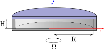
Figure 1: Rotor-stator geometry with rotating shroud. The set-up is characterised by the Reynolds number $Re={\Omega H^{2}}/{\nu}$ and an aspect ratio $\Gamma=R/H$ fixed in most of this article to 10.

2 Governing equations and numerical methods

The system consists of two coaxial disks of radius $R$, separated by a gap $H$. One of the disks, the rotor, rotates at a constant dimensional angular velocity $\Omega$, while the stator is at rest, see figure 1. We chose to non-dimensionalise all lengths by the gap $H$ and time using $(\Omega)^{-1}$. Assuming a constant kinematic viscosity $\nu$ for the fluid, two non-dimensional parameters characterise this system, namely the geometric aspect ratio $\Gamma=R/H$ and the (gap-based) Reynolds number $Re=\Omega H^{2}/\nu$.

2.1 Governing equations

The non-dimensional velocity $\mathbf{v}=(v_{r},v_{\theta},v_{z})$ and the non-dimensional pressure $\pi$ obey the incompressible Navier-Stokes equations (1 – 4). Throughout the whole paper we assume that the flow is strictly axisymmetric. We consider the Navier–Stokes equations in the cylindrical coordinate system $({\bm{e}}_{r},{\bm{e}_{\theta}},{\bm{e}_{z}})$ :

$$\frac{\partial v_{r}}{\partial t}+v_{r}\frac{\partial v_{r}}{\partial r}+v_{z}\frac{\partial v_{r}}{\partial z}-\frac{v^{2}_{\theta}}{r}=-\frac{\partial\pi}{\partial r}+\frac{1}{Re}(\frac{1}{r}\frac{\partial}{\partial r}(r\frac{\partial v_{r}}{\partial r})-\frac{v_{r}}{r^{2}}+\frac{\partial^{2}v_{r}}{\partial z^{2}})$$ (1)

$$\frac{\partial v_{\theta}}{\partial t}+v_{r}\frac{\partial v_{\theta}}{\partial r}+v_{z}\frac{\partial v_{\theta}}{\partial z}+\frac{v_{r}v_{\theta}}{r}=\frac{1}{Re}(\frac{1}{r}\frac{\partial}{\partial r}(r\frac{\partial v_{\theta}}{\partial r})-\frac{v_{\theta}}{r^{2}}+\frac{\partial^{2}v_{\theta}}{\partial z^{2}})$$ (2)

$$\frac{\partial v_{z}}{\partial t}+v_{r}\frac{\partial v_{z}}{\partial r}+v_{z}\frac{\partial v_{z}}{\partial z}=-\frac{\partial\pi}{\partial z}+\frac{1}{Re}(\frac{1}{r}\frac{\partial}{\partial r}(r\frac{\partial v_{z}}{\partial r})+\frac{\partial^{2}v_{z}}{\partial z^{2}})$$ (3)

$$\frac{1}{r}\frac{\partial(rv_{r})}{\partial r}+\frac{\partial v_{z}}{\partial z}=0,$$ (4)

The coupled system of partial differential equations is complemented with the no-slip boundary conditions expressed as (5) :

$$\begin{cases}{\bm{v}}=r{\bm{e}_{\theta}},&\text{at the rotor $(z=0)$}\\ {\bm{v}}=\Gamma{\bm{e}_{\theta}},&\text{at the shroud $(r=\Gamma)$}\\ {\bm{v}}={\bm{0}},&\text{on the stator $(z=1)$},\\ \end{cases}$$ (5)

resolution	$N_{r}$	$N_{z}$	type	DOF
R0	300	80	uniform	99 k
R1	600	160	uniform	390 k
R2	1024	192	non-uniform	796 k
R3	1536	288	non-uniform	1.8 m

Table 1: Mesh resolutions used in the study.

2.2 Discretisation

The continuous problem is discretised using a second order Finite Volume method on a staggered grid. The details of the discretisation as well as the staggered arrangement can be found in appendix A of Faugaret et al. (2022). Two types of mesh, uniform and non-uniform, are used. The non-uniform mesh is refined in the regions near the rotor, the stator and the rotating shroud. Details on the nonuniform mesh setup can be found in Gesla et al. (2023).

Details on the spatial discretisation used are given in Table 1. In both uniform and non-uniform cases, the number of pressure cells in the radial direction $r$ (resp. the axial direction $z$) is noted $N_{r}$ (resp. $N_{z}$). For the application of the boundary conditions a layer of ghost cells is added outside the physical domain.

2.3 Numerical methods

The nonlinear system of Eqs. (1 – 4) admits for all $Re$ a steady solution. Once the system is discretised, the solution of the large algebraic nonlinear system of equations is determined numerically using a Newton-Raphson algorithm (see e.g. appendix B in Faugaret et al. (2022)). The $O(4N_{r}N_{z})$ unknowns are the velocity and pressure values at each discretisation point. Due to the presence of the thin boundary layers close to each disk, the set of equations resulting from the discretisation of the continuous system is in general poorly conditioned. Sparse direct solvers will be therefore preferred over the iterative solvers for solving the linear systems in each Newton-Raphson iteration.

A technical remark concerning the geometry can be made at this point : at the junction between the rotating shroud and the stationary disc, the sudden change in $u_{\theta}$ imposed in the boundary condition induces a discontinuity of the velocity field in the $(r,z)=(\Gamma,1)$ corner. This singularity can have an impact on the accuracy of the numerical solutions. In order to avoid singular boundary conditions and the well-known associated Gibbs phenomenon, several teams using pseudospectral solvers (Serre et al., 2004; Lopez et al., 2009) proposed to smooth out the discontinuous boundary condition between the stator and the shroud. Whenever Finite Volume discretisation is used the singular corner does not degrade the second order of spatial accuracy of the scheme, as demonstrated in Gesla et al. (2023).

The linear stability of the base flow is evaluated using the Arnoldi method based on a well-validated ARPACK package (Lehoucq et al., 1998). A generalised eigenvalue problem can be constructed using the Jacobian matrix used in the procedure of finding the base flow stemming from linearisation of the governing equations around a base flow (section 4). For a generalised eigenvalue problem

$$\bm{A}\bm{w}=\lambda\bm{B}\bm{w},$$ (6)

the shift-and-invert method finds a subset of eigenvalues closest to a complex shift $s$ through repeated Arnoldi iteration:

$$\nu\bm{w}=\left(\bm{A}-s\bm{B}\right)^{-1}\bm{B}\bm{w}$$ (7)

where the original eigenvalues $\lambda$ can be retrieved with:

$$\nu=\frac{1}{\lambda-s}$$ (8)

The time integration of the governing equations uses a prediction-projection algorithm in the rotational pressure correction formulation as described in Guermond et al. (2006). The prediction step combines a Backwards Differentiation Formula 2 (BDF2) scheme for the diffusion terms and an explicit treatment of the convective terms, resulting in a Helmholtz problem for each velocity component increment. These Helmholtz problems are solved using an alternating-direction implicit (ADI) method in incremental form which preserves the second order accuracy in time. In the projection step the velocity field is projected onto the space of divergence-free fields by solving a Poisson equation for the pressure. This Poisson equation is solved using a direct sparse solver. Once the base flow solution is found, the time-stepping code can be adapted to evolve the perturbation to the base flow rather than the full velocity field itself, at the expense of a triple evaluation of the convective terms.

3 Base flow

The base flow is the steady axisymmetric velocity field ${\bm{U}_{b}}$ solution to the governing equations (1-4) compatible with the boundary conditions (5). It is associated with a pressure field $p_{b}$ defined up to an additive constant. It consists, for high enough $Re$, of two boundary layers, one on each disk, and a core region. Fluid is forced into circulation around the cavity by the rotation of the bottom disc. It is advected towards the rotating shroud and returns towards the axis along the stationary disk. In figure 2(left) isocontours of $u_{\theta}$ fields are plotted for increasing $Re$. The meridional recirculation plane is shown using meridional streamlines in figure 2(right). Streamfunction $\psi(r,z)$ is defined implicitly by $v_{r}=\frac{1}{r}\frac{\partial\psi}{\partial z}$ and $v_{z}=-\frac{1}{r}\frac{\partial\psi}{\partial r}$. For high enough $Re$ the core region between the boundary layers appears almost independent of $z$.

For the case $\Gamma=10$, a linear instability of the base flow in the axisymmetric configuration was found for $Re\approx 3000$, due to the destabilisation of a wavepacket of counter-rotating circular rolls in the Bödewadt layer at $r\approx 2$ for $Re\approx 3000$ (Daube & Le Quéré, 2002). This result was recently confirmed quantitatively by Gesla et al. (2023). This threshold for axisymmetric instability is one order of magnitude larger than the experimental threshold of $Re\approx 200$ reported e.g. in Gauthier (1998).

The base flow being linearly stable in the $Re$-interval of interest for this study, it can in principle be found by asymptotic time integration. Nevertheless, for accuracy purposes and in order to avoid to avoid strong transient growth effects (Daube & Le Quéré, 2002; Gesla et al., 2023) it is safest to converge the base flow using the dedicated Newton-Raphson solver. In the rest of the paper, once the base flow is known, we deal exclusively with axisymmetric perturbation ${\bm{u}}(r,z,t)$ to the base flow solutions, i.e. ${\bm{u}}={\bm{v}}-{\bm{U}_{b}}$ and $p=\pi-p_{b}$, the equations for which can be deduced directly from the governing equations by subtraction. The associated boundary conditions are homogeneous of Dirichlet type, i.e. ${\bm{u}}=0$ at all walls. At the axis ($r=0$) $u_{r}$ and $u_{\theta}$ vanish while $u_{z}$ verifies a Neumann condition.

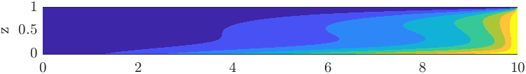
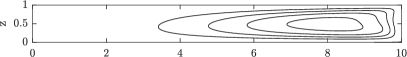
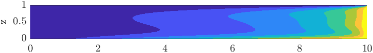
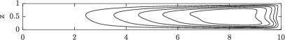
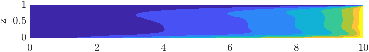
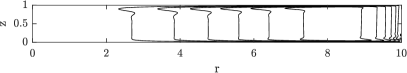
Figure 2: Axisymmetric base flow solution for $\Gamma=10$. Visualisations in a meridian section. From top to bottom : Re=70, 150, 250, 3000. Left: azimuthal velocity $u_{\theta}(r,z)$. The colormap divides the interval (0,10) in 8 equal subintervals. Right: streamfunction $\psi(r,z)$. Plotted values : $\psi_{Re=70}=1,(1),4$. $\psi_{Re=150}=0.5,(0.5),2.5$. $\psi_{Re=250}=0.5,(0.5),2$. $\psi_{Re=3000}=0.1,(0.1),0.6$. $\psi=0$ corresponds to the wall. Numerical resolution R1.

4 Linear response to forcing

4.1 Optimal response theory

In this subsection the linear response of the flow to the forcing is analysed using optimal response theory. Following Cerqueira & Sipp (2014) we conduct the input/output analysis and show that the optimal response of the flow is for most relevant values of $Re$ in the shape of circular rolls, and that associated with high levels of optimal gain. The nonlinear system of equations (1 – 4) can be linearised around the base flow when perturbation velocities are small enough. If a forcing field ${\bm{f}}$ is introduced, the resulting system for the perturbation field $({\bm{u}},p)$ can be rewritten

$$\frac{\partial{\bm{u}}}{\partial t}+({\bm{U}_{b}}\cdot{\bm{\nabla}}){\bm{u}}+({\bm{u}}\cdot{\bm{\nabla}}){\bm{U}_{b}}=-{\bm{\nabla}}p+\frac{1}{Re}{\bm{\nabla}}^{2}{\bm{u}}+{\bm{f}}\>,$$ (9)

$${\bm{\nabla}}\cdot{\bm{u}}=0\>.$$ (10)

The coupled system in (9)-(10) is linear in ${\bm{u}}$, $p$ and also ${\bm{f}}$, which suggests to use the resolvent formalism. The theory by Trefethen & Embree (2005) forms the ideal framework except that the original linear system needs be rewritten in a form $\partial{\bm{z}}/\partial t={\bm{L}\bm{z}}+{\bm{f}_{z}}(t)$, where the unknown field ${\bm{z}}$, a linear operator ${\bm{L}}$ and a forcing ${\bm{f}_{z}}(t)$ need to be specified. We introduce the new variable $\mathbf{q}=(u_{r},u_{\theta},u_{z},p)$ which contains the values of the fields $u_{r}$,$u_{\theta}$, $u_{z}$ and $p$ at all the points of the discretised domain. The size of $\mathbf{q}$ is $O(4N_{r}N_{z})$. We also introduce the rectangular prolongation operator ${\bm{P}}$ of size $O(4N_{r}N_{z}\times 3N_{r}N_{z})$ which maps ${\bm{u}}$ into ${\bm{q}}$, so that $\mathbf{P}^{T}\mathbf{q}=\mathbf{u}$ with the property $\mathbf{P}^{T}\mathbf{P}=\mathbf{I}$, see e.g. Jin et al. (2021). The linear system (9– 10) can then be rewritten into the new form

$$\mathbf{B}\frac{\partial\mathbf{q}}{\partial t}=\mathbf{A}\mathbf{q}+\mathbf{P}{\mathbf{f}},$$ (11)

where $\mathbf{B}=\mathbf{P}\mathbf{P}^{T}$. After a Fourier transform in time, each Fourier component $\hat{\mathbf{q}}$ of $\mathbf{q}$ satisfies

$$\left(i\omega\mathbf{B}-\mathbf{A}\right)\hat{\mathbf{q}}=\mathbf{P}\hat{\mathbf{f}}\>,$$ (12)

resulting in the Fourier components $\mathbf{\hat{u}}$ of the velocity field $\mathbf{u}$ as the action of a matrix $\mathbf{R}$ on the forcing $\mathbf{\hat{f}}$ :

$$\hat{\mathbf{u}}=\mathbf{R}\hat{\mathbf{f}}$$ (13)

where

$$\mathbf{R}=\mathbf{P}^{T}\left(i\omega\mathbf{B}-\mathbf{A}\right)^{-1}\mathbf{P}\\$$ (14)

is the resolvent operator associated with the (real) angular frequency $\omega$.

An optimal gain can be evaluated by identifying an optimal forcing for a suitable norm of the resolvent $\mathbf{R}$. A positive symmetric linear operator $\mathbf{Q}\neq\mathbf{I}$, associated with the cylindrical coordinate system, can be used to define the inner product

$$<\mathbf{u},\mathbf{v}>_{\mathbf{Q}}=\mathbf{u}^{*}\mathbf{Q}\mathbf{v}=\int_{0}^{1}\int_{0}^{\Gamma}(u_{r}^{*}v_{r}+u_{\theta}^{*}v_{\theta}+u_{z}^{*}v_{z})rdrdz,$$ (15)

where the asterisk denotes complex conjugate. The associated vector norm is defined by

$$||\mathbf{u}||_{\mathbf{Q}}=\sqrt{\mathbf{u}^{*}\mathbf{Z}^{T}\mathbf{Z}\mathbf{u}}=||\mathbf{Z}\mathbf{u}||_{2},$$ (16)

where $\mathbf{Q}=\mathbf{Z}^{T}\mathbf{Z}$. $\mathbf{Q}$ can be also used to define the following norm for the resolvent operator

$$||\mathbf{R}||_{\mathbf{Q}}=||\mathbf{Z}\mathbf{R}\mathbf{Z}^{-1}||_{2}=\sigma_{1}(\mathbf{Z}\mathbf{R}\mathbf{Z}^{-1}),$$ (17)

where $\sigma_{1}$ denotes the largest singular value in the SVD decomposition. Note that finding the largest singular value of $\mathbf{ZRZ^{-1}}$ is equivalent to finding the largest eigenvalue of the eigenvalue problem (Cerqueira & Sipp, 2014):

$$\mathbf{R}^{*}\mathbf{Q}\mathbf{R}\mathbf{\hat{f}}=\lambda\mathbf{Q}\mathbf{\hat{f}}$$ (18)

where

$$G=\lambda=\sigma_{1}^{2}=\frac{\mathbf{\hat{u}}^{*}\mathbf{Q}\mathbf{\hat{u}}}{\mathbf{\hat{f}}^{*}\mathbf{Q}\mathbf{\hat{f}}}$$ (19)

is interpreted as the optimal energy gain.

4.2 Optimal response : results

For a range of angular frequencies $\omega$ the eigenvalue problem (18) is solved numerically in MATLAB with the eigs() function. The resulting eigenvalue $G=\sigma_{1}^{2}$ from Eq. 19 is plotted in figure 3 (left) as a function of the (real) angular frequency of the forcing. The optimal value $\sigma_{max}^{2}$ over all angular frequencies obtained for various values of $Re$ are compared in figure 3(right), with the case $\omega=0$ singled out. The optimal value of $G$ gain over all $\omega$’s, i.e. the optimal gain, is also listed in the table 2 together with the values obtained with different mesh resolutions.

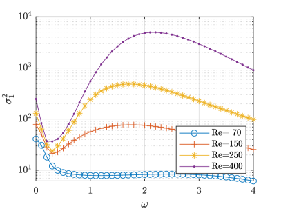
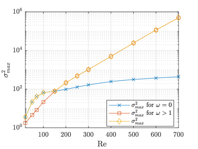
Figure 3: Optimal response for bulk-based forcing. Left: optimal energy gain as a function of forcing angular frequency $\omega$, given by the largest singular value of the resolvent operator (14). Right: optimal gain across all $\omega$’s as a function of $Re$. Numerical resolution R0.

Re	$\sigma_{max}^{2}$(R0)	$\sigma_{max}^{2}$(R1)	$\sigma_{max}^{2}$(R2)	$\sigma_{max}^{2}$(R3)	$\omega$
20	$3.61\times 10^{0}$				0.0
50	$2.20\times 10^{1}$				0.0
70	$4.10\times 10^{1}$	$4.10\times 10^{1}$			0.0
100	$6.59\times 10^{1}$				0.0
150	$7.85\times 10^{1}$	$7.86\times 10^{1}$	$7.87\times 10^{1}$		0.0
200	$2.14\times 10^{2}$				1.6
250	$4.84\times 10^{2}$	$4.94\times 10^{2}$	$4.90\times 10^{2}$		1.7
300	$1.04\times 10^{3}$				1.9
400	$4.95\times 10^{3}$	$5.50\times 10^{3}$	$5.47\times 10^{3}$		2.2
500	$2.45\times 10^{4}$				2.4
600	$1.15\times 10^{5}$				2.6
700	$4.97\times 10^{5}$	$7.62\times 10^{5}$	$7.96\times 10^{5}$	$8.38\times 10^{5}$	2.9
1800		$7.10\times 10^{11}$	$1.29\times 10^{12}$	$1.50\times 10^{12}$	4.3
3000		$2.08\times 10^{16}$	$1.28\times 10^{17}$	$1.66\times 10^{17}$	5.4

Table 2: Optimal forcing gain. The last column shows the optimal angular frequency $\omega$ associated with the largest energy gain (the computations are performed with a step of 0.1 in angular frequency). Four mesh resolutions (see table 1) are used to find the optimal gain value. While for $Re\approx 250$ results can be considered as satisfactory for resolution R1, increased resolution is needed for larger $Re$. This is due to increasingly thin boundary layers required to resolve the optimal forcing mode.

	forcing	response
Re = 70 $\omega=0$
Re = 150 $\omega=0$
Re = 1800 $\omega=0$
Re = 3000 $\omega=0$

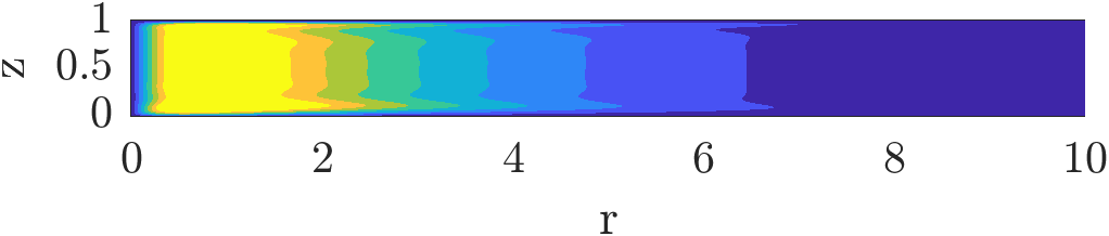
Figure 4: Azimuthal perturbation velocity $u_{\theta}(r,z)$ for optimal forcing and optimal response for vanishing forcing frequency $\omega=0$. For Re=70 and 150 the optimal forcing at $\omega=0$ is also optimal across all $\omega$’s. The colormap spans 8 equal subintervals of $[0,0.5]$. Both optimal forcing and response are normalised such that $||\mathbf{\hat{f}}||_{\mathbf{Q}}=||\mathbf{\hat{u}}||_{\mathbf{Q}}=1$.

For low $Re<150$ the optimally amplified frequency is always $\omega=0$ . This corresponds to a steady forcing $f$ in the equations (1 – 4). Forcing a given flow at $\omega=0$ can be interpreted in different complementary ways. It can first be understood as the smooth $\omega\rightarrow 0$ limit of a given harmonic forcing at frequency $\omega$. It can also be understood, in the unforced problem, as the steady streaming component associated with the nonlinear self-interaction of arbitrary oscillatory perturbations (see e.g. Mantič-Lugo et al. (2014)). In both cases the optimal response at $\omega=0$ is interpreted as an optimal steady mean flow correction, which justifies the special focus on $\omega=0$. As seen in figure 4 the most amplified steady forcing is always localised in the region near the axis. For $Re>1800$ it inherits the characteristics of the base flow in the sense that it is composed of two boundary layers and invariant core in between.

	forcing	response
$u_{r}$
$u_{\theta}$
$u_{z}$

Figure 5: Optimal forcing and response for Re=250. From top to bottom : perturbation velocity components $u_{r}$, $u_{\theta}$ and $u_{z}$ for the optimal angular frequency $\omega=1.7$. The colormap spans 8 equal subintervals of (-0.15 0.15) for the optimal forcing, and (-0.6 0.6) for the optimal response plots. The optimal forcing and response are normalised such that $||\mathbf{\hat{u}}||_{\mathbf{Q}}=||\mathbf{\hat{f}}||_{\mathbf{Q}}=1$.

For $Re\approx 150$ the optimally forced structures change radically as unsteady ($\omega\neq 0$) forcing takes over steady forcing. This is clearly seen in figure 3(right) where for $Re\gtrsim 150$ nonzero forcing frequencies $\omega$ start to dominate the optimal gain curve. The structure of the associated optimal forcing lies entirely within the Bödewadt layer, see figure 5 which focuses on $\omega\approx 1.7$ close to the optimal angular frequency (see Table 2). For all velocity components these structures are tilted by the mean shear into the streamwise direction. While the amplitude of optimal forcing is similar in the three spatial components the corresponding optimal response may differ from component to component (Jovanović & Bamieh, 2005), and in the present geometry it is clearly dominated by the azimuthal component. The signature of the circular rolls can be also seen in the azimuthal response although the corresponding structures should more realistically be labelled as azimuthal streaks. Their position ($r\approx 4-6$) and the corresponding $Re$ are perfectly consistent with experimental observations. Most importantly, and this constitutes one of the main findings of the current work, the optimal response is in the shape of circular rolls in the Bödewadt layer.

The evolution of the optimally forced structure is now described as $Re$ increases beyond 250. It is first noted that, as shown in figure 3 (right), the optimal gain $G_{opt}(Re)$ grows exponentially with $Re$. We note that the experimental study of Gauthier et al. (1999), performed for $\Gamma\approx 20$, has suggested a supercritical bifurcation as the origin of the observed rolls. Our observations do not corroborate this hypothesis since the angular frequency content of the response features that a continuum of frequencies can be excited externally, at odds with the dominant frequency stemming from a Hopf bifurcation. Moreover, the steep exponential increase of $G(Re)$ reported above might be responsible, in experimental conditions where external forcing stays uncontrolled, for the apparent bifurcating behaviour where the amplitude of the response increases rapidly with $Re$. As $Re$ continues to increase, as shown in figure 6 the optimal forcing evolves with $Re$ from a wide support within the Bödewadt layer to thinner structures in both the Bödewadt and the shrouding wall, and even for $Re=3000$ also in the Ekman layer. For such high $Re$ values the respective supports of the forcing and the response are almost disjoint.

The results above unambiguously point towards an unsteady response in the shape of circular rolls for all $Re\gtrsim 150$. We emphasize that the crossing of the gain curves for $\omega=0$ and $\neq 0$ in figure 3(right) does not define a threshold value for $Re$ because, as for any linear receptivity mechanism, the response depends linearly on the spectral content of the forcing history. Defining a threshold value for $Re$ is demanding because it is highly dependent on the amplitude levels that an experimentalist can detect in practice. By focusing on the value of the optimal gain ($G=4.9\times 10^{2}$) at $Re=250$ the following hand-wavy evaluation can be made. Any parasite vibration present in the experiment projected on the orthogonal basis of the optimal modes will have a nonzero component that will be optimally forced. If the amplitude of this component is, say, of order $O(10^{-2})$ it will be amplified by the linear mechanism by $\sqrt{G}\approx 20$ to yield an $O(10^{-1})$ response, which can be detected in experiments.

	forcing	response
Re = 150 $\omega=1.8$
Re = 250 $\omega=1.7$
Re = 1800 $\omega=4.3$
Re = 3000 $\omega=5.4$

Figure 6: Azimuthal perturbation velocity $u_{\theta}(r,z)$ for the optimal forcing and response for $\omega\neq 0$. For Re=250, 1800 and 3000 the optimal forcing is also optimal across all $\omega$’s. The colormap spans 8 equal subintervals of (-0.15 0.15) for the optimal forcing and (-0.6 0.6) for the optimal response.

4.3 Boundary forcing

While the previous section offers an elegant formal manner to explain the circular rolls from (linear) optimality arguments, we note that at the experimentally relevant values of $Re$, the optimal forcing protocol corresponds to a force field that needs to be applied to the flow away from the solid boundaries. Set-up imperfections are expected to induce forcing at the boundaries rather than away from them. For this reason, it is unlikely that the observed linear response corresponds to truly optimal forcing, and it might be more relevant to concentrate on sub-optimal forcing. Instead, we consider a forcing protocol which without being energetically optimal affects directly the flow through unsteady motion of the boundaries (and is hence not a suboptimal from the previous bulk-based optimisation). Modulations of the instantaneous (dimensional) angular velocity are considered in the form $\Omega(t)=\Omega_{0}(1+A\ \varepsilon(t))$, where $\varepsilon(t)$ represents a normalised unsteady forcing and $A\geq 0$ is a measure of its amplitude. This is similar to Lopez et al. (2009), Poncet et al. (2009) and Do et al. (2010), except that $\varepsilon(t)$ is not monochromatic. The Reynolds number, now based on $\Omega_{0}$ rather than $\Omega$ (which depends on time), remains by definition unaffected by the value of $A$.

4.3.1 Time integration

The time modulation is simulated in practice by updating, at the end of each timestep after the prediction-projection step, the value of $v_{\theta}$ imposed on the shroud and the rotor as

$$v_{\theta}(r,t)=r(1+A\ \varepsilon(t))$$ (20)

The modulation $\varepsilon(t)$ can be chosen in many ways. For most of this study, it is chosen as a Gaussian white noise of zero mean and standard deviation 1. $A$, which multiplies the white noise signal, is therefore the root mean square (rms) value of the forcing. All simulations are initiated with a zero perturbation field.

Figure 7: Nonlinear time integration in the presence of white noise forcing at the $r=\Gamma$ boundary with amplitude $A=10^{-2}$. Snapshots of the azimuthal perturbation velocity $u_{\theta}(r,z)$. From top to bottom: $Re=70,\ 150,\ 250,\ 400$. A wavetrain of circular rolls is seen for $Re>250$.

Figure 7 shows representative azimuthal velocity snapshots obtained from nonlinear time integration of the forced flow. As will be clear later in section 6, for the aspect ratio $\Gamma=10$ and $Re<300$ nonlinearity plays a negligible role and the observations are independent of whether the time integration is linear or nonlinear. This is why those results are discussed in the context of linearly optimal results. The response to the unsteady white noise forcing is localised, for low $Re\approx 70$, next to the rotor and the shroud. For $Re\gtrsim 150$ and beyond, wavetrains of increasingly smaller circular rolls form inside the Bödewadt layer, as is visible for $Re=250$ and $Re=400$.

Interestingly, the response to boundary forcing is similar to the response to the optimal forcing in the sense that the response consists also of wavetrains of circular rolls located inside the Bödewadt layer. Due to the wide frequency content this response is however more widespread than in the case of optimal forcing (e.g. for $Re=250$ the wavetrain is detected for $r\in(2,7)$). A pronounced response near the rotor and especially the shroud is also seen, as a signature of the imposed forcing.

4.3.2 Resolvent approach to boundary forcing

The connection between the linearised time integration and the resolvent approach from (12) is the Fourier transform of the linearised governing equations. Selecting the additive forcing term $\mathbf{\hat{f}}$ corresponding to the forcing protocol of (20), and then solving (13) for $\mathbf{\hat{u}}$ will therefore yield directly the Fourier transform of the response. It can be in turn compared against the Fourier transform of the probe signals extracted from linearised time integration. The same analogy has been exploited by Cerqueira & Sipp (2014) in order to validate their input/output analysis. In our case, beyond immediate validation, this comparison is useful as it draws a link between boundary forcing (although based on linear time integration rather than the nonlinear integration allowing for spectral mixing) and the inherently bulk-based resolvent approach.

We therefore select a specific, non-optimal forcing term $\mathbf{P\hat{f}}$ corresponding to the Fourier transform of the boundary forcing (20). Solving (12) with prescribed $\mathbf{P\hat{f}}$ yields $\mathbf{P\hat{u}}$, the real part of which is plotted in figure 8. The (squared) $\mathbf{Q}$-norm of $\mathbf{\hat{u}}$ is shown in the same figure. Due to the forcing being suboptimal, its dependence on $\omega$ differs from the gain curve in figure 3 (left). Again, starting with $Re=250$ a hump visible in figure 8(left) around $\omega=2$ marks the preferred response of the flow in the shape of rolls.

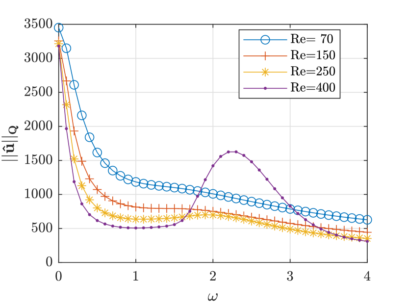
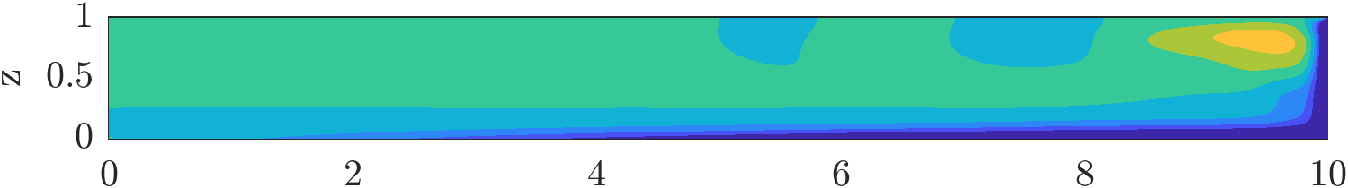
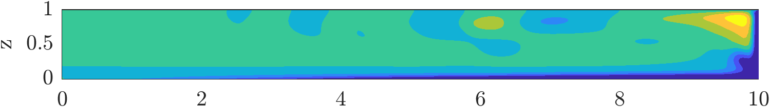
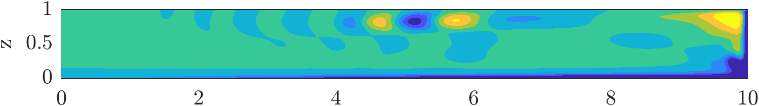
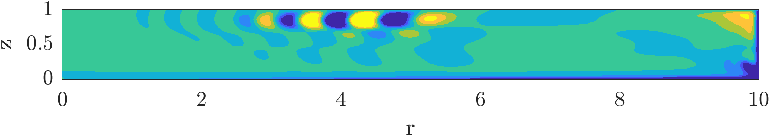
Figure 8: Response to the boundary forcing obtained by the resolvent approach in section 4.3.2. Left: $\mathbf{Q}$-norm (squared) of the velocity response. Right, from top to bottom: real part of $\hat{u}_{\theta}(r,z)$ for $\omega=2$ for $Re=\ 70,\ 150,\ 250,\ 400$. The $\mathbf{\hat{u}}$ response is normalised so that $||\mathbf{\hat{u}}||_{\mathbf{Q}}=1$. Colormap spans $-0.3,(0.075),0.3$.

More insight into the preferred response frequencies of the flow is possible through the analysis of the probe signals extracted from linear time integration. The raw signals, corresponding to four radial positions $r=1,3,5,7$ along the Bödewadt layer, are shown in figure 9(left). The forcing is again white in time with equal amplitude for each frequency. The Fourier transform of the probe signal confirms, as already visible from the fields in figure 7 and 8, that the strength of the response to boundary forcing depends on the radial position. The radially inwards flow in the Bödewadt layer suggests that the distance to the shrouding wall, and therefore the varying thickness of the boundary layer, are the physically meaningful variables to explain this dependency, as also suggested by Gauthier et al. (1999) (we will however stick to the variable $r$ for commodity). The preferred response frequency evolves also with the radial position. It is close to $\omega=0$ for the probe at $r=1$, but close to $\omega=3$ for the probe $r=7$. The Fourier amplitude can be directly compared to the pointwise amplitude of $\mathbf{\hat{u}}$, as mentioned earlier. The convincing overlap of both data (see figure 9(right)) demonstrates the equivalence between the linear time integration and the direct resolvent solve based on (13).

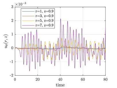
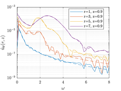
Figure 9: Response to boundary forcing by Gaussian white noise with $A=10^{-2}$, Re=200. Left: time series of perturbation velocity $u_{\theta}$ obtained from time integration for different probes at varying $r$ inside the Bödewadt layer z=0.9. Right: comparison between the time integration and the resolvent approach to boundary forcing in frequency space. Fourier amplitude spectrum of these time series (solid lines) versus ${|\hat{u}_{\theta}|}$ associated with boundary forcing, computed from resolvent analysis (dashed lines) and evaluated at the same spatial positions. Numerical parameters $dt=4\cdot 10^{-3}$, $nt=20\ 000$, $d\omega=0.157$, $\omega_{Nyquist}=785$ corresponding to the timestep, number of timesteps, sampling angular frequency and Nyquist angular frequency respectively. Only the later half of the signal was used for the calculation of the Fourier transform ($40<t<80$).

4.4 Computation of the pseudospectrum

A fundamental tool in the analysis of non-normal systems is the pseudospectrum, which is a generalisation of the concept of (eigen)spectrum. Recall that the spectrum of the linearised system $\dot{{\bm{u}}}=\mathbf{L}{\bm{u}}$ is the (complex) set of eigenvalues of the associated linear operator. If a complex number $\omega$ belongs to the spectrum $\sigma$, the resolvent $(i\omega\mathbf{I}-\mathbf{L})^{-1}$ (or expressed in the present case by (14)) is undefined, whereas it is continuous and smooth as a function of $\omega$ in the immediate neighbourhood of its pole at $i\omega$. Following Trefethen & Embree (2005) the $\varepsilon$-pseudospectrum $\sigma_{\varepsilon}$ is defined as the complex set where the norm of the resolvent operator exceeds a given value $\varepsilon^{-1}$, with $\varepsilon$ a potentially small real number :

$$\sigma_{\varepsilon}=\{\omega\in\mathbb{C},||\mathbf{R}||_{\mathbf{Q}}>\varepsilon^{-1}\}$$ (21)

It includes the point spectrum and can be seen as its generalisation. In the current work, it is mainly used as an indicator of the strong non-normality of the underlying linearized operator. Owing to the definition 21, the cut of the pseudospectrum through the real axis directly yields the gain curves plotted in figure 3. The pseudospectrum is computed in each point, analogously to the optimal gains described in section 4.1, except that $\omega$ is allowed to be complex. Note that such computations rely on the shift-and-invert algorithm itself dependent on a purely imaginary shift parameter $s$. Contours of the pseudospectrum are reported in figure 10. As expected for a strongly non-normal operator, the isocontours of $\sigma_{\varepsilon}$ do not form concentric circles around the eigenvalues yet the contours encircle more than one eigenvalue. Still, very close locally to a given eigenvalue, the isocontours found for $Re=200$ form closed loops around specific eigenvalues, as can be seen in the top right panel in figure 10. Upon increasing $Re$, the non-normality of the linearized operator increases and the background level in the pseudospectrum grows, as shown in figure 10.

Another useful information from pseudospectra is the sensitivity of an eigenvalue to arbitrary perturbations of the operator $\mathbf{L}$ (Cerqueira & Sipp, 2014; Brynjell-Rahkola et al., 2017). As shown in chapter 28 of Trefethen & Embree (2005) for a convection-diffusion operator, high levels of non-normality typically cause iterative Arnoldi methods to converge to false eigenvalues. This is easily verified by comparing the effect of different shift values $\sigma$ in the shift-inverse Arnoldi iteration. Here, as in Cerqueira & Sipp (2014), very large level of pseudospectral contours, typically above 11, prevent ARPACK from accurately converging all the eigenvalues. This algorithmic sensibility is not only a numerical convergence problem, it also highlights a physically ambiguous situation. Individual eigenvalues, when they are not robust, do not yield a specific contribution to the dynamics. In particular the associated eigenfrequencies are not resonant, and a large response to forcing is obtained even for forcing frequencies far from the eigenfrequencies (Trefethen et al., 1993). This is associated with the presence of a large hump (rather than narrow peaks) in the gain curve. In such a case, frequent in shear flows such as jets or boundary layers, one speaks of pseudo-resonance, see e.g. Garnaud et al. (2013). Non-robust eigenvalues are easily spotted as soon as their location in the complex plane depends on the shift $\sigma$ chosen by the user, see figure 10(bottom right). Conversely, the most unstable eigenvalue $\lambda_{r}=0.011,\ \lambda_{i}=1.95$ at $Re=3000$ in figure 10 can be trusted, and the growth rate $\lambda_{r}$ predicted by the computation of eigenvalues will correspond to the growth rate of instability upon time linearized integration.

Finally, the pseudospectra can also be post-processed to extract a lower bound on the maximal transient growth associated with given initial perturbations. Following Chap. 14 in Trefethen & Embree (2005), the Kreiss constant is the lower bound of the maximal growth of the initial perturbation and is defined by:

$$\mathcal{K}=\sup_{\varepsilon>0}\frac{\alpha_{\varepsilon}}{\varepsilon}$$ (22)

where $\alpha_{\varepsilon}$ is the pseudospectral abscissa (the maximal real part of the $\varepsilon$ contour in the complex plane). Computation of $\mathcal{K}$ for pseudospectra in figure 10 gives $\mathcal{K}_{Re=200}=1.4\times 10^{3}$ and $\mathcal{K}_{Re=3000}=2.2\times 10^{8}$, suggesting very large growth potential, as demonstrated by Daube & Le Quéré (2002) and Gesla et al. (2023) for the same set-up.

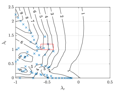
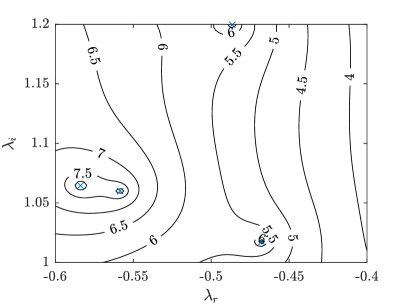
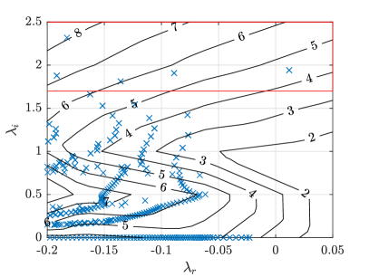
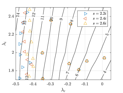
Figure 10: Pseudospectrum levels $log_{10}||\mathbf{R}||_{\mathbf{Q}}$ in the complex plane where $\lambda_{r}$ and $\lambda_{i}$ are the real and imaginary part of the complex number $i\omega$. Top: $Re=200$, bottom: $Re=3000$. The right plot corresponds to the red inset in the left plot, where three different values of the shift $s$ in the shift-and-invert algorithm have been used.

5 Experimental comparison

In this section, an effort is made to reproduce the experimental conditions where axisymmetric rolls were reported. A detailed comparison with the literature results can be challenging because of the many different configurations of the rotor-stator system reported in the literature. Apart from the value of the aspect ratio $\Gamma$, special attention has to be given to whether or not the shroud is rotating and whether the cavity extends or not to the axis. The latter case corresponds to the presence of a hub. Relevant experimental studies of the rotor-stator configuration at moderate aspect ratio $\Gamma$ (from around 5 to around 20) are listed below :

1. Gauthier (1998), with a rotating shroud and no hub, reports circular rolls at $Re\approx 70$ for $\Gamma=20.9$ and at $Re\approx 180$ for $\Gamma=10$

2. Schouveiler et al. (2001) with a fixed shroud and no hub, reports circular rolls for a range of $\Gamma$, in particular at $Re\approx 160$ (deduced from figure 3 (Schouveiler et al., 2001) for $\Gamma=10$)

3. Poncet et al. (2009) with a fixed shroud and a rotating hub, reports circular rolls at $Re=160$ for $\Gamma=8.8$

Numerical studies do not report sustained circular rolls in the absence of external forcing, at the exception of Daube & Le Quéré (2002) who considered larger $Re$ values.

We focus specifically on the article by Schouveiler et al. (2001) and the corresponding parameters. The aspect ratio is hence temporary set to $\Gamma=8.75$, the shroud is fixed and the range of values of $Re$ $(0:300)$ is selected. Unsteady nonlinear simulations with boundary forcing are performed with three different forcing protocols. The main difficulties in comparing numerics to experiments are the fact that i) the amplitude of the forcing is unknown ii) the temporal frequency spectrum of the forcing is often unknown. Three qualitatively different types of forcing have hence been considered here : monochromatic forcing, analogously to Do et al. (2010), with specific forcing frequency $\omega=1$, harmonic forcing where only harmonics of $\omega=1$ are considered, and eventually white noise forcing. In the case of harmonic forcing all the temporally resolvable harmonics of the disc angular frequency are forced with equal amplitude. This type of forcing is especially relevant to the experimental comparison : as shown in both Gauthier et al. (1999) and Faugaret (2020), the main spurious perturbations present in the experimental set-up are the disc harmonics. The studies of the forced regimes focused mostly on monochromatic forcing (Gauthier et al., 1999; Lopez et al., 2009; Do et al., 2010).

For these three forcing protocols an $r$-dependent observable needs to be monitored for all times. We select the observable $E(r,t)$ defined as

$$E(r,t)=\int_{\delta}^{1}((u_{r})^{2}+(u_{\theta})^{2}+(u_{z})^{2})\ dz,$$ (23)

where $\delta=0.2$ (in units of $H$) corresponds to integrating over 4/5 of the interdisc spacing (thereby excluding the parallel boundary layer along the rotor). This parameter $\delta=0.2$ is preferred over $\delta=0$ for the clarity of the resulting space-time diagrams. The results for the three type of forcing are presented in figure 11. All figures are accompanied by a snapshot of the same energy $E(r,t)$ at arbitrary time, seen from above in order to emphasize the visual comparison with experimental photographs. The three types of forcing all lead to wavetrains of circular rolls with $E$ locally stronger in the interval $0.34\leq r\leq 0.6$. The rolls reaching closest to the axis correspond to monochromatic forcing, while the front seems to remain further from the axis when the spectral content of the forcing is richer. The radial velocity of the rolls is always negative (oriented towards the axis) and can be estimated directly from the space-time diagrams. Even in the monochromatic case, their velocity is not constant and it depends on $r$ : since the Bödewadt layer thickens as the perturbations migrate towards the axis where the radial velocity vanishes, the phase velocity of the rolls has to decrease, until the rolls can no longer sustain. The space-time diagram for the monochromatic case, qualitatively similar to Fig. 11 in Do et al. (2010), illustrates this point particularly well. In the harmonic case, the coexistence of different frequencies leads to different radial velocities being possible at a given radius. The dynamics becomes more complex since rolls can now travel at different velocities, leading to consecutive rolls merging or splitting. The pattern shown in Fig. 11 (middle), which shows periodic pairing and merging near $r\approx 0.75$ resembles in particular the experimental pattern shown in Figure 6 in Ref. Schouveiler et al. (2001) at the same value of $Re$. As for the white noise forcing protocol, pairing and merging events appears more intermittently admits otherwise periodic roll propagation.

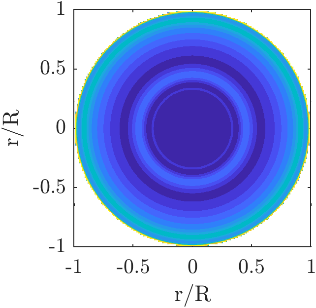
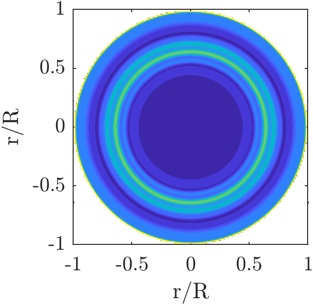
Figure 11: Energy integral $E(r,t)$ at Re=225, $\Gamma=8.75$. Time is non-dimensionalised by the disc rotation period. An initial transient was neglected. Excited rolls travel inwards with a radial phase speed depending on the radius. Top: mono-frequency forcing at angular frequency $\omega=1$. No merging and pairing of the rolls is observed. Middle: harmonic frequency $\omega=1,\ 2,\ 3,...$ forcing. Pairing and merging of the rolls are observed here. Rolls merge because the phase speed depends on the radial position and the roll frequency $\omega$. Bottom: white noise forcing. Complex roll dynamics is observed due to all frequencies being excited by the forcing.

The perfect agreement of the localisation of the rolls and the corresponding spacetime diagram with the experimental results of Schouveiler et al. (2001) both reinforce the interpretation of circular rolls as the preferred response of the system to external forcing.

6 Nonlinear receptivity

Receptivity to external disturbances in fluid flows is traditionally investigated using the linear toolbox of resolvent analysis, which is usually justified by the small perturbation velocities at play. This has the huge advantage that the responses to individual frequencies can be used as a basis to describe the global response to arbitrary forcing. Extensions of this formalism to finite-amplitude perturbations lead to new mathematical difficulties. Early efforts have focused on generalising the parabolised suitability equations (Bertolotti et al., 1992; Herbert, 1997), which unfortunately is not an option for recirculating flows. A recent attempt to add nonlinear triadic interactions to the resolvent formalism was recently proposed by Rigas et al. (2021) for boundary layer flow. For the rotor-stator flow the importance of nonlinear interactions in the dynamics of the circular rolls was already pointed out by Do et al. (2010), who measured a non-zero mean flow correction due to self-interaction of the unsteady rolls. Moreover strictly nonlinear structures (i.e. without any linear counterpart) have been determined numerically for the unforced problem by Gesla et al. (2023). It is legitimate to enquire whether they can also be detected in the forced problem, at least in the presence of large enough forcing amplitudes. In the present section, we revisit the nonlinear time integrations from Section 4 for a larger range of the parameters $A$ (forcing amplitude) and $Re$.

6.1 Effect of the nonlinearity

We begin by describing the effect of increasing the forcing amplitude on the gain curves such as fig. 9. Since nonlinear effects are expected to become more important with increasing $Re$, we first illustrate its effect by choosing two representative values of $Re=600$ and $2100$. Rather than choosing two different values of the forcing amplitude in Eq. 20, we choose only one such value $A=10^{-2}$ and compare respectively linear and nonlinear temporal simulations started from the same initial condition ${\bm{u}}(t=0)=0$. The case of $Re=600$ is investigated in figure 12 while $Re=2100$ is analysed in figure 13. For $Re=600$, time series taken from probes located in the Bödewadt layer reveal visually no difference between linear and nonlinear simulations. The Fourier transforms of these signals, interpretable as local gain curves, reveal however that the fastest scales (large $\omega\gtrsim 4$) are affected by nonlinear effects at least for the radii $r=3$ and $5$. At other radii neither the fast nor the slow scales are affected by nonlinearity. For $Re=2100$, the situation is clearer : the velocity time series look very different and their Fourier transforms, unsurprisingly, differ at all radial locations. In all cases nonlinearity manifests itself by a slower, exponential-like decrease of the Fourier amplitudes with increasing $\omega$, interpretable as a cascade in frequency space. It is also nonlinear interactions between the frequencies that are responsible for the irregular shape of the spectrum. This is because the timestep in the simulation cannot be commensurate with all frequencies present in the forcing.

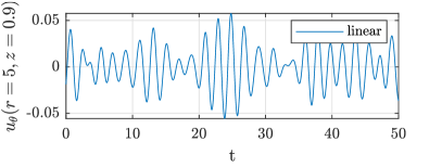
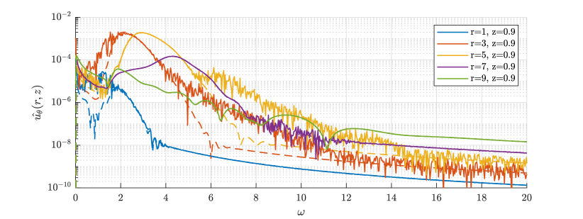
Figure 12: Comparison of linear and nonlinear time integration for $Re=600$, numerical resolution R1. Top: perturbation azimuthal velocity $u_{\theta}$ at location (r=5, z=0.9) from linear (left) and nonlinear time integration (right). Bottom: Corresponding spectrum of non-linear (solid lines) and linear (dashed lines) at $z=0.9$ for various $r$.

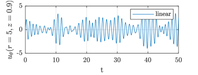
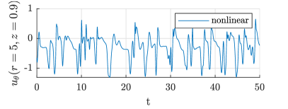
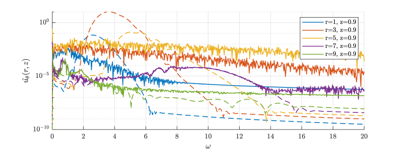
Figure 13: Comparison of linear and nonlinear time integration for $Re=2100$, numerical resolution R1. Top: perturbation azimuthal velocity $u_{\theta}$ at location (r=5, z=0.9) from linear (left) and nonlinear time integration (right). Bottom: Corresponding spectrum of non-linear (solid lines) and linear (dashed lines) at $z=0.9$ for various $r$.

Our goal is now to map in a $(A,Re)$ diagram the different behaviours encountered in the simulations, whether linear or nonlinear. The followed strategy is illustrated in figure 14 by focusing on $Re=2100$. The time series corresponding to the observable $||\omega_{pert}||$ defined by

$$||\omega_{pert}||=\sqrt{\iint|\omega-\omega_{b}|^{2}rdrdz},$$ (24)

where $\omega$ is the azimuthal vorticity and $\omega_{b}$ that of the base flow, are shown in figure 14 (left) in logarithmic scale, and in figure 14 (right) in linear scale, for an amplitude $A$ spanning 6 decades from $A=10^{-12}$ to $A=10^{-6}$ (left) and 6 decades from $A=10^{-7}$ to $A=10^{-1}$ (right). For $A$ from $A=10^{-12}$ to $A=10^{-8}$, the time series in figure 14 (left) differ only by their amplitude which turns out to be proportional to the value of $A$ . For larger $A=10^{-7}$ and especially $10^{-6}$, the time series change aspect and their amplitude no longer follows $A$ linearly. Note that the logarithmic scale is essential for this assessment, by comparison in figure 14(right) is much less easy to interpret along these lines.

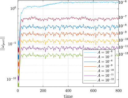
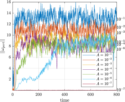
Figure 14: Global observable $||\omega_{pert}||$ in nonlinear time integration at $Re=2100$ for varying forcing amplitude $A$. The values of $A$ are indicated both in the legend and in the plot for simplicity. Starting from $A=10^{-7}$ nonlinear effects are observed. For $A\geq 10^{-6}$ the observable jumps to a different level corresponding to the presence of a non-trivial top branch solution.

This analysis can be repeated for different values of $Re$. In figure 15 (left), the time-averaged $||\omega_{pert}||$ is plotted directly versus the forcing amplitude $A$. This representation allows for a direct assessment of the parameter values for which $||\omega_{pert}||$ scales linearly with $A$, which suggests linear receptivity. All the points lying away from the related straight lines are labelled as nonlinear in the $(A,Re)$ map of figure 15 (right). Beyond the simple linear/nonlinear labelling, we note that for the three largest values of $Re=2100,2400$ and $2700$ in figure 15 (left), the observable $||\omega_{pert}||$ saturates with increasing $A$ to an almost constant level. This suggests that the final state of the simulation is the same whatever $A$, in other words that the forced system is attracted towards a different region of the state space for at least $Re\gtrsim 2100$. A non-trivial chaotic attractor was reported, for the same parameters, for the unforced problem, by Daube & Le Quéré (2002) and Gesla et al. (2023), for $Re\gtrsim 1800$. This attractor is different from the laminar one and it has a different attraction basin in terms of initial condition. There is little doubt that the same attracting chaotic state is identified here in the presence of strong amplitude forcing (the initial condition being fixed). A closer zoom on the figure, especially in linear scale, would show that the saturated value of the observable depends weakly on $A$, which suggests that the associated attractor is gently sensitive to the unsteady forcing. When such an attractor is reached, the corresponding point $(A,Re)$ in the map of figure 15 (right) changes from red to blue. The points that are red correspond to the values of $(A,Re)$ where nonlinear effects do bend the gain curves (left figure), but no finite amplitude state is present and thus no saturation to any non-trivial state can occur. This leads to a 3-colour cartography of the parameter space $(A,Re)$ for the chosen forcing protocol parameterised by the amplitude parameter $A$. The notion of double threshold, popular in the shear flow transition community (Grossmann, 2000), appears here in both $A$ and $Re$ (rather than in initial perturbation amplitude and $Re$), for a forced rather than unforced problem. The boundary between linear and nonlinear behaviour in 15 (right) is consistent with an approximate fit of the form $A=O(Re^{-\alpha})$, with $\alpha\approx 10$. This large value of $\alpha$ is the signature of a very steep boundary. As for the boundary between red (nonlinear) and blue (non-trivial saturation), the present data does not suggest any simple fit. Besides the dataset is known to end at $Re\approx 3000$, beyond which all points are blue because the base flow is linearly unstable and the turbulent state is the only attractor left (Gesla et al., 2023). Rather than a cartography in the $(A,Re)$ plane, where $A$ is specific to a given forcing protocol, we plot in Figure 16 the time-averaged observable $\overline{||\omega_{pert}||}$ versus $Re$, the value of $A$ being treated implicitly. The data is represented using the same colour coding as the preceding figure, both in linear (left figure) and in logarithmic scales (right figure) . In both plots the data corresponding to the non-trivial top and lower branches (i.e. edge states) obtained in Gesla et al. (2023) are also superimposed for clarity (the same observable was used, see their figure 19. The two upper and lower branches from the unforced problem were reported to merge in a saddle-node bifurcation at $Re=Re_{SN}\approx 1800$. Interestingly, none of the red or blue data points, which correspond to the unforced problem, fall in the gap between the lower and upper branch. To our knowledge it is the first time that deterministic data from an unforced problem compares so favourably with data from the forced problem. The right panel of the figure shows the same data in logarithmic scale. There, for the choice of this observable, the boundary between linear and nonlinear behaviour obeys an approximate power-law scaling $\overline{||\omega_{pert}||}=O(Re^{-\beta})$, with $\beta\approx 3.88$.

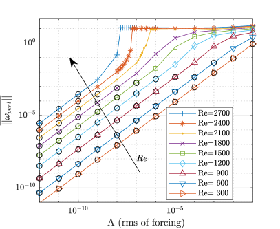
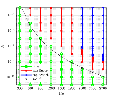
Figure 15: Left: mean observable value $\overline{||\omega_{pert}||}$ as a function of forcing amplitude $A$. The linear regime is indicated using open symbols whenever the slope of the line is at most 1% different from 1. For $Re\geq 2100$ the mean observable value level jumps to the top branch level for strong enough forcing amplitudes. Right: amplitudes corresponding to linear and nonlinear regime indicated respectively with green and red symbols. The top branch is reached for $Re>1800$ whenever $\overline{||\omega_{pert}||}>5$.

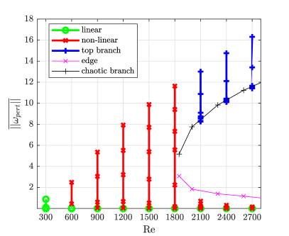
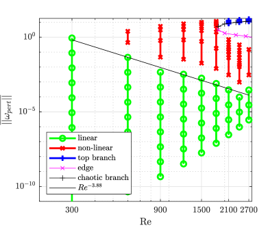
Figure 16: Left: mean observable value $\overline{||\omega_{pert}||}$ as a function of $Re$. The data corresponding to the chaotic solutions from Gesla et al. (2023) are superimposed in respectively blue (top branch) and pink (for the edge branch). Same colour coding as in the previous figure. Right : same data plotted in logarithmic scales.

6.2 Leaky chaotic attractors and finite lifetime dynamics

From the previous subsection, we know that forcing the nonlinear problem with a sufficientlty large amplitude leads, for $Re$ above $Re_{SN}\approx 1800$, to a response different from the response triggered at lower forcing amplitudes. The difference is attested for global observables such as in figure 14 and it is also clear from local velocity probes, as shown in Figure 17 for $Re=2100>Re_{SN}$. In the left panel, low amplitude values $A\leq 10^{-7}$ (corresponding to green points in Figure 15) lead to a disordered response whose diameter increases (linearly) with the value of $A$. In the right panel, only values of $A\geq 10^{-6}$ are displayed and it is apparent again, especially from the numbers along the axes, that the response depends weakly on $A$. This last point suggests the existence of an attracting state independent of $A$, in other words a deterministic attractor, solution of the forced problem, identical to the top-branch solutions identified by Gesla et al. (2023). Similar conclusions can be drawn for all $Re$ larger than 2100, including the supercritical values larger than $Re_{c}\approx 3000$ when only the non-trivial attractor is stable.

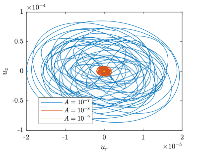
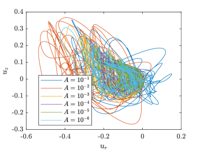
Figure 17: Two-dimensional state portrait $(u_{r},u_{z})$ from a velocity probe located $(r=5,\ z=0.9)$ at $Re=2100$. The width of the state portraits increases linearly with the forcing amplitude for $A\leq 10^{-7}$. For $A\geq 10^{-6}$ state portraits lose their elliptic shape. The center of mass of the state portrait also shifts away from 0, indicating strong nonlinear interaction.

Departures from this picture can however be noted at lower $Re$ close (but above) $Re_{SN}$. Figure 18 shows the outcome several temporal simulations of the unforced problem for $Re=1840$, focusing on the time series of $||\omega_{pert}||(t)$. These time series demonstrate that the chaotic behaviour lasts for a finite time only, after which the observable rapidly reaches zero, indicating a return to the base flow. Some of the measured lifetimes are much longer than the duration of the return to the base flow, which justifies the label supertransient Lai & Tél (2011). The statistics of the lifetimes have been gathered over many such realisations of the deterministic problem, all initialised by different velocity fields drawn randomly. The cumulative distribution of the lifetimes $P(T>t)$, where $T$ is the lifetime, are shown in figure 19(left) for several values of $Re$ between 1800 and 1840. The distributions all look exponential for up to two decades, which suggests a memoryless process (Bottin & Chaté, 1998). The average value $\overline{T}$ of the lifetime is then plotted versus $Re$ in figure 19(right), where the $y$-axis is represented in logarithmic scale. The mean lifetime $\overline{T}$ increases fast with $Re$. Although no functional fit emerges from the data, the growth of $\overline{T}(Re)$ appears faster than exponential. The whole situation is reminiscent from the finite probabilities to relaminarise in three-dimensional turbulence in wall-bounded shear flows, notably the case pipe flow, where lifetimes were reported to increase super-exponentially with $Re$ (Hof et al., 2008). For the case of pipe flow, the academical issue of whether lifetime truly diverge at a finite value of $Re$ or stay finite was solving by remarking that another competing phenomenon, namely turbulence proliferation, would outweigh turbulence decay above some threshold in $Re$ (Avila et al., 2011) and keep turbulence alive for all times. There is no such equivalent here in axisymmetric rotor-stator flow, for which a scenario where lifetimes are always finite is a possibility. Nevertheless, we stress that this debate is essentially academical, the values of $T$ found in practice being so large that they usually exceed the observation times allowed for. In other words, the hypothesis that the invariant set underlying the existence of non-trivial dynamics in the forced problem is a deterministic attractor is only here for commodity : mathematically speaking it could possibly be a leaky attractor i.e. a chaotic saddle (Lai & Tél, 2011).

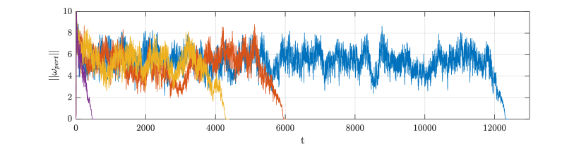
Figure 18: Time series of $||\omega_{pert}||(t)$ for $Re=1840$, unforced problem. Random initial perturbations of amplitude $8\times 10^{-3}$ added to the $u_{\theta}$ component. Four different initial conditions lead to four different lifetime values.

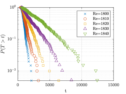
Figure 19: Left: Cumulative distribution function $P(T>t)$ for the lifetime $T$ . $P$ is estimated as the fraction of runs that did not relaminarise in the time interval $(0:t)$. Relaminarisation is decided whenever $||\omega_{pert}||<10^{-3}$. For each value of $Re$ around 200 simulations with different random initial perturbation were conducted. Right: Dependence of the mean lifetime $\overline{T}$ on $Re$. The different data illustrate the sensitivity of the mean lifetime w.r.t. the total number of runs. For a memoryless process the distributions in the left plot would be exactly exponential and the mean lifetime would be the reciprocal of their slope.

7 Conclusions and outlooks

The present numerical investigation has focused on closed axisymmetric rotor-stator flow as a prototype flow for the study of receptivity. Motivated by the riddle about the origin of the dynamical circular rolls observed in several experiments (Savas, 1987; Gauthier, 1998; Schouveiler et al., 2001), both linear and nonlinear receptivity theories were invoked to investigate how the flow responds to an additive forcing of external origin. Several types of forcing were considered, each with its pros and cons. Forcing applied to the bulk of the fluid lends itself well to linear optimal response theory (Schmid & Brandt, 2014). If a wide frequency spectrum is forced, pseudo-resonance linked with non-normal effects (Trefethen & Embree, 2005) will amplify more the frequencies contained in the large hump in the gain curve in fig. 9. Such frequencies invariably lead to circular rolls inside the Bödewadt layer developing along the stator. Forcing applied through motion of the boundaries is by design not optimal, however it is more realistic in the case of closed flows, and can easily be extended to a nonlinear framework. Increasing the amplitude of the forcing at high enough $Re$ unambiguously leads to a different, more complex nonlinear state which coexists with the simpler forced base flow. Although both states are characterised by circular rolls on the stator, we argue that the rolls reported in the experiments of Schouveiler et al. (2001) are a linear response to external forcing and not a self-sustained state like those found by Gesla et al. (2023). This is consistent with the observation that these rolls disappear rapidly should the forcing be suddenly turned off (Lopez et al., 2009; Do et al., 2010). Moreover a particularly striking match with the experiment of Schouveiler et al. (2001) was found when the forcing features only harmonics of the rotor’s main angular frequency, with complex features such as the pairing and merging of vortices well reproduced numerically. The circular rolls observed experimentally can hence be described as noise-sustained, with the subtlety that they are not the response to incoherent noise but rather to a forcing with well-organised frequency content typical of rotating machinery.

As far as the larger picture is concerned, although linear receptivity is the starting point for transition theory based on an input-output picture, any theory aiming at predicting the onset of bistable dynamics needs to be nonlinear. Extending the resolvent formalism to incorporate nonlinear interactions is a possibility (Rigas et al., 2021). As is the case in the present study, the optimality idea from classical linear resolvent theory gets lost in the nonlinear framework in favour of other nonlinear selection criteria. A generalisation of the concept of state space, laminar-turbulent boundary, edge states and other finite-amplitude states to forced problems is awaited for, and seems possible given the encouraging results in figure 16. A clearer connection between the input-output formalism (Sipp & Marquet, 2013), former theories with nonlinear selection criteria in spatially developing flows of global modes (Pier & Huerre, 2001) and the dynamical systems framework would be welcome.

References

- Avila et al. (2011) Avila, K., Moxey, D., De Lozar, A., Avila, M., Barkley, D. & Hof, B. 2011 The onset of turbulence in pipe flow. Science 333 (6039), 192–196.
- Avila & Barkley (2023) Avila, M. & Barkley, D .and Hof, B. 2023 Transition to turbulence in pipe flow. Ann. Rev. Fluid Mech. 55, 575–602.
- Batchelor (1951) Batchelor, G. K. 1951 Note on a class of solutions of the Navier-Stokes equations representing steady rotationally-symmetric flow. Q. J. Mech. Appl. Math. 4, 29–41.
- Bertolotti et al. (1992) Bertolotti, F. P., Herbert, T. & Spalart, P. R. 1992 Linear and nonlinear stability of the blasius boundary layer. J. Fluid Mech. 242, 441–474.
- Bottin & Chaté (1998) Bottin, S. & Chaté, H. 1998 Statistical analysis of the transition to turbulence in plane couette flow. Eur. Phys. J. B 6, 143–155.
- Brady & Durlofsky (1987) Brady, J. F. & Durlofsky, L. 1987 On rotating disk flow. J. Fluid Mech. 175, 363–394.
- Brynjell-Rahkola et al. (2017) Brynjell-Rahkola, M., Shahriari, N., Schlatter, P., Hanifi, A. & Henningson, D. S. 2017 Stability and sensitivity of a cross-flow-dominated falkner–skan–cooke boundary layer with discrete surface roughness. J. Fluid Mech. 826, 830–850.
- Cerqueira & Sipp (2014) Cerqueira, S. & Sipp, D. 2014 Eigenvalue sensitivity, singular values and discrete frequency selection mechanism in noise amplifiers: the case of flow induced by radial wall injection. J. Fluid Mech. 757, 770–799.
- Daube & Le Quéré (2002) Daube, O. & Le Quéré, P. 2002 Numerical investigation of the first bifurcation for the flow in a rotor-stator cavity of radial aspect ratio 10. Comput. Fluids 31, 481–494.
- Do et al. (2010) Do, Y., Lopez, J. M. & Marques, F. 2010 Optimal harmonic response in a confined Bödewadt boundary layer flow. Phys. Rev. E 82 (3), 036301.
- Eckhardt (2018) Eckhardt, B. 2018 Transition to turbulence in shear flows. Phys. A: Stat 504, 121–129.
- Faugaret (2020) Faugaret, A. 2020 Influence of air-water interface condition on rotating flow stability : experimental and numerical exploration. PhD thesis, Sorbonne Université, Paris, France.
- Faugaret et al. (2022) Faugaret, A., Duguet, Y., Fraigneau, Y. & Martin Witkowski, L. 2022 A simple model for arbitrary pollution effects on rotating free-surface flows. J. Fluid Mech. 935, A2.
- Garnaud et al. (2013) Garnaud, X., Lesshafft, L., Schmid, P. J. & Huerre, P. 2013 The preferred mode of incompressible jets: linear frequency response analysis. J. Fluid Mech. 716, 189–202.
- Gauthier (1998) Gauthier, G. 1998 Étude expérimentale des instabilités de l’écoulement entre deux disques. PhD thesis, Université Paris XI, France.
- Gauthier et al. (1999) Gauthier, G., Gondret, P. & Rabaud, M. 1999 Axisymmetric propagating vortices in the flow between a stationary and a rotating disk enclosed by a cylinder. J. Fluid Mech. 386, 105–126.
- Gelfgat (2015) Gelfgat, A. Y. 2015 Primary oscillatory instability in a rotating disk-cylinder system with aspect (height/radius) ratio varying from 0.1 to 1. Fluid Dyn. Res. 47, 035502(14).
- Gesla et al. (2023) Gesla, A., Duguet, Y., Le Quéré, P. & Martin Witkowski, L. 2023 Subcritical axisymmetric solutions in rotor-stator flow. arXiv preprint arXiv:2312.09874 .
- Grossmann (2000) Grossmann, S. 2000 The onset of shear flow turbulence. Rev. Mod. Phys. 72 (2), 603.
- Guermond et al. (2006) Guermond, J. L., Minev, P. D. & Shen, J. 2006 An overview of projection methods for incompressible flows. Comp. Meth. Appl. Mech. Eng. 195, 6011–6045.
- Herbert (1997) Herbert, T. 1997 Parabolized stability equations. Ann. Rev. Fluid Mech. 29 (1), 245–283.
- Hof et al. (2008) Hof, B., De Lozar, A., Kuik, D. J. & Westerweel, J. 2008 Repeller or attractor? selecting the dynamical model for the onset of turbulence in pipe flow. Phys. Rev. Lett. 101 (21), 214501.
- Holodniok et al. (1977) Holodniok, M., Kubicek, M. & Hlavacek, V. 1977 Computation of the flow between two rotating coaxial disks. J. Fluid Mech. 81 (4), 689–699.
- Jin et al. (2021) Jin, B., Symon, S. & Illingworth, S. J. 2021 Energy transfer mechanisms and resolvent analysis in the cylinder wake. Phys. Rev. Fluids 6 (2), 024702.
- Jovanović & Bamieh (2005) Jovanović, M. R. & Bamieh, B. 2005 Componentwise energy amplification in channel flows. J. Fluid Mech. 534, 145–183.
- Lai & Tél (2011) Lai, Y.-C. & Tél, T. 2011 Transient chaos: complex dynamics on finite time scales, , vol. 173. Springer Science & Business Media.
- Launder et al. (2010) Launder, B., Poncet, S. & Serre, E. 2010 Laminar, transitional, and turbulent flows in rotor-stator cavities. Ann. Rev. Fluid Mech. 42, 229–248.
- Lehoucq et al. (1998) Lehoucq, R., Sorensen, D. & Yang, C. 1998 ARPACK users’ guide - solution of large-scale eigenvalue problems with implicitly restarted Arnoldi methods. In SIAM.
- Lopez et al. (2009) Lopez, J. M., Marques, F., Rubio, A. M. & Avila, M. 2009 Crossflow instability of finite Bödewadt flows : Transients and spiral waves. Phys. Fluids 21, 114107.
- Mantič-Lugo et al. (2014) Mantič-Lugo, V., Arratia, C. & Gallaire, F. 2014 Self-consistent mean flow description of the nonlinear saturation of the vortex shedding in the cylinder wake. Phys. Rev. Lett. 113, 084501.
- Pier & Huerre (2001) Pier, B. & Huerre, P. 2001 Nonlinear self-sustained structures and fronts in spatially developing wake flows. J. Fluid Mech. 435, 145–174.
- Poncet et al. (2009) Poncet, S., Serre, E. & Le Gal, P. 2009 Revisiting the two first instabilities of the flow in an annular rotor-stator cavity. Phys. Fluids 21, 064106(8).
- Rigas et al. (2021) Rigas, G., Sipp, D. & Colonius, T. 2021 Nonlinear input/output analysis: application to boundary layer transition. J. Fluid Mech. 911, A15.
- Savas (1987) Savas, O. 1987 Stability of Bödewadt flow. J. Fluid Mech. 183.
- Schmid & Brandt (2014) Schmid, P. J. & Brandt, L. 2014 Analysis of fluid systems: stability, receptivity, sensitivity: lecture notes from the flow-nordita summer school on advanced instability methods for complex flows, stockholm, sweden, 2013. Appl. Mech. Rev. 66 (2), 024803.
- Schouveiler et al. (1998) Schouveiler, L., Le Gal, P. & Chauve, M. P. 1998 Stability of a traveling roll system in a rotating disk flow. Phys. Fluids 10, 2695–2697.
- Schouveiler et al. (2001) Schouveiler, L., Le Gal, P. & Chauve, M. P. 2001 Instabilities of the flow between a rotating and a stationary disk. J. Fluid Mech. 443, 329–350.
- Serre et al. (2001) Serre, E., Crespo Del Arco, E. & Bontoux, P. 2001 Annular and spiral patterns in flows between rotating and stationary discs. J. Fluid Mech. 434, 65–100.
- Serre et al. (2004) Serre, E., Tuliszka-Sznitko, E. & Bontoux, P. 2004 Coupled numerical and theoretical study of the flow transition between a rotating and a stationary disk. Phys. Fluids 16, 688–706.
- Sipp & Marquet (2013) Sipp, D. & Marquet, O. 2013 Characterization of noise amplifiers with global singular modes: the case of the leading-edge flat-plate boundary layer. Theoret. Comput. Fluid Dynamics 27, 617–635.
- Stewartson (1953) Stewartson, K. 1953 On the flow between two rotating coaxial disks. Proc. Camb. Phil. Soc. 49, 333–341.
- Trefethen & Embree (2005) Trefethen, L. N. & Embree, M. 2005 Spectra and pseudospectra: the behavior of nonnormal matrices and operators. Princeton University Press.
- Trefethen et al. (1993) Trefethen, L. N., Trefethen, A. E., Reddy, S. C. & Driscoll, T. A. 1993 Hydrodynamic stability without eigenvalues. Science 261 (5121), 578–584.
- Zandbergen & Dijkstra (1987) Zandbergen, P. J. & Dijkstra, D. 1987 Von kármán swirling flows. Ann. Rev. Fluid Mech. 19 (1), 465–491.