Energy-filtered quantum states and the emergence of non-local correlations

Abstract

Energy-filtered quantum states are promising candidates for efficiently simulating thermal states. We explore a protocol designed to transition a product state into an eigenstate located in the middle of the spectrum; this is achieved by gradually reducing its energy variance, which allows us to comprehensively understand the crossover phenomenon and the subsequent convergence towards thermal behavior. We introduce and discuss three energy-filtering regimes (short, medium and long), and we interpret them as stages of thermalization. We show that the properties of the filtered states are locally indistinguishable from those of time-averaged density matrices, routinely employed in the theory of thermalization. On the other hand, unexpected non-local quantum correlations are generated in the medium regimes and are witnessed by the Rényi entanglement entropies of subsystems, which we compute via replica methods. Specifically, two-point correlation functions break cluster decomposition and the entanglement entropy of large regions scales as the logarithm of the volume during the medium filter time.

Introduction —

In a seminal article, M.C. Bañuls, D. Huse and J.I. Cirac investigated how much entanglement is necessary to reduce the energy fluctuations of a quantum state in the middle of the spectrum of a many-body system [1]. The question is natural: on the one hand, product states have no entanglement but extensive energy fluctuations, on the other hand, the exact eigenstates of Hamiltonians display extensive entanglement entropy. To understand the crossover, they introduced the protocol of energy filtering, which progressively reduces the energy fluctuations of an initial product state. Remarkable was the discovery of intermediate regimes where energy variance shrinks to zero while the entropies grow logarithmically in the system size [1, 2], opening the way to reproducing efficiently thermal properties via pure states [3, 4, 5, 6, 7].

A protocol analogous to filtering is unitary dynamics as, in both cases, purity is preserved but, at late times, the state becomes locally indistinguishable from a thermal one. Quantum correlations spreading across the system during real-time evolution have been thoroughly characterized in order to gain a deeper understanding of the thermalization process. On the other hand, fundamental questions regarding quantum correlations in energy-filtered quantum states (EFQS) are still unanswered. In addition to theoretical interest, clarifying these issues is crucial for understanding the extent to which EFQS can accurately capture thermal properties and to discern features that are instead related to non-thermal spurious effects.

In this Letter, we give a detailed characterization of the behavior of both local observables and entanglement measures during filtering. Remarkably, we find that the EFQS exhibits non-local quantum correlations between arbitrarily distant points. We further develop a technique, based on replica methods, to compute the entanglement entropies of large regions, which complements the information on correlation functions. We find that the intermediate regime of the protocol, characterized by small energy variance and entanglement, is unavoidably accompanied by the violation of the cluster decomposition principle, which is an unorthodox non-thermal feature, albeit thermal features quickly show up locally.

Our approach applies to generic $d$-dimensional systems and provides model-independent predictions; further, it gives a systematic way to characterize the emerging non-local properties and to connect them to the underlying unitary dynamics. We validate our predictions and the actual feasibility of the protocol by testing a non-integrable spin chain with up to $\sim 80$ sites numerically.

Energy filters —

We begin by recalling a few known results on EFQS. We consider a local Hamiltonian $H$ and a product state $\ket{\Psi_{0}}$ that is not an energy eigenstate and such that $E_{\Psi_{0}}=\bra{\Psi_{0}}H\ket{\Psi_{0}}$ lies in the middle of the energy spectrum. We construct the EFQS as follows:

$$\ket{\Psi_{\tau}}=\frac{1}{\sqrt{\mathcal{Z}(\tau)}}\exp\left(-\frac{(H-E_{\Psi_{0}})^{2}}{4}\tau^{2}\right)\ket{\Psi_{0}};$$ (1)

the operator acting on $\ket{\Psi_{0}}$ is the energy filter and $\tau$ the filter time; $\mathcal{Z}(\tau)$ ensures normalisation. The energy variance of $\ket{\Psi_{\tau}}$ decreases as $\tau$ increases, and $\ket{\Psi_{\tau}}$ interpolates between the initial product state $\ket{\Psi_{0}}$ and a state with reduced energy fluctuations maintaining the same energy. Without loss of generality, we can assume $E_{\Psi_{0}}=0$ (the Hamiltonian can be shifted by a constant).

The energy distribution of $\ket{\Psi_{\tau}}$ can be determined under weak assumptions. For a product state $\ket{\Psi_{0}}$, all the cumulants of $H$ are extensive, the central limit theorem holds, and the energy distribution of $\ket{\Psi_{0}}$ is Gaussian in the large volume $V$ limit [8]. This means that for a typical eigenstate $\ket{E}$ with energy $E$ the scalar product $|\langle E|\Psi_{0}\rangle|^{2}\propto\exp\left(-\frac{E^{2}}{2\varepsilon_{2}V}\right),$ where $\varepsilon_{2}V\equiv\Delta H^{2}_{0}$ is the energy variance of $\ket{\Psi_{0}}$. From Eq. (1) we can compute the energy distribution of the filtered state $|\langle E|\Psi_{\tau}\rangle|^{2}\propto\exp\left(-\frac{E^{2}\tau^{2}}{2}\right)|\langle E|\Psi_{0}\rangle|^{2}$, so that the variance of $\ket{\Psi_{\tau}}$ is

$$\Delta H^{2}_{\tau}\simeq\frac{1}{\tau^{2}+\frac{1}{\varepsilon_{2}V}}.$$ (2)

Filtering regimes —

The formula in Eq. (2) suggests the identification of three filtering regimes. We list them here and anticipate some of the results derived below. At short filter time, $\tau\sim\frac{1}{\sqrt{V}}$, the energy variance is extensive and the expectation value of local observables is close to the initial value; entanglement starts to build up, but the state remains a standard area-law state. At medium filter time, $\tau\sim O(1)$, the energy variance does not scale anymore with the size of the system. Bipartite entanglement entropies become significant and have a universal scaling as $\frac{1}{2}\log V_{A}$, where $V_{A}$ is the volume of the smallest region $A$ (reminiscent of the logarithmic behavior found in long-range systems in Refs. [9, 10]). Here, a new phenomenology appears: the state breaks the clustering condition and quantum correlations become highly non-local. Finally, at long filter times, when $\tau$ increases with $V$, local observables attain values that are independent of $\tau$. The bipartite entanglement entropy scales as the volume $\sim V_{A}$ and two-point correlation functions satisfy again a clustering condition; the state can be considered as thermal.

Local observables —

The study of EFQS is not straightforward because $\ket{\Psi_{\tau}}$ in Eq. (1) is issued from a non-local and non-Hermitian evolution. Our approach is based on the existence of a deep link with the process of thermalization that we detail below.

We begin with a representation of $\ket{\Psi_{\tau}}$ obtained by Fourier-transforming the energy filter (see also Refs. [11, 12, 1])

$$\ket{\Psi_{\tau}}\propto\int^{\infty}_{-\infty}dt^{\prime}\lambda_{\tau}(t^{\prime})e^{-iHt^{\prime}}\ket{\Psi_{0}},\;\;\lambda_{\tau}(t)=\exp\bigl(-\tfrac{t^{2}}{\tau^{2}}\bigr{missing}).$$ (3)

Eq. (3) provides a link between the filtered state and the time-evolving one $\ket{\Psi_{0}(t)}=e^{-iHt}\ket{\Psi_{0}}$. We now consider a local observable $\mathcal{O}$  in the Heisenberg picture, $\mathcal{O}(t)=e^{iHt}\mathcal{O}e^{-iHt}$. Formally, its expectation value in $\ket{\Psi_{\tau}}$, which we denote by $\langle\ldots\rangle_{\tau}$, reads

$$\langle\mathcal{O}(t)\rangle_{\tau}=\frac{\int d\tilde{t}_{1}dt_{1}\lambda_{\tau}^{*}(\tilde{t}_{1})\lambda_{\tau}(t_{1})\langle e^{iH(\tilde{t}_{1}-t_{1})}\mathcal{O}(t-t_{1})\rangle_{0}}{\int d\tilde{t}_{1}dt_{1}\lambda_{\tau}^{*}(\tilde{t}_{1})\lambda_{\tau}(t_{1})\langle e^{iH(\tilde{t}_{1}-t_{1})}\rangle_{0}}.$$ (4)

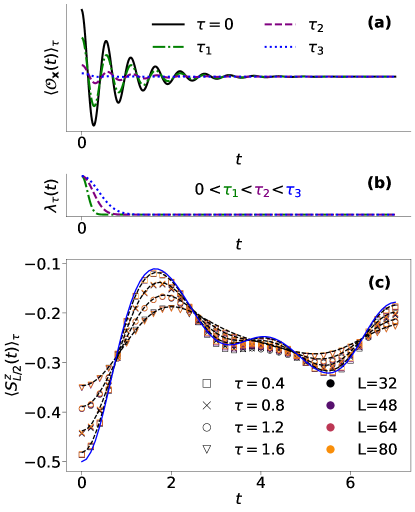
Figure 1: A sketch of $\langle\mathcal{O}_{\mathbf{x}}(t)\rangle_{\tau}$ as a function of $t$ for different values of $\tau$ is shown in panel (a). The data are produced using Eq. (5) and we plot the profile of the filter kernel $\lambda_{\tau}(t)$ that we employed in panel (b). In panel (c) we show actual numerical results for the model discussed at the end of the letter in Eq. (12). The markers represent the numerical data obtained for the numerically-simulated filtered state, while the blue line shows the expectation value of the observable for the unfiltered state $\ket{\Psi_{0}(t)}$. The comparison with the black dotted lines, which are evaluated via the right-hand side of Eq. (5), is excellent at several system sizes $L$.

We point out that, in the limit of large system $V\rightarrow\infty$ with $t,\tau$ fixed, this can be simplified: On the one hand, at the denominator the expectation value $\langle e^{iH(\tilde{t}_{1}-t_{1})}\rangle_{0}$ is the Loschmidt echo, or return amplitude, which scales as $e^{VF(t_{1}-\tilde{t}_{1})}$ , with $F(t)$ a function that is analytic in a neighborhood of $t=0$, when $\ket{\Psi_{0}}$ is a product state [15, 16]. On the other hand, such an exponential localisation in time characterises also the numerator $\langle e^{iH(\tilde{t}_{1}-t_{1})}\mathcal{O}(t-t_{1})\rangle_{0}$, which turns out to scale as $e^{VF(t_{1}-\tilde{t}_{1})}\langle\mathcal{O}(t-t_{1})\rangle_{0}$. We can then perform the integrals over $\tilde{t}_{1}$ in Eq. (4), which are marked by a saddle point contribution localized at $\tilde{t}_{1}\simeq t_{1}$. This gives the first main result:

$$\langle\mathcal{O}(t)\rangle_{\tau}\simeq\frac{\int dt_{1}|\lambda_{\tau}(t_{1})|^{2}\langle\mathcal{O}(t+t_{1})\rangle_{0}}{\int dt_{1}|\lambda_{\tau}(t_{1})|^{2}}.$$ (5)

Hence, the EFQS $\ket{\Psi_{\tau}}$ is locally indistinguishable from the time-averaged mixed state that is routinely invoked in the theory of thermalisation [17, 4]

$$\rho_{th}(\tau)\propto\int dt_{1}\,|\lambda_{\tau}(t_{1})|^{2}\,\ket{\Psi_{0}(t_{1})}\bra{\Psi_{0}(t_{1})}.$$ (6)

Eqs. (5) and (6) are a powerful tool for linking the physics of EFQS to the theory of thermalization, as we discuss below—see also Fig. 1. Let us consider for simplicity $t=0$ in Eq. (5) and a local observable $\mathcal{O}$. For small $\tau$, $\langle\mathcal{O}(0)\rangle_{\tau}$ is dominated by the initial transient dynamics of $\langle\mathcal{O}(t_{1})\rangle_{0}$. For large $\tau$, it is dominated by times $t_{1}$ larger than the observable’s relaxation time, and, thus, $\langle\mathcal{O}(0)\rangle_{\tau}$ converges to its thermal value. The medium filter time captures how thermalization occurs dynamically and is therefore a particularly intriguing regime.

The goal of the rest of the paper is to show that energy filtering is a powerful method for understanding this process, so far largely unexplored, and we will do so by deriving some general and universal properties that characterize the medium filter time.

Two-point correlations —

Let us focus on short or medium filter times and consider two operators $\mathcal{O}_{\mathbf{x}}$ and $\mathcal{O}_{\mathbf{y}}$, localized at $\mathbf{x},\mathbf{y}$, at a distance large enough to cluster in the state $e^{-iH\tau}\ket{\Psi_{0}}$. Eq. (5) can then be simplified as follows

$$\langle\mathcal{O}_{\mathbf{x}}\mathcal{O}_{\mathbf{y}}\rangle_{\tau,c}\simeq\frac{\int dt_{1}|\lambda_{\tau}(t_{1})|^{2}\langle\mathcal{O}_{\mathbf{x}}(t_{1})\rangle^{2}_{0}}{\int dt_{1}|\lambda_{\tau}(t_{1})|^{2}}-\langle\mathcal{O}_{\bf x}\rangle_{\tau}^{2},$$ (7)

where translational invariance has been employed. This correlator satisfies the clustering condition if, for large enough $|\mathbf{x}-\mathbf{y}|$, it is equal to zero.

At short filter times, where $|\lambda_{\tau}(t)|^{2}$ localizes at $t\simeq\leavevmode\nobreak\ 0$, $\langle\mathcal{O}_{\mathbf{x}}\mathcal{O}_{\mathbf{y}}\rangle_{\tau,c}$ vanishes because the initial state $\ket{\Psi_{0}}$ is a product state. For medium $\tau$, instead, the right-hand side of Eq. (7) is nonzero simply because the operator is time evolving—we will provide numerical evidence in Fig. 2. In that regime, therefore, the state $\ket{\Psi_{\tau}}$ breaks the clustering condition and its correlations become non-local. This is consistent with the fact that the energy filter introduced in Eq. (1) comes from a non-local time evolution. We can conclude that, during the energy filtering, non-local and non-thermal correlations build up, and, in turn, $\rho_{th}$ shall develop similar properties before approaching a thermal state.

Entanglement of bipartitions —

We now investigate quantum correlations between spatial regions through the lens of entanglement. We recall that, given a quantum state and denoting by $\rho_{A}$ its reduced density matrix with respect to a region $A$ with volume $V_{A}$, its $n$-th Rényi entropy reads $S_{n}(A)\equiv(1-n)^{-1}\log\text{Tr}\left(\rho^{n}_{A}\right)$ and the von Neumann entropy is $S_{1}(A)\equiv-\text{Tr}\left(\rho_{A}\log\rho_{A}\right)$. We compute the Rényi entropies $S_{n,\tau}(A)$ ($n\geq 2$) for the filtered state $\ket{\Psi_{\tau}}$ with the replica method, which requires to compute $\text{Tr}\left(\rho^{n}_{A}\right)$ as a certain partition function between $n$ replicas; we then use the replica trick to compute the von Neumann entropy, i.e., we perform the analytical continuation over $n\in\mathbb{R}_{>0}$ and take the limit $n\rightarrow 1^{+}$ [18]. After introducing the twist operator $\mathcal{T}_{A}$, that acts as a replica permutation $j\rightarrow j+1$ (with $j=1,\dots,n$ a replica index) within the region $A$, we can represent the moments of $\rho_{A}$ as $\text{Tr}\left(\rho^{n}_{A}\right)=\,^{n}\bra{\Psi}\mathcal{T}_{A}\ket{\Psi}^{n}$, with $\ket{\Psi}^{n}\equiv\ket{\Psi}^{\otimes n}$ the state of the system replicated $n$ times [19, 20, 21]. Details on the actual calculations are reported in the Supplementary Material (SM); here we focus on the results.

At short filter times $\tau\sim 1/\sqrt{V}$, entanglement starts to build up quickly, and we find

$$S_{n,\tau}(A)-S_{n,0}(A)=f_{\mathrm{sft},n}\left(\sqrt{\varepsilon_{2}V}\tau,\frac{V_{A}}{V}\right).$$ (8)

In the case of a product state $S_{n,0}(A)$ is zero, but the result holds more generally for an initial area-law state. The explicit form of $f_{\mathrm{sft},n}$ is universal and it does not depend on the details of the Hamiltonian; it is reported in the SM. In particular, it first grows quadratically as $f_{\mathrm{sft},n}\sim V\tau^{2}$, whereas asymptotically the behaviour is logarithmic, $f_{\mathrm{sft},n}\sim\log(\sqrt{V}\tau)$.

After this transient, at a filter time scaling as $\tau\sim 1/\sqrt{V}$, the entropy reaches a value proportional to the logarithm of $V_{A}$. This result is non-trivial as a priori one would expect that a non-local evolution saturates the quantum correlations and produces an entanglement of bipartition scaling as $V_{A}$.

The medium filter time regime takes place after this saturation and we obtain

$$S_{n}(A)-S_{n,0}(A)\simeq\frac{1}{2}\log V_{A}+g_{\mathrm{mft},n}(\tau)+\ldots.$$ (9)

The function $g_{\mathrm{mft},n}(\tau)$, represents the most important contribution that appears as a function of $\tau$. In particular, the behaviour above is found for $\tau$ shorter than the time that is necessary for the subsystem to thermalize.

The explicit expression of $g_{\mathrm{mft},n}(\tau)$ depends on the model, but its asymptotic behavior in $\tau$ has general features; we find a strong dependence on the order of the Rényi entropy, a situation which is rather uncommon:

$$g_{\mathrm{mft},n}(\tau)\simeq\begin{cases}\frac{n}{n-1}\log\tau,&n>1;\\ \frac{1}{\sqrt{2\pi}}\Gamma_{1}\,|\partial A|\tau,&n=1;\\ \frac{1-n}{8n}\Gamma^{2}_{n}\,|\partial A|^{2}\tau^{2},&0<n<1.\\ \end{cases}$$ (10)

Here, the growth of entropy under unitary dynamics is assumed to be linear, and $\Gamma_{n}$ is related to its rate via $S_{n}(A)\simeq\Gamma_{n}\,|\partial A|t$. The linear growth of $S_{1}(A)$ as a function of $\tau$ in Eq. (10) has to be compared with the slower logarithmic growth observed for $n>1$, and it is compatible with the rigorous upper bound found in Ref. [1] with different methods for one-dimensional systems. We mention that a similar drastic change of behaviour of the Rényi entropy close to $n=1$ has been found also in a different context in Refs. [22, 23]. Interestingly, this change of behavior disappears when $A$ is taken to be the entire system [17].

The Rényi entropies for $0<n<1$ are fundamental in the context of tensor networks; in particular, it is known that if $S_{n}(A)$ is bounded by $c\log V_{A}$, then an efficient MPS representation exists [24]. Our result in Eq. (10), therefore, suggests that the filtered state $\ket{\Psi_{\tau}}$ can be efficiently simulated with a tensor-network algorithm up to a filter time of order $\tau\sim\sqrt{\log V}.$ This would make it accessible to a classical simulation a state with logarithmic entanglement entropy and an energy variance decaying as $\Delta H^{2}_{\tau}\sim\frac{1}{\log V}$. A rigorous proof of a similar statement has been provided in Ref. [2] with different methods for one-dimensional systems.

We remind the reader that Ref. [25] found asymptotic eigenstates with subextensive entanglement entropy and energy variance $\Delta H^{2}\sim\frac{1}{L^{2}}$. We note that such a scenario cannot be recovered via the filter protocol for generic systems because $\tau\sim V$ is a time scale compatible with the thermalization time, when every region has thermalized and an extensive entropy is observed.

Mutual information —

We remark that the prefactor ($1/2$) of the logarithmic growth of the entropy as a function of the volume in Eq. (9) holds for both connected and disconnected regions. In particular, the mutual information of two distant regions $A,B$ of size $V_{A},V_{B}=V_{A}$ can be estimated as

$$I(A,B)\equiv S_{1}(A)+S_{1}(B)-S_{1}(A\cup B)\simeq\frac{1}{2}\log V_{A}+\dots$$ (11)

up to $O(1)$ terms (finite for $\tau\neq 0$ fixed and $V_{A}$ large). Therefore, the mutual information does not decay to zero within the distance, as it happens in the ground states of critical systems [26]. Similar properties are also found in some exact scars (see Ref. [27]), and they are ultimately related to the breaking of clustering. This is the entanglement version of the non-locality of the state at medium filter time that has been pointed out when looking at two-point correlation functions.

Numerical simulations —

We benchmark our predictions against numerical results in a one-dimensional quantum spin chain of length $L$. We consider the spin-1/2 Ising model with both longitudinal and transverse magnetic field

$$H=-J\sum_{j=1}^{L-1}{S^{x}_{j}S^{x}_{j+1}}+h_{x}\sum_{j=1}^{L}{S^{x}_{j}}+h_{z}\sum_{j=1}^{L}{S^{z}_{j}};$$ (12)

with open boundary conditions, and we choose $J=1,h_{x}=1.2,h_{z}=0.8$. We take $\ket{\Psi_{0}}=\ket{\uparrow\downarrow\uparrow\downarrow\ldots\uparrow\downarrow}$, which lies in the middle of the spectrum with $E_{\Psi_{0}}=0$ and has extensive energy variance $\Delta H^{2}_{0}=(J^{2}/16+h_{x}^{2}/4)L$. In order to numerically implement the energy filter $e^{-\frac{H^{2}\tau^{2}}{4}}$ we use a matrix-product state representation of the quantum state combined with the Time-Dependent Variational Principle (TDVP) [28, 29, 30], employing the ITensors library [31, 32]. We follow Ref. [33] and we first apply the 2-TDVP until a chosen bond-link $\chi=450$ is reached; subsequently, we employ the 1-TDVP algorithm at fixed bond link. This procedure represents a compromise between the computational efficiency offered by 1-TDVP, and the mitigation of projection errors inherent to 2-TDVP. This allows us to reliably simulate chains of up to $L=80$ sites up to filter time $\tau=7$.

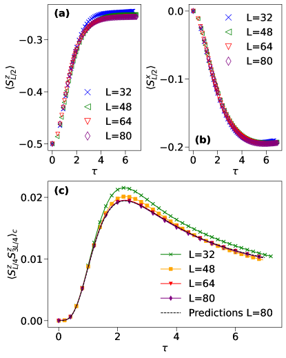
Figure 2: Panels (a) and (b) show the evolution of $\langle S^{z}_{j=\frac{L}{2}}\rangle_{\tau}$ and $\langle S^{x}_{j=\frac{L}{2}}\rangle_{\tau}$, as function of $\tau$. In (c) we show results for the connected correlator $\langle S^{z}_{j=\frac{L}{4}}S^{z}_{j^{\prime}=\frac{3L}{4}}\rangle_{\tau,c}$, as function of $\tau$. We compare numerical data for $L=32,48,64,80$ with the right-hand side of Eq. (7) evaluated for $L=80$.

We first assess the validity of Eq. (5). In Fig. 1(c) we plot the numerical data obtained for $\langle\mathcal{O}(t)\rangle_{\tau}$, with $\mathcal{O}=S^{z}_{j=\frac{L}{2}}$. Black dashed curves are obtained by processing, according to Eq. (5), the unitary time-evolution result $\langle\mathcal{O}(t)\rangle_{0}$, which is plotted as a solid blue line. The comparison with the direct simulation of $\langle\mathcal{O}(t)\rangle_{\tau}$ using the filter algorithm is excellent.

We subsequently investigate the behaviour of local observables and of two-point connected correlation functions of distant points, studying $\langle S^{z}_{j=\frac{L}{2}}\rangle$, $\langle S^{x}_{j=\frac{L}{2}}\rangle$ and $\langle S^{z}_{j=\frac{L}{4}}S^{z}_{j^{\prime}=\frac{3L}{4}}\rangle_{\tau,c}$ and plot the results in Fig. 2. Local observables have a significant dependence on the filter time up to $\tau\sim 4$, after which they show significant saturation effects; it is expected that this value is close to the thermal one approached for $\tau\to\infty$. As anticipated, the connected correlator takes the value $0$ at $\tau=0$, increases towards a maximal value, and eventually decreases for longer values of $\tau$. The curves obtained at various $L$ are compatible with a collapse as $L$ increases. We also evaluate numerically for $L=80$ the right-hand side of Eq. (7), obtained from the unitary dynamics of the model, finding good agreements with the previous curves. Note that while local observables have saturated and approach slowly the long-$\tau$ limit, the connected correlation function is still displaying a significant evolution, with a marked decreasing trend.

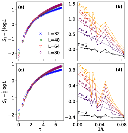
Figure 3: $S_{n}-1/2\log L$ ($n=1,2$) for the half-chain bipartition as a function of $\tau,L$. The data against $\tau$ (panels (a) and (c)) show compatibility with a collapse as $L$ increases. In (b) and (d) we show the results as a function of $1/L$ for different values of $\tau$ and extrapolate them in the limit $L\to\infty$. The extrapolated value is finite, which supports the anticipated large-$L$ behaviour $S_{1,2}\sim\frac{1}{2}\log L$.

Finally, we study the Rényi entropies ($n=1,2$) of half-chain in the medium filter time as a function of $\tau$ and system size $L$; the results are plotted in Fig. 3. Our data show compatibility with a collapse of $S_{n}-\frac{1}{2}\log L$ against $\tau$, as predicted by Eq. (9). Finite-size deviations are displayed in panels (b) and (d), and a slowly-decaying oscillating behaviour as a function of $L$ is found.

Conclusions —

We have shown that the filtering protocol generates non-local correlations in an intermediate filter-time regime. These non-thermal effects should be contrasted with the local thermal features, which emerge quickly. We provide analytical predictions for entanglement entropies and its fictitious dynamics under filtering that address fundamental questions regarding the simulability of thermal properties via quantum pure states, and that have been thoroughly validated through numerical simulation.

Further, we believe that the techniques employed, concerning a non-local and non-unitary evolution, can be applied in the context of open quantum systems. Another interesting direction regards the possible role of conserved charges, or integrability, in the filtering. Non-thermal states, say generalized Gibbs ensembles, are then expected to arise eventually after filtering. We defer the examination of these generalizations to future investigations.

Supplementary Material for
“Energy-filtered quantum states and the emergence of non-local correlations”

Appendix A Rényi entropies and replica trick

In this section, we characterize the Rényi entropy of the filtered state $\ket{\Psi_{\tau}}$ via replica trick. Given a subsystem $A$, we first express the $n$th moment of its RDM as

$$\begin{split}&\text{Tr}\left(\rho^{n}_{A}\right)=^{n}\bra{\Psi_{\tau}}\mathcal{T}_{A}\ket{\Psi_{\tau}}^{n}=\frac{1}{\left(\int d\tilde{t}_{1}dt_{1}\lambda(\tilde{t}_{1})\lambda_{\tau}(t_{1})\langle e^{iH(\tilde{t}_{1}-t_{1})}\rangle_{0}\right)^{n}}\times\\ &\int d\tilde{t}_{1}dt_{1}\dots d\tilde{t}_{n}dt_{n}\lambda_{\tau}(\tilde{t}_{1})\dots\lambda_{\tau}(\tilde{t}_{n})\lambda_{\tau}(t_{1})\dots\lambda_{\tau}(t_{n})\times^{n}\bra{\Psi_{0}}e^{i\sum_{j}H_{j}\tilde{t}_{j}}\mathcal{T}_{A}e^{-i\sum_{j}H_{j}t_{j}}\ket{\Psi_{0}}^{n},\end{split}$$ (13)

with $H_{j}$ the Hamiltonian of the $j$-th replica. The expression above, exact at finite size, boils down to a computation of an integral in $2n$ variables. Simplifications occur in the limit of large regions, and one can exploit the exponential localization of the integrand (analogous to the Loschmidt echo case, discussed in the main text). For instance, ${}^{n}\bra{\Psi_{0}}e^{i\sum_{j}H_{j}\tilde{t}_{j}}\mathcal{T}_{A}e^{-i\sum_{j}H_{j}t_{j}}\ket{\Psi_{0}}^{n}$ gets a contribution from the region $A$ associated with the replica shift: this gives localization around $t_{j-1}\simeq\tilde{t}_{j}$. Another contribution comes from the complementary region, and it gives localization around $t_{j}\simeq\tilde{t}_{j}$. We perform a quadratic approximation around the localization points, relevant to evaluate the integral in Eq. (LABEL:eq:Exp_twist), and we get

$$\begin{split}&{}^{n}\bra{\Psi_{0}}e^{i\sum_{j}H_{j}\tilde{t}_{j}}\mathcal{T}_{A}e^{-i\sum_{j}H_{j}t_{j}}\ket{\Psi_{0}}^{n}\simeq\exp\left(-\frac{\varepsilon_{2}(V-V_{A})}{2}\sum_{j}(t_{j}-\tilde{t}_{j})^{2}-\frac{V_{A}\varepsilon_{2}}{2}\sum_{j}(t_{j-1}-\tilde{t}_{j})^{2}\right)\times{}^{n}\bra{\Psi_{0}}\mathcal{T}_{A}(t_{1})\ket{\Psi_{0}}^{n}.\end{split}$$ (14)

Here, ${}^{n}\bra{\Psi_{0}}\mathcal{T}_{A}(t_{1})\ket{\Psi_{0}}^{n}$ is the $n$th moment of the RDM in the state $\ket{\Psi_{0}(t_{1})}$, and it is the only quantity which contains detail on the underlying model.

We first discuss the short filter time $\tau\sim\frac{1}{\sqrt{V}}$ and for convenience we define the rescaled variable

$$\tilde{\tau}=\sqrt{V}\tau.$$ (15)

The integral in Eq. (LABEL:eq:Exp_twist) is a Gaussian integral over $2n$ variables. Because of the fast decay of $\lambda_{\tau}(t)$ as a function of $t$, the integrand is localized around $t_{j}\simeq\tilde{t}_{j}\simeq 0$; in this regime we can therefore safely replace ${}^{n}\bra{\Psi_{0}}\mathcal{T}_{A}(t_{1})\ket{\Psi_{0}}^{n}$ by ${}^{n}\bra{\Psi_{0}}\mathcal{T}_{A}(0)\ket{\Psi_{0}}^{n}$ inside (LABEL:eq:Exp_twist). The latter is $1$ for a product state, but the forthcoming discussion will hold true for area-law states as well. We introduce the $2n$-dimensional vector

$$\mathbf{t}=\begin{pmatrix}t_{1}\\ \dots\\ t_{n}\\ \tilde{t}_{1}\\ \dots\\ \tilde{t}_{n}\end{pmatrix},$$ (16)

and we express the numerator of (LABEL:eq:Exp_twist) as

$${}^{n}\bra{\Psi_{0}}\mathcal{T}_{A}(0)\ket{\Psi_{0}}^{n}\times\int d\mathbf{t}\exp\left(-\frac{1}{2}V\mathbf{t}^{T}\mathbf{M}_{n}\mathbf{t}\right)={}^{n}\bra{\Psi_{0}}\mathcal{T}_{A}(0)\ket{\Psi_{0}}^{n}\times{\det}^{-\frac{1}{2}}\left(\frac{V\mathbf{M}_{n}}{2\pi}\right),$$ (17)

with $\mathbf{M}_{n}$ the $2n\times 2n$ matrix $\mathbf{M}_{n}$

$$\begin{split}\mathbf{M}_{n}=\left(\frac{2}{\tilde{\tau}^{2}}+\varepsilon_{2}\right)\mathds{1}+\varepsilon_{2}(1-V_{A}/V)\begin{pmatrix}0&\vline&-\mathds{1}\\ \hline\cr-\mathds{1}&\vline&0\end{pmatrix}+\varepsilon_{2}V_{A}/V\begin{pmatrix}\begin{matrix}0&\dots&\dots&0\\ \dots&\dots&\dots&\dots\\ \dots&\dots&\dots&\dots\\ 0&\dots&\dots&0\end{matrix}&\vline&\begin{matrix}0&-1&0&\dots\\ \dots&0&-1&\dots\\ \dots&\dots&\dots&\dots\\ -1&0&0&\dots\end{matrix}\\ \hline\cr\begin{matrix}0&\dots&\dots&-1\\ -1&0&\dots&0\\ 0&-1&\dots&0\\ \dots&\dots&\dots&\dots\end{matrix}&\vline&\begin{matrix}0&\dots&\dots&0\\ \dots&\dots&\dots&\dots\\ \dots&\dots&\dots&\dots\\ 0&\dots&\dots&0\end{matrix}\end{pmatrix},\end{split}$$ (18)

whose spectrum is thoroughly discussed in Sec. B. Finally, we compute the difference of Rényi entropies between $\ket{\Psi_{\tau}}$ and $\ket{\Psi_{0}}$ as

$$S_{n}(A)=S_{n,0}(A)+\frac{1}{2(n-1)}\log\frac{\det(\mathbf{M}_{n})}{\det^{n}(\mathbf{M}_{1})}.$$ (19)

For small $\tilde{\tau}$ one gets a quadratic growth as $S_{n}(A)-S_{n,0}(A)\sim\tilde{\tau}^{2}$. For large $\tilde{\tau}$ instead a logarithmic growth is observed

$$S_{n}(A)-S_{n,0}(A)\simeq\log\tilde{\tau}+\dots,$$ (20)

which will be traced back to the smallest eigenvalue of $\mathbf{M}_{n}$. As expected, our prediction vanishes identically in the limit $V_{A}/V\rightarrow 0$; this is a further demonstration that local observables, associated with a finite region $A$, do not vary in the short filter time regime (see Eq. (19)). Further, one can check explicitly that the result is symmetric under $V_{A}\leftrightarrow V-V_{A}$, as expected since $\ket{\Psi_{\tau}}$ is a pure state.

In the case of a medium filter time, with $\tau$ fixed, one can still perform a saddle-point analysis, but carefulness is needed. In particular, $\lambda_{\tau}(t_{j})$ (and $\lambda_{\tau}(\tilde{t}_{j})$) no longer contribute to the saddle point of (LABEL:eq:Exp_twist), and the latter is determined by the term in Eq. (14). Here localization of the integral around $t_{j}\simeq\tilde{t}_{j}\simeq t$, which is a one-dimensional manifold, occurs. To compute (LABEL:eq:Exp_twist), we first perform a saddle-point integration over the transverse ($2n-1$) directions and, then, integrate over $t$

$$\begin{split}{}^{n}\bra{\Psi_{\tau}}\mathcal{T}_{A}\ket{\Psi_{\tau}}^{n}=\frac{\int dt|\lambda_{\tau}(t)|^{2n}\ {}^{n}\bra{\Psi_{0}}\mathcal{T}_{A}(t)\ket{\Psi_{0}}^{n}}{\left(\int dt|\lambda_{\tau}(t)|^{2}\right)^{n}}\times\frac{\int d\mathbf{t}\exp\left(-\frac{1}{2}V\mathbf{t}^{T}\mathbf{N}_{n}\mathbf{t}\right)}{\left(\int dt^{\prime}\exp\left(-\frac{1}{2}Vt^{\prime}\mathbf{N}_{1}t^{\prime}\right)\right)^{n}}=\\ \frac{\int dt|\lambda_{\tau}(t)|^{2n}\ {}^{n}\bra{\Psi_{0}}\mathcal{T}_{A}(t)\ket{\Psi_{0}}^{n}}{\left(\int dt|\lambda_{\tau}(t)|^{2}\right)^{n}}\times\left(\frac{V}{2\pi}\right)^{\frac{1-n}{2}}\times\frac{\text{det}^{-\frac{1}{2}}\left(\mathbf{N}_{n}\right)}{\text{det}^{-\frac{n}{2}}\left(\mathbf{N}_{1}\right)}\end{split}$$ (21)

where $\mathbf{t}$ is the $2n-1$-dimensional vector

$$\mathbf{t}=\begin{pmatrix}t_{1}\\ \dots\\ t_{2n-1}\end{pmatrix},$$ (22)

and $\mathbf{N}_{n}$ is a $2n-1\times 2n-1$ matrix. The specific entries of $\mathbf{N}_{n}$ depend on the way we parametrize the $2n-1$-dimensional manifold that is orthogonal to the one-dimensional one where the integral localizes. However, the spectrum of $\mathbf{N}_{n}$ does not depend on this choice and it can be obtained directly from the results available for $\mathbf{M}_{n}$ in Sec. B. For instance, in the limit $\tilde{\tau}\rightarrow+\infty$ in Eq. (18), $\mathbf{M}_{n}$ becomes singular as one eigenvalue vanishes: this eigenvalue is associated precisely with the one-dimensional manifold of localization ($t_{j}=\tilde{t}_{j}=t$ in Eq. (LABEL:eq:Exp_twist)), while the other ($2n-1$) ones rule the exponential decay in its neighborhood. The latter are the eigenvalues of $\mathbf{N}_{n}$, and we write the spectrum of the matrix (denoted by $\text{Spec}(\dots)$) as

$$\text{Spec}\left(\mathbf{M}_{n}|_{\tilde{\tau}=\infty}\right)=\text{Spec}\left(\mathbf{N}_{n}\right)\cup\{0\}.$$ (23)

For completeness, we write the eigenvalues of $\mathbf{N}_{n}$ as

$$\begin{split}\{\varepsilon_{2}(1+\sqrt{(1-V_{A}/V)^{2}+(V_{A}/V)^{2}+2V_{A}/V(1-V_{A}/V)\cos k})\}_{k\geq 0}\cup\\ \{\varepsilon_{2}(1-\sqrt{(1-V_{A}/V)^{2}+(V_{A}/V)^{2}+2V_{A}/V(1-V_{A}/V)\cos k})\}_{k>0},\end{split}$$ (24)

with $k\in\frac{2\pi}{n}\{0,\dots,n-1\}$.

To proceed with the analysis, it is necessary to make some hypothesis on the behaviour of ${}^{n}\bra{\Psi_{0}}\mathcal{T}_{A}(t)\ket{\Psi_{0}}^{n}$, which is the only quantity not predicted by this approach and depends on the properties of the model. We assume that the growth in time of the entropy under unitary dynamics from the state $\ket{\Psi_{0}}$ is linear, which is a common scenario found for both integrable and non-integrable systems [36, 37, 38]. At large times, the entropy is expected to approach an extensive value, and hence

$$\begin{split}&\frac{{}^{n}\bra{\Psi_{0}}\mathcal{T}_{A}(t)\ket{\Psi_{0}}^{n}}{{}^{n}\bra{\Psi_{0}}\mathcal{T}_{A}(0)\ket{\Psi_{0}}^{n}}\simeq\begin{cases}\exp\left(-(n-1)\Gamma_{n}|\partial A|\times|t|\right)\quad|t|\lesssim t_{\text{th}},\\ \exp\left(-(n-1)s_{n}V_{A}\right)\quad|t|\gtrsim t_{\text{th}},\end{cases}\end{split}$$ (25)

with $\Gamma_{n}\geq 0$ a (model-dependent) rate, and $|\partial A|$ the area of $A$. The thermalization time $t_{\text{th}}$ entering the previous expression grows with the size of the region and it is proportional to $t_{\text{th}}\sim V_{A}^{1/d}$ in the presence of ballistic transport (or $t_{\text{th}}\sim V_{A}^{2/d}$ for diffusive systems). For one-dimensional systems, where $\partial A$ is just a set of points (which means that $|\partial A|$ does not scale with the subsystem size) the first term in Eq. (21) is finite, as long as $\tau$ is fixed and much smaller than the thermalization time $t_{\text{th}}$. For those systems, the leading term of the entropy is precisely given by the second term of Eq. (21)

$$S_{n}(A)-S_{n,0}(A)\simeq\frac{1}{2}\log V_{A}+\dots$$ (26)

where $O(1)$ ($\tau$-dependent) terms have been neglected.

We now discuss the limit of large $\tau$ for the corrections to Eq. (26). We analyze the cases $n\geq 2$, $n\rightarrow 1^{+}$, and $n<1$ separately, as qualitative differences arise. The important quantity is the first term of Eq. (21), and we study its behaviour as a function of $\tau$. First, using the exponential decay in Eq. (25), we make the following approximation

$$\int dt|\lambda_{\tau}(t)|^{2n}\ \frac{{}^{n}\bra{\Psi_{0}}\mathcal{T}_{A}(t)\ket{\Psi_{0}}^{n}}{{}^{n}\bra{\Psi_{0}}\mathcal{T}_{A}(0)\ket{\Psi_{0}}^{n}}\simeq\int dt\exp\left(-(n-1)\Gamma_{n}|\partial A|\times|t|\right)\propto\frac{1}{(n-1)\Gamma_{n}|\partial A|}.$$ (27)

Also, up to an irrelevant prefactor, we have

$$\left(\int dt|\lambda_{\tau}(t)|^{2}\right)^{n}\propto\tau^{n}.$$ (28)

Putting everything together, we express the leading correction to Eq. (26) as

$$S_{n}(A)-S_{n,0}(A)\simeq\frac{1}{2}\log V_{A}+\frac{n}{n-1}\log\tau+\dots,\qquad n\geq 2$$ (29)

for large $\tau$. As manifest from the equation above, the analytic continuation $n\rightarrow 1$ is pathological, and the technical mechanism is traced back to the non-commutativity of the limits $\tau\rightarrow\infty$ and $n\rightarrow 1$. The leading order in the limit of small $(n-1)$ reads

$$\int dt|\lambda_{\tau}(t)|^{2n}\ \frac{{}^{n}\bra{\Psi_{0}}\mathcal{T}_{A}(t)\ket{\Psi_{0}}^{n}}{{}^{n}\bra{\Psi_{0}}\mathcal{T}_{A}(0)\ket{\Psi_{0}}^{n}}\simeq\int dt|\lambda_{\tau}(t)|^{2n}\ \left(1-(n-1)\Gamma_{1}|\partial A||t|+\dots\right)\propto$$ (30)

$$\frac{\tau}{\sqrt{n}}\left(1+(1-n)\mathcal{C}\Gamma_{1}|\partial A|\tau+\dots\right),$$ (31)

where $\mathcal{C}$ is a dimensionless constant given by

$$\mathcal{C}=\frac{\int dx\ |x|e^{-2x^{2}}}{\int dxe^{-2x^{2}}}=\frac{1}{\sqrt{2\pi}}.$$ (32)

We compute the von Neumann entropy from the limit $n\rightarrow 1$ of the expression above and get

$$S_{1}(A)-S_{1,0}(A)\simeq\frac{1}{2}\log V_{A}+\mathcal{C}\Gamma_{1}|\partial A|\tau+\log\tau+\dots.$$ (33)

We finally consider the case $n<1$. This regime is particularly tricky, since the expectation value of the twist operator in Eq. (25) grows exponentially in time, and it competes with the decay of $\lambda_{\tau}(t)$ in Eq. (21). We perform an estimation via saddle point analysis, which gives the most leading asymptotics at large $\tau$ (up to an irrelevant constant prefactor)

$$\begin{split}\int^{\infty}_{-\infty}dt|\lambda_{\tau}(t)|^{2n}\ \frac{{}^{n}\bra{\Psi_{0}}\mathcal{T}_{A}(t)\ket{\Psi_{0}}^{n}}{{}^{n}\bra{\Psi_{0}}\mathcal{T}_{A}(0)\ket{\Psi_{0}}^{n}}\simeq&2\int^{\infty}_{0}dt\exp\left(-\frac{2nt^{2}}{\tau^{2}}+(1-n)\Gamma_{n}|\partial A|t\right)\propto\tau\exp\left(\frac{(1-n)^{2}\Gamma^{2}_{n}|\partial A|^{2}}{8n}\tau^{2}\right)\,.\end{split}$$ (34)

Putting everything together, we find

$$S_{n}(A)-S_{n,0}(A)\simeq\frac{1}{2}\log V_{A}+\frac{(1-n)\Gamma^{2}_{n}|\partial A|^{2}}{8n}\tau^{2}+\log\tau+\dots\quad n<1,$$ (35)

where subleading terms have been neglected. Remarkably, a quadratic growth emerges at large $\tau$, resulting in a much faster growth of the Rényi entropy compared to the von Neumann entropy, as described in Eq. (33), and the logarithmic behavior at $n>1$ in Eq. (29).

We remark that the predictions above refer to $\tau$ large with respect to microscopic scales but still smaller than the thermalization time $t_{\text{th}}$. For instance, in the limit of $\tau\gg t_{\text{th}}$, the integral in (21) is dominated by the asymptotic value of ${}^{n}\bra{\Psi_{0}}\mathcal{T}_{A}(t)\ket{\Psi_{0}}^{n}$ (see Eq. (25)); that is exponentially small in the subsystem size, and therefore the Rényi entropy of $\ket{\Psi_{\tau}}$ becomes extensive. This is precisely the regime of long-filter time of the main text, where the thermal properties are eventually recovered.

Appendix B Diagonalization of the matrix $\mathbf{M}_{n}$

Here, we diagonalize the matrix $\mathbf{M}_{n}$ defined in Eq. (18) to provide close expressions for the entropies in the short filter time regime via (19). To do that, we make use of a $\mathbb{Z}_{n}$ symmetry associated with the replica permutation symmetry $j\rightarrow j+1$, which corresponds to $t_{j}\rightarrow t_{j+1},\tilde{t}_{j}\rightarrow\tilde{t}_{j+1}$ in Eq. (LABEL:eq:Exp_twist). Such a symmetry allows us to decompose $M_{n}$ in $n$ $2\times$ blocks (via the Fourier transform) defined by

$$\begin{split}M(k)\equiv\left(\frac{2}{\tilde{\tau}^{2}}+\varepsilon_{2}\right)\begin{pmatrix}1&0\\ 0&1\end{pmatrix}+\varepsilon_{2}(1-V_{A}/V)\begin{pmatrix}0&-1\\ -1&0\end{pmatrix}+\varepsilon_{2}V_{A}/V\begin{pmatrix}0&-e^{ik}\\ -e^{-ik}&0\end{pmatrix}.\end{split}$$ (36)

Here, $k=0,\frac{2\pi}{n},\dots\frac{2\pi(n-1)}{n}$ correspond to the discrete momenta in the Fourier space. The diagonalization of $M(k)$ is straightforward, and its two eigenvalues are

$$\begin{split}&\frac{2}{\tilde{\tau}^{2}}+\varepsilon_{2}\pm\varepsilon_{2}\sqrt{(1-V_{A}/V)^{2}+(V_{A}/V)^{2}+2V_{A}/V(1-V_{A}/V)\cos k}.\end{split}$$ (37)

Therefore, we express the determinant of $\mathbf{M}_{n}$ as

$$\text{det}\left(\mathbf{M}_{n}\right)=\prod_{k}\text{det}\left(\mathbf{M}(k)\right)=\prod_{k}\left(\left(\frac{2}{\tilde{\tau}^{2}}+\varepsilon_{2}\right)^{2}-\varepsilon_{2}^{2}\left((1-V_{A}/V)^{2}+(V_{A}/V)^{2}+2V_{A}/V(1-V_{A}/V)\cos k\right)\right).$$ (38)

From the expression above, one can prove $\text{det}\left(\mathbf{M}_{n}\right)\geq\text{det}^{n}\left(\mathbf{M}_{1}\right)$, which ensures $S_{n}(A)\geq S_{n,0}(A)$ for $n\geq 2$ integer (Eq. (19)); this is physically expected since the filter protocol is supposed to increase the entropy of the state. For the sake of completeness, we exhibit the explicit analytic prediction of the Rényi-2 entropy of half of the system ($V_{A}/V=1/2$)

$$S_{2}(A)-S_{2,0}(A)\simeq-\log\left(\frac{2\left(\varepsilon_{2}\tilde{\tau}^{2}+1\right)}{\sqrt{\left(\varepsilon_{2}\tilde{\tau}^{2}+1\right)\left(\varepsilon_{2}\tilde{\tau}^{2}+2\right)^{2}}}\right),$$ (39)

valid in the large volume limit (with $\tilde{\tau}=\tau\sqrt{V}$ fixed). Fig. 4 shows a numerical check of Eq. (39) for the non-integrable Ising model in Eq. (12).

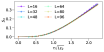
Figure 4: Rényi entropy of half chain in the short filter time. The data shows a good collapse of $S_{2}$ against $\tau\sqrt{L\varepsilon_{2}}$ for various system sizes, and compatibility with the universal prediction (39), black dashed line, is found.

We now discuss the analytic continuation of Eq. (38) to non-integer values of $n$. We need the following trigonometric equality (see e.g. Appendix A3 of Ref. [40])

$$\prod^{n-1}_{p=0}\left(x-\cos\frac{2\pi p}{n}y\right)=\left(\left(\frac{x+\sqrt{x^{2}-y^{2}}}{2}\right)^{n/2}-\left(\frac{x-\sqrt{x^{2}-y^{2}}}{2}\right)^{n/2}\right)^{2},$$ (40)

and we express Eq. (38) as

$$\text{det}\left(\mathbf{M}_{n}\right)=\left(\left(\frac{x+\sqrt{x^{2}-y^{2}}}{2}\right)^{n/2}-\left(\frac{x-\sqrt{x^{2}-y^{2}}}{2}\right)^{n/2}\right)^{2},$$ (41)

with

$$\begin{cases}x=\left(\frac{2}{\tilde{\tau}^{2}}+\varepsilon_{2}\right)^{2}-\varepsilon_{2}^{2}\left((1-V_{A}/V)^{2}+(V_{A}/V)^{2}\right),\\ y=2\varepsilon^{2}_{2}V_{A}/V(1-V_{A}/V).\end{cases}$$ (42)

From (41), one computes the Rényi entropies for non-integers values of $n$. We emphasize that the general logarithmic growth found in Eq. (20) for integer $n\geq 2$ as a function of $\tilde{\tau}$ is also present for $n\rightarrow 1$ and $n<1$. This mechanism has to be contrasted with the drastic change of behaviour observed in the medium filter time as $n$ crosses the value $1$, discussed at the end of Sec. A.

Appendix C Numerical methods

In this Section, we present (i) some further details on the numerical simulation that we discussed in the main text, and (ii) some additional numerical simulations that we performed in order to ensure the reliability of our results. We recall that our study focuses on the Ising model in Eq. (12); the initial state is the Néel state $\ket{\uparrow\downarrow\uparrow\downarrow\ldots\uparrow\downarrow}$, characterized by a vanishing energy density in the middle of the spectrum and an extensive energy variance.

Our numerical simulations are based on matrix-product states (MPS), a class of many-body quantum states that are characterized by a limited entanglement entropy and that display finite correlations decaying asymptotically exponentially in space in large enough one-dimensional systems [24]. The crucial parameter of MPS is the so-called bond link $\chi$: for $\chi=1$ MPS are product states, whereas for increasing $\chi$ they can accommodate for larger correlations and eventually, for large enough $\chi$, MPS can cover the entire Hilbert space of a finite-length quantum spin chain. MPS are a crucial tool for the numerical simulation of one-dimensional quantum many-body systems since for most situations of interest it is possible to accurately describe the quantum state with a limited value of $\chi$ and thus at a tractable numerical complexity.

The numerical simulation of an energy-filtered quantum state is complicated by the fact that while $H$ is a local Hamiltonian, the operator $H^{2}$ is non-local, and standard techniques such as TEBD or tDMRG [41, 42, 43, 44, 45] cannot be straightforwardly employed. For this reason, we use the Time-Dependent Variational Principle (TDVP) to implement the energy filter protocol [28, 29, 30] employing the ITensors library [31, 32]. In general, a TDVP is a scheme that projects the Schrödinger equation dictating the time-evolution of the state onto the manifold of MPS with fixed maximum bond link $\chi_{\rm max}$. The projection scheme can be done in several ways, and in particular allowing for the modification of only one site of the MPS (1-TDVP, first introduced in Ref. [29]) or of two neighboring sites (2-TDVP, first introduced in Ref. [30]). In general, the 1-TDVP suffers from the problem that it is not possible to increase the bond-link of the initial state during the time evolution, and thus requires an initial state represented by a sufficiently large bond-link in order to be able to describe the time-evolved state. The 2-TDVP algorithm does not suffer from this difficulty, but requires in turn a more important computational complexity. Following Ref. [33], we first apply the 2-TDVP and we evolve the initial state in time until a user-defined bond dimension is reached. Subsequently, we employ the 1-TDVP algorithm. This approach is a compromise between the computational efficiency, in terms of RAM and processing time, offered by 1-TDVP, and the mitigation of projection errors inherent in 2-TDVP, thereby enabling us to reach large filter time $\tau$ even for $L=80$ (see Ref. [33]). This is the technique employed to obtain the results presented in the main text, where the maximal bond link is $\chi=450$, the $\delta\tau=0.01$ and $[J,h_{x},h_{z}]=[1,1.2,0.8]$.

In order to probe the reliability of the TDVP algorithm, we have also performed simulations based on a straightforward expansion of the evolution operator, which is less efficient in terms of computational resources and time-step errors. This expansion is given by

$$\exp\left(-\frac{H^{2}\tau^{2}}{4}\right)=\left[\exp\left(-H^{2}\frac{\delta\tau^{2}}{4}\right)\right]^{N}\simeq\left(\mathds{1}-H^{2}\frac{\delta\tau^{2}}{4}\right)^{N},$$ (43)

with $\tau=\sqrt{N}\delta\tau$ (valid in the large $N$ limit). Since the Hamiltonian $H$ has a simple MPO representation, the MPO representation of $H^{2}$ follows automatically, and thus the operator $\mathds{1}-\frac{\delta\tau^{2}}{4}H^{2}$ can be contracted onto an MPS with standard techniques; we set the cutoff to $10^{-10}$ for the contraction between the MPO and the MPS, and to $0$ for the construction of the MPOs. Using this method we have been able to study spin chains up to $L=40$ and thus to produce numerical data to validate the TDVP data. We use $\delta\tau=0.05$ for $L=8,16,24$ and $\delta\tau=0.1$ for $L=32,40$.

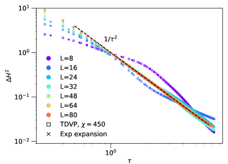
Figure 5: Energy variance $\Delta H^{2}$ as a function of $\tau$ for different system sizes. We have employed both the TDVP algorithm (bond dimension reached $\chi=450$, square markers) and the expansion (43) (crosses, for $L=8,16,24$), for $\delta\tau=0.1$. These methods are compatible, and they further show a collapse to $\Delta H^{2}=\tau^{-2}$ at large $L$.

In Fig. 5 we plot several data for the energy variance of the model obtained with both techniques for $L$ up to $80$. The agreement of the two techniques is excellent up to $L=24$ and with small differences at $\tau>5$ for $L=32,40$; for larger system size we could not produce data with the expansion in Eq. (43). For large $L$, we compare our numerics with the analytical prediction, since in the large $L$ limit we know that as the filter time $\tau$ increases, it should decrease as $\Delta H^{2}\simeq\tau^{-2}$. A collapse to this asymptotic scaling is observed for larger values of $L\sim 64,80$, while clear finite size effects are present for $L=8,16$. In this manner, we validate the results for both short and large $L$ obtained with the TDVP algorithm.

References

- Bañuls et al. [2020] M. C. Bañuls, D. A. Huse, and J. I. Cirac, Entanglement and its relation to energy variance for local one-dimensional hamiltonians, Phys. Rev. B 101, 144305 (2020).
- Rai et al. [2023] K. S. Rai, J. I. Cirac, and Á. M. Alhambra, Matrix product state approximations to quantum states of low energy variance, arXiv preprint arXiv:2307.05200 (2023).
- Lu et al. [2021] S. Lu, M. C. Banuls, and J. I. Cirac, Algorithms for quantum simulation at finite energies, PRX Quantum 2, 020321 (2021).
- Çakan et al. [2021] A. Çakan, J. I. Cirac, and M. C. Bañuls, Approximating the long time average of the density operator: Diagonal ensemble, Physical Review B 103, 115113 (2021).
- Luo et al. [2023] M. Luo, R. Trivedi, M. C. Bañuls, and J. I. Cirac, Probing off-diagonal eigenstate thermalization with tensor networks, arXiv preprint arXiv:2312.00736 (2023).
- Irmejs et al. [2023] R. Irmejs, M. C. Bañuls, and J. I. Cirac, Efficient quantum algorithm for filtering product states, arXiv preprint arXiv:2312.13892 (2023).
- Lu et al. [2024] S. Lu, G. Giudice, and J. I. Cirac, Variational neural and tensor network approximations of thermal states, arXiv preprint arXiv:2401.14243 (2024).
- Hartmann et al. [2004] M. Hartmann, G. Mahler, and O. Hess, Gaussian quantum fluctuations in interacting many particle systems, Lett. in Math. Phys. 68, 103 (2004).
- Lerose and Pappalardi [2020] A. Lerose and S. Pappalardi, Origin of the slow growth of entanglement entropy in long-range interacting spin systems, Phys. Rev. Res. 2, 012041 (2020).
- Pappalardi et al. [2018] S. Pappalardi, A. Russomanno, B. Žunkovič, F. Iemini, A. Silva, and R. Fazio, Scrambling and entanglement spreading in long-range spin chains, Phys. Rev. B 98, 134303 (2018).
- Schrodi et al. [2017] F. Schrodi, P. Silvi, F. Tschirsich, R. Fazio, and S. Montangero, Density of states of many-body quantum systems from tensor networks, Phys. Rev. B 96, 094303 (2017).
- Osborne [2006] T. J. Osborne, A renormalisation-group algorithm for eigenvalue density functions of interacting quantum systems, arXiv preprint cond-mat/0605194 (2006).
- Note [1] We refer to operators acting on a finite number of sites, and limits of their sequences in the operator norm. The interested reader can find a precise definition in Refs. [34, 35].
- Note [2] This asymptotic behavior comes from the extensivity of the cumulants of in the large volume limit.
- Heyl et al. [2013] M. Heyl, A. Polkovnikov, and S. Kehrein, Dynamical quantum phase transitions in the transverse-field ising model, Physical review letters 110, 135704 (2013).
- Pozsgay [2013] B. Pozsgay, The dynamical free energy and the loschmidt echo for a class of quantum quenches in the heisenberg spin chain, Journal of Statistical Mechanics: Theory and Experiment 2013, P10028 (2013).
- Fagotti [2019] M. Fagotti, On the size of the space spanned by a nonequilibrium state in a quantum spin lattice system, SciPost Phys. 6, 059 (2019).
- Calabrese and Cardy [2004] P. Calabrese and J. L. Cardy, Entanglement entropy and quantum field theory, J. Stat. Mech. 0406, P06002 (2004), arXiv:hep-th/0405152 .
- Calabrese and Cardy [2009] P. Calabrese and J. Cardy, Entanglement entropy and conformal field theory, Journal of Phys. A: Math. Phys. 42, 504005 (2009).
- Castro-Alvaredo and Doyon [2011] O. A. Castro-Alvaredo and B. Doyon, Permutation operators, entanglement entropy, and the XXZ spin chain in the limit , Journal of Statistical Mechanics: Theory and Experiment 2011, P02001 (2011).
- Hung et al. [2014] L.-Y. Hung, R. C. Myers, and M. Smolkin, Twist operators in higher dimensions, JHEP (10), 178, arXiv:1407.6429 [hep-th] .
- Foligno et al. [2023] A. Foligno, T. Zhou, and B. Bertini, Temporal entanglement in chaotic quantum circuits, Phys. Rev. X 13, 041008 (2023).
- Rakovszky et al. [2019] T. Rakovszky, F. Pollmann, and C. Von Keyserlingk, Sub-ballistic growth of rényi entropies due to diffusion, Physical review letters 122, 250602 (2019).
- Cirac et al. [2021] J. I. Cirac, D. Pérez-García, N. Schuch, and F. Verstraete, Matrix product states and projected entangled pair states: Concepts, symmetries, theorems, Rev. Mod. Phys. 93, 045003 (2021).
- Gotta et al. [2023] L. Gotta, S. Moudgalya, and L. Mazza, Asymptotic quantum many-body scars, Phys. Rev. Lett. 131, 190401 (2023).
- Furukawa et al. [2009] S. Furukawa, V. Pasquier, and J. Shiraishi, Mutual information and boson radius in a critical system in one dimension, Phys. Rev. Lett. 102, 170602 (2009).
- Desaules et al. [2022] J.-Y. Desaules, F. Pietracaprina, Z. Papić, J. Goold, and S. Pappalardi, Extensive multipartite entanglement from su(2) quantum many-body scars, Phys. Rev. Lett. 129, 020601 (2022).
- Paeckel et al. [2019] S. Paeckel, T. Köhler, A. Swoboda, S. R. Manmana, U. Schollwöck, and C. Hubig, Time-evolution methods for matrix-product states, Annals of Physics 411, 167998 (2019).
- Haegeman et al. [2011] J. Haegeman, J. I. Cirac, T. J. Osborne, I. Pižorn, H. Verschelde, and F. Verstraete, Time-dependent variational principle for quantum lattices, Phys. Rev. Lett. 107, 070601 (2011).
- Haegeman et al. [2016] J. Haegeman, C. Lubich, I. Oseledets, B. Vandereycken, and F. Verstraete, Unifying time evolution and optimization with matrix product states, Phys. Rev. B 94, 165116 (2016).
- Fishman et al. [2022a] M. Fishman, S. R. White, and E. M. Stoudenmire, The ITensor Software Library for Tensor Network Calculations, SciPost Phys. , 4 (2022a).
- Fishman et al. [2022b] M. Fishman, S. R. White, and E. M. Stoudenmire, Codebase release 0.3 for ITensor, SciPost Phys. Codebases , 4 (2022b).
- Goto and Danshita [2019] S. Goto and I. Danshita, Performance of the time-dependent variational principle for matrix product states in the long-time evolution of a pure state, Phys. Rev. B 99, 054307 (2019).
- Robinson [1967] D. W. Robinson, Statistical mechanics of quantum spin systems, Communications in Mathematical Physics 6, 151 (1967).
- Bratteli and Robinson [1987] O. Bratteli and D. Robinson, Operator algebras and quantum statistical mechanics 1, Bull. Amer. Math. Soc (1987).
- Calabrese and Cardy [2005] P. Calabrese and J. L. Cardy, Evolution of entanglement entropy in one-dimensional systems, J. Stat. Mech. 0504, P04010 (2005), arXiv:cond-mat/0503393 .
- Zhou and Nahum [2020] T. Zhou and A. Nahum, Entanglement membrane in chaotic many-body systems, Phys. Rev. X 10, 031066 (2020).
- Casini et al. [2016] H. Casini, H. Liu, and M. Mezei, Spread of entanglement and causality, JHEP 07, 077, arXiv:1509.05044 [hep-th] .
- Note [3] While (26) is derived within the hypothesis of fixed, it also holds in the limit . One can show it via a careful analysis of the spectrum of , reported in Eq. (24), in the limit above.
- Capizzi et al. [2022] L. Capizzi, S. Murciano, and P. Calabrese, Rényi entropy and negativity for massless complex boson at conformal interfaces and junctions, JHEP (11), 105, arXiv:2208.14118 [hep-th] .
- Schollwöck [2011] U. Schollwöck, The density-matrix renormalization group in the age of matrix product states, Annals of Physics 326, 96 (2011).
- Vidal [2003] G. Vidal, Efficient classical simulation of slightly entangled quantum computations, Phys. Rev. Lett. 91, 147902 (2003).
- Vidal [2004] G. Vidal, Efficient simulation of one-dimensional quantum many-body systems, Phys. Rev. Lett. 93, 040502 (2004).
- White and Feiguin [2004] S. R. White and A. E. Feiguin, Real-time evolution using the density matrix renormalization group, Phys. Rev. Lett. 93, 076401 (2004).
- Daley et al. [2004] A. J. Daley, C. Kollath, U. Schollwöck, and G. Vidal, Time-dependent density-matrix renormalization-group using adaptive effective hilbert spaces, Journal of Statistical Mechanics: Theory and Experiment 2004, P04005 (2004).