Multipath-based SLAM with Cooperation and Map Fusion
in MIMO Systems

Abstract

Multipath-based simultaneous localization and mapping (MP-SLAM) is a promising approach in wireless networks for obtaining position information of transmitters and receivers as well as information on the propagation environment. MP-SLAM models specular reflections of radio frequency (RF) signals at flat surfaces as virtual anchors (VAs), the mirror images of base stations. Conventional methods for MP-SLAM consider a single mobile terminal (MT) which has to be localized. The availability of additional MTs paves the way for utilizing additional information in the scenario. Specifically enabling MTs to exchange information allows for data fusion over different observations of VAs made by different MTs. Furthermore, cooperative localization becomes possible in addition to multipath-based localization. Utilizing this additional information enables more robust mapping and higher localization accuracy.

I Introduction

MP-SLAM is a powerful approach in wireless networks for obtaining position information of transmitters and receivers as well as information on the propagation environment. MP-SLAM models specular reflections of RF signals at flat surfaces as virtual anchors (VAs), the mirror images of BSs as shown in Fig. 1 [1]. MP-SLAM can detect and localize VAs and jointly estimate the time-varying MT position [1, 2, 3, 4, 5]. The availability of VA location information makes it possible to leverage multiple propagation paths of RF signals for MT localization, thus significantly improving localization accuracy and robustness [6, 7, 8, 9].

I-A State of the Art

MP-SLAM is a feature-based SLAM approach that focuses on detecting and mapping distinct features in the environment [10, 11, 12]. Features of interest are often referred to as VAs[3, 4, 5, 13] and ‘measurements” are obtained by extracting parameters from the multipath components of RF signals using a parametric channel estimation algorithm [14, 15, 16]. A complicating factor in MP-SLAM is measurement-origin uncertainty, i.e., the unknown association of measurements with features and their time-varying and unknown number[3, 4, 5, 17]. State-of-the-art methods consider these challenges in their joint statistical model. In particular, [3, 4, 5] use PDA and perform the sum-product algorithm (SPA) on a factor graph representing the underlying statistical model. Most of these methods rely on sampling techniques since the models for the aforementioned measurements are nonlinear [1, 6, 2, 3, 4, 5]. Recently, MP-SLAM was applied to data collected in indoor scenarios by radios with ultra-wide bandwidth or multiple antennas [2, 4]. In [18, 19], a method was developed to deal with non-ideal surfaces leading to possibly multiple reflections per VA. In [20] a novel MP-SLAM method is proposed that performs data fusion across multiple propagation path considering single-bounce and double-bounce reflections. Similar approaches were proposed in [21, 22] for simulaneous localization and tracking.

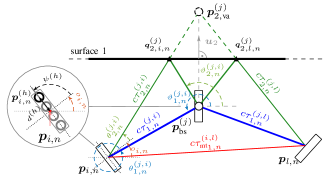
Figure 1: Exemplary indoor environment including a BS at position $\bm{p}^{(j)}_{\text{bs}}$ and two MTs at position $\bm{p}_{k,n}$, sharing information about a VA at position $\bm{p}^{(j)}_{l,\text{va}}$. A visualization of the array geometry definition used at the agent and PAs is included.

I-B Contributions

In this paper, we introduce a Bayesian particle-based SPA for cooperative MP-SLAM based on a factor graph that enables data fusion over different observations of map features (VAs) by different MTs as well as cooperative MT-to-MT measurements using RF signals. Our algorithm jointly performs PDA and sequential estimation of the states of the MTs and of potential s characterizing the map. The resulting SPA can infer VAs by combining information across multiple MTs for each BS. Furthermore, by considering MT-to-MT RF signals, the SPAs performs cooperative localization using PDA. In [23] a similar approach was proposed based on the probability hypothesis density filter with a different map fusion scheme. The key contributions are as follows.

• We model the exchange of information between different MTs, allowing for cooperative localization and data fusion of VAs over different MTs [20, 24].

• We fully integrate an inertial measurement unit (IMU) as an additional sensor for each MT. This unlocks additional information for orientation and state transition estimation allowing to cope with complex trajectories.

• We analyze the impact of VA data fusion and cooperative measurements in MP-SLAM for multiple input multiple output (MIMO) and single input multiple output (SIMO) systems using numerical simulation. In addition, we present the impact of using an IMU for the aforementioned cases.

Note that random variables are displayed in sans serif, upright fonts; their realizations in serif, italic fonts.

II Geometrical Relations

At time step $n$, we consider $I$ MTs with unknown state $\bm{x}_{i,n}=[\bm{p}_{i,n}\hskip 2.84526pt\bm{v}_{i,n}\hskip 2.84526pt\bm{o}_{i,n}]^{\text{T}}$ at positions $\bm{p}_{i,n}=[p_{x,i,n}\hskip 2.84526ptp_{y,i,n}]^{\text{T}}$ moving with velocity $\bm{v}_{i,n}=[v_{x,i,n}\hskip 2.84526ptv_{y,i,n}]^{\text{T}}$ in the direction of $o_{i,n}$ where $i\in\{1,\dots,I\}$ and $J$ BSs with known positions $\bm{p}_{1,\text{va}}^{(j)}\triangleq\bm{p}_{\mathrm{bs}}^{(j)},j\in\{1,\dots,J\}$. Each BS $j$ has $N_{n}^{(j)}-1$ specular reflections of radio signals at flat surfaces associated to it, modeled by VAs with unknown positions $\bm{p}_{l,\mathrm{va}}^{(j)}=\big{[}{p}_{x,l,\mathrm{va}}^{(j)}\hskip 0.85358pt\hskip 0.85358pt\hskip 0.85358pt{p}_{y,l,\mathrm{va}}^{(j)}\big{]}^{\mathrm{T}},l\in\{2,\dots,N_{n}^{(j)}\}$ (see [20]). By applying the image-source model [25, 20], a VA associated with a single-bounce path is the mirror image of $\bm{p}_{\mathrm{bs}}^{(j)}$ at reflective surface $l$ given by

$$\bm{p}^{(j)}_{l,\mathrm{va}} =\bm{p}^{(j)}_{\mathrm{bs}}+2\big{(}\bm{u}_{l}^{\text{T}}\bm{e}_{l}-\bm{u}_{l}^{\text{T}}\bm{p}^{(j)}_{\mathrm{bs}}\big{)}\bm{u}_{l}$$ (1)

where $\bm{u}_{l}$ is the normal vector of reflective surface $l$, and $\bm{e}_{l}$ is an arbitrary point on the considered surface. The according point of reflection $\bm{q}_{l,i,n}^{(j)}$ at the surface is given as

$$\bm{q}_{l,i,n}^{(j)}=\bm{p}_{l,\text{va}}^{(j)}+\frac{(\bm{p}_{\text{bs}}^{(j)}-\bm{p}_{l,\text{va}}^{(j)})^{\text{T}}\bm{u}_{l}}{2(\bm{p}_{i,n}-\bm{p}_{l,\text{va}}^{(j)})^{\text{T}}\bm{u}_{l}}(\bm{p}_{i,n}-\bm{p}_{l,\text{va}}^{(j)})$$ (2)

and is needed to relate angle-of-departure (AOD) of a specular reflection to the corresponding VA. Both the MTs and all BSs are equipped with antenna arrays. The geometry of an antenna array is represented by its array element positions, which are defined for the BSs arrays by the distances $d^{(j,h)}$ and the angles $\psi^{(j,h)}$ relative to the BS position $\bm{p}_{\mathrm{bs}}^{(j)}$ (with known orientation $o_{\text{bs}}^{(j)}$), and for MT array by distance $d^{(h)}$ and angle $\psi^{(h)}$ relative to the MT position $\bm{p}_{i,n}$ and unknown orientation $o_{i,n}$. The radio signal (see Appendix A) arrives at the receiver via the LOS path as well as via MPCs originating from the reflection of surrounding objects. The geometric relations of the MPCs parameters delay, angle-of-arrival (AOA) and AOD w.r.t. MT $i$ and PVA $j$ are respectively given by ${\tau_{\text{bs}}}_{l,n}^{(j,i)}\triangleq d(\bm{p}_{i,n},\bm{p}_{l,\text{va}}^{(j)})/c=\|\bm{p}_{i,n}\!-\bm{p}_{l,\text{va}}^{(j)}\|/c$, $\theta^{(j,i)}_{l,n}\triangleq\angle(\bm{p}_{i,n},\bm{p}_{l,\text{va}}^{(j)})$ with $\angle(\bm{p}_{i,n},\bm{p}_{l,\text{va}}^{(j)})=\text{atan2}\big{(}p_{y,l,\text{va}}^{(j)}-p_{y,i,n},p_{x,l,\text{va}}^{(j)}-p_{x,i,n})$ and $\vartheta^{(j,i)}_{l,n}\triangleq\angle(\bm{p}_{1,\text{va}}^{(j)},\bm{p}_{i,n})$ for $l=1$ and $\vartheta^{(j,i)}_{l,n}\triangleq\angle(\bm{q}_{l,i,n}^{(j)},\bm{p}_{i,n})$ for $l>1$ (see Fig. 1).

III Parametric Channel Estimation: Measurements

By applying at each time $n$, a channel estimation and detection algorithm (CEDA) [14, 15, 16] to the full observed discrete signal vector $\bm{r}_{\text{bs}_{n}}^{(j,i)}$ or $\bm{r}_{\text{mt}_{n}}^{(j,i)}$ (for details see Appendix A) of all antenna elements at MT $i$ and PA $j$ or MT $j$, one obtains a number of $M_{n}^{(j,i)}$ measurements denoted by ${\bm{z}^{(j,i)}_{m,n}}$ with $m\in{\cal{M}}_{n}^{(j)}\triangleq\{1,\,\dots\,,M_{n}^{(j)}\}$. Each $\bm{z}^{(j,i)}_{m,n}=[z^{(j,i)}_{\text{d}_{m,n}}\ z^{(j,i)}_{\theta_{m,n}}\ z^{(j,i)}_{\vartheta_{m,n}}\ z^{(j,i)}_{\mathrm{u}_{m,n}}]^{\text{T}}$ representing a potential MPC parameter estimate, contains a delay measurement $z^{(j,i)}_{\text{d}_{m,n}}\in[0,\tau_{\text{max}}]$, an AOA measurement $z^{(j,i)}_{\theta_{m,n}}\in[-\pi,\pi]$, an AOD measurement $z^{(j,i)}_{\vartheta_{m,n}}\in[-\pi,\pi]$ and a normalized amplitude measurement $z^{(j,i)}_{\mathrm{u}_{m,n}}\in[\gamma,\infty)$, where $\gamma$ is the detection threshold. Hence the CEDA compresses the information contained in $\bm{r}_{n}^{(j,i)}$ into $\vspace*{-1mm}\bm{z}^{(j,i)}_{n}=[{\bm{z}^{(j,i)\text{T}}_{1,n}}\cdots{\bm{z}^{(j,i)\text{T}}_{M_{n}^{(j,i)},n}}]^{\text{T}}$ which is used by the proposed algorithm as a noisy measurement.

IV System Model

At each time $n$, the states of the MTs are given by $\bm{\mathsfbr{x}}_{i,n}=[\bm{\mathsfbr{p}}_{i,n}^{\text{T}}\hskip 0.85358pt\bm{\mathsfbr{v}}_{i,n}^{\text{T}}\hskip 0.85358pt\bm{\mathsfbr{o}}_{i,n}]$, where $\bm{\mathsfbr{v}}_{i,n}$ are the MT velocities and $\bm{\mathsfbr{o}}_{i,n}$ are the orientations. As in [26, 3, 20], we account for the unknown number of VAs by introducing potential s (PVAs) $k\in\mathcal{K}^{(j)}_{n}\triangleq\{1,\dots,\mathsfbr{K}_{n}^{(j)}\}$. The number $\mathsfbr{K}_{n}^{(j)}$ of PVAs for each BS $j$ is the maximum possible number of actual VAs, i.e., all VAs that produced a measurement so far [26, 3, 20] (where $\mathsfbr{K}_{n}^{(j)}$ increases with time). The states of the PVAs are given by $\bm{\mathsfbr{y}}_{k,n}^{(j)}=\big{[}\bm{\mathsfbr{p}}^{(j)\hskip 0.85358pt\text{T}}_{k,\text{va}}\;\mathsfbr{u}^{(j)}_{k,n}\;\mathsfbr{r}^{(j)}_{k,n}\big{]}^{\text{T}}=\big{[}{\bm{\mathsfbr{x}}}^{(j)\hskip 0.85358pt\text{T}}_{k,n}\;\mathsfbr{r}^{(j)}_{k,n}\big{]}^{\text{T}}$, where $\mathsfbr{u}^{(j)}_{k,n}$ represents the normalized amplitude state of PVA $k$. The existence/nonexistence of PVAs $k$ is modeled by the existence variable $\mathsfbr{r}_{k,n}^{(j)}\in\{0,1\}$ in the sense that PVAs exists if $r_{k,n}^{(j)}=1$. Formally, its states is considered even if PVAs $k$ is nonexistent, i.e., if $r_{k,n}^{(j)}=0$. The states ${\bm{\mathsfbr{x}}}^{(j)}_{k,n}$ of nonexistent PVAs are irrelevant, hence probability density functions defined for PVA states are of the form $f({\bm{x}}^{(j)}_{k,n},0)=f^{(j)}_{k,n}f_{\text{d}}({\bm{x}}^{(j)}_{k,n})$, where $f_{\text{d}}({\bm{x}}^{(j)}_{k,n})$ is an arbitrary “dummy PDF” and $f^{(j)}_{k,n}\!\in[0,1]$ is a constant and can be interpreted as the probability of non-existence [26, 3].

IV-A BS-MT Measurement Model and New PVAs

An existing PVA generates a measurement ${\bm{\mathsfbr{z}}_{\text{bs}}}^{(j,i)}_{m,n}$ with $m\in{\mathcal{M}_{\text{bs}}}^{(j,i)}_{n}\triangleq\{1,\dots,{\mathsfbr{M}_{\text{bs}}}^{(j,i)}_{n}\}$ with detection probability ${p_{\mathrm{d}}}(\mathsfbr{u}^{(j)}_{k,n})$. The single measurement likelihood function (LHF) is given by $f({\bm{z}_{\text{bs}}}^{(j,i)}_{m,n}|\bm{x}_{i,n},\bm{y}^{(j)}_{k,n})$, and it is assumed to be conditionally independent across the individual measurements within the vector ${\bm{\mathsfbr{z}}_{\text{bs}}}^{(j,i)}_{m,n}$, thus it factorizes as

$$f({\bm{z}_{\text{bs}}}^{(j,i)}_{m,n}|\bm{x}^{(j)}_{k,n},\bm{x}_{i,n}) =f(z^{(j,i)}_{\text{d}_{m,n}}|\bm{p}_{i,n},\bm{x}^{(j)}_{k,n})f(z^{(j,i)}_{\mathrm{u}_{m,n}}|u^{(j)}_{k,n})$$

$$\times f(z^{(j,i)}_{\theta_{m,n}}|\bm{x}_{i,n},\bm{x}^{(j)}_{k,n})f(z^{(j,i)}_{\vartheta_{m,n}}|\bm{p}_{i,n},\bm{x}^{(j)}_{k,n})$$ (3)

where the individual LHFs of the distance, AOA and AOD measurements are modeled by Gaussian PDFs $f_{\mathrm{N}}(x;\mu,\sigma^{2})$ [27]. More specifically, the LHF of the distance measurement is given by

$$f(z^{(j,i)}_{\text{d}_{m,n}}|\bm{p}_{i,n},\bm{x}^{(j)}_{k,n})=f_{\mathrm{N}}(z^{(j,i)}_{\text{d}_{m,n}};d(\bm{p}_{i,n},\bm{p}^{(j)}_{k,\text{va}}),\sigma_{\mathrm{d}}^{2}(u^{(j)}_{k,n}))$$ (4)

where $\sigma_{\mathrm{d}}^{2}({u}^{(j)}_{k,n})=c^{2}/(8\pi^{2}\beta_{\mathrm{bw}}^{2}{u}_{k,n}^{(j)\hskip 0.85358pt2})$ is determined based on the Fisher information with $\beta_{\mathrm{bw}}^{2}$ denoting the mean square bandwidth of $S^{(j)}_{\text{bs}}(f)$ [28, 7, 9, 29]. The LHF of the AOA and AOD measurements are given by

$$f(z^{(j,i)}_{\theta_{m,n}}|\bm{x}_{i,n},\bm{x}^{(j)}_{k,n})$$

$$=f_{\mathrm{N}}(z^{(j,i)}_{\theta_{m,n}};\angle(\bm{p}_{i,n},\bm{p}^{(j)}_{k,\text{va}})-o_{i,n},\sigma_{\theta}^{2}(u^{(j)}_{k,n}))$$ (5)

$$f(z^{(j,i)}_{\vartheta_{m,n}}|\bm{p}_{i,n},\bm{x}^{(j)}_{k,n})$$

$$=f_{\mathrm{N}}(z^{(j,i)}_{\vartheta_{m,n}};\angle(\bm{p}_{i,n},\bm{p}^{(j)}_{k,\text{va}}),\sigma_{\vartheta}^{2}(u^{(j)}_{k,n}))$$ (6)

where $\sigma_{\mathrm{\theta}}^{2}({u}^{(j)}_{k,n})=1/\big{(}8\pi^{2}{u}^{(j)\hskip 0.85358pt2}_{k,n}D^{2}\big{(}\angle(\bm{p}_{i,n},\bm{p}^{(j)}_{k,\text{va}})-{o}_{i}\big{)}$ and $\sigma_{\mathrm{\vartheta}}^{2}({u}^{(j)}_{k,n})=1/\big{(}8\pi^{2}{u}^{(j)\hskip 0.85358pt2}_{k,n}D^{2}\big{(}\angle(\bm{p}^{(j)}_{k,\text{va}},\bm{p}_{i,n})\big{)}$ are determined based on the Fisher information with $D^{2}\big{(}\cdot\big{)}$ as normalized squared aperture of the antenna array [7, Equation (24)]. The LHF of the normalized amplitude measurements ${u}^{(j)}_{k,n}>\gamma$ is modeled by a truncated Rician PDF [30, Ch. 1.6.7], [17], i.e.,

$$f(z^{(j,i)}_{\mathrm{u}_{m,n}}|u^{(j)}_{k,n})=f_{\mathrm{TR}}(z^{(j,i)}_{\mathrm{u}_{m,n}};u^{(j)}_{k,n},\sigma_{\mathrm{u}}(u^{(j)}_{k,n}),{p_{\mathrm{d}}}(u^{(j)}_{k,n});\gamma)$$ (7)

where the scale parameter $\sigma_{\mathrm{u}}({u}^{(j)}_{k,n})$ is determined based on the Fisher information given as $\sigma_{\mathrm{u}}^{2}({u}^{(j)}_{k,n})=\frac{1}{2}+\frac{1}{4MH}{u}^{(j)\hskip 0.85358pt2}_{k,n}$. The variance $\sigma_{\mathrm{u}}^{2}({u}^{(j)}_{k,n})$ also considers for the measurement noise variance estimation of the CEDA (preprocessing) [17]. The ${p_{\mathrm{d}}}({u}^{(j)}_{k,n})$[31, 30, 17] is directly related to the PVA’s visibility and the detection threshold $u_{\text{de}}$ of the CEDA (preprocessing) is directly connected to the likelihood model of the proposed MP-SLAM (see [17]). False alarm (FA) measurements originating from the snapshot-based parametric channel estimator are assumed statistically independent of PVA states. These measurements are modeled by a Poisson process with mean number $\mu_{\mathrm{fa}}$ and PDF $f_{\mathrm{fa}}({\bm{z}_{\text{bs}}}^{(j,i)}_{m,n})$, which is factorized as $f_{\mathrm{fa}}({\bm{z}_{\text{bs}}}^{(j,i)}_{m,n})=f_{\mathrm{fa}}(z^{(j,i)}_{\text{d}_{m,n}})f_{\mathrm{fa}}(z^{(j,i)}_{\theta_{m,n}})f_{\mathrm{fa}}(z^{(j,i)}_{\vartheta_{m,n}})f_{\mathrm{fa}}(z^{(j,i)}_{\mathrm{u}_{m,n}})$. The FA LHFs of the measurements corresponding to distance, AOA and AOD are uniformly distributed on $[0,d_{\mathrm{max}}]$, $[-\pi,\pi)$ and $[-\pi,\pi)$, respectively. The FA LHF $f_{\mathrm{fa}}(z^{(j,i)}_{\mathrm{u}_{m,n}})$ of the normalized amplitude is given by a truncated Rayleigh PDF (see [17, 32] for details).

Newly detected VAs i.e., VAs that generated a measurement for the first time, are modeled by a Poisson process with mean $\mu_{\mathrm{n}}$ and PDF $f_{\mathrm{n}}(\overline{\bm{x}}^{(j,i)}_{m,n}|\bm{x}_{i,n})$. Newly detected VAs are represented by new PVA states $\overline{\bm{\mathsfbr{y}}}^{(j,i)}_{n,m}$, $m\in\{1,\dots,{\mathsfbr{M}_{\text{bs}}}^{(j,i)}_{n}\}$ in our statistical model [26, 3]. Each new PVA state corresponds to a measurement ${\bm{\mathsfbr{z}}_{\text{bs}}}^{(j,i)}_{m,n}$; $\overline{r}_{m,n}\!=\!1$ implies that measurement ${\bm{\mathsfbr{z}}_{\text{bs}}}^{(j,i)}_{m,n}$ was generated by a newly detected VA. We denote by $\overline{\bm{\mathsfbr{y}}}^{(j,i)}_{n}\triangleq\big{[}\hskip 0.85358pt\overline{\bm{\mathsfbr{y}}}^{(j,i)\hskip 0.85358pt\text{T}}_{1,n}\hskip 0.85358pt\cdots\hskip 0.85358pt\overline{\bm{\mathsfbr{y}}}^{(j,i)\hskip 0.85358pt\text{T}}_{{\mathsfbr{M}_{\text{bs}}}^{(j,i)}_{n},n}\hskip 0.85358pt\big{]}^{\text{T}}$, the joint vector of all new PVA states. Introducing new PVA for each measurement leads to a number of PVA states that grows with time $n$. Thus, to keep the proposed MP-SLAM algorithm feasible, a sub-optimum pruning step is performed, removing PVAs with a low probability of existence.

IV-B Legacy PVAs and Sequential Update

At time $n$, measurements are incorporated sequentially across MTs $i\in\{1,\dots,I\}$ [26, 20]. Previously detected VAs, i.e., VAs that have been detected either at a previous time $n^{\prime}\!<n$ or at the current time $n$ but at a previous MT $i^{\prime}\!<i$, are represented by legacy PVA states $\underline{\bm{\mathsfbr{y}}}_{k,n}^{(j)}$. New PVAs become legacy PVAs when the next measurements, either of the next MT or at the next time instance, are taken into account. In particular, the VA represented by the new VA state $\overline{\bm{\mathsfbr{y}}}^{(j,i^{\prime})}_{m^{\prime},n^{\prime}}$ introduced due to measurement $m^{\prime}$ of MT $i^{\prime}$ at time $n^{\prime}\leqslant n$ is represented by the legacy PVA state $\underline{\bm{\mathsfbr{y}}}^{(j)}_{k,n}$ at time $n$, with $k=\mathsfbr{K}^{(j)}_{n^{\prime}-1}+\sum^{i^{\prime}-1}_{i^{\prime\prime}=1}{\mathsfbr{M}_{\text{bs}}}^{(j,i^{\prime\prime})}_{n}+m^{\prime}$. The number of legacy PVA at time $n$, when the measurements of the next MT $i$ are incorporated, is updated according to $\mathsfbr{K}^{(j,i)}_{n}=\mathsfbr{K}^{(j,i-1)}_{n-1}+{\mathsfbr{M}_{\text{bs}}}^{(j,i-1)}_{n}$, where $\mathsfbr{K}^{(j,1)}_{n}=\mathsfbr{K}^{(j)}_{n-1}$. Here, $\mathsfbr{K}^{(j,i)}_{n}$ is equal to the number of all measurements collected up to time $n$ and MT $i-1$. The vector of all legacy PVA states at time $n$ and up to MT $i$ can now be written as $\underline{\bm{\mathsfbr{y}}}^{(j,i)}_{n}=\big{[}\underline{\bm{\mathsfbr{y}}}^{(j,i-1)\text{T}}_{n}\hskip 0.85358pt\hskip 0.85358pt\hskip 0.85358pt\overline{\bm{\mathsfbr{y}}}^{(j,i-1)\text{T}}_{n}\big{]}^{\text{T}}$ and the current vector containing all states as ${\bm{\mathsfbr{y}}}^{(j,i-1)}_{n}=\big{[}\underline{\bm{\mathsfbr{y}}}^{(j,i-1)\text{T}}_{n}\hskip 0.85358pt\hskip 0.85358pt\hskip 0.85358pt\overline{\bm{\mathsfbr{y}}}^{(j,i-1)\text{T}}_{n}\big{]}^{\text{T}}$ where $\underline{\bm{\mathsfbr{y}}}^{(j,1)}_{n}\triangleq\big{[}\underline{\bm{\mathsfbr{y}}}^{(j)\hskip 0.85358pt\text{T}}_{1,n}\cdots\hskip 0.85358pt\underline{\bm{\mathsfbr{y}}}^{(j)\hskip 0.85358pt\text{T}}_{\mathsfbr{K}^{(j)}_{n-1},n}\big{]}^{\text{T}}$ is the vector of all legacy PVA states before any measurements at time $n$ have been incorporated. After the measurements of all MTs $i\in\{1,\dots,I\}$ have been incorporated at time $n$, the total number of PVA states is $\mathsfbr{K}^{(j)}_{n}=\mathsfbr{K}^{(j)}_{n-1}+\sum_{i=1}^{I}{\mathsfbr{M}_{\text{bs}}}^{(j,i)}_{n}=\mathsfbr{K}^{(j,I)}_{n}+{\mathsfbr{M}_{\text{bs}}}^{(j,I)}_{n}$ and the vector of all PVA states at time $n$ is given by $\bm{\mathsfbr{y}}^{(j)}_{n}\!=\big{[}\underline{\bm{\mathsfbr{y}}}^{(j,I)\hskip 0.85358pt\text{T}}_{n}\hskip 0.85358pt\hskip 0.85358pt\overline{\bm{\mathsfbr{y}}}^{(j,I)\text{T}}_{n}\big{]}^{\text{T}}$.

IV-C State Evolution

Legacy PVAs states $\underline{\bm{\mathsfbr{y}}}^{(j)}_{k,n}$ and the MT states $\bm{\mathsfbr{x}}_{i,n}$ are assumed to evolve independently across time according to state-transition PDFs $f\big{(}\underline{\bm{y}}^{(j)}_{k,n}\big{|}\bm{y}_{k,n-1}\big{)}$ and $f(\bm{x}_{i,n}|\bm{x}_{i,n-1},\bm{c}_{i,n-1})$, respectively, where $\bm{c}_{i,n-1}$ is a control term. If PVA $k$ exists at time $n-\!1$, i.e., $r^{(j)}_{k,n-1}\!=\!1$, it either disappears, i.e., $\overline{r}^{(j)}_{k,n}\!=0$, or survives, i.e., $\overline{r}^{(j)}_{k,n}\!=\!1$; in the latter case, it becomes a legacy PVA at time $n$. The probability of survival is denoted by $p_{\mathrm{s}}$. In case of survival, its position remains unchanged, i.e., the state-transition PDF of the VA positions $\underline{\bm{\mathsfbr{p}}}^{(j)}_{k,\mathrm{va}}$ is given by $f\big{(}\underline{\bm{p}}^{(j)}_{k,\mathrm{va}}\hskip 0.85358pt\big{|}\hskip 0.85358pt\bm{p}^{(j)}_{k,\mathrm{va}}\big{)}=\delta\big{(}\underline{\bm{p}}^{(j)}_{k,\mathrm{va}}-\hskip 0.85358pt\bm{p}^{(j)}_{k,\mathrm{va}}\big{)}$ and for the normalized amplitude $\mathsfbr{u}^{(j)}_{k,n}$ is given by $f\big{(}\underline{u}^{(j)}_{k,n}\hskip 0.85358pt\big{|}\hskip 0.85358ptu^{(j)}_{k,n-1}\big{)}$. Therefore, $f\big{(}\underline{\bm{x}}^{(j)}_{k},\underline{r}^{(j)}_{k,n}\hskip 0.85358pt\big{|}\hskip 0.85358pt\bm{x}^{(j)}_{k},r^{(j)}_{k,n-1}\big{)}$ for $r^{(j)}_{k,n-1}=1$ is obtained as

$$f\big{(}\underline{\bm{x}}^{(j)}_{k},\underline{r}^{(j)}_{k,n}\hskip 0.85358pt\big{|}\hskip 0.85358pt\bm{x}^{(j)}_{k},r^{(j)}_{k,n-1}=1\big{)}$$

$$=\begin{cases}(1\!-p_{\mathrm{s}})\hskip 0.85358ptf_{\text{d}}\big{(}\underline{\bm{p}}^{(j)}_{k,\mathrm{va}}\big{)},&\!\!\!\underline{r}^{(j)}_{k,n}\!=0\\[0.0pt] p_{\mathrm{s}}\hskip 0.85358pt\hskip 0.85358ptf\big{(}\underline{u}^{(j)}_{k,n}\hskip 0.85358pt\big{|}\hskip 0.85358ptu^{(j)}_{k,n-1}\big{)}\delta\big{(}\underline{\bm{p}}^{(j)}_{k,\mathrm{va}}-\hskip 0.85358pt\bm{p}^{(j)}_{k,\mathrm{va}}\big{)},&\!\!\!\underline{r}^{(j)}_{k,n}\!=\!1.\end{cases}$$ (8)

If VA $k$ does not exist at time $n-\!1$, i.e., $r^{(j)}_{k,n-1}\!=\!0$, it cannot exist as a legacy PVA at time $n$ either, thus we get

$$f\big{(}\underline{\bm{x}}^{(j)}_{k},\underline{r}^{(j)}_{k,n}\big{|}\bm{x}^{(j)}_{k},r^{(j)}_{k,n-1}=0\big{)}=\begin{cases}f_{\text{d}}\big{(}\underline{\bm{x}}^{(j)}_{k}\big{)},&\!\!\!\underline{r}^{(j)}_{k,n}\!=0\\[0.0pt] 0,&\!\!\!\underline{r}^{(j)}_{k,n}\!=\!1.\end{cases}$$ (9)

For $i\geqslant 2$, we also define $f^{(i)}\big{(}\underline{\bm{y}}^{(j,i)}_{k,n}\big{|}{\bm{y}}^{(j,i-1)}_{k,n}\big{)}$ as

$$f^{(i)}\big{(}\underline{\bm{x}}^{(j,i)}_{k},\underline{r}^{(j,i)}_{k,n}\hskip 0.85358pt\big{|}{\hskip 0.85358pt{\bm{x}}^{(j,i-1)}_{k},{r}^{(j,i-1)}_{k,n}=1}\big{)}$$

$$=\begin{cases}f_{\text{d}}\big{(}\underline{\bm{x}}^{(j,i)}_{k}\big{)},&\!\!\!\underline{r}^{(j,i)}_{k,n}\!=0\\[0.0pt] \delta\big{(}\underline{\bm{x}}^{(j,i)}_{k}-\hskip 0.85358pt{\bm{x}}^{(j,i-1)}_{k}\big{)},&\!\!\!\underline{r}^{(j,i)}_{k,n}\!=\!1\end{cases}$$ (10)

and

$$f^{(i)}\big{(}\underline{\bm{x}}^{(j,i)}_{k},\underline{r}^{(j,i)}_{k,n}\big{|}{{\bm{x}}^{(j,i-1)}_{k},{r}^{(j,i-1)}_{k,n}=0}\big{)}$$

$$=\begin{cases}f_{\text{d}}\big{(}\underline{\bm{x}}^{(j,i)}_{k}\big{)},&\!\!\!\underline{r}^{(j,i)}_{k,n}\!=0\\[0.0pt] 0,&\!\!\!\underline{r}^{(j,i)}_{k,n}\!=\!1.\end{cases}$$ (11)

It it assumed that at time $n=0$ the initial prior PDF $f\big{(}\bm{y}^{(j)}_{k,0}\big{)}$, $k=\big{\{}1,\dots,K^{(j)}_{0}\big{\}}$ and $f(\bm{x}_{i,0})$ are known. All (legacy and new) PVA states and all MT states up to time $n$ are denoted as $\bm{\mathsfbr{y}}_{n}\!=\big{[}\bm{\mathsfbr{y}}^{(1)\hskip 0.85358pt\text{T}}_{n}\cdots\hskip 0.85358pt\bm{\mathsfbr{y}}^{(J)\text{T}}_{n}\big{]}^{\text{T}}$ and $\bm{\mathsfbr{y}}_{0:n}\triangleq\big{[}\bm{\mathsfbr{y}}^{\text{T}}_{0}\cdots\hskip 0.85358pt\bm{\mathsfbr{y}}^{\text{T}}_{n}\big{]}^{\text{T}}\!$ and $\bm{\mathsfbr{x}}_{n}=[\bm{\mathsfbr{x}}_{1,n}^{\text{T}}\hskip 0.85358pt\cdots\bm{\mathsfbr{x}}_{I_{\text{MT}},n}^{\text{T}}]$ and $\bm{\mathsfbr{x}}_{0:n}=[\bm{\mathsfbr{x}}_{0}^{\text{T}}\hskip 0.85358pt\cdots\bm{\mathsfbr{x}}_{n}^{\text{T}}]$, respectively.

IV-D MT-MT Measurement Model

An existing LOS between MT $i$ and MT $i^{\prime}$ generates a measurement ${\bm{\mathsfbr{z}}_{\text{co}}}^{(i,i^{\prime})}_{m,n}\in{\mathcal{M}_{\text{co}}}^{(i,i^{\prime})}_{n}\triangleq\{1,\dots,{\mathsfbr{M}_{\text{co}}}^{(j,i)}_{n}\}$. The single measurement LHF is given by $f({\bm{z}_{\text{co}}}^{(i,i^{\prime})}_{m,n}|\bm{x}_{i,n},\bm{x}_{i^{\prime},n})$, and it is assumed to be conditionally independent across the individual measurements within the vector ${\bm{\mathsfbr{z}}_{\text{co}}}^{(i,i^{\prime})}_{m,n}$. Since the orientation of both MTs is a nuisance parameter, the angular measurements do not provide additional information in that case. Hence, we only consider distance measurements and neglect angular measurements for cooperation. The LHFs is given as

$$f({\bm{z}_{\text{co}}}^{(i,i^{\prime})}_{m,n}|\bm{x}_{i,n},\bm{x}_{i^{\prime},n}) =f({z_{\mathrm{co,d}}}^{(i,i^{\prime})}_{m,n}|\bm{p}_{i,n},\bm{p}_{i^{\prime},n})$$ (12)

IV-E IMU Measurement Model

At each time step $n$, an IMU, consisting of an accelerometer, a gyroscope and a magnetometer, provides each MT with the corresponding IMU measurements $\bm{z}_{\text{acc}_{i,n}},\bm{z}_{\text{gyr}_{i,n}}$ and $\bm{z}_{\text{mag}_{i,n}}$, respectively. The normalized acceleration measurement is defined as $\tilde{\bm{z}}_{\text{acc}_{i,n}}=\bm{z}_{\text{acc}_{i,n}}/\|\bm{z}_{\text{acc}_{i,n}}\|$. Therefor, we define $\bm{z}_{\text{IMU}_{i,n}}=[\tilde{\bm{z}}_{\text{acc}_{i,n}}^{\text{T}}\bm{z}_{\text{gyr}_{i,n}}^{\text{T}}\tilde{\bm{z}}_{\text{mag}_{i,n}}^{\text{T}}]^{\text{T}}$. The IMU LHF is given as

$$f(\bm{z}_{\text{IMU}_{i,n}}|\bm{x}_{i,n^{\prime}}) =f_{\mathrm{N}}(\bm{z}_{\text{IMU}_{i,n}},\bm{o}_{i,n},\Sigma_{i})$$ (13)

where $\Sigma_{i}$ is a blockdiagonal covariance matrix. For the orientation state, a quaternion representation is used and the mapping of the IMU measurements to the quaternion state is done similarly to [33].

$$f\big{(}\bm{y}_{0:n},\bm{x}_{0:n},\underline{\bm{a}}_{1:n},\overline{\bm{a}}_{1:n},\bm{b}_{1:n}\hskip 0.85358pt\big{|}\hskip 0.85358pt\bm{z}_{1:n}\big{)} \propto\underbrace{\bigg{(}\prod^{I}_{i=1}\hskip 0.85358ptf(\bm{x}_{i,0})\hskip 0.85358pt\prod^{K_{0}}_{k=1}\hskip 0.85358ptf(\bm{y}_{k,0})\bigg{)}}_{\footnotesize\text{MT and VA states initial prior PDFs}}\prod^{n}_{n^{\prime}=1}\underbrace{\bigg{(}\prod^{I}_{i=1}\hskip 0.85358ptf\big{(}\bm{x}_{i,n^{\prime}}|\bm{x}_{i,n^{\prime}-1},\bm{c}_{i,n^{\prime}-1}\big{)}f\big{(}\bm{z}_{\text{IMU}_{i,n^{\prime}}}|\bm{x}_{i,n^{\prime}}\big{)}}_{\footnotesize\text{MT state prediction and IMU measurement}}$$

$$\times\underbrace{\prod^{I}_{i^{\prime}=1,i\neq i^{\prime}}\hskip 0.85358pt\hskip 0.85358ptg_{\text{co}}\big{(}\bm{x}_{i,n^{\prime}},\bm{x}_{i^{\prime},n^{\prime}},b^{(i,i^{\prime})}_{n^{\prime}};{\bm{z}_{\text{co}}}_{n^{\prime}}\big{)}\bigg{)}}_{\footnotesize\text{MT cooperative related factors}}\underbrace{\bigg{(}\prod^{J}_{j=1}\prod^{K^{(j)}_{n^{\prime}-1}}_{k^{\prime}=1}f\big{(}\underline{\bm{y}}^{(j)}_{k^{\prime},n^{\prime}}|\bm{y}^{(j)}_{k^{\prime},n^{\prime}-1}\big{)}\bigg{)}}_{\footnotesize\text{Legacy PVA states prediction}}\underbrace{\bigg{(}\prod^{J}_{j=1}\hskip 0.85358pt\prod^{I}_{i=2}\hskip 0.85358pt\prod^{K^{(j,i)}_{n^{\prime}}}_{k=1}\hskip 0.85358ptf^{(i)}\big{(}\underline{\bm{y}}^{(j,i)}_{k,n^{\prime}}\big{|}\underline{\bm{y}}^{(j,i-1)}_{k,n^{\prime}}\big{)}\bigg{)}}_{\footnotesize\text{Legacy PVA states transition factors}}$$

$$\times\underbrace{\prod^{J}_{j=1}\prod^{I}_{i=1}\prod^{K^{(i)}_{n^{\prime}}}_{k=1}\hskip 0.85358pt\underline{q}_{\text{BS}}\big{(}\underline{\bm{y}}^{(j,i)}_{k,n^{\prime}},\underline{a}^{(j,i)}_{k,n^{\prime}},\bm{x}_{i,n^{\prime}};{\bm{z}_{\text{bs}}}^{(j)}_{i,n^{\prime}}\big{)}\prod^{{M_{\text{bs}}}^{(j,i)}_{n^{\prime}}}_{m=1}\Psi\big{(}\underline{a}^{(j,i)}_{k,n^{\prime}},\overline{a}^{(j,i)}_{m,n^{\prime}}\big{)}}_{\footnotesize\text{Legacy PVA states related factors}}\underbrace{\prod^{{M_{\text{bs}}}^{(j,i)}_{n^{\prime}}}_{m=1}\overline{q}_{\text{BS}}\big{(}\overline{\bm{y}}^{(j,i)}_{m,n^{\prime}},\overline{a}^{(j,i)}_{m,n^{\prime}},\bm{x}_{n^{\prime}};{\bm{z}_{\text{bs}}}^{(j)}_{i,n^{\prime}}\big{)}}_{\footnotesize\text{New PVA states prior PDF and related factors}}$$ (14)

IV-F Data Association

The data association between MTs and MVAs as well as MTs and MTs is described in Appendix B.

IV-G Joint Posterior PDF and Factor Graph

Using Bayes’ rule and independence assumptions related to the state-transition PDFs, the prior PDFs, and the likelihood model (for details please see [26, 3, 20]), and for fixed (observed) measurements $\bm{z}_{1:n}$ (the numbers of measurements ${M_{\text{bs}}}^{(j,i)}_{n}$ and ${M_{\text{co}}}^{(i,i^{\prime})}_{n}$ are fixed and not random anymore) the joint posterior PDF of $\bm{\mathsfbr{y}}_{0:n}$, $\bm{\mathsfbr{x}}_{0:n}$, $\underline{\bm{\mathsfbr{a}}}_{1:n}$, $\overline{\bm{\mathsfbr{a}}}_{1:n}$ and $\bm{\mathsfbr{b}}_{1:n}$ conditioned on $\bm{z}_{1:n}$ is given by (14) where we introduced the functions $g_{\text{co}}\big{(}\bm{x}_{i,n},\bm{x}_{i^{\prime},n},b^{(i,i^{\prime})}_{n};{\bm{z}_{\text{co}}}^{(i,i^{\prime})}_{n}\big{)}$, $\underline{q}_{\text{BS}}\big{(}\underline{\bm{y}}^{(j,i)}_{k,n},\underline{a}^{(j,i)}_{k,n},\bm{x}_{i,n};{\bm{z}_{\text{bs}}}^{(j)}_{i,n}\big{)}$, and $\overline{q}_{\text{BS}}\big{(}\overline{\bm{y}}^{(j,i)}_{m,n},$ $\overline{a}^{(j,i)}_{m,n},\bm{x}_{i,n};{\bm{z}_{\text{bs}}}^{(j)}_{i,n}\big{)}$ that will be discussed next.

The pseudo likelihood functions $g_{\text{co}}\big{(}\bm{x}_{i,n},\bm{x}_{i^{\prime},n},b^{(i,i^{\prime})}_{n};{\bm{z}_{\text{co}}}_{n}\big{)}$ and $\underline{q}_{\text{BS}}\big{(}\underline{\bm{y}}^{(j,i)}_{k,n},\underline{a}^{(j,i)}_{k,n},\bm{x}_{i,n};{\bm{z}_{\text{bs}}}^{(j)}_{i,n}\big{)}$ are respectively given for $(i,i^{\prime})\in\mathcal{C}^{(i,^{\prime}i)}_{n}$ by

$$g_{\text{co}}\big{(}\bm{x}_{i,n},\bm{x}_{i^{\prime},n},b^{(i,i^{\prime})}_{n};{\bm{z}_{\text{co}}}^{(i,i^{\prime})}_{n}\big{)}$$

$$\triangleq\begin{cases}\displaystyle\hskip 0.85358pt\frac{p^{(j)}_{\mathrm{d}}(u_{i,n})f\big{(}{\bm{z}_{\text{co}}}^{(i,i^{\prime})}_{m,n}\big{|}\hskip 0.85358pt\bm{x}_{i,n},\bm{x}_{i^{\prime},n}\big{)}}{\mu_{\mathrm{fa}}\hskip 0.85358ptf_{\mathrm{fa}}\big{(}{\bm{z}_{\text{co}}}^{(i,i^{\prime})}_{m,n}\big{)}}\hskip 0.85358pt,&\!\!b^{(i,i^{\prime})}_{n}\!=m\in{{\cal{M}}_{\text{co}}}^{(i,i^{\prime})}_{n}\\[9.95845pt] 1\!-p^{(j)}_{\mathrm{d}}(\bm{p}_{i,n},\bm{p}_{i^{\prime},n})\hskip 0.85358pt,&\!\!b^{(i,i^{\prime})}_{n}\!=0\end{cases}$$ (15)

for BS $j$ and MT $i$ by

$$\underline{q}_{\text{BS}}\big{(}\underline{\bm{x}}^{(j,i)}_{k,n},\underline{r}^{(j,i)}_{k,n}=1,\underline{a}^{(j,i)}_{k,n},\bm{x}_{i,n};{\bm{z}_{\text{bs}}}^{(j,i)}_{n}\big{)}$$

$$\triangleq\begin{cases}\displaystyle\hskip 0.85358pt\frac{p^{(j)}_{\mathrm{d}}(\underline{u}^{(j,i)}_{k,n})f\big{(}{\bm{z}_{\text{bs}}}^{(j,i)}_{m,n}\big{|}\hskip 0.85358pt\bm{x}_{i,n},\underline{\bm{x}}^{(j,i)}_{k,n}\big{)}}{\mu_{\mathrm{fa}}\hskip 0.85358ptf_{\mathrm{fa}}\big{(}f\big{(}{\bm{z}_{\text{bs}}}^{(j,i)}_{m,n}\big{)}}\hskip 0.85358pt,&\!\!\underline{a}^{(j,i)}_{k,n}\!=m\in{{\cal{M}}_{\text{bs}}}^{(j,i)}_{n}\\[9.95845pt] 1\!-p^{(j)}_{\mathrm{d}}(\underline{u}^{(j,i)}_{k,n})\hskip 0.85358pt,&\!\!\underline{a}^{(j,i)}_{k,n}\!=0\end{cases}$$ (16)

and $\underline{q}_{\text{BS}}\big{(}\underline{\bm{x}}^{(j,i)}_{k,n},\underline{r}^{(j,i)}_{k,n}=0,\underline{a}^{(j,i)}_{k,n},\bm{x}_{i,n};{\bm{z}_{\text{bs}}}^{(j,i)}_{n}\big{)}\triangleq{\delta_{\underline{a}^{(j,i)}_{k,n}}}$. The pseudo likelihood functions related to new PVAs $\overline{q}_{\text{BS}}\big{(}\overline{\bm{y}}^{(j,i)}_{m,n},$ $\overline{a}^{(j,i)}_{m,n},\bm{x}_{i,n};{\bm{z}_{\text{bs}}}^{(j)}_{i,n}\big{)}$ is given by

$$\overline{q}_{\text{BS}}\big{(}\overline{\bm{x}}^{(j,i)}_{m,n},\overline{r}^{(j,i)}_{m,n}=1,\overline{a}^{(j,i)}_{m,n},\bm{x}_{i,n};{\bm{z}_{\text{bs}}}^{(j)}_{i,n}\big{)}$$

$$\triangleq\begin{cases}0\hskip 0.85358pt,&\overline{a}^{(j,i)}_{m,n}\in{\cal{K}}_{n}^{(j,i)}\\[2.84526pt] \frac{\mu_{\mathrm{n}}f_{\mathrm{n}}(\overline{\bm{x}}^{(j,i)}_{m,n}\hskip 0.85358pt|\hskip 0.85358pt\bm{x}_{i,n})f({\bm{z}_{\text{bs}}}^{(j,i)}_{m,n}\hskip 0.85358pt|\bm{x}_{i,n},\overline{\bm{x}}^{(j,i)}_{m,n})}{\mu_{\mathrm{fa}}f_{\mathrm{fa}}({\bm{z}_{\text{bs}}}^{(j,i)}_{m,n})}\hskip 0.85358pt,&\overline{a}^{(j,i)}_{m,n}=0\end{cases}$$ (17)

and $\overline{q}_{\text{BS}}\big{(}\overline{\bm{x}}^{(j,i)}_{m,n},\overline{r}^{(j,i)}_{m,n}=0,\overline{a}^{(j,i)}_{m,n},\bm{x}_{i,n};{\bm{z}_{\text{bs}}}^{(j)}_{i,n}\big{)}\triangleq f_{\text{d}}\big{(}\overline{\bm{x}}^{(j,i)}_{m,n}\big{)}$, respectively.

IV-H Confirmation of PVAs and State Estimation

We aim to estimate the MT states $\bm{\mathsfbr{x}}_{i,n}$ using all available measurements $\bm{z}_{1:n}$ up to time $n$. In particular, we calculate an estimate $\hat{\bm{x}}_{i,n}$ by using the minimum mean-square error (MMSE) estimator [27, Ch. 4]

$$\hat{\bm{x}}_{i,n}\hskip 0.85358pt\triangleq\,\int\bm{x}_{n}\hskip 0.85358ptf(\bm{x}_{i,n}|\bm{z}_{1:n})\hskip 0.85358pt\mathrm{d}\bm{x}_{i,n}.\vspace*{-1mm}$$ (18)

Estimating the positions $\bm{\mathsfbr{p}}^{(j)}_{k,\mathrm{va}}$ of the detected PVAs $k\!\in\!\{1,\dots,K^{(j)}_{n}\}$ rely on the marginal posterior existence probabilities $p(r^{(j)}_{k,n}\!=\!1|\bm{z}_{1:n})=\int f(\bm{p}^{(j)}_{k,\mathrm{va}},r^{(j)}_{k,n}\!=\!1|\bm{z}_{1:n})\mathrm{d}\bm{p}^{(j)}_{k,\mathrm{va}}$ and the marginal posterior PDFs $f(\bm{p}^{(j)}_{k,\mathrm{va}}|r^{(j)}_{k,n}\!=\!1,\bm{z}_{1:n})=f(\bm{p}^{(j)}_{k,\mathrm{va}},r^{(j)}_{k,n}\!=\!1|\bm{z}_{1:n})/p(r^{(j)}_{k,n}\!=\!1|\bm{z}_{1:n})$. A PVA $k$ is declared to exist $p(r^{(j)}_{k,n}\!=\!1|\bm{z}_{1:n})>p_{\mathrm{cf}}$, where $p_{\mathrm{cf}}$ is a confirmation threshold [31]. To avoid that the number of PVAs states grows indefinitely, PVAs states with $p(r^{(j)}_{k,n}=1|\bm{z}_{1:n})<p_{\text{pr}}$ are removed from the state space (“pruned”). For existing PVAs, estimates of it’s position $\bm{\mathsfbr{p}}^{(j)}_{k,\mathrm{va}}$ are calculated by the MMSEs, i.e.,

$$\hat{\bm{p}}^{(j)}_{k,\mathrm{va}} \triangleq\int\bm{p}^{(j)}_{k,\mathrm{va}}\hskip 0.85358pt\hskip 0.85358ptf(\bm{p}^{(j)}_{k,\mathrm{va}}\hskip 0.85358pt|\hskip 0.85358ptr^{(j)}_{k,n}\!=\!1,\bm{z}_{1:n})\hskip 0.85358pt\hskip 0.85358pt\mathrm{d}\bm{p}^{(j)}_{k,\mathrm{va}}\vspace*{-1mm}$$ (19)

The calculation of $f(\bm{x}_{i,n}|\bm{z}_{1:n})$, $p(r^{(j)}_{k,n}|\bm{z}_{1:n})$, and $f(\bm{p}^{(j)}_{k,\mathrm{va}}\hskip 0.85358pt|\hskip 0.85358ptr^{(j)}_{k,n},\bm{z}_{1:n})$ from the joint posterior $f(\bm{y}_{0:n},\bm{x}_{0:n},\underline{\bm{a}}_{1:n},\overline{\bm{a}}_{1:n},\bm{b}_{1:n}\hskip 0.85358pt\big{|}\hskip 0.85358pt\bm{z}_{1:n})$ by direct marginalization is not feasible. By performing sequential message passing using the SPA rules on a factor graph (FG)[34, 35, 36, 3], approximations (“beliefs”) $\tilde{f}\big{(}\bm{x}_{i,n}\big{)}$ and $\tilde{f}^{(j)}_{k}\big{(}\bm{y}^{(j)}_{k,n}\big{)}$ of the marginal posterior PDFs $f(\bm{x}_{i,n}|\bm{z}_{1:n})$, and $f(\bm{p}^{(j)}_{k,\mathrm{va}}\hskip 0.85358pt|\hskip 0.85358ptr^{(j)}_{k,n},\bm{z}_{1:n})$ and the marginal probability mass function (PMF) $p(r^{(j)}_{k,n}|\bm{z}_{1:n})$ can be obtained efficiently for the MT states as well as all legacy and new PVAs states $k\in{\cal{K}}^{(j)}_{n}$.

V Scheduling and Message Passing

The factorization in (14) is represented by a FG. The explicit scheduling of the message passing is directly encoded in the FG and is mentioned in what follows.

V-A Prediction Step for PVAs, MTs and IMU Update

The prediction message for legacy PVAs is based on (8) and (9). For each MT, a state transition is performed according to $f(\bm{x}_{i,n}|\bm{x}_{i,n-1},\bm{c}_{i,n-1})$. Based on the predicted MT state and (13), the orientation state of the stacked MT state is updated and used in further calculations. The control term $\bm{c}_{i,n-1}$ is given by transforming $\bm{z}_{\text{acc}_{i,n}}$ from the MT frame to the navigation frame using the orientation state [33, 37].

V-B Sequential Update based on MTs

The following calculations are performed for all legacy PVAs and for all new PVAs for all BSs $j\in\{1,...,J\}$ in parallel and for each MT $i$ in a sequential manner. For the MT states calculations are performed sequentially for each BSs $j$.

V-B1 Transition to current legacy PVAs

For $i=1$, the messages representing the current beliefs of the legacy PVA states are determined based on Section V-A. For $i>1$, the messages are determined by using (10) and (11), meaning that new PVAs for MT $i$ become legacy PVAs for MT $i+1$.

V-B2 Measurement Evaluation for Legacy PVAs

This is described by the messages passed from the factor node $\underline{q}_{\text{BS}}(\cdot)$ of single PVAs to the feature-oriented association variables $\underline{a}^{(j,i)}_{k,n}$.

V-B3 Measurement Evaluation for New PVAs

This is described by the messages passed from the factor node $\overline{q}_{\text{BS}}(\cdot)$ of single PVAs to the feature-oriented association variables $\overline{a}^{(j,i)}_{k,n}$.

V-B4 Iterative Data Association

These messages are obtained by performing loopy belief propagation (BP) based on the measurement evaluation messages. It has to be done to associate measurements to PVAs and cooperating MTs. It is implemented similar to [20].

V-B5 Measurement Update

The following measurement update steps are performed sequentially. At first, the MT states are updated by using only measurements associated to legacy PVAs. Afterwards the legacy PVA $(j,i)$ is updated by the MT state $(j-1,i)$. The update for new PVAs is done in a similar manner. If all MTs are considered, the belief of the PVAs is determined as $\tilde{f}(\bm{y}_{k,n}^{(j)})\triangleq\tilde{f}(\bm{y}_{k,n}^{(j,I-1)})$. At last, the cooperative updates of MTs are performed. Note that they have no direct impact on the PVA updates at time $n$ but only indirectly via the state transition at $n+1$.

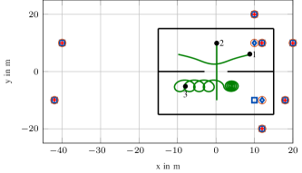
(a)

(b)

Figure 2: Considered scenario for performance evaluation. The start of each trajectory is indicated by a black dot and the visibility is determined at the end of the trajectories. Note that not all VAs are shown.

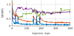
(a)

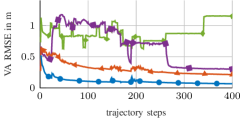
(b)

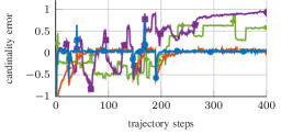
(c)

(d)

Figure 3: Comparison of different experimental settings. (a) shows the MOSPA, (b) the RMSE of the position errors of estimated VAs that were correctly associated to a true VA and (c) shows the cardinaltiy error. The results are averaged over all simulation runs and estimated VAs. The legend description can be found in Table I.

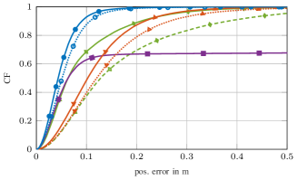
(a)

(b)

Figure 4: Cumulative frequency of MT position errors for different settings.The legend description can be found in Table I.

VI Numerical Results

We consider an indoor scenario shown in Fig. 2. The scenario consists of two BSs and five reflective surfaces, i.e., $5$ VAs per BS. Three MTs move along tracks which are observed for $400$ time instances $n$ with observation period $\Delta T=1\,$s. Measurements are generated according to the proposed system model in Section IV. The signal-to-noise-ratio (SNR) is set to $40\,\mathrm{dB}$ at an LOS distance of $1\,$m. The amplitudes of the main-components (LOS component and the MPCs) are calculated using a free-space path loss model and an additional attenuation of $3\,\mathrm{dB}$ for each reflection at a surface. We define $p_{\text{d}}=0.98$. In addition false positive measurements are generated according to the model in Section IV with a mean number of $\mu_{\text{fp}}=5$. For the calculation of the measurement variances, we assume a $3\text{-}\mathrm{dB}$ system bandwidth of $B=500\,\mathrm{MHz}$ with some known transmit signal spectrum at a carrier frequency of $f_{\mathrm{c}}=6\,\mathrm{GHz}$. The arrays employed at MTs and PAs are of identical geometry with $H=H^{(j)}=4$ antenna elements in (known) uniform rectangular array (URA)-configuration spaced at $\lambda/2$, where $\lambda=c/f_{\mathrm{c}}$ is the carrier wavelength. We use $10^{4}$ particles. The particles for the initial MT states are drawn from a 5-D uniform distribution with center $\bm{x}_{i,0}=[\bm{p}_{i,0}^{\text{T}}\;0\;\,0;\,o_{i,0}]^{\text{T}}$, where $\bm{p}_{i,0}$ is the starting position of the actual MT track, and the support of each position component about the respective center is given by $[-0.1\,\mathrm{m},0.1\,\mathrm{m}]$ and for each velocity component by $[-0.01\,\mathrm{m/s},0.01\,\mathrm{m/s}]$. If an IMU is used, the orientation state is represented by quaternions and are initialized using a 4-D Gaussian distribution with the center being the initial IMU measurements transformed to the quaternion representation and a standard deviation of $10^{\circ}$ [33]. At time $n=0$, the number of VAs is $0$, i.e., no prior map information is available. The prior distribution for new PVA states $f_{\text{n}}\big{(}\overline{\bm{x}}^{(j)}_{m,n}|\bm{x}_{n}\big{)}$ is uniform on the square region given by $[-\text{45 m},\text{45 m}]\times[-\text{45 m},\text{45 m}]$ around the center of the floor plan shown in Fig. 2 and the mean number of new PVAs at time $n$ is $\mu_{\text{n}}=0.01$. The probability of survival is $p_{\mathrm{s}}=0.999$. The confirmation threshold as well as the pruning threshold are given as $p_{\mathrm{cf}}=0.5$ and $p_{\mathrm{pr}}=10^{-3}$, respectively. For the sake of numerical stability, we introduce a small amount of regularization noise to the VA state $\bm{p}_{k,\mathrm{va}}$ at each time step $n$, i.e., $\underline{\bm{p}}^{(j)}_{k,\mathrm{va}}=\bm{p}^{(j)}_{k,\mathrm{va}}+\bm{\omega}_{k}$, where $\bm{\omega}_{k}$ is independent and identically distributed (iid) across $k$, zero-mean, and Gaussian with covariance matrix $\sigma_{a}^{2}\,\bm{I}_{2}$ and $\sigma_{a}=10^{-3}\,\text{m}$. The MTs state transition for position and velocity is modeled by a constant-velocity and stochastic-acceleration model. In the case of IMU measurements, the stochastic acceleration term is replaced by the control term $\bm{c}_{i,n-1}$[33, 37]. The state transition variances are set as $\sigma_{\text{w}}=10^{-3}\,\mathrm{m/s^{2}}$. The performance is measured in terms of the root mean squared error (RMSE) of the MT position as well as the optimal subpattern assignment (OSPA) error [38] of all VAs with cutoff parameter and order set to 1 m and 2, respectively. The mean (MOSPA) errors and RMSEs of each unknown variable are obtained by averaging over all simulation runs.

Experiment

For the investigation of the proposed method, we define different experiments as shown in Table I and perform $100$ simulation runs for each setting.

TABLE I: Boolean table for experimental settings

	$E_{1}$	$E_{2}$	$E_{3}$	$E_{4}$	$E_{5}$	$E_{6}$	$E_{7}$
MIMO	0	1	1	0	0	1	1
Coop	0	0	1	0	1	0	1
IMU	1	1	0	1	1	1	1
PVA Fusion	0	0	1	1	1	1	1

The results are summarized in Fig. 3 and Fig. 4. In Fig. 3, we present the MOSPA as well as the RMSE of the estimated VAs and the cardinality error for four settings. The best result can be achieved using the proposed algorithm with PVA data fusion, cooperation, IMU measurements and MIMO system ($E_{7}$). A comparable result can be reached using the same settings but SIMO instead of MIMO ($E_{5}$). Using the proposed algorithm but without IMU measurements leads to a significant performance loss. This can be explained by the complex trajectory of MT $i=3$, since it can not be well described by the constant velocity motion model without an additional control term ($E_{3}$). Using the state-of-the-art MP-SLAM with IMU measurements and the MIMO system but without PVA data fusion and cooperation ($E_{2}$) leads to the overall worst result, highlighting the significance of PVA fusion for robust and accurate mapping. Fig. 4 shows the cumulative frequency (CF) of all MTs and all time steps for different experiments. The benefit of PVA data fusion and cooperative localization vs non-cooperative localization is clearly demonstrated for MIMO and SIMO systems ($E_{6}$ vs $E_{7}$ and $E_{4}$ vs $E_{5}$). As a comparison to the proposed method, we show the impact of not using PVA fusion on the MTs positioning error for SIMO and MIMO ($E_{1}$ and $E_{2}$). Interestingly the proposed method without IMU measurements ($E_{3}$) has the most outliers. This can be explained in since one of the MTs has a very complex trajectory, which often diverges due to missing navigation input. These errors are propagated through the cooperation and the PVA data fusion resulting in an overall diminished performance.

VII Conclusions

In this work, we present a novel approach for MP-SLAM that performs data fusion over multiple observations of VAs by multiple MTs for robust and accurate mapping. This exchange of information for MTs also allows for cooperative localization in addition to multipath-based localization. We demonstrate, based on numerical simulations, the advantage of cooperative map fusion over state-of-the-art MP-SLAM without map-fusion. In addition, we present the advantage of using additional IMU measurements to deal with complex trajectories.

Appendix A Signal Model

Each BS transmits at a center frequency $f_{\text{c}}$ an RF signal $s^{(j)}_{\text{bs}}(t)$ with bandwidth $B$ and the MTs act as receivers. The RF signal arrives at the receiver via the LOS path as well as via MPCs originating from the reflections at surrounding objects. We assume time synchronization between all BSs and the MTs. However, our algorithm can be straightforwardly extended to an unsynchronized system according to [6, 2, 39]. We assume the BSs to use orthogonal codes, i.e., there is no mutual interference between individual BSs. Note that the proposed algorithm can be easily reformulated for the case where the MTs transmits RF signals and the BSs act as receivers. The received signals at the $I$ MTs are synchronously sampled with sampling frequency given by the signal bandwidth $B$. In frequency domain, this results in $M=B/\Delta$ samples with frequency spacing $\Delta$. The discrete-frequency RF signal model between BS $j$ and MT $i^{\prime}$ is given by [16]

$${r_{\text{bs}}}_{n}^{(j,i^{\prime})}[\ell,h,h^{\prime}] =\sum_{l=1}^{{N_{\text{bs}}}_{n}^{(j,i^{\prime})}}\exp{\big{(}i2\pi\frac{f_{\mathrm{c}}}{c}d^{(j,h)}\cos\big{(}{\vartheta}^{(j,i^{\prime})}_{l,n}-\psi^{(j,h)}\big{)}\big{)}}$$

$$\times\exp{\big{(}i2\pi\frac{f_{\mathrm{c}}}{c}d^{(i^{\prime},h^{\prime})}\cos\big{(}{\theta}^{(j,i^{\prime})}_{l,n}-o_{i^{\prime},n}-\psi^{(i^{\prime},h^{\prime})}\big{)}\big{)}}$$

$$\times\bm{s}({\tau_{\text{bs}}}_{l,n}^{(j,i^{\prime})})[\ell]+\hskip 0.85358pt{w_{\text{bs}}}_{n}^{(j,i^{\prime})}[\ell,h,h^{\prime}]$$ (20)

where $\bm{s}(\tau)[\ell]={\alpha_{\text{bs}}}_{l,n}^{(j,i)}S^{(j)}_{\text{bs}}(\ell\Delta)\exp{\big{(}i2\pi\ell\Delta\tau\big{)}}$, ${{N_{\text{bs}}}_{n}^{(j,i)}}$ is the number of visible path (related to VAs), $S^{(j)}_{\text{bs}}(f)$ represents the signal spectrum (we assume here that $S^{(j)}_{\text{bs}}(f)=S_{\text{bs}}(f)$), $\ell=-(M-1)/2,\hskip 2.84526pt\ldots\hskip 2.84526pt,(M-1)/2$, $h$ represent the index for BS antennas, $h^{\prime}$ represents the index for MT antennas. Delay, AOA and AOD of the MPC are represented by ${\tau_{\text{bs}}}_{l,n}^{(j,i)}$, $\theta^{(j,i)}_{l,n}$and $\vartheta^{(j,i)}_{l,n}$ respectively (see Fig. 1). The associated complex amplitude $\alpha_{l,n}^{(j,i)}\in\mathbb{C}$ is given by ${\alpha_{\text{bs}}}_{l,n}^{(j,i)}={a_{\text{bs}}}^{(j,i)}_{l,n}\hskip 0.85358pt\text{e}^{-j2\pi f_{\text{c}}{\tau_{\text{bs}}}_{l,n}^{(j,i)}}\frac{c}{4\pi f_{\text{c}}{d_{\text{bs}}}_{l,n}^{(j,i)}}$ where ${a_{\text{bs}}}^{(j,i)}_{l,n}\in\mathbb{C}$ is a reflection coefficient originating from all interactions of the radio signal with the radio equipment and the associated flat surfaces. The last term ${w_{\text{bs}}}_{n}^{(j,i)}[\ell,h]$ aggregates samples of the measurement noise and of a dense multipath component (DMC) that incorporates the contributions from all other interactions, e.g. diffuse scattering and diffraction. It also includes low-power MPCs that cannot be resolved with the finite bandwidth [16]. The receive signal samples for BS-MT links are collected into the vector $\bm{r}^{(j,i)}_{n}\in\mathbb{C}^{MHH^{\prime}}$ as

$$\bm{r}^{(j,i)}_{\text{bs}_{n}}= \big{[}\bm{r}_{\text{bs}_{n}}^{(j,i)\hskip 0.85358pt\text{T}}[1,1]\hskip 2.84526pt\cdots\hskip 2.84526pt\bm{r}_{\text{bs}_{n}}^{(j,i)\hskip 0.85358pt\text{T}}[H,1]\hskip 2.84526pt\bm{r}_{\text{bs}_{n}}^{(j,i)\hskip 0.85358pt\text{T}}[1,2]\hskip 2.84526pt\cdots\hskip 2.84526pt$$

$$\bm{r}_{\text{bs}_{n}}^{(j,i)\hskip 0.85358pt\text{T}}[H,H^{\prime}]\big{]}^{\text{T}}$$ (21)

The discrete-frequency RF signal model exchanged between MTs is given as $\bm{r}^{(i,i^{\prime})}_{\text{mt}_{n}}$ and can be obtained similarly to (A) with the difference that the orientation of each MT has to be considered. The receive signal samples for MT-MT links are collected in the same manner as (A). We assume that the signal spectrum for MT-MT links is $S^{(i)}_{\text{mt}}(f)=S_{\text{bs}}(f)$.

Appendix B Data Association

B-A Base Stations

At each time $n$ and for each BS $j$, estimation of multiple PVA states is complicated by the data association uncertainty, i.e., it is unknown which measurement ${\bm{\mathsfbr{z}}_{\text{bs}}}^{(j,i)}_{n}$ originated from which PVA. Furthermore, it is not known if a measurement did not originate from a PVA (i.e., a false alarm described by $\mu_{\mathrm{fa}}$ and PDF $f_{\mathrm{fa}}({\bm{z}_{\text{bs}}}^{(j,i)}_{m,n})$), or if a PVA did not give rise to any measurement missed detection). Following [40, 26, 3], we assume that at any time $n$, each PVA can generate at most one measurement, and each measurement can be generated by at most one PVA. The associations between measurements and legacy PVAs are described by the PVA-oriented association vector $\underline{\bm{\mathsfbr{a}}}_{n}^{(j,i)}\triangleq[\underline{\mathsfbr{a}}_{1,n}^{(j,i)}\hskip 0.85358pt\cdots\hskip 0.85358pt\underline{\mathsfbr{a}}_{\mathsfbr{K}^{(j)}_{n-1},n}^{(j,i)}]^{\mathrm{T}}$ with entries $\underline{\mathsfbr{a}}_{k,n}^{(j,i)}\triangleq m\in{{\cal{M}}_{\text{bs}}}_{n}^{(j,i)}$ if legacy PVA $k$ generates measurement $m$ or $\underline{\mathsfbr{a}}_{k,n}^{(j,i)}\triangleq 0$ if legacy PVA $k$ does not generate any measurement. In line with [40, 26, 3], the associations can be equivalently described by a measurement-oriented association vector $\overline{\bm{\mathsfbr{a}}}_{n}^{(j,i)}\triangleq[\overline{\mathsfbr{a}}_{1,n}^{(j,i)}\hskip 0.85358pt\cdots\hskip 0.85358pt\overline{\mathsfbr{a}}_{{\mathsfbr{M}_{\text{bs}}}_{n}^{(j,i)},n}^{(j,i)}]^{\mathrm{T}}$ with entries ${\overline{\mathsfbr{a}}}^{(j,i)}_{m,n}\triangleq k\in{{\cal{K}}}_{n}^{(j,i)}$ if measurement $m$ is originated by legacy PVA $k$ or ${\overline{\mathsfbr{a}}}^{(j,i)}_{m,n}\triangleq 0$ if measurement $m$ is not generated by any legacy PVA $k$. The point target assumption is enforced by the exclusion function $\Psi(\underline{\bm{a}}_{n}^{(j,i)},\overline{\bm{a}}_{n}^{(j,i)})=\prod_{k=1}^{K_{n-1}^{(j)}}\prod_{m=1}^{{M_{\text{bs}}}_{n}^{(j,i)}}\psi(\underline{a}_{k,n}^{(j,i)},\overline{a}_{m,n}^{(j,i)})$ with $\psi(\underline{a}_{k,n}^{(j)},\overline{a}_{m,n}^{(j)})=0$, if $\underline{a}_{k,n}^{(j)}=m$ and $\overline{a}_{m,n}^{(j)}\neq k$ or $\overline{a}_{m,n}^{(j)}=k$ and $\underline{a}_{k,n}^{(j)}\neq m$, otherwise it equals $1$. The “redundant formulation” of using $\underline{\bm{\mathsfbr{a}}}_{n}^{(j,i)}$ together with $\overline{\bm{\mathsfbr{a}}}_{n}^{(j,i)}$ is the key to making the algorithm scalable for large numbers of PVAs and measurements [26]. The vectors containing all association variables up to time $n$ are given for legacy PVAs by $\underline{\bm{\mathsfbr{a}}}_{1:n}\triangleq[\underline{\bm{\mathsfbr{a}}}_{1}^{\mathrm{T}}\,...\,\underline{\bm{\mathsfbr{a}}}_{n}^{\mathrm{T}}]^{\mathrm{T}}$ with $\underline{\bm{\mathsfbr{a}}}_{n}\triangleq[\underline{\bm{\mathsfbr{a}}}_{n}^{(1)\hskip 0.85358pt\mathrm{T}}\,...\,\underline{\bm{\mathsfbr{a}}}_{n}^{(J)\mathrm{T}}]^{\mathrm{T}}$ and $\underline{\bm{\mathsfbr{a}}}^{(j)}_{n}\triangleq[\underline{\bm{\mathsfbr{a}}}_{n}^{(j,1)\hskip 0.85358pt\mathrm{T}}\,...\,\underline{\bm{\mathsfbr{a}}}_{n}^{(j,I)\mathrm{T}}]^{\mathrm{T}}$ and for new PVAs by $\overline{\bm{\mathsfbr{a}}}_{1:n}\triangleq[\overline{\bm{\mathsfbr{a}}}_{1}^{\mathrm{T}}\,...\,\overline{\bm{\mathsfbr{a}}}_{n}^{\mathrm{T}}]^{\mathrm{T}}$ with $\overline{\bm{\mathsfbr{a}}}_{n}\triangleq[\overline{\bm{\mathsfbr{a}}}_{n}^{(1)\hskip 0.85358pt\mathrm{T}}\,...\,\overline{\bm{\mathsfbr{a}}}_{n}^{(J)\mathrm{T}}]^{\mathrm{T}}$ and $\overline{\bm{\mathsfbr{a}}}_{n}^{(j)}\triangleq[\overline{\bm{\mathsfbr{a}}}_{n}^{(j,1)\hskip 0.85358pt\mathrm{T}}\,...\,\overline{\bm{\mathsfbr{a}}}_{n}^{(j,I)\mathrm{T}}]^{\mathrm{T}}$.

B-B Cooperation

At each time $n$ and for each MT-pair $(i,i^{\prime})$ with $i\neq i^{\prime}$, the measurements, i.e., the components of ${\bm{\mathsfbr{z}}_{\text{co}}}^{(i,i^{\prime})}_{m,n}\in{\mathcal{M}_{\text{co}}}^{(i,i^{\prime})}_{n}$ are subject to the same data association uncertainty as mentioned before regarding LOS identification and association. The association variable $\mathsfbr{b}^{(i,i^{\prime})}_{n}$ for $i\neq i^{\prime}$ is given by $\mathsfbr{b}^{(i,i^{\prime})}_{n}=m\in{\mathcal{M}_{\text{co}}}^{(i,i^{\prime})}_{n}$ if LOS path is generated by measurement $m$ or $\mathsfbr{b}^{(i,i^{\prime})}_{n}=0$ otherwise. We also define $\bm{\mathsfbr{b}}_{1:n}\triangleq[\bm{\mathsfbr{b}}_{1}^{\mathrm{T}}\,...\,\bm{\mathsfbr{b}}_{n}^{\mathrm{T}}]^{\mathrm{T}}$ with $\bm{\mathsfbr{b}}_{n}\triangleq[\mathsfbr{b}^{(1,2)\hskip 0.85358pt\mathrm{T}}_{n}\hskip 2.84526pt\mathsfbr{b}^{(1,3)\hskip 0.85358pt\mathrm{T}}_{n}\,\cdots\,\mathsfbr{b}^{(I,I)\hskip 0.85358pt\mathrm{T}}_{n}]^{\mathrm{T}}$.

References

• [1] K. Witrisal, P. Meissner, E. Leitinger, Y. Shen, C. Gustafson, F. Tufvesson, K. Haneda, D. Dardari, A. F. Molisch, A. Conti, and M. Z. Win, “High-accuracy localization for assisted living: 5G systems will turn multipath channels from foe to friend,” IEEE Signal Process. Mag., vol. 33, no. 2, pp. 59–70, Mar. 2016.
• [2] C. Gentner, T. Jost, W. Wang, S. Zhang, A. Dammann, and U. C. Fiebig, “Multipath assisted positioning with simultaneous localization and mapping,” IEEE Trans. Wireless Commun., vol. 15, no. 9, pp. 6104–6117, Sept. 2016.
• [3] E. Leitinger, F. Meyer, F. Hlawatsch, K. Witrisal, F. Tufvesson, and M. Z. Win, “A belief propagation algorithm for multipath-based SLAM,” IEEE Trans. Wireless Commun., vol. 18, no. 12, pp. 5613–5629, Dec. 2019.
• [4] E. Leitinger, S. Grebien, and K. Witrisal, “Multipath-based SLAM exploiting AoA and amplitude information,” in Proc. IEEE ICCW-19, Shanghai, China, May 2019, pp. 1–7.
• [5] R. Mendrzik, F. Meyer, G. Bauch, and M. Z. Win, “Enabling situational awareness in millimeter wave massive MIMO systems,” IEEE J. Sel. Topics Signal Process., vol. 13, no. 5, pp. 1196–1211, Sep. 2019.
• [6] E. Leitinger, P. Meissner, C. Rudisser, G. Dumphart, and K. Witrisal, “Evaluation of position-related information in multipath components for indoor positioning,” IEEE J. Sel. Areas Commun., vol. 33, no. 11, pp. 2313–2328, Nov. 2015.
• [7] T. Wilding, S. Grebien, E. Leitinger, U. Mühlmann, and K. Witrisal, “Single-anchor, multipath-assisted indoor positioning with aliased antenna arrays,” in Proc. Asilomar-18, Pacifc Grove, CA, USA, Oct. 2018.
• [8] A. Shahmansoori, G. E. Garcia, G. Destino, G. Seco-Granados, and H. Wymeersch, “Position and orientation estimation through millimeter-wave MIMO in 5G systems,” IEEE Trans. Wireless Commun., vol. 17, no. 3, pp. 1822–1835, Mar. 2018.
• [9] R. Mendrzik, H. Wymeersch, G. Bauch, and Z. Abu-Shaban, “Harnessing NLOS components for position and orientation estimation in 5G millimeter wave MIMO,” IEEE Trans. Wireless Commun., vol. 18, no. 1, pp. 93–107, Jan. 2019.
• [10] H. Durrant-Whyte and T. Bailey, “Simultaneous localization and mapping: Part I,” IEEE Robot. Autom. Mag., vol. 13, no. 2, pp. 99–110, Jun. 2006.
• [11] M. Montemerlo, S. Thrun, D. Koller, and B. Wegbreit, “FastSLAM: A factored solution to the simultaneous localization and mapping problem,” in Proc. AAAI-02, Edmonton, Canda, Jul. 2002, pp. 593–598.
• [12] H. Deusch, S. Reuter, and K. Dietmayer, “The labeled multi-Bernoulli SLAM filter,” IEEE Signal Process. Lett., vol. 22, no. 10, pp. 1561–1565, Oct. 2015.
• [13] X. Chu, Z. Lu, D. Gesbert, L. Wang, X. Wen, M. Wu, and M. Li, “Joint vehicular localization and reflective mapping based on team channel-SLAM,” IEEE Trans. Wireless Commun., pp. 1–1, Apr. 2022.
• [14] D. Shutin, W. Wang, and T. Jost, “Incremental sparse Bayesian learning for parameter estimation of superimposed signals,” in Proc. SAMPTA-2013, no. 1, Sept. 2013, pp. 6–9.
• [15] T. L. Hansen, B. H. Fleury, and B. D. Rao, “Superfast line spectral estimation,” IEEE Trans. Signal Process., vol. PP, no. 99, pp. 2511 – 2526, Feb. 2018.
• [16] S. Grebien, E. Leitinger, K. Witrisal, and B. H. Fleury, “Super-resolution estimation of UWB channels including the dense component — an SBL-inspired approach,” pp. 1–1, 2024.
• [17] X. Li, E. Leitinger, A. Venus, and F. Tufvesson, “Sequential detection and estimation of multipath channel parameters using belief propagation,” IEEE Trans. Wireless Commun., pp. 1–1, Apr. 2022.
• [18] L. Wielandner, A. Venus, T. Wilding, and E. Leitinger, “Multipath-based SLAM for non-ideal reflective surfaces exploiting multiple-measurement data association,” Journal of Advances in Information Fusion, vol. 18, no. 2, 2023. [Online]. Available: https://isif.org/issue/jaif-volume-18-issue-2
• [19] L. Wielandner, A. Venus, T. Wilding, K. Witrisal, and E. Leitinger, “MIMO multipath-based SLAM for non-ideal reflective surfaces,” 2024. [Online]. Available: http://arxiv.org/pdf/2404.15375
• [20] E. Leitinger, A. Venus, B. Teague, and F. Meyer, “Data fusion for multipath-based SLAM: Combining information from multiple propagation paths,” IEEE Trans. Signal Process., vol. 71, pp. 4011–4028, Sep. 2023.
• [21] P. Sharma, A.-A. Saucan, D. J. Bucci, and P. K. Varshney, “Decentralized gaussian filters for cooperative self-localization and multi-target tracking,” IEEE Trans. Signal Process., vol. 67, no. 22, pp. 5896–5911, 2019.
• [22] M. Brambilla, D. Gaglione, G. Soldi, R. Mendrzik, G. Ferri, K. D. LePage, M. Nicoli, P. Willett, P. Braca, and M. Z. Win, “Cooperative localization and multitarget tracking in agent networks with the sum-product algorithm,” IEEE Open Journal of Signal Processing, vol. 3, pp. 169–195, 2022.
• [23] H. Kim, K. Granström, L. Gao, G. Battistelli, S. Kim, and H. Wymeersch, “5G mmWave cooperative positioning and mapping using multi-model PHD filter and map fusion,” IEEE Trans. Wireless Commun., vol. 19, no. 6, pp. 3782–3795, Mar. 2020.
• [24] L. Wielandner, E. Leitinger, F. Meyer, and K. Witrisal, “Message passing-based 9-D cooperative localization and navigation with embedded particle flow,” IEEE Trans. Signal Inf. Process. Netw., vol. 9, pp. 95–109, 2023.
• [25] J. Borish, “Extension of the image model to arbitrary polyhedra,” JASA, vol. 75, no. 6, pp. 1827–1836, Mar. 1984.
• [26] F. Meyer, T. Kropfreiter, J. L. Williams, R. Lau, F. Hlawatsch, P. Braca, and M. Z. Win, “Message passing algorithms for scalable multitarget tracking,” Proc. IEEE, vol. 106, no. 2, pp. 221–259, Feb. 2018.
• [27] S. M. Kay, Fundamentals of Statistical Signal Processing: Estimation Theory.   Upper Saddle River, NJ, USA: Prentice Hall, 1993.
• [28] K. Witrisal, E. Leitinger, S. Hinteregger, and P. Meissner, “Bandwidth scaling and diversity gain for ranging and positioning in dense multipath channels,” IEEE Wireless Commun. Lett., vol. 5, no. 4, pp. 396–399, May 2016.
• [29] A. Fascista, B. J. B. Deutschmann, M. F. Keskin, T. Wilding, A. Coluccia, K. Witrisal, E. Leitinger, G. Seco-Granados, and H. Wymeersch, “Uplink joint positioning and synchronization in cell-free deployments with radio stripes,” in Proc. IEEE ICC 2023, Rome, Italy, May 2023.
• [30] Y. Bar-Shalom, X. R. Li, and T. Kirubarajan, Estimation with Applications to Tracking and Navigation: Algorithms and Software for Information Extraction.   Hoboken, NJ: John Wiley and Sons, July 2001.
• [31] S. M. Kay, Fundamentals of Statistical Signal Processing: Detection Theory.   Upper Saddle River, NJ, USA: Prentice Hall, 1998.
• [32] A. Venus, E. Leitinger, S. Tertinek, and K. Witrisal, “A graph-based algorithm for robust sequential localization exploiting multipath for obstructed-LOS-bias mitigation,” IEEE Trans. Wireless Commun., vol. 23, no. 2, pp. 1068–1084, June 2023.
• [33] S. Madgwick et al., “An efficient orientation filter for inertial and inertial/magnetic sensor arrays,” Report x-io and University of Bristol (UK), vol. 25, pp. 113–118, 2010.
• [34] F. Kschischang, B. Frey, and H.-A. Loeliger, “Factor graphs and the sum-product algorithm,” IEEE Trans. Inf. Theory, vol. 47, no. 2, pp. 498–519, Feb. 2001.
• [35] F. Meyer, O. Hlinka, H. Wymeersch, E. Riegler, and F. Hlawatsch, “Distributed localization and tracking of mobile networks including noncooperative objects,” IEEE Trans. Signal Inf. Process. Netw., vol. 2, no. 1, pp. 57–71, Mar. 2016.
• [36] F. Meyer, P. Braca, P. Willett, and F. Hlawatsch, “A scalable algorithm for tracking an unknown number of targets using multiple sensors,” IEEE Trans. Signal Process., vol. 65, no. 13, pp. 3478–3493, July 2017.
• [37] J. D. Hol, F. Dijkstra, H. Luinge, and T. B. Schon, “Tightly coupled uwb/imu pose estimation,” in 2009 IEEE International Conference on Ultra-Wideband, 2009, pp. 688–692.
• [38] D. Schuhmacher, B.-T. Vo, and B.-N. Vo, “A consistent metric for performance evaluation of multi-object filters,” IEEE Trans. Signal Process., vol. 56, no. 8, pp. 3447–3457, Aug. 2008.
• [39] B. Etzlinger, F. Meyer, F. Hlawatsch, A. Springer, and H. Wymeersch, “Cooperative simultaneous localization and synchronization in mobile agent networks,” IEEE Trans. Signal Process., vol. 65, no. 14, pp. 3587–3602, July 2017.
• [40] J. Williams and R. Lau, “Approximate evaluation of marginal association probabilities with belief propagation,” IEEE Trans. Aerosp. Electron. Syst., vol. 50, no. 4, pp. 2942–2959, Oct. 2014.