Exploring Weak measurements within the Einstein-Dirac Cosmological framework

Abstract

Our study applies the Two-State Formalism alongside weak measurements within a spatially homogeneous and isotropic cosmological framework, wherein Dirac spinors are intricately coupled to classical gravity. To elucidate this, we provide detailed formulations for computing the weak values of the energy-momentum tensors, the Z component of spin, and the characterization of pure states. Weak measurements appear to be a generalization and extension of the computation already made by Finster an Hainzl, [1], in A spatially homogeneous and isotropic Einstein-Dirac cosmology. Our analysis reveals that the acceleration of the Universe expansion can be understood as an outcome of postselection, underscoring the effectiveness of weak measurement as a discerning approach for gauging cosmic acceleration.

I INTRODUCTION

Measuring involves assigning numerical values to the attributes or characteristics of a phenomenon. The impact of the observer on measurement results is a complex consideration in scientific research. In quantum mechanics, the alteration of a quantum state after its measurement is well known, but its interpretation is not obvious. For example, the famous double-slit experiment demonstrates that particles like electrons can behave as particles and waves, and measurement prescribes their behavior [2, 3].

Weak measurements offer a procedure to measure the system state that minimizes its disturbance with minimal perturbation, achieved through a weak coupling between the measurement apparatus and the system’s state. Notably, these measurements enable the characterization of a particle’s trajectory in the double-slit experiment without disrupting the interference pattern, as demonstrated in previous studies [3, 4, 5, 6]. Unlike classical or ideal measurements, which result in the stochastic collapse of the system state into one of the eigenstates of the measured observable [7], weak measurements do not induce a collapse of the state vector. Instead, they introduce a small angular bias to the state vector, and the measurement device exhibits a superposition of multiple values rather than a clear eigenvalue [4]. Consequently, weak measurements unveil unconventional weak values, including complex numbers.

In literature, some authors have explored weak measurement and Two-state vectors formalism within the theoretical framework of cosmology and ontology. George Ellis and Rotman [8] proposed a paradigm that challenges conventional notions of time and reality, termed the Crystallizing Block Universe (CBU), an extension of the Emergent Block Universe (EBU). According to their perspective, past, present, and future coalesce, amalgamating space-time into a singular entity. The future is conceptualized as a superposition of myriad possibilities, while the past remains immutable. The transition between these temporal states predominantly unfolds in the present, albeit in a non-uniform manner. Within the CBU framework, certain discrete patches of quantum indeterminacy endure and are resolved later on. Furthermore, CBU models integrate the Two-time interpretation [9] of quantum mechanics. Nevertheless, this theoretical and ontological paradigm lies beyond the purview of our current study.

Davies [10] is the first to propose applying weak measurements theory combined with pre-and-post-selection to quantum cosmology and to explore the potential large-scale cosmological effects arising from this new sector of quantum mechanics. He illustrated the theory with a two-spacetime dimensional toy model of a scalar field with mass $m$ propagating in an expanding Universe with the scale factor $a(t)$ and metric $ds^{2}=dt^{2}-a(t)dx^{2}$. He resolved a debate regarding the coupling of pre- and postselected quantum fields to the gravity and proposed an experimental test for weak values in cosmology. He observed that in the literature, in equation $G_{\mu\nu}+\text{higher order terms in curvature }=\frac{\langle 0_{fin}|T_{\mu\nu}|0_{in}\rangle}{\langle 0_{fin}|0_{in}\rangle}$ originally derived by DeWitt, who adapted the Schwinger effective action theory of quantum electrodynamics to the gravitational case, the source term is nothing else than the weak values of the stress-energy-momentum tensor $T_{\mu\nu}$, [11]. This equation was widespread in 1970, [12], [13], [14].

After Davies’s paper [10], no research papers have been pursued in the direction of the theory of weak measurements in Cosmology until now. The subject seems to arouse interest. Charis Anastopoulos has just published on ar$\chi$iv a paper on Final States in Quantum Cosmology: Cosmic Acceleration as a Quantum Postselection Effect, [15] wherein he argues that there is no compelling physical reason to preclude a probability assignment with a final quantum state at the cosmological level and analyses its implications in quantum cosmology. One significant result is that cosmic acceleration emerges as a quantum postselection effect.

We aim to examine weak measurements of Dirac particles within the framework of time symmetry as applied to the Einstein-Dirac system in a homogeneous and isotropic space such as the Friedman-Lemaître-Robertson-Walker( FLRW) space. To the best of our knowledge, no prior research has explored this direction. Drawing upon insights from the paper of Finster and Hainzl, titled A Spatially Homogeneous and Isotropic Einstein-Dirac Cosmology [1], we endeavor to extend certain findings to the domain of weak measurements. Among the outcomes of our investigation are the computation of weak values, including those pertaining to energy-momentum, pure states, and the Z component of spin. Additionally, we demonstrate that the epochs of accelerated expansion in the Universe may be regarded as consequences of postselection. This corroborates earlier studies that have explored the potential of spinor fields to elucidate phenomena such as the inflationary period in the early universe and, subsequently, the concept of dark energy. Notably, Anastopoulos arrived at a similar conclusion, albeit without invoking a spinor field or dark energy, thus emphasizing alternative avenues for understanding the observed cosmological acceleration. Ribas reached the same conclusion without resorting to weak measurements or postselection techniques. References to relevant literature supporting these assertions include [16, 17, 18, 19, 20, 21].

In the time-symmetric formulation of quantum mechanics [22], a quantum system is not characterized by a single state vector but by Two-State vectors at a specific time. The preselected state is determined by measurements conducted on the system at times prior to $t_{0}$, while the postselected state by measurements at times $t>t_{0}$. The postselected state is conceptualized as a quantum state evolving backward in time. Weak measurements occur in the interval between these conventional measurements through a weak coupling between the measurement apparatus and the system [4].

Formally, if $\hat{A}$ is a Hermitian operator on the system $S$, $|\psi_{in}\rangle$ and $|\psi_{out}\rangle$ (or $|\psi_{fin}\rangle$) are the preselected and postselected state vectors in the Hilbert space of $S$, and $|\phi(x)\rangle$ is the state vector of the needle of the measurement device, $g(t)$ a coupling impulse such that $\int_{0}^{T}g(t)dt=1$, $T$ the coupling time and $\hat{P}_{d}$ the momentum conjugated operator to $\hat{Q}_{d}$ the position operator, then weakly measuring an ensemble of preselected vectors states $|\psi_{in}\rangle$ with $\hat{H}=g(t)\hat{A}\otimes\hat{P}_{d}$ the interaction Hamiltonian yields the following amplitude to get the postselected state vector: $\langle\psi_{fin}|e^{(-i\hat{H}T)}|\psi_{in}\rangle$. In detail, this is obtained as follows: let $\hat{P}=|\psi_{fin}\rangle\langle\psi_{fin}|\otimes\hat{I}$ be an operator which projects onto the postselected state $|\psi_{fin}\rangle$, and $|\psi_{w}\rangle=e^{(-i\hat{H}T)}|\psi_{in}\rangle\otimes|\phi(x)\rangle$ the entangled state of the system with the collapsed state of the measurement device [4],[23]. Then we get

$$\hat{P}|\psi_{w}\rangle =|\psi_{fin}\rangle\langle\psi_{fin}|e^{(-i\hat{H}T)}|\psi_{in}\rangle\otimes|\phi(x)\rangle$$

Assuming that $\hat{P}_{d}$ is distributed around 0 with low variance, its conjugate variable $\hat{Q}_{d}$ will have high variance, and the measurement will be weak. Hence, we shall get:

$$|\psi_{fin}\rangle\langle\psi_{fin}|(1-i\hat{A}\otimes\hat{P}_{d}\cdot T)|\psi_{in}\rangle\otimes|\phi(x)\rangle$$

$$=|\psi_{fin}\rangle\otimes\langle\psi_{fin}|\psi_{in}\rangle e^{-i\left(\langle\hat{A}\rangle_{w}\hat{P}_{d}T\right)}$$

where $\langle\hat{A}\rangle_{w}=\frac{\langle\psi_{fin}|\hat{A}|\psi_{in}\rangle}{\langle\psi_{fin}|\psi_{in}\rangle}$ is the so-called weak measurement of the observable $\hat{A}$. The probabilities to get this result is $|\langle\psi_{fin}|\psi_{in}\rangle|^{2}$.

Weak values are weak measurement results and must be understood as statistical averages. They are also members of a decomposition of eigenvalues weighted by the relative probabilities of finding the out states among the ensemble of states vectors identically prepared in $|\psi_{in}\rangle$. Weak measurement should then be understood as a conditional probability where one of the events undergoes a perturbation. Dressel [24] clarifies this probabilistic understanding of weak values. He shows that weak values characterize the relative correction to a detection probability $|\langle\psi_{fin}|\psi_{in}\rangle|^{2}$ due to a small intermediate perturbation $\hat{U}(\epsilon)$ that results in a modified detection probability $|\langle\psi_{fin}|\hat{U}(\epsilon)\psi_{in}\rangle|^{2}$. Alternatively, in a simple way, he defines weak values as complex numbers that one can assign to the powers of a quantum observable operator $\hat{A}$ using two states: an initial state $|\psi_{in}\rangle$ and a final state $|\psi_{fin}\rangle$. Weak values might lie outside the spectrum of eigenvalues and can be complex numbers. One interesting phenomenon is the amplification obtained when the preselected state and the postselected one are almost orthogonal [4, 10].

In cosmology [10], all observations and measurements are considered weak in the quantum sense due to the nature of the processes involved. For instance, when observing the redshift of a galaxy, the measurement is conducted by observing the light emitted from a large number of photons originating from numerous sources within the galaxy. While the emission of a single photon from an atom may not be considered weak from the atom’s perspective, the use of a large ensemble of photons to measure a property of the entire galaxy constitutes a weak measurement in the quantum sense. This is because the quantum back-reaction of the photons on the relevant physical variable of the entire galaxy, such as its momentum, is negligible. Therefore, the large-scale nature of cosmological observations and measurements, involving statistical averages over a large ensemble of photons, results in weak values in the quantum sense.

In the laboratory, the Two-State vectors require human interventions. In quantum cosmology, there are many proposals, as noticed by Davies: Hartle and Hawking came up with the no-boundary wave function, which is the state of the Universe before the Planck epoch [25]. In a semi-classical approach, in the framework of the theory of quantum fields, the initial state is taken to be a vacuum state. As for the final state, this can be anything. In weak measurement, one will ensure that the final state is not orthogonal to the in-state.

For the Einstein-Dirac in FLRW context, the preselected state will be the spinor solution of the Einstein-Dirac equation in the limit of the massless Universe, that is, the radiation Universe, whereas the final state will be the spinor solution of the Einstein-Dirac equation for the dust Universe. The implementation of weak measurement in this specific context is intended to acquire geometrical information about the Universe. The subsequent computational analysis is made feasible by the association between weak measurement and the Berry phase [7]. This has never been explored before, as far as we know.

Regarding the Einstein-Dirac system, it investigates the interaction between particles with a spin of $1/2$ and the gravitational field. The Einstein field equations essentially relate the geometry of spacetime to the distribution of matter and energy within that spacetime. In simpler terms, they describe how matter and energy, represented here by the stress tensor applied on spinors, influence the curvature of spacetime and how the curvature of spacetime influences the motion of matter and energy. Finster [1] investigated the nonlinear coupling of gravity to matter in a time-dependent, spherically symmetric Einstein-Dirac system. He showed that quantum oscillations of the Dirac wave functions can prevent the formation of a big bang or big crunch singularity.

Weak measurements present numerous advantages, foremost among them being the capability to detect exceedingly subtle effects while minimizing disturbance to the system state. Onur Hosten and Paul Kwiat [26] exemplified the utility of weak measurement techniques in amplifying the spin Hall effect, Meng-Jun Hu [27] discussed in his paper the proposal for Weak Measurements Amplification based Laser Interferometer Gravitational-wave Observatory (WMA-LIGO) to detect gravitational waves using weak measurements to amplify ultra-small phase signals, while Dixon et al. [28] applied these methods to enhance the detection of minute transverse deflections in an optical beam. This facet of weak measurements proves highly advantageous in cosmology, enabling the amplification and measurement of wave functions originating in the remote past, close to singularities.

This paper is organized as follows: After the introduction, we give a summary of the Einstein-Dirac system and then find the spinor solutions for the radiation Universe and the dust one. In section III, we give the results of our main computations on weak measurements on the Einstein-Dirac solutions.In section IV, we give a conclusion. The appendices provide some details of our computations.

II The Einstein-Dirac Solution in Friedmann-Lemaître-Robertson-Walker Space

In this section, we provide an overview of the Einstein-Dirac solution within the Friedmann-Lemaître-Robertson-Walker (FLRW) space framework. For a more comprehensive treatment, readers are encouraged to refer to [1] and [29].

The Einstein-Dirac (ED) equations are given by

$$R^{i}_{j}-\frac{1}{2}R\delta^{i}_{j}=8\pi\kappa T^{i}_{j},\quad(\mathcal{D}-m)\Psi=0,$$ (1)

where $\kappa$ represents the gravitational constant, $T^{i}_{j}$ the energy-momentum tensor of the Dirac particles, $\mathcal{D}$ the Dirac operator, $m$ the mass of the Dirac particles, and $\Psi$ the Dirac wave function.

Our Einstein-Dirac equations are formulated within the FLRW space, a spacetime manifold with a (1,3) signature. This simple cosmological model is characterized by a metric described by the homogeneous and isotropic line element

$$ds^{2}=dt^{2}-R^{2}(t)\left(\frac{dr^{2}}{1-kr^{2}}+r^{2}d\Omega^{2}\right),$$ (2)

where $t\in\mathbb{R}$ represents time, $(\theta,\phi)\in(0,\pi)\times[0,2\pi)$ are angular coordinates, $r$ is the radial coordinate, $R(t)$ the scale function, $d\Omega^{2}$ the line element on $S^{2}$, and $k$ can take values of -1, 0, or 1, corresponding to open, flat, and closed universes, respectively. We adopt ”Planck units” where $c=\hbar=G=1$.

In this article, we specifically consider the case of a closed universe with $k=1$, although similar computations can be extended to other cases. In this scenario, the line element simplifies to

$$ds^{2}=dt^{2}-R^{2}(t)\left(\frac{dr^{2}}{1-r^{2}}+r^{2}d\Omega^{2}\right).$$ (3)

In this case, the coordinate $r$ will vary in the interval $(0,1)$. After conducting detailed calculations, outlined in the appendices of [1] and [29], the Dirac operator takes the following form

$$\left[i\gamma\left(\partial_{t}+\frac{3}{2}\frac{\dot{R}}{R}\right)-R(t)m+\begin{pmatrix}0&\mathcal{D}_{\mathcal{H}}\\ -\mathcal{D}_{\mathcal{H}}&0\end{pmatrix}\right]\Psi=0,$$ (4)

where $\mathcal{D}_{\mathcal{H}}$ represents the purely spatial operator on $S^{3}$, given by

$$\mathcal{D}_{\mathcal{H}}=i\sigma^{r}\left(\partial_{r}+\frac{f-1}{rf}\right)+i\sigma^{\theta}\partial_{\theta}+\sigma^{\phi}\partial_{\phi},$$ (5)

where $\sigma^{r},\sigma^{\theta}\text{and}\sigma^{\phi}$ are linear combinations of the Pauli matrixes defined as follows

$$\left\{\begin{array}[]{lll}\sigma^{r}:=f(r)\left(\cos{\theta}\sigma^{3}+\sin{\theta}\cos{\phi}\sigma^{1}+\sin{\theta}\sin{\phi}\sigma^{2}\right)\\ \sigma^{\theta}:=\frac{1}{r}\left(-\sin{\theta}\sigma^{3}+\cos{\theta}\cos{\phi}\sigma^{1}+\cos{\theta}\sin{\phi}\sigma^{2}\right)\\ \sigma^{\phi}:=\frac{1}{r\sin{\theta}}\left(-\sin{\phi}\sigma^{1}+\cos{\phi}\sigma^{2}\right).\end{array}\right.$$ (9)

and the function

$$\begin{array}[]{lll}f(r)&=&\sqrt{1-r^{2}},\hskip 28.45274ptr\in(0,1)\\ \end{array}$$ (11)

This spatial operator $\mathcal{D}_{\mathcal{H}}$ has a purely discrete spectrum

$$\sigma(\mathcal{D}_{\mathcal{H}})=\left\{\pm\frac{3}{2},\pm\frac{5}{2},\pm\frac{7}{2},\ldots\right\},$$ (12)

and the dimension of the corresponding eigenspace is given as:

$$\text{dim}\;\text{ker}\left(\mathcal{D}_{\mathcal{H}}-\lambda\right)=\lambda^{2}-\frac{1}{4}.$$ (13)

An orthonormal eigenvector basis in terms of spherical harmonics and Jacobi polynomials is provided in the appendix of [29] and is denoted by $\psi^{\pm}_{njk}$, where $n\in\mathbb{N}_{0}$, $j\in\mathbb{N}_{0}+\frac{1}{2}$, and $k\in\{-j,-j+1,\ldots,j\}$.

The spatial differential operator on the eigenvector can be represented as follows

$$\mathcal{D}_{\mathcal{H}}\psi^{\pm}_{njk}=\lambda\psi^{\pm}_{njk},\quad\text{where}\quad\lambda=\pm(n+j+1).$$ (14)

We represent the normalized eigenfunction of $\mathcal{D}_{\mathcal{H}}$ related to the eigenvalue $\lambda$ by $\psi_{\lambda}\in L^{2}(S^{3})^{2}$.

To further analyze the system, we employ a separation ansatz for

$$\Psi=\frac{1}{R(t)^{\frac{3}{2}}}\begin{pmatrix}\alpha(t)\psi_{\lambda}(r,\theta,\phi)\\ \beta(t)\psi_{\lambda}(r,\theta,\phi)\end{pmatrix}.$$ (15)

This ansatz enables the derivation of a coupled system of ordinary differential equations (ODEs) for the complex-valued functions $\alpha(t)$ and $\beta(t)$:

$$i\frac{d}{dt}\begin{pmatrix}\alpha(t)\\ \beta(t)\end{pmatrix}=\begin{pmatrix}m&-\frac{\lambda}{R(t)}\\ -\frac{\lambda}{R(t)}&-m\end{pmatrix}\begin{pmatrix}\alpha(t)\\ \beta(t)\end{pmatrix}.$$ (16)

The spinors are normalized according to:

$$|\alpha|^{2}+|\beta|^{2}=\lambda^{2}-\frac{1}{4}.$$ (17)

These spinors enter the Einstein equation via the energy-momentum tensor of the wave function, ensuring a coupling with the Dirac equation. The non-vanishing components of the energy-momentum tensor are computed in Appendix B of [1] and are given by

$$T^{0}_{0} =R^{-3}\left[m\left(|\alpha|^{2}-|\beta|^{2}\right)-\frac{2\lambda}{R}\text{Re}\left(\alpha\bar{\beta}\right)\right],$$ (18)

$$T^{r}_{r} =T^{\theta}_{\theta}=T^{\phi}_{\phi}=R^{-3}\frac{2\lambda}{3R}\text{Re}\left(\alpha\bar{\beta}\right).$$ (19)

A short calculation for the Einstein tensor $G^{j}_{k}$, given in [1], yields

$$G_{0}^{0} =3\left(\frac{\dot{R}^{2}+1}{R^{2}}\right),$$ (20)

$$G_{r}^{r} =G_{\theta}^{\theta}=G_{\phi}^{\phi}=2\frac{\ddot{R}}{R}+\frac{\dot{R}^{2}+1}{R^{2}}.$$ (21)

Knowing that :

$$G^{i}_{j}=8\pi\kappa T^{i}_{j},\quad\text{where}\quad G^{i}_{j}=R^{i}_{j}-\frac{1}{2}R\delta^{i}_{j},$$

we set $\kappa=\frac{3}{8\pi}$ for a convenient computation as in [1]. This yields the following expression, the Einstein equation

$$\dot{R}^{2}+1=R^{2}T^{0}_{0},$$ (22)

which in terms of two level system is given as

$$\dot{R}^{2}+1=\frac{m}{R}\left(|\alpha|^{2}-|\beta|^{2}\right)-\frac{2\lambda}{R^{2}}\text{Re}\left(\alpha\bar{\beta}\right).$$ (23)

We derive also the acceleration of the Universe represented here by the second derivative with respect to time of the scale function given firstly in terms of the energy-momentum tensors as

$$\ddot{R}=\frac{R}{2}\left(3T^{j}_{j}-T^{0}_{0}\right).$$ (24)

Then in terms of spinors we shall have

$$\ddot{R}=-\frac{m}{2R^{2}}\left(|\alpha|^{2}-|\beta|^{2}\right)+\frac{2\lambda}{R^{3}}\text{Re}\left(\alpha\bar{\beta}\right).$$ (25)

One sees immediately that the acceleration of the Universe is caused by the spinor field, and this is consistent along the lines of [16, 17, 18, 19, 20, 21]. We will later on show some behaviours of the acceleration of the scale function.

At this stage, we are left with two differential equations, equations (16) and (23), in which the spinor $\begin{pmatrix}\alpha\\ \beta\end{pmatrix}$ is considered as a two-level quantum state.

As suggested by Finster and Hainzl in [1], the Einstein-Dirac equation can be rewritten in terms of a Bloch vector $\vec{v}$, where

$$\vec{v} =\begin{pmatrix}\langle\xi|\sigma^{1}|\xi\rangle\\ \langle\xi|\sigma^{2}|\xi\rangle\\ \langle\xi|\sigma^{3}|\xi\rangle\end{pmatrix},$$ (26)

$$\vec{b} =2\frac{\lambda}{R}\vec{e}_{1}-2m\vec{e}_{3}.$$ (27)

Here, $\xi$ represents the spinor $\begin{pmatrix}\alpha\\ \beta\end{pmatrix}$, $\sigma^{i}$ are the Pauli matrices, and $\vec{e}_{i}$ are the standard basis vectors in $\mathbb{R}^{3}$ ($i\in\{1,2,3\}$).

The Einstein-Dirac equations can then be expressed as

$$\dot{\vec{v}}=\vec{b}\wedge\vec{v},\quad\dot{R}^{2}+1=-\frac{1}{2R}\vec{b}\cdot\vec{v}.$$ (28)

Here, ‘$\wedge$’ and ‘$\cdot$’ denote the cross and scalar product in Euclidean space $\mathbb{R}^{3}$, respectively. We rewrite also the scale acceleration in terms of the Bloch vector components as

$$\ddot{R}=-\frac{m}{2R^{2}}v^{3}+\frac{\lambda}{R^{3}}v^{1}.$$ (29)

To simplify the analysis, a rotation“U” around the $\vec{e}_{2}$-axis is applied to $\vec{b}$, making $\vec{b}$ parallel to $\vec{e}_{1}$. This results in a transformed vector $\vec{w}$

$$\vec{w}=U\vec{v}=\begin{pmatrix}w^{1}\\ w^{2}\\ w^{3}\end{pmatrix}$$ (30)

where the components of $\vec{w}$ are given by

$$w^{1} =\frac{1}{\sqrt{\lambda^{2}+m^{2}R^{2}}}\left(2\lambda\text{Re}\left(\alpha\bar{\beta}\right)-mR\left(|\alpha|^{2}-|\beta|^{2}\right)\right),$$ (31)

$$w^{2} =2\text{Im}\left(\alpha\bar{\beta}\right),$$ (32)

$$w^{3} =\frac{1}{\sqrt{\lambda^{2}+m^{2}R^{2}}}\left(2m\text{Re}\left(\alpha\bar{\beta}\right)+\lambda\left(|\alpha|^{2}-|\beta|^{2}\right)\right).$$ (33)

At this stage, the Einstein-Dirac equations reduce to a system of ODEs involving the scale function $R(t)$ and the complex functions $\alpha(t)$ and $\beta(t)$

$$\dot{\vec{w}}=\vec{d}\wedge\vec{w},\quad\dot{R}^{2}+1=-\frac{1}{R^{2}}\sqrt{\lambda^{2}+m^{2}R^{2}}w^{1},$$ (34)

where $\vec{d}$ is defined as

$$\vec{d}:=\frac{2}{R}\sqrt{\lambda^{2}+m^{2}R^{2}}\vec{e}_{1}-\frac{\lambda mR}{\lambda^{2}+m^{2}R^{2}}\frac{\dot{R}}{R}\vec{e}_{2}.$$ (35)

The length of the Bloch vector is constant, and the normalization convention is

$$|\vec{w}|=\lambda^{2}-\frac{1}{4}=N.$$ (36)

Within weak measurement and the Two Vectors State Formalism this research primarily explores solutions to the Einstein-Dirac equation under specific conditions. These conditions involve both the mass parameter ($m$) and the coupling constant ($\lambda$) approaching zero. In this regime, we distinguish between preselected states and postselected states, the solutions of (34) for respectively $m=0$ and $\lambda=0$.

In the case where $m=0$, the Einstein-Dirac equation simplifies to the well-known FLRW equation, describing the Universe’s behaviour in the radiation-dominated phase. Conversely, in the second scenario, where $\lambda=0$, corresponds to a dust-dominated Universe. Notably, for sufficiently large values of the scale factor $R$, the Universe exhibits classical behaviour similar to the dust-dominated case.

The above assumption could be seen easily from the complete and classical Friedmann general equation with $k=1,0,-1$ corresponding to closed, flat and opened universe respectively

$$\dot{R}^{2}+k=-\left(\frac{\rho_{m}}{R}+\frac{\rho_{r}}{R^{2}}-\Lambda R^{2}\right),$$ (37)

where $\rho_{m}$ is the density of matter, $\rho_{r}$ is the density of radiation and $\Lambda$ is the vacuum energy. Just after the Big Bang, the Universe was too small. For $R\ll 1$, whatever the terms in the right side of the expression (37), the radiative one would dominate in the evolution of the Universe. The expression becomes

$$\dot{R}^{2}+k=-\left(\frac{\rho_{r}}{R^{2}}\right).$$ (38)

While, ignoring the vacuum energy, if $R\gg 1$, the mass term would dominate and the expression (37) becomes

$$\dot{R}^{2}+k=-\left(\frac{\rho_{m}}{R}\right),$$ (39)

This equation describes a dust-dominated Universe.

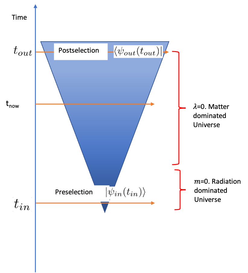
Figure 1: Preselection and Postselection à $t_{in}$ and $t_{out}$

It is essential to note that the radiation-dominated Universe pertains to a brief period near the initial singularity. In contrast, the dust-dominated universe extends over a much longer timeframe, including the present day.

II.1 $\mid\Psi_{in}\rangle$: Solution of the Einstein-Dirac equation for $m=0$.

When $m=0$, the ODEs in (34) becomes

$$\left\{\begin{array}[]{lll}\dot{w}^{1}&=&0\\ \dot{w}^{2}&=&-\frac{2\lambda}{R}w^{3}\\ \dot{w}^{3}&=&\frac{2\lambda}{R}w^{2},\end{array}\right.$$ (43)

$$\left(\frac{dR}{dt}\right)^{2}+1=-\frac{1}{R^{2}}\lambda w^{1}.$$ (44)

We set the following conditions. The expression 44 must very that at a certain time $t=t_{B},\frac{dR}{dt}|_{t_{B}}=0\,\,\text{and}R(t_{B})=R_{0}$. This implies that $w^{1}=-\frac{R^{2}_{0}}{\lambda}$. The meaning is that, at time $t_{B}$, the radiative energy ceases to be the driving force and the matter takes over. Of course, the solution is a simplification of the big picture. The solutions to the differential scale function equation is

$$R(t)=\sqrt{-\left(t-R_{0}\right)^{2}+R^{2}_{0}}.$$ (45)

The form of this solution is confirmed by scale function for the radiation dominated Universe proposed by Plebanski and Krasinski in [30] in page 289. It reads as

$$R(t) = \sqrt{-k\left(t-t_{B}-\frac{1}{k}\sqrt{\frac{\epsilon_{0}}{3}}\right)^{2}+\frac{\epsilon_{0}}{3k}},\quad\text{when }k\neq 0,$$

$$R(t) = \sqrt{\frac{\epsilon_{0}}{3}(t-t_{B})},\quad\text{when }k=0,$$

where $\epsilon_{0}$ is the radiation density, $k$ takes values $1\;\text{or}-1$.

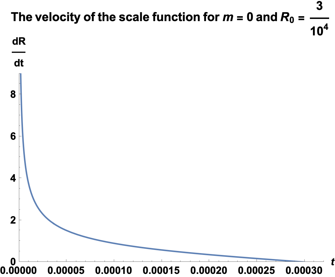
Figure 2: $\frac{dR(t)}{dt}$ from time $t=0$ to $t=R_{0}$. If one considers the today scale function is set $R=1$, the scale function being without unity, we may calibrate time so that, when the radiative forces cease to be the driving one, the corresponding time would be $t=R_{0}$. In the literature we know that the radiation dominated Universe epoch elapsed $\approx 72000years$ [31], page 331.

Having the initial condition to the Bloch vector differential equation

$$\vec{w}(0)=\left(-\frac{R^{2}_{0}}{\lambda},\sqrt{N^{2}-\frac{R^{4}_{0}}{\lambda^{2}}}\sin(\phi_{0}),\sqrt{N^{2}-\frac{R^{4}_{0}}{\lambda^{2}}}\cos(\phi_{0})\right),$$ (46)

and substituting $R(t)$ into (43), and based on the relationship between spherical and hyperbolic trigonometry, we can find the subsequent solutions:

$$\left\{\begin{array}[]{lll}{w}^{1}&=&-\frac{R^{2}_{0}}{\lambda},\\ {w}^{2}&=&-\sqrt{N^{2}-\frac{R^{4}_{0}}{\lambda^{2}}}\sin(4\lambda G(t)),\\ {w}^{3}&=&\sqrt{N^{2}-\frac{R^{4}_{0}}{\lambda^{2}}}\cos\left(4\lambda G(t)\right),\end{array}\right.$$ (50)

where $G(t)=\tan^{-1}\left(\frac{t}{R(t)}\right)$ and $\phi_{0}=0$ . We can notice that the Bloch vector is a function of the scale function $R(t)$.

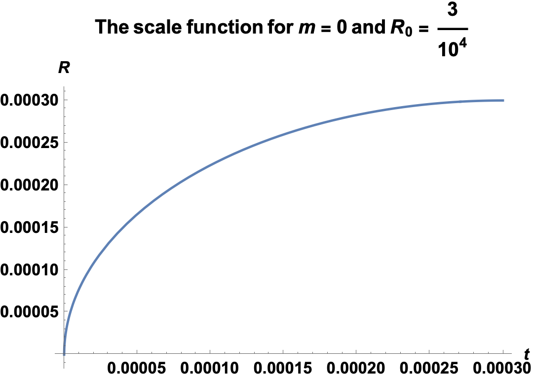
Figure 3: $R(t)$ increasing from time $t=0$ to $t=R_{0}$.

Subtsituting $m=0$ into the components of $\vec{w}$ in (31), (32) and (33), we obtain

$$\left\{\begin{array}[]{lll}{w}^{1}&=&2\text{Re}\left(\alpha\bar{\beta}\right)\\ {w}^{2}&=&2\text{Im}\left(\alpha\bar{\beta}\right)\\ {w}^{3}&=&|\alpha|^{2}-|\beta|^{2}.\end{array}\right.$$ (54)

Replacing $\alpha$ by $\rho_{in_{1}}e^{i\eta_{in_{1}}}$ and $\beta$ by $\rho_{in_{2}}e^{i\eta_{in_{2}}}$ into (54), where $\rho$ is the modulus of $\alpha$ and $\eta$ its argument. We differentiate modulus and arguments from preselected and postselected states with indices. We obtain

$$\left\{\begin{array}[]{lll}{w}^{1}&=&2\rho_{in_{1}}\rho_{in_{2}}\cos(\eta_{in_{1}}-\eta_{in_{2}}),\\ {w}^{2}&=&2\rho_{in_{1}}\rho_{in_{2}}\sin(\eta_{in_{1}}-\eta_{in_{2}}),\\ {w}^{3}&=&\rho_{in_{1}}^{2}-\rho_{in_{2}}^{2}.\end{array}\right.$$ (58)

These results constitute additional constraints for the solutions (50). Consequently ${w}^{1},{w}^{2},{w}^{3}$ must be real numbers. For $G(t)$ to be real, It has to be in the interval $]-\pi/2,\pi/2[$.

From the expression (58) we obtain

$$\eta_{in_{1}}-\eta_{in_{2}} = -\arctan\left(\frac{\sqrt{\lambda^{2}N^{2}-R^{4}_{0}}\sin(4\lambda G(t))}{R^{2}_{0}}\right).$$ (59)

Also from (58) and using the norm from equation (36), we obtain

$$\rho_{in_{1}} =\frac{\sqrt{2}}{2}\sqrt{N+\sqrt{N^{2}-\frac{R^{4}_{0}}{\lambda^{2}}}\cos\left(4\lambda G(t)\right)},$$ (60)

$$\rho_{in_{2}} =\frac{\sqrt{2}}{2}\sqrt{N-\sqrt{N^{2}-\frac{R^{4}_{0}}{\lambda^{2}}}\cos\left(4\lambda G(t)\right)}.$$ (61)

To sum up, $\mid\Psi_{in}\rangle$ is represented by the knowledge of the components of the three-vector $\vec{w}$ or $\alpha_{\text{in}}=\rho_{1}e^{i\eta_{1}}$ and $\beta_{\text{in}}=\rho_{2}e^{i\eta_{2}}$ at a certain $t_{in}$ chosen such that the scale function is real.

For the scale function to be real, $R(t_{in})$ must be real. This implies that $0\leq t_{\text{in}}\leq R_{0}$. Within this period, the scale function increases with time. In our approximation the scale function stops to increase at $R_{0}$. But in the general picture, the driving force due to matter takes over and the Universe continues to expand. Let us point out also that the period within the radiation-dominated Universe is very short compared to the lifespan of the Universe. This period is approximated as $72000$ years vs $13,9$Gyrs today [31]. We also remind that within this period, the scale function is very small. The radiative period ceases where the scale function R approximately attains the value $R\approx 3.10^{-4}$. Finster in [1] shows a bouncing behaviour of the scale function around singularity.

We can illustrate the behaviour of the scale acceleration in the presence of the fermions field. This graphic is constructed only for a Universe without matter.

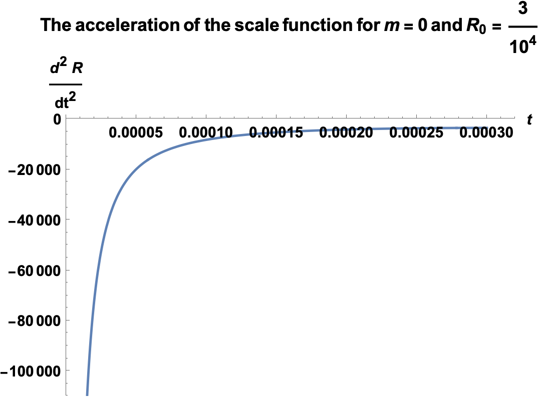
Figure 4: The scale acceleration in the Universe dominated by fermions.

II.2 $\mid\Psi_{out}\rangle$: Solution of the Einstein-Dirac equation for $\lambda=0$.

When $\lambda=0$, the ODEs in (34) becomes:

$$\left\{\begin{array}[]{lll}\dot{w}^{1}&=&0\\ \dot{w}^{2}&=&-2m{w}^{3}\\ \dot{w}^{3}&=&2m{w}^{2},\end{array}\right.$$ (65)

$$\left(\frac{dR}{dt}\right)^{2}+1=-\frac{1}{R}mw^{1}.$$ (66)

We differ from Finster in [1] and we set that at $t_{max},\frac{dR}{dt}|_{t_{max}}=0$, and $R(t_{max})=R_{max}$. This implies that $w^{1}=-\frac{R_{max}}{m}$. One easily sees that the two differential equations decouple. The block vector solution will not depend on the scale function. These equations yield the following solutions

$$R(g) = \frac{R_{max}}{2}\left(1-\cos(g)\right),$$ (67)

$$t(g) = \frac{R_{max}}{2}\left(g-sin\left(g\right)\right),$$ (68)

where g is a parameter varying between $0$ and $2\pi$.

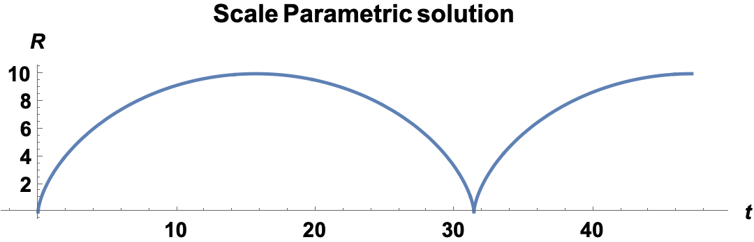
Figure 5: This parametric solution is set for $R_{max}=10$. This value is taken from Finster in [1]. The time is derived from the formula $t(g)=\frac{R_{max}}{2}\left(g-sin\left(g\right)\right)$.

The solution to the Bloch vector differential equation for the following conditions

$$\vec{w}(t_{\text{max}})=\left(w^{1}_{\text{max}},\rho\cos(\phi_{\text{max}}),\rho\sin(\phi_{\text{max}})\right),$$ (69)

gives the following solution:

$$\left\{\begin{array}[]{lll}{w}^{1}&=&-\frac{R_{max}}{m}\\ {w}^{2}&=&\sqrt{N^{2}-\frac{R^{2}_{max}}{m^{2}}}\cos(2mt+\phi_{\text{max}}-2mt_{\text{max}})\\ {w}^{3}&=&\sqrt{N^{2}-\frac{R^{2}_{max}}{m^{2}}}\sin(2mt+\phi_{\text{max}}-2mt_{\text{max}}),\end{array}\right.$$ (73)

where $m$ is the mass of Dirac particle.

Subtsituting $\lambda=0$ into the components of $\vec{w}$ in (31-33), we obtain

$$\left\{\begin{array}[]{lll}{w}^{1}&=&-\left(|\alpha|^{2}-|\beta|^{2}\right)\\ {w}^{2}&=&2\text{Im}\left(\alpha\bar{\beta}\right)\\ {w}^{3}&=&2\text{Re}\left(\alpha\bar{\beta}\right).\end{array}\right.$$ (77)

Replacing $\alpha$ by $\rho_{out_{1}}e^{i\eta_{out_{1}}}$ and $\beta$ by $\rho_{out_{2}}e^{i\eta_{out_{2}}}$ into (54), we obtain

$$\left\{\begin{array}[]{lll}{w}^{1}&=&-\left(\rho_{out_{1}}^{2}-\rho_{out_{2}}^{2}\right)\\ {w}^{2}&=&2\rho_{out_{1}}\rho_{out_{2}}\sin(\eta_{out_{1}}-\eta_{out_{2}})\\ {w}^{3}&=&2\rho_{out_{1}}\rho_{out_{2}}\cos(\eta_{out_{1}}-\eta_{out_{2}}).\end{array}\right.$$ (81)

These results constitute additional constraints for the solutions (50). Consequently ${w}^{1},{w}^{2},{w}^{3}$ must be real numbers.

From the expression (81) we obtain

$$\eta_{out_{1}}-\eta_{out_{2}} = \frac{\pi}{2}-2mt-\phi_{\text{max}}+2mt_{\text{max}}.$$ (82)

We also obtain from (81) and the norm (36):

$$\rho_{out_{1}} =\frac{\sqrt{2}}{2}\sqrt{N+\frac{R_{max}}{m}},$$ (83)

$$\rho_{out_{2}} =\frac{\sqrt{2}}{2}\sqrt{N-\frac{R_{max}}{m}}.$$ (84)

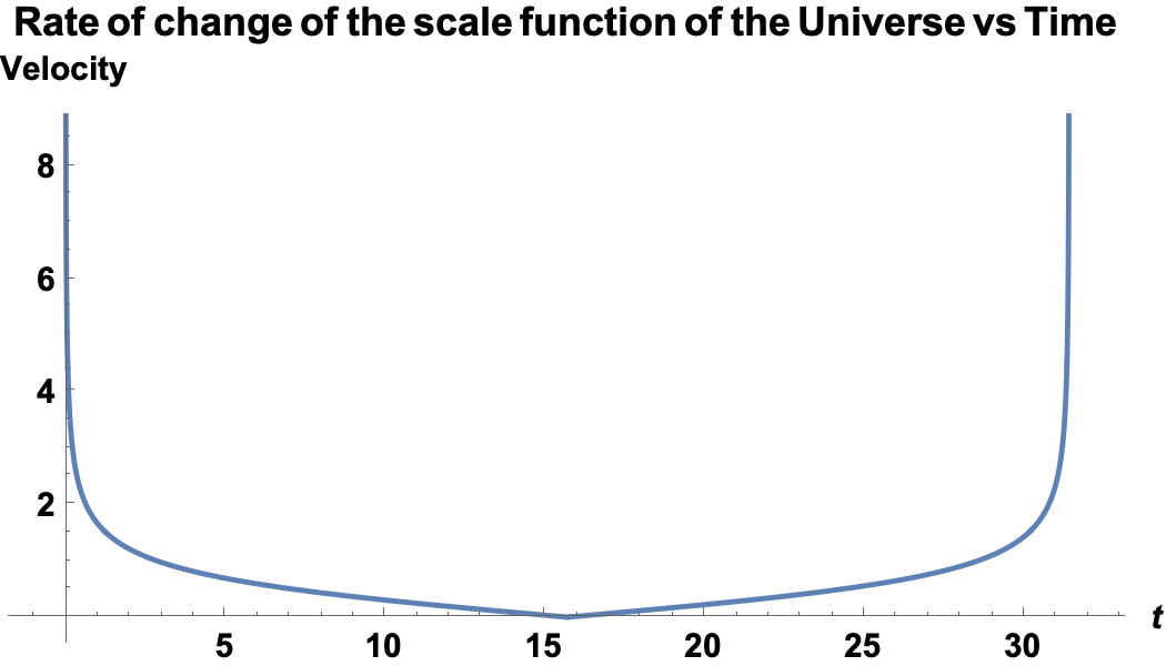
Figure 6: Rate of change the scale function in an Universe dominated by matter.

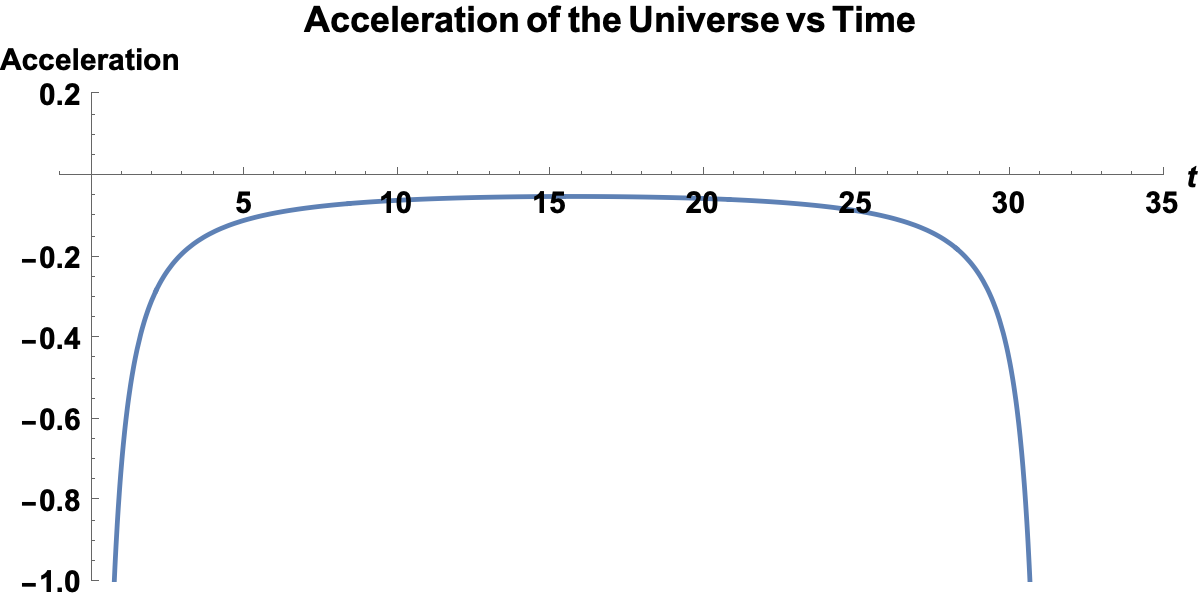
Figure 7: The acceleration of the scale function in an Universe dominated by matter.

To sum up, $\mid\Psi_{out}\rangle$ is represented by the knowledge of the components of the three-vector $\vec{w}$ or $\alpha_{\text{out}}=\rho_{out_{1}}e^{i\eta_{out_{1}}}$ and $\beta_{\text{out}}=\rho_{out_{2}}e^{\eta_{out_{2}}}$ at a certain $t_{out}$ chosen such that the scale function is real.

III Weak measurement on the Einstein-Dirac solutions

The general formula of a weak measurement of any observable is given by

$$\langle\hat{A}\rangle_{w}=\frac{\langle\psi_{out}(t)|\hat{A}|\psi_{in}(t)\rangle}{\langle\psi_{out}(t)|\psi_{in}(t)\rangle}.$$ (85)

wherein, $\langle\psi_{out}(t)|=\langle\psi_{out}(t_{out})|U^{\dagger}(t,t_{out})$ and
$|\psi_{in}(t)\rangle=U(t,t_{in})|\psi_{in}(t_{in})\rangle$.

A pictorial description of a weak measurement in our context is like in figure 8.

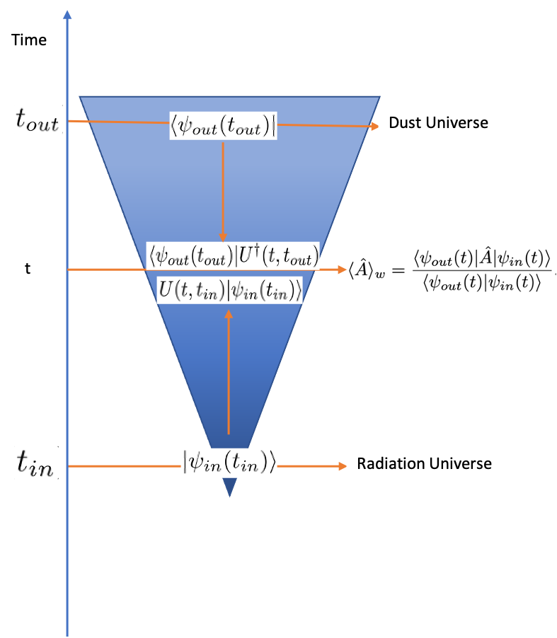
Figure 8: Weak measurement at time t.

The solutions of Einstein-Dirac equation $|\psi_{in}(t_{in})\rangle$ and $|\psi_{out}(t_{out})\rangle$ are defined at the respective times $t_{in}$ and $t_{out}$. We must construct the evolutionary operator to allow the weak measurement to occur at time t between $t_{in}$ and $t_{out}$.

Because of the time dependency of the scale function, an exact evolutionary operator is impossible to compute. Still, it can be approximated by using the Wentzel–Kramers–Brillouin (WKB) method. Following Finster [29], the smallness of the Compton wavelength compared to the lifetime of the Universe justifies the use of WKB-type approximation. Therefore, we define the approximated unitary evolutionary operator as

$$U(t,t_{0})=U^{-1}(t)\left(\begin{array}[]{cc}e^{-iF(t,t_{0})}&0\\ 0&e^{iF(t,t_{0})}\end{array}\right)U(t_{0}).$$ (86)

wherein $F(t,t_{0})=-F(t_{0},t)=\int^{t}_{t_{0}}\frac{\sqrt{R^{2}(t)m^{2}+\lambda^{2}}}{R(t)}dt$.
$U(t)$ is defined such that

$$U(t)\begin{pmatrix}m&-\frac{\lambda}{R(t)}\\ -\frac{\lambda}{R(t)}&-m\end{pmatrix}U(t)^{-1}=\frac{\sqrt{R^{2}(t)m^{2}+\lambda^{2}}}{R(t)}\begin{pmatrix}1&0\\ 0&-1\end{pmatrix}.$$ (87)

The equation (87) yields $g(t)=\frac{1}{2}\arctan(\frac{\lambda}{mR(t)})$ for the unitary matrix given by

$$U(t)=\begin{pmatrix}\cos(g(t))&-\sin(g(t))\\ \sin(g(t))&\cos(g(t))\end{pmatrix}.$$ (88)

The computation of $\left(\begin{array}[]{cc}e^{-iF(t,t_{0})}&0\\ 0&e^{iF(t,t_{0})}\end{array}\right)$ follows Finster in [29].

Let us point out here that $U(t,t_{\text{in}})$ is given by

$$U^{-1}(t)\left(\begin{array}[]{cc}e^{-iF(t,t_{\text{in}})}&0\\ 0&e^{iF(t,t_{\text{in}})}\end{array}\right)U(t_{in})$$

wherein the preselected state is taken from the radiation-dominated Universe with $m=0$, which yields
$g(t_{\text{in}})=\frac{1}{2}\arctan(\frac{\lambda}{m*R(t_{\text{in}})})=\frac{\pi}{4}+k\pi$ for $m=0$. For $k=0$, the matrix will be given by

$$U(t_{\text{in}})=\frac{\sqrt{2}}{2}\begin{pmatrix}1&-1\\ 1&1\end{pmatrix}$$

.

Whereas the postselected state is taken from the dust-dominated Universe wherein $\lambda=0$. This will yield
$g(t)=\frac{1}{2}\arctan(\frac{\lambda}{m*R(t_{\text{in}})})=0+k\pi$ for $\lambda=0$, and for $k=0$ this results in $U(tout)$ is the identity matrix

$$U(t_{out})=\left(\begin{array}[]{cc}1&0\\ 0&1\end{array}\right).$$

Knowing that $\left.U^{\dagger}(t,t_{\text{out}})=U(t_{\text{out}},t)\right.$, this later is given by

$$U^{-1}(t_{\text{out}})\left(\begin{array}[]{cc}e^{-iF(t_{\text{out}},t)}&0\\ 0&e^{iF(t_{\text{out}},t)}\end{array}\right)U(t).$$

The unitary operator approximated, we can now compute the weak measurement of some observable starting from the Energy-momentum Tensor.

III.1 Weak measurement of the Energy-momentum tensor .

In this section, we compute the weak measurement of the energy-momentum tensor given by

$$\langle T_{\mu\nu}\rangle_{w}=\frac{\langle\psi_{out}(t)|T_{\mu\nu}|\psi_{in}(t)\rangle}{\langle\psi_{out}(t)|\psi_{in}(t)\rangle}.$$ (89)

More explicitly, we have

$$\langle T_{\mu\nu}\rangle_{w}=\frac{1}{2}\frac{\langle\psi_{\text{out}}(t)|\left(iG_{\mu}D_{\nu}+iG_{\nu}D_{\mu}\right)|\psi_{\text{in}}(t)\rangle}{\langle\psi_{\text{out}}(t)|\psi_{\text{in}}(t)\rangle}.$$ (90)

where $G^{\mu}$ are the linear combinations of the Dirac matrices of Minkowski space given by:

$$G^{0}=\gamma^{0},$$ (91)

$$G^{r}=\frac{f(r)}{R(t)}\left(\cos\vartheta\gamma^{3}+\sin\vartheta\cos\varphi\gamma^{1}+\sin\vartheta\sin\varphi\gamma^{2}\right),$$ (92)

$$G^{\vartheta}=\frac{1}{rR(t)}\left(-\sin\vartheta\gamma^{3}+\cos\vartheta\cos\varphi\gamma^{1}+\cos\vartheta\sin\varphi\gamma^{2}\right),$$ (93)

$$G^{\varphi}=\frac{1}{rR(t)\sin\vartheta}\left(-\sin\varphi\gamma^{1}+\cos\varphi\gamma^{2}\right),$$ (94)

with $f(r)=\sqrt{1-r^{2}}$. Note that $G_{\mu}=g_{\mu\nu}G^{\nu}$.

The Dirac matrices are given as

$$\gamma^{0}=\begin{pmatrix}I&0\\ 0&-I\end{pmatrix},\quad\gamma^{\alpha}=\begin{pmatrix}0&\sigma^{\alpha}\\ -\sigma^{\alpha}&0\end{pmatrix},$$

where $I$ is the $2\times 2$ identity matrix and $\sigma^{\alpha}$ are the Pauli matrices:

$$\sigma^{1}=\begin{pmatrix}0&1\\ 1&0\end{pmatrix},\quad\sigma^{2}=\begin{pmatrix}0&-i\\ i&0\end{pmatrix},\quad\sigma^{3}=\begin{pmatrix}1&0\\ 0&-1\end{pmatrix}$$

The differential operator is given by $D_{\mu}=\partial_{\mu}-iE_{\mu}\text{, }$ and $G^{\mu}$ obeys to the anti-commutation rule.

$$\left\{G^{\mu},G^{\nu}\right\}\equiv G^{\mu}G^{\nu}+G^{\nu}G^{\mu}=2g^{\mu\nu}\mathbf{1}_{4}.$$

The so-called spin coefficients are given by $E_{\mu}$.

For an orthogonal metric, the combination $G^{\mu}E_{\mu}$ takes the simple form (for more details see [1])

$$G^{\mu}E_{\mu}=\frac{i}{2\sqrt{|g|}}\partial_{\mu}\left(\sqrt{|g|}G^{\mu}\right)\quad\text{ with }\quad g=\operatorname{det}g_{ij},$$

making it unnecessary to compute the spin connection coefficients or even the Christoffel symbols.

To compute the numerator part of the weak measurement of the energy-momentum tensor, following Finster in[29], we adapt the object $P(t,\vec{x};t^{\prime},\vec{x^{\prime}})$ to our need

$$=\left(R(t)R(t^{\prime})\right)^{-\frac{3}{2}}E_{\lambda}(\vec{x},\vec{x^{\prime}})\otimes\begin{pmatrix}\alpha_{\text{in}}(t)\overline{\alpha_{\text{out}}(t^{\prime})}-\alpha_{\text{in}}(t)\overline{\beta_{\text{out}}(t^{\prime})}\\ \beta_{\text{in}}(t)\overline{\alpha_{\text{out}}(t^{\prime})}-\beta_{\text{in}}(t)\overline{\beta_{\text{out}}(t^{\prime})}\end{pmatrix}.$$ (95)

wherein $E_{\lambda}$ denote the spectral projectors of $\mathcal{D}_{S^{3}}$, given by $E_{\pm\mid\lambda\mid}=\displaystyle\sum^{\mid\lambda\mid-\frac{3}{2}}_{n=0}\sum^{j}_{k=-j}\psi^{\pm}_{njk}(x)\overline{\psi^{\pm}_{njk}(\acute{x})}$. Then, the numerator part of the energy-momentum tensor, $\langle\psi_{\text{out}}|T_{\mu\nu}|\psi_{\text{in}}\rangle(t,\vec{x})$ can be expressed in terms of $P$ by

$$\begin{split}=\frac{1}{2}\operatorname{Tr}_{\mathbb{C}^{4}}\Big{\{}&\left(iG_{\mu}D_{\nu}+iG_{\nu}D_{\mu}\right)P\left(t,\vec{x};t^{\prime},\vec{x}^{\prime}\right)\Big{\}}\Bigg{|}_{t^{\prime}=t,\vec{x}^{\prime}=\vec{x}}.\end{split}$$ (96)

Because of the homogeneity and the isotropy of the FLRW space, only the diagonal energy-momentum tensor components are different from 0. We get the following results after computations and normalization

$$\langle T_{0}^{0}\rangle_{w}=\frac{\langle\psi_{out}(t)|T_{0}^{0}|\psi_{in}(t)\rangle}{\langle\psi_{out}(t)|\psi_{in}(t)\rangle}=\frac{\Bigl{[}mR(t)\left(\alpha_{\text{in}}(t)\overline{\alpha_{\text{out}}}(t)-\beta_{\text{in}}(t)\overline{\beta_{\text{out}}}(t)\right)-\lambda\left(\alpha_{\text{in}(t)}\overline{\beta_{\text{out}}}(t)+\beta_{\text{in}}(t)\overline{\alpha_{\text{out}}}(t)\right)\Bigr{]}}{R(t)\left(\overline{\alpha_{\text{out}}}(t)\alpha_{\text{in}}(t)+\overline{\beta_{\text{out}}}(t)\beta_{\text{in}}(t)\right)},$$ (97)

and

$$\langle T_{j}^{j}\rangle_{w}=\frac{\langle\psi_{out}(t)|T_{j}^{j}|\psi_{in}(t)\rangle}{\langle\psi_{out}(t)|\psi_{in}(t)\rangle}=\frac{\lambda\left(\alpha_{\text{in}}(t)\overline{\beta_{\text{out}}}(t)+\beta_{\text{in}}(t)\overline{\alpha_{\text{out}}}(t)\right)}{3R(t)\left(\overline{\alpha_{\text{out}}}(t)\alpha_{\text{in}}(t)+\overline{\beta_{\text{out}}}(t)\beta_{\text{in}}(t)\right)},$$ (98)

where j represents $r,\vartheta,\varphi$. Due to spherical symmetry and homogeneity of the space, $T_{r}^{r}=T_{\vartheta}^{\vartheta}=T_{\varphi}^{\varphi}$ are all equal.

One sees here that if $|\psi_{in}(t)\rangle=|\psi_{out}(t)\rangle$, the weak measurement of the energy-momentum tensor will coincide with the one computed in [1]. In this regard, weak measurements are generalizations of classical ones.

Another quick observation is that if

$$\overline{\alpha_{\text{out}}}(t)\alpha_{\text{in}}(t)+\overline{\beta_{\text{out}}}(t)\beta_{\text{in}}(t)\approx 0,$$

an amplification phenomenon occurs. This is realized when $\overline{\alpha_{\text{out}}}(t)\approx-k\beta_{\text{in}}(t)$ and $\overline{\beta_{\text{out}}}(t)\approx k\alpha_{\text{in}}(t)$, where $k$ is a factor or a phase.

For better analysis, we construct a complex Bloch vector since it is constructed in the same manner as a Bloch vector, but the components are complex functions. Aharonov and Gruss constructed a density operator from the Two-State vectors in their paper Two-time interpretations of quantum mechanic [9]. This complex Bloch vector is linked to that density operator. One should note that if the preselected state is equal to the postselected one, then we shall get the same construction as in the paper of Finster and Hainzl on page 14 in [1].

$$\vec{v}_{f,i}=\begin{pmatrix}v_{f,i}^{1}\\ v_{f,i}^{2}\\ v_{f,i}^{3}\end{pmatrix}=\begin{pmatrix}\langle\xi_{\text{out}}(t)|\sigma^{1}|\xi_{\text{in}}(t)\rangle\\ \langle\xi_{\text{out}}(t)|\sigma^{2}|\xi_{\text{in}}(t)\rangle\\ \langle\xi_{\text{out}}(t)|\sigma^{3}|\xi_{\text{in}}(t)\rangle\end{pmatrix}$$

wherein $\xi_{\text{out}}(t)=\left(\begin{array}[]{c}\alpha_{\text{out}}(t)\\ \beta_{\text{out}}(t)\end{array}\right)$ and $\xi_{\text{in}}(t)=\left(\begin{array}[]{c}\alpha_{\text{in}}(t)\\ \beta_{\text{in}}(t)\end{array}\right)$.

We also define $v_{f,i}^{0}$ as $\langle\xi_{\text{out}}(t)|I_{2\times 2}|\xi_{\text{in}}(t)\rangle$ where $I_{2\times 2}$ is the 2 dimensional identity matrix. This will yield $\overline{\alpha_{\text{out}}}(t)\alpha_{\text{in}}(t)+\overline{\beta_{\text{out}}}(t)\beta_{\text{in}}(t)$.
We can now redefine the weak energy-momentum tensor as

$$\begin{split}&\langle T_{0}^{0}\rangle_{w}=\frac{\Bigl{[}mR(t)\left(v_{f,i}^{3}\right)-\lambda\left(v_{f,i}^{1}\right)\Bigr{]}}{R(t)\left(v_{f,i}^{0}\right)}\\ &\langle T_{j}^{j}\rangle_{w}=\frac{\lambda\left(v_{f,i}^{1}\right)}{3R(t)\left(v_{f,i}^{0}\right)}\end{split}$$ (99)

Let us express the energy-momentum tensor weak values in terms of $\alpha_{\text{in}}(t_{\text{in}})$ and $\alpha_{\text{out}}(t_{\text{out}})$ wherein
$A=e^{i\left(F(t_{\text{out}},t_{\text{in}})\right)}$, $\bar{A}=e^{-i\left(F(t_{\text{out}},t_{\text{in}})\right)}$,
$B=e^{i\left(F(t,t_{\text{in}})+F(t,t_{\text{out}})\right)}$ and $\bar{B}=e^{-i\left(F(t,t_{\text{in}})+F(t,t_{\text{out}})\right)}$. Because of the lengthiness of the expression, we break it as follows

$$\begin{split}&v_{f,i}^{0}=\frac{\sqrt{2}}{2}\left(\overline{\alpha_{\text{out}}}(t_{\text{out}})\alpha_{\text{in}}(t_{\text{in}})-\overline{\alpha_{\text{out}}}(t_{\text{out}})\beta_{\text{in}}(t_{\text{in}})\right)\bar{A}+\frac{\sqrt{2}}{2}\left(\overline{\beta_{\text{out}}}(t_{\text{out}})\beta_{\text{in}}(t_{\text{in}})+\overline{\beta_{\text{out}}}(t_{\text{out}})\alpha_{\text{in}}(t_{\text{in}})\right)A,\end{split}$$ (100)

$$\begin{split}&v_{f,i}^{3}=\frac{\sqrt{2}}{2}\alpha_{\text{in}}(t_{\text{in}})\overline{\alpha_{\text{out}}}(t_{\text{out}})\left[\sin{(2g(t))}B+\cos{(2g(t))}\bar{A}\right]+\frac{\sqrt{2}}{2}\beta_{\text{in}}(t_{\text{in}})\overline{\beta_{\text{out}}}(t_{\text{out}})\left[-\sin{(2g(t))}\bar{B}-\cos{(2g(t))}A\right]\\ &+\frac{\sqrt{2}}{2}\alpha_{\text{in}}(t_{\text{in}})\overline{\beta_{\text{out}}}(t_{\text{out}})\left[\sin{(2g(t))}\bar{B}-\cos{(2g(t))}A\right]+\frac{\sqrt{2}}{2}\beta_{\text{in}}(t_{\text{in}})\overline{\alpha_{\text{out}}}(t_{\text{out}})\left[\sin{(2g(t))}B-\cos{(2g(t))}\bar{A}\right],\end{split}$$ (101)

$$\begin{split}&v_{f,i}^{1}=\frac{\sqrt{2}}{2}\alpha_{\text{in}}(t_{\text{in}})\overline{\alpha_{\text{out}}}(t_{\text{out}})\left[-\sin{(2g(t))}\bar{A}+\cos{(2g(t))}B\right]+\frac{\sqrt{2}}{2}\beta_{\text{in}}(t_{\text{in}})\overline{\beta_{\text{out}}}(t_{\text{out}})\left[\sin{(2g(t))}A-\cos{(2g(t))}\bar{B}\right]\\ &+\frac{\sqrt{2}}{2}\alpha_{\text{in}}(t_{\text{in}})\overline{\beta_{\text{out}}}(t_{\text{out}})\left[\sin{(2g(t))}A+\cos{(2g(t))}\bar{B}\right]+\frac{\sqrt{2}}{2}\beta_{\text{in}}(t_{\text{in}})\overline{\alpha_{\text{out}}}(t_{\text{out}})\left[\sin{(2g(t))}\bar{A}+\cos{(2g(t))}B\right].\end{split}$$ (102)

We can deduce the orthogonality condition for $v_{f,i}^{0}\approx 0$. This is obtained if $\overline{\alpha_{\text{out}}}(t_{\text{out}})\approx$:

$$\begin{split}&-\frac{\sqrt{2}}{2}\alpha_{\text{in}}(t_{\text{in}})\left[-\sin{(g(t_{\text{out}}))}e^{-iF(t_{\text{out}},t_{\text{in}})}+\cos{(g(t_{\text{out}}))}e^{iF(t_{\text{out}},t_{\text{in}})}\right]\\ &-\frac{\sqrt{2}}{2}\beta_{\text{in}}(t_{\text{in}})\left[\sin{(g(t_{\text{out}}))}e^{-iF(t_{\text{out}},t_{\text{in}})}+\cos{(g(t_{\text{out}}))}e^{iF(t_{\text{out}},t_{\text{in}})}\right].\end{split}$$ (103)

and $\overline{\beta_{\text{out}}}(t_{\text{out}})\approx$

$$\begin{split}&\frac{\sqrt{2}}{2}\alpha_{\text{in}}(t_{\text{in}})\left[\cos{(g(t_{\text{out}}))}e^{-iF(t_{\text{out}},t_{\text{in}})}+\sin{(g(t_{\text{out}}))}e^{iF(t_{\text{out}},t_{\text{in}})}\right]\\ &+\frac{\sqrt{2}}{2}\beta_{\text{in}}(t_{\text{in}})\left[-\cos{(g(t_{\text{out}}))}e^{-iF(t_{\text{out}},t_{\text{in}})}+\sin{(g(t_{\text{out}}))}e^{iF(t_{\text{out}},t_{\text{in}})}\right].\end{split}$$ (104)

As it is difficult to have a simple expression of the weak measurement of the energy-momentum tensor to make an interpretation, let us compute a concrete example with values that make the computation easy. Let us consider $\lambda=3/2$, the eigenvalue of the Dirac operator $\mathcal{D}_{\mathcal{H}}$, $t_{\text{in}}\approxeq 0$ and $R_{0}=10^{-3}$. Theses conditions imply $G(t_{\text{in}})=0$ in (50). They will yield the following expression: $\rho_{in_{1}}\approx 2$ and $\rho_{in_{2}}\approx 0$ and $\eta_{in_{1}}-\eta_{in_{2}}=0$. For simplicity, we shall consider $\eta_{in_{1}}=\eta_{in_{2}}=0$.

We also remind that the preselected state is taken from the radiation-dominated Universe with $m=0$ which yields $g(t_{\text{in}})=\frac{1}{2}\arctan(\frac{\lambda}{0*R(t_{\text{in}})})=\frac{\pi}{4}+k\pi$. For $k=0$, the matrix will be given by $U(t_{\text{in}})=\frac{\sqrt{2}}{2}\begin{pmatrix}1&-1\\ 1&1\end{pmatrix}$. Therefore the preselected state at $t_{\text{in}}$ will be $\alpha_{\text{in}}(t_{\text{in}})=2$ and $\beta_{\text{in}}(t_{\text{in}})=0$.

As for the postselected state vector, the scale function and the time expressed $R(g)=\frac{R_{\text{max}}}{2}\left(1-\cos(g)\right)$, $t(g)=\frac{R_{\text{max}}}{2}\left(g-\sin(g)\right)$, we have the following observations

• A maximal $R(g)$ will be $R_{\text{max}}$, and the maximal $t$, that is $t_{\text{out}}$ will be $R_{\text{max}}k\frac{\pi}{2}$.

• We shall have: $\rho_{\text{out}1}=\sqrt{2+\frac{R_{\text{max}}}{m}}$,     $\rho_{\text{out}2}=\sqrt{2-\frac{R_{\text{max}}}{m}}$ and $\eta_{\text{out}1}-\eta_{\text{out}2}=\frac{\pi}{2}-\phi_{\text{max}}$.

We remind that the postselected state is taken from the dust-dominated Universe wherein $\lambda=0$. This will yield $g(t)=\frac{1}{2}\arctan(\frac{0}{m*R(t_{\text{in}})})=0+k\pi$ . This will lead, for $k=0$, to $U(t_{out})=\left(\begin{array}[]{cc}1&0\\ 0&1\end{array}\right)$, an identity matrix.

The postselected state $t_{\text{out}}$ will be

$$\begin{split}&\alpha_{\text{out}}(t_{\text{out}})=\sqrt{2+\frac{R_{\text{max}}}{m}}e^{i\left(\frac{\pi}{2}-\phi_{\text{max}}\right)},\\ &\beta_{\text{out}}(t_{\text{out}})=\sqrt{2-\frac{R_{\text{max}}}{m}}.\end{split}$$ (105)

For simplicity, let us consider a weak measurement taking place at $t=t_{out}$ Universe and $R_{\text{max}}=10$ and $m=21.5$. This implies that

$$\left.\left(\begin{array}[]{c}\alpha_{\text{in}}(t_{\text{out}})\\ \beta_{\text{in}}(t_{\text{out}})\end{array}\right)=U(t_{\text{out}},t_{\text{in}})\left(\begin{array}[]{c}\alpha_{\text{in}}(t_{\text{in}})\\ \beta_{\text{in}}(t_{\text{in}})\end{array}\right)\right.,$$

where

$$U(t_{\text{out}},t_{\text{in}})=\frac{1}{\sqrt{2}}\left(\begin{array}[]{cc}e^{-i\pi m\text{Rmax}}&-e^{-i\pi m\text{Rmax}}\\ e^{i\pi m\text{Rmax}}&e^{i\pi m\text{Rmax}}\\ \end{array}\right),$$

and $U(t_{\text{out}},t_{\text{out}})=I$. $F(t_{\text{out}},t_{\text{in}})=mt_{\text{out}}$. These elements yield the following state vectors

$$\begin{split}&\alpha_{\text{in}}(t_{\text{out}})=\frac{1}{\sqrt{2}}(\alpha_{\text{in}}-\beta_{\text{in}})e^{-i\pi m\text{Rmax}},\\ &\beta_{\text{in}}(t_{\text{out}})=\frac{1}{\sqrt{2}}(\alpha_{\text{in}}+\beta_{\text{in}})e^{i\pi m\text{Rmax}}.\end{split}$$ (106)

Since the weak measurement is taking place at $t=t_{\text{out}}$, the postselected stated is fixed.

The values in the weak measurement of the energy-momentum tensor in the following expression

$$\begin{split}&\langle T_{0}^{0}\rangle_{w}=\frac{\Bigl{[}mR(t_{\text{out}})\left(v_{f,i}^{3}\right)-\lambda\left(v_{f,i}^{1}\right)\Bigr{]}}{R(t_{\text{out}})\left(v_{f,i}^{0}\right)}\\ &\langle T_{j}^{j}\rangle_{w}=\frac{\lambda\left(v_{f,i}^{1}\right)}{3R(t_{\text{out}})\left(v_{f,i}^{0}\right)}\end{split}$$ (107)

will be:

$$\begin{split}&v_{f,i}^{0}=1.6e^{i\pi mR_{\text{max}}}-(2.3i)e^{i\phi_{\text{max}}-i\pi mR_{\text{max}}}\\ &v_{f,i}^{1}=(2.3i)e^{i(\pi mR_{\text{max}}+\phi_{\text{max}})}+1.6e^{-i\pi mR_{\text{max}}}\\ &v_{f,i}^{3}=(2.3i)\left(-e^{i\phi_{\text{max}}-i\pi mR_{\text{max}}}\right)-1.6e^{i\pi mR_{\text{max}}}\end{split}$$ (108)

What we can conclude is that weak measurements reveal unusual values, such as complex numbers. In our case, for fixed $m$ and $R_{\text{max}}$, the numerical result will depend on $\phi_{max}$.

In (24) the acceleration of the Universe is given in terms of the energy momentum tensor. In (29), the acceleration of the Universe is given in terms of the Bloch vector. But in the Two-State Formalism, the Hopf transformation yields a complex Bloch vector. The Two-State Formalism generalizes the One-State Formalism since it suffices to consider the same state vector in the Two-State Formalism to have the classical Bloch vector. We propose to give here the acceleration of the universe in terms of weak measurements of the energy-momentum tensors and derive it in terms of Complex Bloch vector. The acceleration of the Universe would then be given as

$$\begin{split}\ddot{R}&=\frac{R}{2}\left(3\langle T_{j}^{j}\rangle_{w}-\langle T_{0}^{0}\rangle_{w}\right),\\ \ddot{R}&=\frac{\Bigl{[}-mR\left(v_{f,i}^{3}\right)+2\lambda\left(v_{f,i}^{1}\right)\Bigr{]}}{2\left(v_{f,i}^{0}\right)}.\end{split}$$ (109)

In this formula, one clearly sees that the acceleration of the Universe may be comprehended from the Two-State Formalism and weak measurements theories. Assuming a different postselected state vector may change the shape of the acceleration of the Universe. We remind here that the real and the imaginary parts of a weak value can be measured. The real part of a weak value may be interpreted as the conditioned average associated with an observable in Two Vector Formalism, [24], [32], and they represent the shift of the average detected position due to postselection. The imaginary part of the weak value represents the shift of the average impulsion due to postselection.

The computation of the acceleration of the Universe with the above condition would yield

$$\begin{split}&\ddot{R}=Re\left(\frac{\Bigl{[}-mR\left(v_{f,i}^{3}\right)+2\lambda\left(v_{f,i}^{1}\right)\Bigr{]}}{2\left(v_{f,i}^{0}\right)}\right)\end{split}$$ (110)

This example shows that the acceleration is not Zero and depends here on the postselection.

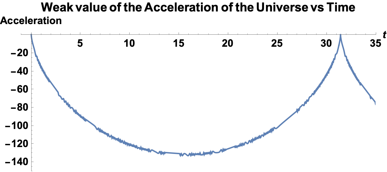
Figure 9: The real part of the weak values of the acceleration of the Universe in function of time for $m=21.5,R_{\text{max}}=10,\phi_{\text{max}}=0$ and $\lambda=\frac{3}{2}$

Figure (9) is about the weak measurement of the acceleration of the Universe as a function of time in a matter Dominated Universe.

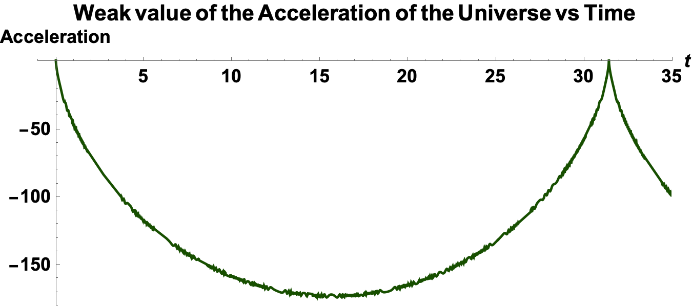
Figure 10: The real part of the weak values of the acceleration of the Universe in function of time for $m=21,R_{\text{max}}=10,\phi_{\text{max}}=\frac{\pi}{4}$ and $\lambda=\frac{3}{2}$.

The difference between Figure 9 and 10 shows how the acceleration of the Universe may change with a different postselection. We have postselected a state vector with $\phi_{\text{max}}=0$ in Figure 9 and $\phi_{\text{max}}=\frac{\pi}{4}$ in Figure 10. It is clear that, this difference causes more acceleration in Figure 10 than in Figure 9. In conclusion, we have shown how to compute the weak measurement of the Energy-momentum tensor. We derived how to amplify weak values of the energy-momentum tensor using an appropriate state vector almost orthogonal to the preselected one. We have finally derived the weak values of the acceleration of the Universe and have showed how sensitive it is compared to classical acceleration.

III.2 Weak measurement of $\sigma^{z}$ operator.

In this section, we delve into the weak measurement of the $\sigma^{z}$ operator which is given by the following expression

$$\sigma^{z}_{w}=\frac{\langle\psi_{out}(t)|\sigma^{z}|\psi_{in}(t)\rangle}{\langle\psi_{out}(t)|\psi_{in}(t)\rangle}.$$ (111)

Following Kofman, Cormann and Ferraz in [33], [34] and [7] respectively, the weak measurement of the generator of $SU(2)$ is given by

$$\sigma_{r,w}=\frac{\vec{f}.\vec{r}+\vec{r}.\vec{i}+i\vec{f}.(\vec{r}\wedge\vec{i})}{\frac{1}{2}(1+\vec{f}.\vec{i})}.$$ (112)

In our case, $\vec{r}=(\begin{array}[]{ccc}0&0&1\end{array})$ to get $\sigma^{z}$. Following Kofman in [33], the vectors $\vec{f}$ and $\vec{i}$ are computed as follows

$$\vec{w_{f}}=\begin{pmatrix}\langle\xi_{\text{out}}(t)|\sigma^{1}|\xi_{\text{out}}(t)\rangle\\ \langle\xi_{\text{out}}(t)|\sigma^{2}|\xi_{\text{out}}(t)\rangle\\ \langle\xi_{\text{out}}(t)|\sigma^{3}|\xi_{\text{out}}(t)\rangle\end{pmatrix},$$

where $\xi_{\text{out}}(t)=\left(\begin{array}[]{c}\alpha_{\text{out}}(t)\\ \beta_{\text{out}}(t)\end{array}\right)$ is expressed as

$$\begin{split}\overline{\alpha_{\text{out}}}(t)=&\overline{\alpha_{\text{out}}}(t_{\text{out}})\cos{(g(t))}e^{-iF(t_{\text{out}},t)}+\\ &\overline{\beta_{\text{out}}}(t_{\text{out}})\sin{(g(t))}e^{iF(t_{\text{out}},t)},\end{split}$$ (113)

and

$$\begin{split}\overline{\beta_{\text{out}}}(t)=&-\overline{\alpha_{\text{out}}}(t_{\text{out}})\sin{(g(t))}e^{-iF(t_{\text{out}},t)}+\\ &\overline{\beta_{\text{out}}}(t_{\text{out}})\cos{(g(t))}e^{iF(t_{\text{out}},t)}.\end{split}$$ (114)

In the same way, the preselected state is given by:

$$\vec{w_{i}}=\begin{pmatrix}\langle\xi_{\text{in}}(t)|\sigma^{1}|\xi_{\text{in}}(t)\rangle\\ \langle\xi_{\text{in}}(t)|\sigma^{2}|\xi_{\text{in}}(t)\rangle\\ \langle\xi_{\text{in}}(t)|\sigma^{3}|\xi_{\text{in}}(t)\rangle\end{pmatrix},$$

where $\xi_{\text{in}}(t)=\left(\begin{array}[]{c}\alpha_{\text{in}}(t)\\ \beta_{\text{in}}(t)\end{array}\right)$ is expressed as

$$\begin{split}\alpha_{\text{in}}(t)=&\frac{\sqrt{2}}{2}\alpha_{\text{in}}(t_{\text{in}})\left[\cos{(g(t))}e^{-iF(t,t_{\text{in}})}+\sin{(g(t))}e^{iF(t,t_{\text{in}})}\right]+\\ &\frac{\sqrt{2}}{2}\beta_{\text{in}}(t_{\text{in}})\left[-\cos{(g(t))}e^{-iF(t,t_{\text{in}})}+\sin{(g(t))}e^{iF(t,t_{\text{in}})}\right],\end{split}$$ (115)

and

$$\begin{split}\beta_{\text{in}}(t)=&\frac{\sqrt{2}}{2}\alpha_{\text{in}}(t_{\text{in}})\left[-\sin{(g(t))}e^{-iF(t,t_{\text{in}})}+\cos{(g(t))}e^{iF(t,t_{\text{in}})}\right]+\\ &\frac{\sqrt{2}}{2}\beta_{\text{in}}(t_{\text{in}})\left[\sin{(g(t))}e^{-iF(t,t_{\text{in}})}+\cos{(g(t))}e^{iF(t,t_{\text{in}})}\right].\end{split}$$ (116)

For simplicity we shall consider $t_{\text{in}}=0$ which implies that $\eta_{\text{in1}}-\eta_{\text{in2}}=0$. We will set $\eta_{in_{1}}-\eta_{in_{2}}=\Delta_{in}$ when necessary. This implies $\Delta_{\text{in}}=0$ and $t_{\text{out}}=t_{\text{max}}$. We obtain the following Postselected and Preselected vectors $\vec{w_{f}}$ and $\vec{w_{i}}$ whose components are given as $\vec{w_{f}}=$

$$\left\{\begin{array}[]{lll}&{w_{f}}^{1}=-\frac{R_{\text{max}}}{m}\sin{(2g(t))}+\\ &\sqrt{N^{2}-\frac{R^{2}_{max}}{m^{2}}}\cos{\left(\frac{\pi}{2}-\phi_{\text{max}}-2F(t_{\text{out}},t)\right)}\cos{(2g(t))}\\ &{w_{f}}^{2}=\sqrt{N^{2}-\frac{R^{2}_{max}}{m^{2}}}\sin{(\frac{\pi}{2}-\phi_{\text{max}}-(2F(t_{\text{out}},t)))}\\ &{w_{f}}^{3}=\frac{R_{\text{max}}}{m}\cos{(2g(t))}+\\ &\sqrt{N^{2}-\frac{R^{2}_{max}}{m^{2}}}\cos{(\frac{\pi}{2}-\phi_{\text{max}}-2F(t_{\text{out}},t))}\sin{(2g(t))}\\ \end{array}\right.,$$ (122)

and $\vec{w_{i}}=$

$$\left\{\begin{array}[]{lll}w_{i}^{1}&=&\sqrt{N^{2}-\frac{R_{0}^{4}}{\lambda^{2}}}\cos{(2g(t))}\cos{(2F(t,t_{\text{in}}))}+\frac{R_{0}^{2}}{\lambda}\sin{(2g(t))}\\ w_{i}^{2}&=&-\sqrt{N^{2}-\frac{R_{0}^{4}}{\lambda^{2}}}\sin{(2F(t,t_{\text{in}}))}\\ w_{i}^{3}&=&\sqrt{N^{2}-\frac{R_{0}^{4}}{\lambda^{2}}}\sin{(2g(t))}\cos{(2F(t,t_{\text{in}}))}-\frac{R_{0}^{2}}{\lambda}\cos{(2g(t))}\end{array}\right..$$ (126)

The vector $\vec{f}$ is equal to $\frac{\vec{w_{f}}}{|\vec{w_{f}}|},\text{and }\vec{i}=\frac{\vec{w_{i}}}{|\vec{w_{i}}|}$. The length of both Bloch vectors are

$$|\vec{w_{f}}|=|\vec{w_{i}}|=\lambda^{2}-\frac{1}{4}.$$

They represent the unit vectors on the Bloch sphere of post-selected and pre-selected state. In terms of the components, the $\sigma^{z}$ weak measurement is given by

$$\sigma_{r,w}=\frac{{w_{f}}^{3}+{w_{i}}^{3}+i(-{w_{f}}^{1}{w_{i}}^{2}+{w_{f}}^{2}{w_{i}}^{1})}{\frac{1}{2}(1+{w_{f}}^{1}{w_{i}}^{1}+{w_{f}}^{2}{w_{i}}^{2}+{w_{f}}^{3}{w_{i}}^{3})}.$$ (127)

The real part of the numerator of the weak value of $\sigma^{z}$ operator in general terms with the above conditions ($t_{\text{in}}=0$, $\Delta_{\text{in}}=0$ and $t_{\text{out}}=t_{\text{max}}$), $\sigma_{r,w}$, is given by

${w_{f}}^{3}+{w_{i}}^{3}=$

$$\begin{split}&\sin(2g(t))\left(\Delta\rho_{\text{in}}^{2}\cos\left(2F\left(t,t_{\text{in}}\right)\right)+2\rho_{out_{1}}\rho_{out_{2}}\cos\left(\Delta_{\text{out}}\right)\right)+\\ &\left(\Delta\rho_{\text{out}}^{2}-2\rho_{in_{1}}\rho_{in_{2}}\right)\cos(2g(t)).\end{split}$$ (128)

In terms of the preselected and postselected we have computed, it would be

$$\begin{split}&\sqrt{N^{2}-\frac{R_{0}^{4}}{\lambda^{2}}}\cos\left(2F\left(t,t_{\text{in}}\right)\right)\sin(2g(t))+\frac{\left(-mR_{0}^{2}+\lambda R_{\max}\right)\cos(2g(t))}{m\lambda}+\\ &\sqrt{N^{2}-\frac{R_{\max}^{2}}{m^{2}}}\sin(2g(t))\sin\left(2F\left(t_{\text{out}},t\right)+\phi_{\max}\right).\end{split}$$ (129)

In the same way, the imaginary part of the numerator of the weak value of $\sigma^{z}$ operator is expressed, in general term with the above conditions as,

$-{w_{f}}^{1}{w_{i}}^{2}+{w_{f}}^{2}{w_{i}}^{1}=$

$$\begin{split}&2\rho_{out_{1}}\rho_{out_{2}}\left(\Delta\rho_{\text{in}}^{2}\cos(2g(t))\sin\left(2F\left(t,t_{\text{in}}\right)+\Delta_{\text{out}}\right)+\right.\\ &\left.\rho_{in_{1}}\rho_{in_{2}}\sin(2g(t))\sin\left(\Delta_{\text{out}}\right)\right)-\Delta\rho_{\text{in}}^{2}\Delta\rho_{\text{out}}^{2}\sin(2g(t))\sin\left(2F\left(t,t_{\text{in}}\right)\right).\end{split}$$ (130)

It would explicitly be given in terms of the preselected and postselected state as

$$\begin{split}&-\frac{\sin\left(2F\left(t,t_{\text{in}}\right)\right)\sin(2g(t))\sqrt{N^{2}-\frac{R_{0}^{4}}{\lambda^{2}}}R_{\max}}{m}+\\ &\frac{1}{\lambda}\sqrt{N^{2}-\frac{R_{\max}^{2}}{m^{2}}}\left(R_{0}^{2}\cos\left(2F\left(t_{\text{out}},t\right)+\phi_{\max}\right)\sin(2g(t))+\right.\\ &\left.\lambda\sqrt{N^{2}-\frac{R_{0}^{4}}{\lambda^{2}}}\cos(2g(t))\cos\left(2F\left(t,t_{\text{in}}\right)-2F\left(t_{\text{out}},t\right)-\phi_{\max}\right)\right).\end{split}$$ (131)

Finally, the denominator part will be given in general terms by:
$(1+{w_{f}}^{1}{w_{i}}^{1}+{w_{f}}^{2}{w_{i}}^{2}+{w_{f}}^{3}{w_{i}}^{3})=$

$$\begin{split}&2\Delta\rho_{\text{in}}^{2}\rho_{out_{1}}\rho_{out_{2}}\cos\left(2F\left(t,t_{\text{in}}\right)+\Delta_{\text{out}}\right)-2\Delta\rho_{\text{out}}^{2}\rho_{in_{1}}\rho_{in_{2}}+1.\end{split}$$ (132)

It would explicitly be given by:

$$\begin{split}&\sqrt{N^{2}-\frac{R_{0}^{4}}{\lambda^{2}}}\sqrt{N^{2}-\frac{R_{\max}^{2}}{m^{2}}}\cos\left(a\right)-\frac{R_{0}^{2}R_{\max}}{\lambda m}+1\end{split}.$$ (133)

wherein $a=2F\left(t,t_{\text{in}}\right)+\Delta_{\text{out}}$.

One can see that the amplification phenomenon is obtained in many ways. One way is

$$\begin{split}\cos(a)\approx-\frac{1-\frac{R_{0}^{2}R_{\max}}{\lambda m}}{\sqrt{N^{2}-\frac{R_{0}^{4}}{\lambda^{2}}}\sqrt{N^{2}-\frac{R_{\max}^{2}}{m^{2}}}}\end{split}.$$ (134)

We remind that $\Delta_{\text{out}}=(\eta_{out_{1}}-\eta_{out_{2}}+2F(t_{\text{out}},t))$. By adjusting adequately the parameters appearing in $a$, one can amplify the weak values.

It is essential to note that any arbitrary observable in a 2-level system can be expressed as $\hat{A}=a_{I}\hat{I}_{2}+a_{L}\vec{\alpha}.\hat{\vec{\sigma}}$, where $a_{I}$ and $a_{L}$ are constants, $\vec{\alpha}$ is a unit vector in three dimensions, and $\sigma$ denotes the Pauli matrices.

In this subsection we have derived the computation of the weak value of the Z component of the Spin of fermions in the context of cosmology. We have shown how it is possible to amplify the signal by choosing adequate parameters.

III.3 Berry phase from the weak measurement of a pure state.

Let us now compute the weak measurement of a pure state which is given as:

$$\hat{\Pi}_{r,w}=\frac{\langle\psi_{out}(t)|\hat{\Pi}_{r}|\psi_{in}(t)\rangle}{\langle\psi_{out}(t)|\psi_{in}(t)\rangle}.$$ (135)

where $\hat{\Pi}_{r}$ is a pure state given as $\frac{1}{2}\left(\hat{I}+\vec{r}\vec{\hat{\sigma}}\right)$. The complete formula to compute the weak values of a pure state is found in [33] or the appendix of [34] and [7]. It reads as

$$\hat{\Pi}_{r,w}=\frac{1+\vec{f}.\vec{r}+\vec{r}.\vec{i}+\vec{f}.\vec{i}+i\vec{f}.(\vec{r}\wedge\vec{i})}{\frac{1}{2}(1+\vec{f}.\vec{i})}.$$ (136)

The vector $\vec{r}$ is defined as

$$\left(\begin{array}[]{c}\sin(\theta)\cos(\phi)\\ \sin(\theta)\sin(\phi)\\ \cos(\theta)\end{array}\right).$$ (137)

For readability and simplicity we shall consider
$\theta=\varphi=\frac{\pi}{2}$, $a={\left(mt_{\text{out}}-\frac{\pi}{2}-F(t_{\text{out}},t_{\text{in}})\right)}$ and $b=2F\left(t,t_{\text{in}}\right)+\Delta_{\text{out}}$.
Then the real part of the numerator of $\hat{\Pi}_{r,w}$ will be given in general terms by

$$\begin{split}&-\Delta\rho_{\text{in}}^{2}\sin\left(2F\left(t,t_{\text{in}}\right)\right)+2\rho_{out_{1}}\rho_{out_{2}}\sin\left(\Delta_{\text{out}}\right)+1.\end{split}$$ (138)

In terms of the preselected and postselected state computed, it would be

$$\begin{split}-\sqrt{N^{2}-\frac{R_{0}^{4}}{\lambda^{2}}}\sin\left(2F\left(t,t_{\text{in}}\right)\right)+\sqrt{N^{2}-\frac{R_{\max}^{2}}{m^{2}}}\sin\left(\Delta_{\text{out}}\right)+1\end{split}.$$ (139)

The imaginary part of numerator of the $\hat{\Pi}_{r,w}$,
$1+\vec{f}.\vec{r}+\vec{r}.\vec{i}+\vec{f}.\vec{i}$, obtained is in general terms

$$\begin{split}&-\Delta\rho_{\text{in}}^{2}\Delta\rho_{\text{out}}^{2}\cos\left(2F\left(t,t_{\text{in}}\right)\right)-4\rho_{in_{1}}\rho_{in_{2}}\rho_{out_{1}}\rho_{out_{2}}\cos\left(\Delta_{\text{out}}\right).\end{split}$$ (140)

In terms of our particular solutions for the preselected and postselected state, it would be given by

$$\begin{split}&-\frac{R_{\max}\sqrt{N^{2}-\frac{R_{0}^{4}}{\lambda^{2}}}}{m}\cos\left(2F\left(t,t_{\text{in}}\right)\right)\\ &-\frac{R_{0}^{2}\sqrt{N^{2}-\frac{R_{\max}^{2}}{m^{2}}}}{\lambda}\cos\left(\Delta_{\text{out}}\right).\end{split}$$ (141)

In the denominator, $1+\vec{f}.\vec{i}$ remains the same

$$\begin{split}&2\Delta\rho_{\text{in}}^{2}\rho_{out_{1}}\rho_{out_{2}}\cos\left(b\right)-2\Delta\rho_{\text{out}}^{2}\rho_{in_{1}}\rho_{in_{2}}+1\end{split}.$$ (142)

Explicitly we have

$$\begin{split}\sqrt{N^{2}-\frac{R_{0}^{4}}{\lambda^{2}}}\sqrt{N^{2}-\frac{R_{\max}^{2}}{m^{2}}}\cos\left(2F\left(t,t_{\text{in}}\right)+\Delta_{\text{out}}\right)-\frac{R_{0}^{2}R_{\max}}{\lambda m}+1\end{split}.$$ (143)

The amplification phenomenon is obtained as explained in the case of the weak value of $\sigma^{z}$.

Let us compute now the argument of the weak value of the pure state. It is given from ([7]) as

$$\arg\hat{\Pi}_{r,w}=\arctan\frac{\vec{f}.(\vec{r}\wedge\vec{i})}{1+\vec{f}.\vec{r}+\vec{r}.\vec{i}+\vec{f}.\vec{i}}$$ (144)

The berry phase would be given by $\arg\hat{\Pi}_{r,w}=$

$$\arctan{\left(\frac{-\frac{R_{\max}\sqrt{N^{2}-\frac{R_{0}^{4}}{\lambda^{2}}}}{m}\cos\left(2F\left(t,t_{\text{in}}\right)\right)-\frac{R_{0}^{2}\sqrt{N^{2}-\frac{R_{\max}^{2}}{m^{2}}}}{\lambda}\cos\left(\Delta_{\text{out}}\right)}{-\sqrt{N^{2}-\frac{R_{0}^{4}}{\lambda^{2}}}\sin\left(2F\left(t,t_{\text{in}}\right)\right)+\sqrt{N^{2}-\frac{R_{\max}^{2}}{m^{2}}}\sin\left(\Delta_{\text{out}}\right)+1}\right)}.$$ (145)

As a conclusion, this berry phase confirms the fact that the Universe considered here is not flat since its argument is not 0 or a multiple of $2\pi$ in all cases .

IV CONCLUSION

Our objectives in this paper were to apply the theory of weak measurement in Einstein-Dirac system in the Friedman-Lemaître-Robertson-Walker space. We have elucidated numerous conclusions, particularly regarding the enlarged scope of weak measurements in contrast to classical measurement paradigms. Notably, our analysis revealed that the weak value of the energy-momentum tensor extends beyond what is described classical energy-momentum concepts, exhibiting unusual values as complex numbers in certain instances.

We have also shown that it is possible to amplify measurements with less expensive equipments through the weak measurements process by strategically assuming appropriate initial and final state vector. Furthermore, weak measurements serve as a powerful tool for shedding some lights to the geometric characteristics of the underlying space. By virtue of its association with the Berry phase, weak measurements enabled us to ascertain that the underlying space exhibits non-flat geometry, as evidenced by the weak measurement of fermion wave functions.

Our analytical framework also demonstrates the effectiveness of weak measurements in detecting the acceleration of the Universe, leveraging the Two-State vector formalism and weak measurement techniques. Notably, we established that the scale function may be understood as an outcome of the postselection process.

We end this paper by noticing that it is possible to use this tool in cosmology. This should be the next step for some future researches.

Appendix A Weak measurements of the Energy momentum

Let us make the computations of the energy momentum more explicit where $\langle T_{0}^{0}\rangle_{w}=\frac{\langle\psi_{out}(t)|T_{0}^{0}|\psi_{in}(t)\rangle}{\langle\psi_{out}(t)|\psi_{in}(t)\rangle}$ and $\langle T_{j}^{j}\rangle_{w}=\frac{\langle\psi_{out}(t)|T_{j}^{j}|\psi_{in}(t)\rangle}{\langle\psi_{out}(t)|\psi_{in}(t)\rangle}.$ They are given as follows

$$\begin{aligned} &\langle T_{0}^{0}\rangle_{w}=\frac{\Bigl{[}mR(t)\left(\alpha_{\text{in}}(t)\overline{\alpha_{\text{out}}}(t)-\beta_{\text{in}}(t)\overline{\beta_{\text{out}}}(t)\right)-\lambda\left(\alpha_{\text{in}(t)}\overline{\beta_{\text{out}}}(t)+\beta_{\text{in}}(t)\overline{\alpha_{\text{out}}}(t)\right)\Bigr{]}}{R(t)\left(\overline{\alpha_{\text{out}}}(t)\alpha_{\text{in}}(t)+\overline{\beta_{\text{out}}}(t)\beta_{\text{in}}(t)\right)}\\ \end{aligned},$$ (146)

and

$$\begin{aligned} &\langle T_{j}^{j}\rangle_{w}=\frac{\lambda\left(\alpha_{\text{in}}(t)\overline{\beta_{\text{out}}}(t)+\beta_{\text{in}}(t)\overline{\alpha_{\text{out}}}(t)\right)}{3R(t)\left(\overline{\alpha_{\text{out}}}(t)\alpha_{\text{in}}(t)+\overline{\beta_{\text{out}}}(t)\beta_{\text{in}}(t)\right)}\\ \end{aligned}.$$ (147)

A.1 Computation of the preselected state at time t

The spinor at time $t$ is obtained by applying the evolutionary operator on a spinor defined at a specific time. The case of preselected state at time $t$ is the preselected state at time $t_{\text{in}}$ on which the unitary operator is applied. It is given by

$$\left.\left(\begin{array}[]{c}\alpha_{\text{in}}(t)\\ \beta_{\text{in}}(t)\end{array}\right)=U(t,t_{\text{in}})\left(\begin{array}[]{c}\alpha_{\text{in}}(t_{\text{in}})\\ \beta_{\text{in}}(t_{\text{in}})\end{array}\right)\right.$$

.
$U(t,t_{\text{in}})$ is given by $U^{-1}(t)\left(\begin{array}[]{cc}e^{-iF(t,t_{\text{in}})}&0\\ 0&e^{iF(t,t_{\text{in}})}\end{array}\right)U(t_{in})$

The specific case wherein the preselected state is taken in the radiation dominated Universe with $m=0$ will yield $g(t_{\text{in}})=\frac{1}{2}\arctan(\frac{\lambda}{0*R(t_{\text{in}})})=\frac{\pi}{4}+k\pi$. For $k=0$, the matrix will be given by $U(t_{\text{in}})=\frac{\sqrt{2}}{2}\begin{pmatrix}1&-1\\ 1&1\end{pmatrix}$.

This will lead to

$$\begin{split}\alpha_{\text{in}}(t)=&\frac{\sqrt{2}}{2}\alpha_{\text{in}}(t_{\text{in}})\left[\cos{(g(t))}e^{-iF(t,t_{\text{in}})}+\sin{(g(t))}e^{iF(t,t_{\text{in}})}\right]+\\ &\frac{\sqrt{2}}{2}\beta_{\text{in}}(t_{\text{in}})\left[-\cos{(g(t))}e^{-iF(t,t_{\text{in}})}+\sin{(g(t))}e^{iF(t,t_{\text{in}})}\right].\end{split}$$ (148)

and

$$\begin{split}\beta_{\text{in}}(t)=&\frac{\sqrt{2}}{2}\alpha_{\text{in}}(t_{\text{in}})\left[-\sin{(g(t))}e^{-iF(t,t_{\text{in}})}+\cos{(g(t))}e^{iF(t,t_{\text{in}})}\right]+\\ &\frac{\sqrt{2}}{2}\beta_{\text{in}}(t_{\text{in}})\left[\sin{(g(t))}e^{-iF(t,t_{\text{in}})}+\cos{(g(t))}e^{iF(t,t_{\text{in}})}\right].\end{split}$$ (149)

We remind here that $F(t,t_{\text{in}})=\int^{t}_{t_{\text{in}}}\frac{\sqrt{R^{2}(t)m^{2}+\lambda^{2}}}{R(t)}dt$.

A.2 Computation of the postselected state at time t

The postselected state is taken from the dust dominated Universe wherein $\lambda=0$. This will yield $g(t)=\frac{1}{2}\arctan(\frac{0}{m*R(t_{\text{in}})})=0+k\pi$ . This will lead, for $k=0$, to $U(t_{out})=\left(\begin{array}[]{cc}1&0\\ 0&1\end{array}\right)$, the identity matrix.

Knowing that $\left.U^{\dagger}(t,t_{\text{out}})=U(t_{\text{out}},t)\right.$,

$$\left.\left(\begin{array}[]{cc}\overline{\alpha_{\text{out}}}(t)&\overline{\beta_{\text{out}}}(t)\end{array}\right)\right.=\left(\begin{array}[]{cc}\overline{\alpha_{\text{out}}}(t_{\text{out}})&\overline{\beta_{\text{out}}}(t_{\text{out}})\end{array}\right)U(t_{\text{out}},t).$$

$U(t_{\text{out}},t)$ is given by $U^{-1}(t_{\text{out}})\left(\begin{array}[]{cc}e^{-iF(t_{\text{out}},t)}&0\\ 0&e^{iF(t_{\text{out}},t)}\end{array}\right)U(t).$

This will lead to:

$$\begin{split}\overline{\alpha_{\text{out}}}(t)=\overline{\alpha_{\text{out}}}(t_{\text{out}})\cos{(g(t))}e^{-iF(t_{\text{out}},t)}+\overline{\beta_{\text{out}}}(t_{\text{out}})\sin{(g(t))}e^{iF(t_{\text{out}},t)}.\end{split}$$ (150)

and :

$$\begin{split}\overline{\beta_{\text{out}}}(t)=-\overline{\alpha_{\text{out}}}(t_{\text{out}})\sin{(g(t))}e^{-iF(t_{\text{out}},t)}+\overline{\beta_{\text{out}}}(t_{\text{out}})\cos{(g(t))}e^{iF(t_{\text{out}},t)}.\end{split}$$ (151)

A.3 Computation of numerators and denominators of the energy-momentum Tensor

In terms of $\alpha_{\text{in}}(t_{\text{in}})\quad\text{and}\quad\alpha_{\text{out}}(t_{\text{out}})$
where

$$A =e^{i\left(F(t_{\text{out}},t_{\text{in}})\right)},\quad\bar{A}=e^{-i\left(F(t_{\text{out}},t_{\text{in}})\right)},$$

$$B =e^{i\left(F(t,t_{\text{in}})+F(t,t_{\text{out}})\right)},\quad\bar{B}=e^{-i\left(F(t,t_{\text{in}})+F(t,t_{\text{out}})\right)}$$

• $\left(\overline{\alpha_{\text{out}}}(t)\alpha_{\text{in}}(t)+\overline{\beta_{\text{out}}}(t)\beta_{\text{in}}(t)\right)$ is equal to:

  $$\begin{split}&\frac{\sqrt{2}}{2}\left(\overline{\alpha_{\text{out}}}(t_{\text{out}})\alpha_{\text{in}}(t_{\text{in}})-\overline{\alpha_{\text{out}}}(t_{\text{out}})\beta_{\text{in}}(t_{\text{in}})\right)\bar{A}\\ &+\frac{\sqrt{2}}{2}\left(\overline{\beta_{\text{out}}}(t_{\text{out}})\beta_{\text{in}}(t_{\text{in}})+\overline{\beta_{\text{out}}}(t_{\text{out}})\alpha_{\text{in}}(t_{\text{in}})\right)A.\end{split}$$ (152)

• $\left(\alpha_{\text{in}}(t)\overline{\alpha_{\text{out}}}(t)-\beta_{\text{in}}(t)\overline{\beta_{\text{out}}}(t)\right)$ is equal to:

  $$\begin{split}&\frac{\sqrt{2}}{2}\alpha_{\text{in}}(t_{\text{in}})\overline{\alpha_{\text{out}}}(t_{\text{out}})\left[\sin{(2g(t))}B+\cos{(2g(t))}\bar{A}\right]\\ &+\frac{\sqrt{2}}{2}\beta_{\text{in}}(t_{\text{in}})\overline{\beta_{\text{out}}}(t_{\text{out}})\left[-\sin{(2g(t))}\bar{B}-\cos{(2g(t))}A\right]\\ &+\frac{\sqrt{2}}{2}\alpha_{\text{in}}(t_{\text{in}})\overline{\beta_{\text{out}}}(t_{\text{out}})\left[\sin{(2g(t))}\bar{B}-\cos{(2g(t))}A\right]\\ &+\frac{\sqrt{2}}{2}\beta_{\text{in}}(t_{\text{in}})\overline{\alpha_{\text{out}}}(t_{\text{out}})\left[\sin{(2g(t))}B-\cos{(2g(t))}\bar{A}\right].\end{split}$$ (153)

• $\left(\alpha_{\text{in}}(t)\overline{\beta_{\text{out}}}(t)+\beta_{\text{in}}(t)\overline{\alpha_{\text{out}}}(t)\right)$ is equal to:

  $$\begin{split}&\frac{\sqrt{2}}{2}\alpha_{\text{in}}(t_{\text{in}})\overline{\alpha_{\text{out}}}(t_{\text{out}})\left[-\sin{(2g(t))}\bar{A}+\cos{(2g(t))}B\right]\\ &+\frac{\sqrt{2}}{2}\beta_{\text{in}}(t_{\text{in}})\overline{\beta_{\text{out}}}(t_{\text{out}})\left[\sin{(2g(t))}A-\cos{(2g(t))}\bar{B}\right]\\ &+\frac{\sqrt{2}}{2}\alpha_{\text{in}}(t_{\text{in}})\overline{\beta_{\text{out}}}(t_{\text{out}})\left[\sin{(2g(t))}A+\cos{(2g(t))}\bar{B}\right]\\ &+\frac{\sqrt{2}}{2}\beta_{\text{in}}(t_{\text{in}})\overline{\alpha_{\text{out}}}(t_{\text{out}})\left[\sin{(2g(t))}\bar{A}+\cos{(2g(t))}B\right].\end{split}$$ (154)

Appendix B Weak measurements of $\sigma^{z}$ operator

The weak measurement of the generator of $SU(2)$ is given by

$$\sigma_{r,w}=\frac{\vec{f}.\vec{r}+\vec{r}.\vec{i}+i\vec{f}.(\vec{r}\wedge\vec{i})}{\frac{1}{2}(1+\vec{f}.\vec{i})}.$$ (155)

In our case, $\vec{r}=(\begin{array}[]{ccc}0&0&1\end{array})^{T}$ to get $\sigma^{z}$. Following Kofman in [33], the vectors $\vec{f}$ and $\vec{i}$ are computed as follow: $\vec{w_{f}}=$

$$\begin{pmatrix}\langle\xi_{\text{out}}(t)|\sigma^{1}|\xi_{\text{out}}(t)\rangle\\ \langle\xi_{\text{out}}(t)|\sigma^{2}|\xi_{\text{out}}(t)\rangle\\ \langle\xi_{\text{out}}(t)|\sigma^{3}|\xi_{\text{out}}(t)\rangle\end{pmatrix}=\left(\begin{array}[]{c}2\text{Re}\left(\alpha_{\text{out}}(t)\bar{\beta}_{\text{out}}(t)\right)\\ 2\text{Im}\left(\alpha_{\text{out}}(t)\bar{\beta}_{\text{out}}(t)\right)\\ |\alpha_{\text{out}(t)}|^{2}-|\beta_{\text{out}(t)}|^{2}\end{array}\right).$$

wherein $\xi_{\text{out}}(t)=\left(\begin{array}[]{c}\alpha_{\text{out}}(t)\\ \beta_{\text{out}}(t)\end{array}\right).$

Some particular products are given as:

$$\begin{split}&\alpha_{\text{out}}(t)\bar{\beta}_{\text{out}}(t)=-\left(|\alpha_{\text{out}}(t_{\text{out}})|^{2}-|\beta_{\text{out}}(t_{\text{out}})|^{2}\right)\sin(g(t))\cos(g(t))\\ &+\overline{\alpha_{\text{out}}}(t_{\text{out}})\beta_{\text{out}}(t_{\text{out}})\cos^{2}(g(t))e^{-2iF(t_{\text{out}},t)}\\ &-\overline{\beta_{\text{out}}}(t_{\text{out}})\alpha_{\text{out}}(t_{\text{out}})\sin^{2}(g(t))e^{2iF(t_{\text{out}},t)},\end{split}$$ (156)

which in terms of $\alpha_{\text{out}}(t_{\text{out}})=\rho_{out_{1}}e^{i\eta_{out_{1}}}$ and $\beta_{\text{out}}(t_{\text{out}})=\rho_{out_{2}}e^{i\eta_{out_{2}}}$ will be

$$\begin{split}&\text{Re}\left(\alpha_{\text{out}}(t)\bar{\beta}_{\text{out}}(t)\right)=\frac{1}{2}\left(\rho_{out_{2}}^{2}-\rho_{out_{1}}^{2}\right)\sin{(2g(t))}\\ &+\rho_{out_{1}}\rho_{out_{2}}\cos{(2g(t))}\cos{(\eta_{out_{2}}-\eta_{out_{1}}-2F(t_{\text{out}},t))},\end{split}$$ (157)

and the imaginary part in terms of $\rho_{out_{1}},\rho_{out_{2}},\eta_{out_{2}},\eta_{out_{1}}$ will be

$$\begin{split}&\text{Im}\left(\alpha_{\text{out}}(t)\bar{\beta}_{\text{out}}(t)\right)=\frac{1}{2}\left(\rho_{out_{2}}^{2}-\rho_{out_{1}}^{2}\right)\sin{(2g(t))}\\ &+\rho_{out_{1}}\rho_{out_{2}}\sin{(\eta_{out_{2}}-\eta_{out_{1}}-2F(t_{\text{out}},t))}.\end{split}$$ (158)

In the same way, the preselected state vector is computed as follows $\vec{w_{i}}=$

$$\begin{pmatrix}\langle\xi_{\text{in}}(t)|\sigma^{1}|\xi_{\text{in}}(t)\rangle\\ \langle\xi_{\text{in}}(t)|\sigma^{2}|\xi_{\text{in}}(t)\rangle\\ \langle\xi_{\text{in}}(t)|\sigma^{3}|\xi_{\text{in}}(t)\rangle\end{pmatrix}=\left(\begin{array}[]{c}2\text{Re}\left(\alpha_{\text{in}}(t)\bar{\beta}_{\text{in}}(t)\right)\\ 2\text{Im}\left(\alpha_{\text{in}}(t)\bar{\beta}_{\text{in}}(t)\right)\\ |\alpha_{\text{in}(t)}|^{2}-|\beta_{\text{in}(t)}|^{2}\end{array}\right),$$

wherein $\xi_{\text{in}}(t)=\left(\begin{array}[]{c}\alpha_{\text{in}}(t)\\ \beta_{\text{in}}(t)\end{array}\right)$

$$\begin{split}&\alpha_{\text{in}}(t)\bar{\beta}_{\text{in}}(t)\\ &=\left(|\alpha_{\text{in}}(t_{\text{in}})|^{2}-|\beta_{\text{in}}(t_{\text{in}})|^{2}\right)\\ &\quad\times\Biggl{(}\cos^{2}(g(t))e^{-2iF(t,t_{\text{in}})}-\sin^{2}(g(t))e^{2iF(t,t_{\text{in}})}\Biggr{)}\\ &+\alpha_{\text{in}}(t_{\text{in}})\overline{\beta}_{\text{in}}(t_{\text{in}})\\ &\quad\times\Biggl{(}\sin(2g(t))+\sin^{2}(g(t))e^{2iF(t,t_{\text{in}})}+\cos^{2}(g(t))e^{-2iF(t,t_{\text{in}})}\Biggr{)}\\ &+\beta_{\text{in}}(t_{\text{in}})\overline{\alpha}_{\text{in}}(t_{\text{in}})\\ &\quad\times\Biggl{(}\sin(2g(t))-\sin^{2}(g(t))e^{2iF(t,t_{\text{in}})}-\cos^{2}(g(t))e^{-2iF(t,t_{\text{in}})}\Biggr{)},\end{split}$$ (159)

which in terms of $\alpha_{\text{in}}(t_{\text{in}})=\rho_{in_{1}}e^{\eta_{in_{1}}}$ and $\beta_{\text{in}}(t_{\text{in}})=\rho_{in_{2}}e^{\eta_{in_{2}}}$ will be

$$\begin{split}&\text{Re}\left(\alpha_{\text{in}}(t)\bar{\beta}_{\text{in}}(t)\right)=\left(\rho_{in_{1}}^{2}-\rho_{in_{2}}^{2}\right)\cos{(2g(t))}\cos{(2F(t,t_{\text{in}}))}\\ &+2\rho_{in_{1}}\rho_{in_{2}}\left[\sin{(2g(t))}\cos{(\eta_{in_{1}}-\eta_{in_{2}})}\right.\\ &\left.-\cos{(2g(t))}\sin{(\eta_{in_{1}}-\eta_{in_{2}})}\sin{(2F(t,t_{\text{in}}))}\right]\end{split}$$ (160)

and the imaginary part will be

$$\begin{split}&\text{Im}\left(\alpha_{\text{in}}(t)\bar{\beta}_{\text{in}}(t)\right)=\left(\rho_{in_{2}}^{2}-\rho_{in_{1}}^{2}\right)\sin{(2F(t,t_{\text{in}}))}\\ &+2\rho_{in_{1}}\rho_{in_{2}}\sin{(\eta_{in_{1}}-\eta_{in_{2}})}\cos{(2F(t,t_{\text{in}}))}.\end{split}$$ (161)

In our case, $\vec{r}=(\begin{array}[]{ccc}0&0&1\end{array})$ to get $\sigma^{z}$. Following Kofman in [33], the vectors $\vec{f}$ and $\vec{i}$ are computed as follows

$$\vec{w_{f}}=\begin{pmatrix}\langle\xi_{\text{out}}(t)|\sigma^{1}|\xi_{\text{out}}(t)\rangle\\ \langle\xi_{\text{out}}(t)|\sigma^{2}|\xi_{\text{out}}(t)\rangle\\ \langle\xi_{\text{out}}(t)|\sigma^{3}|\xi_{\text{out}}(t)\rangle\end{pmatrix}=\left(\begin{array}[]{c}2\text{Re}\left(\alpha_{\text{out}}(t)\bar{\beta}_{\text{out}}(t)\right)\\ 2\text{Im}\left(\alpha_{\text{out}}(t)\bar{\beta}_{\text{out}}(t)\right)\\ |\alpha_{\text{out}(t)}|^{2}-|\beta_{\text{out}(t)}|^{2}\end{array}\right),$$

wherein $\xi_{\text{out}}(t)=\left(\begin{array}[]{c}\alpha_{\text{out}}(t)\\ \beta_{\text{out}}(t)\end{array}\right)$. We obtain the following vector $\vec{w_{f}}$ components that are given as:

$$\left\{\begin{array}[]{lll}{w_{f}}^{1}&=&-\Delta\rho^{2}_{out}\sin{(2g(t))}+2\rho_{out_{1}}\rho_{out_{2}}\cos{(2g(t))}\cos{(\Delta_{out})}\\ {w_{f}}^{2}&=&2\rho_{out_{1}}\rho_{out_{2}}\sin{(\Delta_{out})}\\ {w_{f}}^{3}&=&\Delta\rho^{2}_{out}\cos{(2g(t))}+2\rho_{out_{1}}\rho_{out_{2}}\sin{(2g(t))}\cos{(\Delta_{out})},\end{array}\right.$$ (165)

where $(\eta_{out_{1}}-\eta_{out_{2}}+2F(t_{\text{out}},t))=\Delta_{out}$,
$\rho_{out_{1}}^{2}-\rho_{out_{2}}^{2}=\Delta\rho^{2}_{out}$.
Its norm is $|\vec{w_{f}}|=\rho_{out_{1}}^{2}+\rho_{out_{2}}^{2}=\lambda^{2}-\frac{1}{4}$. This implies that the unit vector $\vec{f}$ would be given by

$$\vec{f}=\frac{1}{\lambda^{2}-\frac{1}{4}}\vec{w_{f}}.$$

In the same way, the preselected state is given by:

$$\vec{w_{i}}=\begin{pmatrix}\langle\xi_{\text{in}}(t)|\sigma^{1}|\xi_{\text{in}}(t)\rangle\\ \langle\xi_{\text{in}}(t)|\sigma^{2}|\xi_{\text{in}}(t)\rangle\\ \langle\xi_{\text{in}}(t)|\sigma^{3}|\xi_{\text{in}}(t)\rangle\end{pmatrix}=\left(\begin{array}[]{c}2\text{Re}\left(\alpha_{\text{in}}(t)\bar{\beta}_{\text{in}}(t)\right)\\ 2\text{Im}\left(\alpha_{\text{in}}(t)\bar{\beta}_{\text{in}}(t)\right)\\ |\alpha_{\text{in}(t)}|^{2}-|\beta_{\text{in}(t)}|^{2}\end{array}\right).$$

wherein $\xi_{\text{in}}(t)=\left(\begin{array}[]{c}\alpha_{\text{in}}(t)\\ \beta_{\text{in}}(t)\end{array}\right)$.
The vector $\vec{f}$ is equal to $\frac{\vec{w_{f}}}{|\vec{w_{f}}|},\text{and }\vec{i}=\frac{\vec{w_{i}}}{|\vec{w_{i}}|}$. They represent the unit vectors on the Bloch sphere of post-selected and pre-selected state. In terms of the components, the $\sigma^{z}$ weak measurement is given by:

$$\sigma_{r,w}=\frac{{w_{f}}^{3}+{w_{i}}^{3}+i(-{w_{f}}^{1}{w_{i}}^{2}+{w_{f}}^{2}{w_{i}}^{1})}{\frac{1}{2}(1+{w_{f}}^{1}{w_{i}}^{1}+{w_{f}}^{2}{w_{i}}^{2}+{w_{f}}^{3}{w_{i}}^{3})}$$ (166)

We obtain the following vector $\vec{w_{i}}=$

$$\left\{\begin{array}[]{lll}{w_{i}}^{1}&=&\Delta\rho_{in}^{2}\cos{(2g(t))}\cos{(2F(t,t_{\text{in}}))}+2\rho_{in_{1}}\rho_{in_{2}}\left(\sin{(2g(t))}\cos{(\Delta_{in})}+\cos(2g)\sin(\Delta_{in})\sin{(2F(t,t_{\text{in}}))}\right)\\ {w_{i}}^{2}&=&-\Delta\rho_{in}^{2}\sin{(2F(t,t_{\text{in}}))}+2\rho_{in_{1}}\rho_{in_{2}}\sin{(\Delta_{in})}\cos{(2F(t,t_{\text{in}}))}\\ {w_{i}}^{3}&=&\Delta\rho_{in}^{2}\sin{(2g(t))}\cos{(2F(t,t_{\text{in}}))}+2\rho_{in_{1}}\rho_{in_{2}}\left(-\cos{(2g(t))}\cos{(\Delta_{in})}+\sin{(2g(t))}\sin{(\Delta_{in})}\sin{(2F(t,t_{\text{in}}))}\right),\end{array}\right.$$ (170)

wherein $\eta_{in_{1}}-\eta_{in_{2}}=\Delta_{in}$, $\rho_{in_{1}}^{2}-\rho_{in_{2}}^{2}=\Delta\rho^{2}_{in}$, $|\vec{w_{f}}|=\lambda^{2}-\frac{1}{4}$

The real and the imaginary part of the numerator of the weak measurement of $\sigma^{z}$ operator , $\sigma_{r,w}$, are given respectively by:

${w_{f}}^{3}+{w_{i}}^{3}=$

$$\begin{split}&\Delta\rho_{\text{in}}^{2}\cos\left(2F\left(t,t_{\text{in}}\right)\right)\sin(2g(t))+\Delta\rho_{\text{out}}^{2}\cos(2g(t))+2\rho_{in_{1}}\rho_{in_{2}}\left(-\cos(2g(t))\cos\left(\Delta_{\text{in}}\right)+\sin\left(2F\left(t,t_{\text{in}}\right)\right)\sin(2g(t))\sin\left(\Delta_{\text{in}}\right)\right)+\\ &2\rho_{out_{1}}\rho_{out_{2}}\sin(2g(t))\cos\left(\Delta_{\text{out}}\right),\end{split}$$ (171)

$-{w_{f}}^{1}{w_{i}}^{2}+{w_{f}}^{2}{w_{i}}^{1}=$

$$\begin{split}&2\rho_{in_{1}}\rho_{in_{2}}\left(\Delta\rho_{\text{out}}^{2}\cos\left(2F\left(t,t_{\text{in}}\right)\right)\sin(2g(t))\sin\left(\Delta_{\text{in}}\right)+2\rho_{out_{1}}\rho_{out_{2}}\left(-\cos(2g(t))\cos\left(2F\left(t,t_{\text{in}}\right)+\Delta_{\text{out}}\right)\sin\left(\Delta_{\text{in}}\right)+\cos\left(\Delta_{\text{in}}\right)\sin(2g(t))\sin\left(\Delta_{\text{out}}\right)\right)\right)+\\ &\Delta\rho_{\text{in}}^{2}\left(-\Delta\rho_{\text{out}}^{2}\sin\left(2F\left(t,t_{\text{in}}\right)\right)\sin(2g(t))+2\rho_{out_{1}}\rho_{out_{2}}\cos(2g(t))\sin\left(2F\left(t,t_{\text{in}}\right)+\Delta_{\text{out}}\right)\right)\end{split},$$ (172)

and $1+{w_{f}}^{1}{w_{i}}^{1}+{w_{f}}^{2}{w_{i}}^{2}+{w_{f}}^{3}{w_{i}}^{3}$ is given by:

$$\begin{split}1-2\Delta\rho_{\text{out}}^{2}\rho_{in_{1}}\rho_{in_{2}}\cos\left(\Delta_{\text{in}}\right)+2\rho_{out_{1}}\rho_{out_{2}}\left(\Delta\rho_{\text{in}}^{2}\cos\left(2F\left(t,t_{\text{in}}\right)+\Delta_{\text{out}}\right)+2\rho_{in_{1}}\rho_{in_{2}}\sin\left(\Delta_{\text{in}}\right)\sin\left(2F\left(t,t_{\text{in}}\right)+\Delta_{\text{out}}\right)\right).\end{split}$$ (173)

Appendix C Berry phase

The weak value of a pure is given by:

$$\hat{\Pi}_{r,w}=\frac{1+\vec{f}.\vec{r}+\vec{r}.\vec{i}+\vec{f}.\vec{i}+i\vec{f}.(\vec{r}\wedge\vec{i})}{\frac{1}{2}(1+\vec{f}.\vec{i})}.$$ (174)

We obtain from $\vec{f}=\frac{\vec{w_{f}}}{|\vec{w_{f}}|},\text{and }\vec{i}=\frac{\vec{w_{i}}}{|\vec{w_{i}}|}$ already computed in general terms:

$1+\vec{f}.\vec{r}+\vec{r}.\vec{i}+\vec{f}.\vec{i}=$

$$\begin{split}&1+\cos(\varphi)\sin(\theta)\left(\Delta\rho_{\text{in}}^{2}\cos(2g(t))\cos\left(2F\left(t,t_{\text{in}}\right)\right)-\Delta\rho_{\text{out}}^{2}\sin(2g(t))\right.\\ &\left.+2\rho_{in_{1}}\rho_{in_{2}}\left(\cos(2g(t))\sin\left(\Delta_{\text{in}}\right)\sin\left(2F\left(t,t_{\text{in}}\right)\right)+\sin(2g(t))\cos\left(\Delta_{\text{in}}\right)\right)+2\cos(2g(t))\cos\left(\Delta_{\text{out}}\right)\rho_{out_{1}}\rho_{out_{2}}\right)\\ &+\cos(\theta)\left(\Delta\rho_{\text{in}}^{2}\sin(2g(t))\cos\left(2F\left(t,t_{\text{in}}\right)\right)+\Delta\rho_{\text{out}}^{2}\cos(2g(t))+2\rho_{in_{1}}\rho_{in_{2}}\left(-\cos(2g(t))\cos\left(\Delta_{\text{in}}\right)\right.\right.\\ &\left.\left.\sin(2g(t))\sin\left(\Delta_{\text{in}}\right)+\sin\left(2F\left(t,t_{\text{in}}\right)\right)\right)+2\sin(2g(t))\cos\left(\Delta_{\text{out}}\right)\rho_{out_{1}}\rho_{out_{2}}\right)+\\ &\sin(\theta)\sin(\varphi)\left(2\rho_{in_{1}}\rho_{in_{2}}\sin\left(\Delta_{\text{in}}\right)\cos\left(2F\left(t,t_{\text{in}}\right)\right)+\left(-\Delta\rho_{\text{in}}^{2}\right)\sin\left(2F\left(t,t_{\text{in}}\right)\right)+2\sin\left(\Delta_{\text{out}}\right)\rho_{out_{1}}\rho_{out_{2}}\right)\end{split}.$$ (175)

The imaginary part, $\vec{f}.(\vec{r}\wedge\vec{i})$ is given by

$$\begin{split}&\sin(\theta)\sin(\varphi)\left(\left(-\Delta\rho_{\text{in}}^{2}\right)\Delta\rho_{\text{out}}^{2}\cos\left(2F\left(t,t_{\text{in}}\right)\right)-2\rho_{in_{1}}\rho_{in_{2}}\left(\Delta\rho_{\text{out}}^{2}\sin\left(\Delta_{\text{in}}\right)\sin\left(2F\left(t,t_{\text{in}}\right)\right)+2\cos\left(\Delta_{\text{in}}\right)\cos\left(\Delta_{\text{out}}\right)\rho_{out_{1}}\rho_{out_{2}}\right)\right)\\ &+\cos(\theta)\left(2\rho_{in_{1}}\rho_{in_{2}}\Delta\rho_{\text{out}}^{2}\left(\sin(2g(t))\sin\left(\Delta_{\text{in}}\right)\cos\left(2F\left(t,t_{\text{in}}\right)\right)+2\rho_{out_{1}}\rho_{out_{2}}\left(-\cos(2g(t))\sin\left(\Delta_{\text{in}}\right)\cos\left(2F\left(t,t_{\text{in}}\right)+\Delta_{\text{out}}\right)\right.\right.\right.\\ &+\left.\left.\left.\sin(2g(t))\cos\left(\Delta_{\text{in}}\right)\sin\left(\Delta_{\text{out}}\right)\right)\right)+\Delta\rho_{\text{in}}^{2}\left(2\rho_{out_{1}}\rho_{out_{2}}\cos(2g(t))\sin\left(2F\left(t,t_{\text{in}}\right)+\Delta_{\text{out}}\right)-\Delta\rho_{\text{out}}^{2}\sin(2g(t))\sin\left(2F\left(t,t_{\text{in}}\right)\right)\right)\right)\\ &+\cos(\varphi)\sin(\theta)\left(2\rho_{in_{1}}\rho_{in_{2}}\Delta\rho_{\text{out}}^{2}\left(\cos(2g(t))\sin\left(\Delta_{\text{in}}\right)\cos\left(2F\left(t,t_{\text{in}}\right)\right)+2\rho_{out_{1}}\rho_{out_{2}}\left(\sin(2g(t))\sin\left(\Delta_{\text{in}}\right)\cos\left(2F\left(t,t_{\text{in}}\right)+\Delta_{\text{out}}\right)\right.\right.\right.\\ &+\left.\left.\left.\cos(2g(t))\cos\left(\Delta_{\text{in}}\right)\sin\left(\Delta_{\text{out}}\right)\right)\right)-\Delta\rho_{\text{in}}^{2}\left(2\rho_{out_{1}}\rho_{out_{2}}\sin(2g(t))\sin\left(2F\left(t,t_{\text{in}}\right)+\Delta_{\text{out}}\right)+\Delta\rho_{\text{out}}^{2}\cos(2g(t))\sin\left(2F\left(t,t_{\text{in}}\right)\right)\right)\right).\end{split}$$ (176)

The denominator is the same as computed for the weak measurements of $\sigma^{z}$.

References

Finster and Hainzl [2011]F. Finster and C. Hainzl, A spatially homogeneous
and isotropic einstein–dirac cosmology, Journal of mathematical physics 52 (2011).
Aharonov et al. [2017]Y. Aharonov, E. Cohen,
F. Colombo, T. Landsberger, I. Sabadini, D. C. Struppa, and J. Tollaksen, Finally making sense of the double-slit experiment, Proceedings of the National
Academy of Sciences 114, 6480 (2017).
Tamir and Cohen [2013]B. Tamir and E. Cohen, Introduction to weak measurements and
weak values, Quanta 2, 7 (2013).
Kocsis et al. [2011]S. Kocsis, B. Braverman,
S. Ravets, M. J. Stevens, R. P. Mirin, L. K. Shalm, and A. M. Steinberg, Observing the average trajectories of single photons in a
two-slit interferometer, Science 332, 1170 (2011).
Rozema et al. [2012]L. A. Rozema, A. Darabi,
D. H. Mahler, A. Hayat, Y. Soudagar, and A. M. Steinberg, Violation of heisenberg’s measurement-disturbance
relationship by weak measurements, Physical review letters 109, 100404 (2012).
Ferraz et al. [2022]L. B. Ferraz, D. L. Lambert, and Y. Caudano, Geometrical
interpretation of the argument of weak values of general observables in
n-level quantum systems, Quantum Science and Technology 7, 045028 (2022).
Aharonov and Gruss [2005]Y. Aharonov and E. Y. Gruss, Two-time interpretation of
quantum mechanics, arXiv preprint quant-ph/0507269 (2005).
Davies [2014]P. Davies, Quantum weak measurements
and cosmology, in Quantum
Theory: A Two-Time Success Story: Yakir Aharonov Festschrift (Springer, 2014) pp. 101–112.
DeWitt [1965]B. S. DeWitt, Dynamical theory of
groups and fields (Gordon and Breach, 1965).
Boulware [1975]D. G. Boulware, Quantum field theory in
schwarzschild and rindler spaces, Physical Review D 11, 1404 (1975).
Hartle and Hu [1979]J. Hartle and B. Hu, Quantum effects in the early universe.
ii. effective action for scalar fields in homogeneous cosmologies with small
anisotropy, Physical Review D 20, 1772 (1979).
Cisowski et al. [2022]C. Cisowski, J. Götte, and S. Franke-Arnold, Colloquium:
Geometric phases of light: Insights from fiber bundle theory, Reviews of Modern Physics 94, 031001 (2022).
Anastopoulos [2024]C. Anastopoulos, Final states in
quantum cosmology: Cosmic acceleration as a quantum post-selection effect, arXiv preprint
arXiv:2401.07662 (2024).
Ribas et al. [2005]M. Ribas, F. Devecchi, and G. Kremer, Fermions as sources of accelerated
regimes in cosmology, Physical Review D 72, 123502 (2005).
Ochs and Sorg [1993]U. Ochs and M. Sorg, Fermions and expanding universe, International
journal of theoretical physics 32, 1531 (1993).
Saha [2005]B. Saha, Spinor field and accelerated
regimes in cosmology, arXiv preprint gr-qc/0512050 (2005).
Ribas et al. [2007]M. Ribas, F. Devecchi, and G. Kremer, Cosmological model with non-minimally
coupled fermionic field, Europhysics Letters 81, 19001 (2007).
Rakhi et al. [2010]R. Rakhi, G. Vijayagovindan, and K. Indulekha, A cosmological model
with fermionic field, International Journal of Modern Physics A 25, 2735 (2010).
Kremer and de Souza [2013]G. M. Kremer and R. C. de Souza, Cosmological models with
spinor and scalar fields by noether symmetry approach, arXiv preprint arXiv:1301.5163 (2013).
Aharonov et al. [1964]Y. Aharonov, P. G. Bergmann, and J. L. Lebowitz, Time symmetry in the
quantum process of measurement, Physical Review 134, B1410 (1964).
Aharonov and Vaidman [2008]Y. Aharonov and L. Vaidman, The two-state vector
formalism: an updated review, Time in quantum mechanics , 399
(2008).
Dressel et al. [2014]J. Dressel, M. Malik,
F. M. Miatto, A. N. Jordan, and R. W. Boyd, Colloquium: Understanding quantum weak values: Basics and
applications, Reviews of Modern Physics 86, 307 (2014).
Hosten and Kwiat [2008]O. Hosten and P. Kwiat, Observation of the spin hall effect of
light via weak measurements, Science 319, 787 (2008).
Hu and Zhang [2017]M.-J. Hu and Y.-S. Zhang, Gravitational waves detection via weak
measurements, arXiv preprint arXiv:1707.00886 (2017).
Dixon et al. [2009]P. B. Dixon, D. J. Starling,
A. N. Jordan, and J. C. Howell, Ultrasensitive beam deflection measurement via
interferometric weak value amplification, Physical review letters 102, 173601 (2009).
Finster and Reintjes [2009]F. Finster and M. Reintjes, The dirac equation and
the normalization of its solutions in a closed friedmann–robertson–walker
universe, Classical and Quantum Gravity 26, 105021 (2009).
Plebanski and Krasinski [2006]J. Plebanski and A. Krasinski, An introduction to
general relativity and cosmology (Cambridge
University Press, 2006).
Moore [2014]T. A. Moore, Relativité
générale (De Boeck, 2014).
Cormann et al. [2016]M. Cormann, M. Remy,
B. Kolaric, and Y. Caudano, Revealing geometric phases in modular and weak values with
a quantum eraser, Physical Review A 93, 042124 (2016).
Kofman et al. [2012]A. G. Kofman, S. Ashhab, and F. Nori, Nonperturbative theory of weak pre-and
post-selected measurements, Physics Reports 520, 43 (2012).
Cormann and Caudano [2017]M. Cormann and Y. Caudano, Geometric description of
modular and weak values in discrete quantum systems using the majorana
representation, Journal of Physics A: Mathematical and Theoretical 50, 305302 (2017).