Data-Driven Stable Neural Feedback Loop Design

Abstract

This paper proposes a data-driven approach to design a feedforward Neural Network (NN) controller with a stability guarantee for systems with unknown dynamics. We first introduce data-driven representations of stability conditions for Neural Feedback Loops (NFLs) with linear plants. These conditions are then formulated into a semidefinite program (SDP). Subsequently, this SDP constraint is integrated into the NN training process resulting in a stable NN controller. We propose an iterative algorithm to solve this problem efficiently. Finally, we illustrate the effectiveness of the proposed method and its superiority compared to model-based methods via numerical examples.

I Introduction

Decades before the recent rapid development of Artificial Intelligence (AI), pioneering research had already proposed the application of neural networks (NN) as controllers for systems with unknown dynamics [1, 2, 3]. As related technologies have advanced, this research topic is now relevant in feedback control and has achieved success in several applications in recent years. Examples include optimal control [4], model predictive control [5] and reinforcement learning [6].

The ability of NNs to act as general function approximators underpins their impressive performance on control. However, this characteristic also presents challenges in providing rigorous stability and robustness guarantees. To address this issue, research in NN verification focuses on the relationship between inputs and outputs of NNs, ensuring they can operate reliably. In [7], an interval bound propagation (IBP) approach was proposed to calculate an estimate on the output range of every NN layer. The IBP approach is relatively simple but the output range it provides could be very conservative. Quadratic constraints (QC) were later used to bound the nonlinear activation functions in NNs [8]: the NN verification problem with these QC bounds was formulated as a semidefinite program and solved efficiently. In [9], a tighter bound consisting of two sector constraints for different activation functions with higher accuracy was proposed. A Lipschitz bound estimation method [10] can also be used to evaluate the robustness of NNs.

Using these bounds and stability conditions developed in NN verification research, recent results focussed on the NN feedback control analysis and design problem. By imposing a Lipschitz bound constraint in the training process, a robust NN controller was designed [11, 12]. In [13], a framework to design a stable NN controller through imitation learning for linear time-invariant (LTI) systems was proposed. To ensure that controllers can retain and process long-term memories, recurrent neural network controllers were trained with stability guarantees for partially observed linear systems [14] and nonlinear systems [15]. However, most of existing studies assume the dynamics of the controlled systems are known, or partially known at least. This assumption in effect contradicts the original intention of designing NN controllers, which is to control systems with unknown dynamics. This is exactly the gap we want to fill in this work.

With technological advances on computational and storage capacity, as well as more access to data, data-driven control for complex systems can facilitate research in both control and other research fields [16]. A thorough introduction on how to apply data-driven methods to represent linear systems and design stable feedback control systems was given in [17]. Relevant methods were applied to analyse the stability of nonlinear systems [18] using Sum of Squares (SOS) [19]. We recently proposed a data-driven method to analyze the closed-loop system with a NN controller, and a model-free verification method for closed-loop stability, safety and invariance [20]. In this study, we will use the term Neural Feedback Loop (NFL) to represent the closed-loop feedback system with an NN controller.

The first contribution in this paper is a data-driven representation of stability conditions for an NFL with unknown, linear plant dynamics. Based on the stability conditions, we then propose an iterative design algorithm to train a stable NN. Secondly, an NN fine-tuning algorithm is proposed to stabilize an existing NN controller for an unknown system. Both these algorithms require only the collection of “sufficiently large” and at least persistently exciting open-loop input-output data from the system. Finally, in a case study, we train NN controllers through imitation learning based on the proposed design algorithm. We also fine-tune an NN controller trained by imitation learning using our fine-tuning algorithm. The effectiveness of both algorithms are verified.

The rest of this paper is organized as follows. In Section II, we recap NFL analysis and data-driven representation of linear state-feedback systems. In Section III, we formulate a data-driven stability condition for NFLs. Based on these conditions, we propose a stable NFL design algorithm and an NN fine-tuning algorithm in Section IV, and then validate the two algorithms using numerical examples in Section V. We draw conclusions in the last section.

Notation. We use $\mathbb{R}^{n,m}$, $\mathbb{S}^{n}_{++}$ and $I_{n}$ to denote $n$-by-$m$ dimensional real matrices, $n$-by-$n$ positive definite matrices and $n$-by-$n$ identity matrices respectively. We use $||\cdot||_{F}$ to denote the Frobenius norm. tr$(\cdot)$ denotes the trace of a matrix.

II Preliminaries

II-A Neural Feedback Loop

A generic NFL is a closed-loop dynamical system consisting of a plant $G$ and an NN controller $\pi(\cdot)\in\mathbb{R}^{n_{\pi}}$. In this work, we consider $G$ to be a linear time-invariant system of the form:

$$x(k+1)=A_{G}x(k)+B_{G}u(k),$$ (1)

where $A_{G}\in\mathbb{R}^{n_{x}\times n_{x}}$ and $B_{G}\in\mathbb{R}^{n_{x}\times n_{\pi}}$. Here $x(k)\in\mathbb{R}^{n_{x}}$ and $u(k)\in\mathbb{R}^{n_{\pi}}$ are the system state and the control input, respectively. The controller is designed as a feed-forward fully connected neural network $\pi(k)$ with $l$ layers as follows:

$$\omega^{0}(k) = x(k),$$ (2a)

$$\nu^{i}(k) = W^{i}\omega^{i-1}(k)+b^{i},~{}\mathrm{for}~{}i=1,\ldots,l,$$ (2b)

$$\omega^{i}(k) = \phi^{i}(\nu^{i}(k)),~{}\mathrm{for}~{}i=1,\ldots,l,$$ (2c)

$$\pi(k) = W^{l+1}\omega^{l}(k)+b^{l+1}.$$ (2d)

For the $i^{\mathrm{th}}$ layer of the NN, we use $W^{i}\in\mathbb{R}^{n_{i}\times n_{i-1}}$, $b^{i}\in\mathbb{R}^{n_{i}}$, $n_{i}$, $\nu^{i}$ and $\omega^{i}$ to denote its weight matrix, bias vector, number of neurons, and corresponding vectorized input and output, respectively. The input of the NN controller is $\omega^{0}(k)=x(k)$, which is the state of the plant at time $k$. $\phi^{i}(\cdot):\mathbb{R}^{\nu_{i}}\to\mathbb{R}^{\nu_{i}}$ is a vector of nonlinear activation functions on the $i^{\mathrm{th}}$ layer, defined as

$$\phi^{i}(\nu^{i})=[\varphi(\nu^{i}_{1}),\ldots,\varphi(\nu^{i}_{n_{i}})]^{\top},$$ (3)

where $\varphi(\cdot):\mathbb{R}\to\mathbb{R}$ is an activation function, such as ReLU, sigmoid, and $\tanh$.

II-B Stability Verification for Neural Feedback Loop

To verify stability of an NFL, a commonly used method is to isolate the nonlinear terms introduced by the activation functions, then treat the nonlinearity as additive disturbances [13]. The NFL in (2) can be rewritten as:

$$\begin{bmatrix}\pi(k)\\ \nu_{\phi}(k)\end{bmatrix} =N\begin{bmatrix}x(k)\\ \omega_{\phi}(k)\end{bmatrix}$$ (4a)

$$\omega_{\phi}(k) =\phi(\nu_{\phi}(k)).$$ (4b)

where $\nu_{\phi}(k)\in\mathbb{R}^{n_{\phi}}$ and $\omega_{\phi}(k)\in\mathbb{R}^{n_{\phi}}$ are vectors formed by stacking $\nu^{i}(k)$ and $\omega^{i}(k)$ of each layer $i$, $i=1,\ldots,l$, $\phi(\cdot):\mathbb{R}^{n_{\phi}}\rightarrow\mathbb{R}^{n_{\phi}}$ is the stacked activation function for all layers, where $n_{\phi}:=\sum^{l}_{i=1}n_{i}$. $N:=\begin{bmatrix}N_{\pi x}&N_{\pi\omega}\\ N_{\nu x}&N_{\nu\omega}\end{bmatrix}$ is a matrix consisting of NN weights $W^{l}$. It should be noticed that we impose the constraint $\pi(0)=0$ to ensure the equilibrium remains at the origin with the NN controller. To achieve this, we also set all bias $b^{l}$ to be 0. To deal with the nonlinearities in (4b), sector constraints have been proposed to provide lower and upper bounds for different kinds of activation functions of NNs. The interested readers are referred to [8, 9] for a comprehensive review and comparison on different sectors. In this work, we rely on a commonly used local sector:

Definition 1

Let $\alpha,\beta,\underline{\nu},\bar{\nu}\in\mathbb{R}$ with $\alpha\leq\beta$ and $\underline{\nu}\leq 0\leq\bar{\nu}$. The function $\varphi:\mathbb{R}\to\mathbb{R}$ satisfies the local sector $[\alpha,\beta]$ if

$$(\varphi(\nu)-\alpha\nu)\cdot(\beta\nu-\varphi(\nu))\geq 0\quad\forall\nu\in[\underline{\nu},\bar{\nu}]$$ (5)

For example, $\varphi(\nu):=\tanh(\nu)$ restricted to the interval [$-\bar{\nu},\bar{\nu}$] satisfies the local sector $[\alpha,\beta]$ with $\alpha=\tanh(\bar{\nu})/\bar{\nu}>0$ and $\beta=1$.

By compositing the sector bounds for each individual activation function, we can obtain sector constraints for the stacked nonlinearity $\phi(\cdot)$. One composition method is shown in the following lemma.

Lemma 1 ([13, Lemma 1])

Let $\alpha_{\phi}$, $\beta_{\phi},\underline{\nu},\bar{\nu}\in\mathbb{R}^{n_{\phi}}$ be given with $\alpha_{\phi}\leq\beta_{\phi}$, and $\underline{\nu}\leq 0\leq\bar{\nu}$. Assume $\phi$ element-wisely satisfies the local sector $[\alpha_{\phi},\beta_{\phi}]$ for all $\nu_{\phi}\in[\underline{\nu},\bar{\nu}]$. Then, for any $\lambda\in\mathbb{R}^{n_{\phi}}$ with $\lambda\geq 0$, and for all $\nu_{\phi}\in[\underline{\nu},\bar{\nu}]$, $\omega_{\phi}=\phi(\nu_{\phi})$, we have

$$\begin{bmatrix}\nu_{\phi}\\ \omega_{\phi}\end{bmatrix}^{\top}\begin{bmatrix}-2A_{\phi}B_{\phi}\Lambda&(A_{\phi}+B_{\phi})\Lambda\\ (A_{\phi}+B_{\phi})\Lambda&-2\Lambda\end{bmatrix}\begin{bmatrix}\nu_{\phi}\\ \omega_{\phi}\end{bmatrix}\geq 0,$$ (6)

where $A_{\phi}$ = diag($\alpha_{\phi}$), $B_{\phi}$ = diag($\beta_{\phi}$), and $\Lambda$ = diag($\lambda$). The computational method of $A_{\phi}$ and $B_{\phi}$, i.e., the sector bound of every layer of NN, can be found in [7].

Using the result from Lemma 1 into a robust Lyapunov stability analysis framework, we can obtain a sufficient condition for a NFL to be stable.

Theorem 1 ([13, Theorem 1])

Consider an NFL with plant $G$ satisfying (1) and NN controller $\pi$ as in (2) with an equilibrium point $x_{*}=0_{nx}$ and a state constraint set $X\subseteq\{x:-\bar{x}\leq Hx\leq\bar{x}\}$. If there exist a positive definite matrix $P\in\mathbb{S}^{n_{x}}_{++}$, a vector $\lambda\in\mathbb{R}^{n_{\phi}}$ with $\lambda\geq 0$, and a matrix $\Lambda:=\text{diag}(\lambda)$ that satisfy

$$R_{V}^{\top} {\left[\begin{array}[]{cc}A_{G}^{\top}PA_{G}-P&A_{G}^{\top}PB_{G}\\ B_{G}^{\top}PA_{G}&B_{G}^{\top}PB_{G}\end{array}\right]R_{V}}$$ (7a)

$$+R_{\phi}^{\top}\left[\begin{array}[]{cc}-2A_{\phi}B_{\phi}\Lambda&\left(A_{\phi}+B_{\phi}\right)\Lambda\\ \left(A_{\phi}+B_{\phi}\right)\Lambda&-2\Lambda\end{array}\right]R_{\phi}\prec 0,$$

and

$$\begin{bmatrix}\bar{x}^{2}_{i}&H^{\top}_{i}\\ H_{i}&P\end{bmatrix}\geq 0,i=1,...,n_{x},$$ (7b)

where

$$R_{V}:=\left[\begin{array}[]{cc}I_{n_{x}}&0_{n_{x}\times n_{\phi}}\\ N_{\pi x}&N_{\pi\omega}\end{array}\right],R_{\phi}:=\left[\begin{array}[]{cc}N_{\nu x}&N_{\nu\omega}\\ 0_{n_{\phi}\times n_{x}}&I_{n_{\phi}}\end{array}\right],$$ (7c)

where $H_{i}^{\top}$ is the $i^{th}$ row of the matrix $H$, then the NFL is locally asymptotically stable around the equilibrium point $x_{*}$, and the ellipsoid $\mathcal{E}(P):=\left\{x\in\mathbb{R}^{n_{x}}:x^{\top}Px\leq 1\right\}$ is an inner-approximation to the region of attraction (ROA).

II-C Data-Driven Representation of the System

Verifying stability of a NFL using (7) requires $A_{G}$ and $B_{G}$ to be precisely known, or known to belong within an uncertain set. We refer to this type of approaches model-based. In contrast to model-based approaches, direct data-driven approaches aim to bypass the identification step and use data directly to represent the system. Consider System (1). We carry out experiments to collect $T$-long time series of system inputs, states, and successor states as follows:

$$U_{0,T}:=\begin{bmatrix}u(0)&u(1)&\ldots&u(T-1)\end{bmatrix}\in\mathbb{R}^{n_{u}\times T}$$ (8a)

$$X_{0,T}:=\begin{bmatrix}x(0)&x(1)&\ldots&x(T-1)\end{bmatrix}\in\mathbb{R}^{n_{x}\times T}$$ (8b)

$$X_{1,T}:=\begin{bmatrix}x(1)&x(2)&\ldots&x(T)\end{bmatrix}\in\mathbb{R}^{n_{x}\times T}$$ (8c)

It should be noted that here we use $u(t)$ to denote the instantaneous input signal for the open-loop system. The signal is not necessary produced by the NN controller $\pi(\cdot)$. These data series can be used to represent any $T$-long trajectory of the linear dynamical system as long as the following rank condition holds [17]:

$$\mathrm{rank}\left(\begin{bmatrix}U_{0,T}\\ X_{0,T}\end{bmatrix}\right)=n_{u}+n_{x}.$$ (9)

To satisfy this rank condition, the collected data series should be “sufficiently long”, i.e., $T\geq(n_{u}+1)n_{x}+n_{u}$. Under the rank condition, System (1) with a state-feedback controller $u(k)=Kx(k)$ has the following data-driven representation [17, Theorem 2]:

$$x(k+1)=(A_{G}+B_{G}K)x(k)=X_{1,T}G_{K}x(k)$$ (10)

where $G_{K}$ is a $T\times n_{x}$ matrix satisfying

$$\begin{bmatrix}K\\ I_{n_{x}}\\ \end{bmatrix}=\begin{bmatrix}U_{0,T}\\ X_{0,T}\\ \end{bmatrix}G_{K}$$ (11)

and therefore

$$u(k)=U_{0,T}G_{K}x(k).$$ (12)

In our problem, the controller $\pi(\cdot)$ is a highly nonlinear neural network. This makes it challenging to design a stable neural feedback loop directly from data. We will demonstrate how to combine this method with the NFL stability condition in the sequel.

II-D Problem Formulation

Our problems of interest are:

Problem 1

Consider an unknown plant $G$ as in (1). Design a feed-forward fully connected NN controller $\pi:\mathbb{R}^{n_{x}}\to\mathbb{R}^{n_{\pi}}$ that optimises a given loss function and stabilizes the plant around the origin.

Problem 2

Consider an unknown plant $G$ as in (1) and a given NN controller $\pi:\mathbb{R}^{n_{x}}\to\mathbb{R}^{n_{\pi}}$. Minimally tune the NN to guarantee stability of the NFL around the origin.

Throughout this paper, $\tanh$ is used as the activation function $\varphi(\cdot)$ of the NN $\pi(\cdot)$. Our result could be easily extended to other types of activation functions, using different sectors.

III Data-Driven Stability Analysis for NFLs

In this section we provide data-driven stability analysis conditions for NFLs. To obtain convex conditions, a loop transformation is used to normalize the sector constraints. A similar idea has been proposed in [13].

III-A Loop Transformation

With a given controller $\pi$, we can calculate the bounds $\underline{\nu},\bar{\nu}$ for every layer’s output based on a given state constraint set. If the plant $G$ is also given, then the the quantities of $A_{G}$, $B_{G}$, and $N$ are known, the stability condition (7) is convex in matrices $P$ and $\Lambda$. Stability can then be verified by solving a semi-definite program. However, for the design problem 1, $G$ is unknown and $\pi$ is to be designed, which means that $A_{G}$, $B_{G}$ and $N$ are all decision variables in the problem (7). The condition is then nonconvex. To deal with the nonlinearity, we first utilize a loop transformation to normalize the sector constraints.

$$\begin{bmatrix}\pi(k)\\ \nu_{\phi}(k)\end{bmatrix} =\tilde{N}\begin{bmatrix}x(k)\\ z_{\phi}(k)\end{bmatrix}$$ (13a)

$$z_{\phi}(k) =\tilde{\phi}(\nu_{\phi}(k)).$$ (13b)

The new internal state $z_{\phi}(k)$ is related to $\omega_{\phi}(k)$, as follows

$$\omega_{\phi}(k)=\frac{B_{\phi}-A_{\phi}}{2}z_{\phi}(k)+\frac{A_{\phi}+B_{\phi}}{2}\nu_{\phi}(k).$$ (14)

Through the transformation, the nonlinearity $\tilde{\phi}$ is normalized, namely, lies in sector $[-1_{n_{\phi}\times 1},1_{n_{\phi}\times 1}]$. Using Lemma 1, we have

$$\begin{bmatrix}\nu_{\phi}\\ z_{\phi}\end{bmatrix}^{\top}\begin{bmatrix}\Lambda&0\\ 0&-\Lambda\end{bmatrix}\begin{bmatrix}\nu_{\phi}\\ z_{\phi}\end{bmatrix}\geq 0,\quad\forall\nu_{\phi}\in[\underline{\nu},\overline{\nu}].$$ (15)

The transformed matrix $\tilde{N}$ can be derived by

$$\tilde{N} =\begin{bmatrix}N_{\pi x}+C_{2}(I-C_{4})^{-1}N_{\nu x}&C_{1}+C_{2}(I-C_{4})^{-1}C_{3}\\ (I-C_{4})^{-1}N_{\nu x}&(I-C_{4})^{-1}C_{3}\end{bmatrix}$$ (16)

$$:=\begin{bmatrix}\tilde{N}_{\pi x}&\tilde{N}_{\pi z}\\ \tilde{N}_{\nu x}&\tilde{N}_{\nu z}\end{bmatrix}$$

where

$$C_{1}=N_{\pi\omega}\frac{B_{\phi}-A_{\phi}}{2},C_{2}=N_{\pi\omega}\frac{A_{\phi}+B_{\phi}}{2},$$ (17)

$$C_{3}=N_{\nu\omega}\frac{B_{\phi}-A_{\phi}}{2},C_{4}=N_{\nu\omega}\frac{A_{\phi}+B_{\phi}}{2}.$$

Using the new system representation, the stability condition (7a) and (7c) can be reformulated as:

$$\tilde{R}_{V}^{\top} \left[\begin{array}[]{cc}A_{G}^{\top}PA_{G}-P&A_{G}^{\top}PB_{G}\\ B_{G}^{\top}PA_{G}&B_{G}^{\top}PB_{G}\end{array}\right]\tilde{R}_{V}$$ (18a)

$$+\tilde{R}_{\phi}^{\top}\left[\begin{array}[]{cc}\Lambda&0\\ 0&-\Lambda\end{array}\right]\tilde{R}_{\phi}\prec 0,$$

where

$$\tilde{R}_{V}:=\left[\begin{array}[]{cc}I_{n_{x}}&0\\ \tilde{N}_{\pi x}&\tilde{N}_{\pi z}\end{array}\right],\tilde{R}_{\phi}:=\left[\begin{array}[]{cc}\tilde{N}_{\nu x}&\tilde{N}_{\nu z}\\ 0&I_{n_{\phi}}\end{array}\right].$$ (18b)

III-B Data-Driven Representation of Stability Condition for NFLs

The following theorem gives a sufficient condition for an NN controller $\pi$ to stabilize an NFL with an unknown plant $G$.

Theorem 2

Consider an unknown LTI plant $G$ (1) with an equilibrium point $x_{*}=0_{nx}$ and a state constraint set $X\subseteq\{x:-\bar{x}\leq Hx\leq\bar{x}\}$. Let rank condition (9) hold. Find a matrix $Q_{1}\in\mathbb{S}^{n_{x}}_{++}$, a diagonal matrix $Q_{2}\in\mathbb{S}^{n_{\phi}}_{++}$, matrices $L_{1}\in\mathbb{R}^{T\times n_{x}}$, $L_{2}\in\mathbb{R}^{T\times n_{\phi}}$, $L_{3}\in\mathbb{R}^{n_{\phi}\times n_{x}}$ and $L_{4}\in\mathbb{R}^{n_{\phi}\times n_{\phi}}$, such that (7b) is satisfied, and

$$\begin{bmatrix}Q_{1}&0&L_{1}^{T}X_{1,T}^{T}&L_{3}^{T}\\ 0&Q_{2}&L_{2}^{T}X_{1,T}^{T}&L_{4}^{T}\\ X_{1,T}L_{1}&X_{1,T}L_{2}&Q_{1}&0\\ L_{3}&L_{4}&0&Q_{2}\\ \end{bmatrix}\succ 0.$$ (19a)

If we can design an NN to satisfy:

$$\tilde{N}Q=\bar{U}_{0,T}L,$$ (19b)

$$\begin{bmatrix}I&0\\ \end{bmatrix}Q=\bar{X}_{0,T}L,$$ (19c)

where $Q:=\begin{bmatrix}Q_{1}&0\\ 0&Q_{2}\\ \end{bmatrix}$, $L:=\begin{bmatrix}L_{1}&L_{2}\\ L_{3}&L_{4}\\ \end{bmatrix}$, $\bar{U}_{0,T}:=\begin{bmatrix}U_{0,T}&0\\ 0&I\\ \end{bmatrix}$ and $\bar{X}_{0,T}:=\begin{bmatrix}X_{0,T}&0\\ \end{bmatrix}$, then the designed NN controller can make the LTI system locally asymptotically stable around $x_{*}$. Besides, the set $\mathcal{E}(P)$ is an ROA inner-approximation for the system.

Proof:

By substituting (18b) into (18a) and then utilizing Schur complement, we can obtain stability conditions as:

$$\begin{bmatrix}P&0&A_{G}^{\top}+\tilde{N}_{\pi x}^{\top}B_{G}^{\top}&\tilde{N}_{\nu x}^{\top}\\ 0&\Lambda&\tilde{N}_{\pi z}^{\top}B_{G}^{\top}&\tilde{N}_{\nu z}^{\top}\\ A_{G}+B_{G}\tilde{N}_{\pi x}&B_{G}\tilde{N}_{\pi z}&P^{-1}&0\\ \tilde{N}_{\nu x}&\tilde{N}_{\nu z}&0&\Lambda^{-1}\end{bmatrix}\succ 0.$$ (20)

Here $A_{G}$, $B_{G}$ are unknown parameters which we can use data-driven method to replace. Based on condition (9), we can find a $T\times n_{x}$ matrix $G_{1}$ and a $T\times n_{\phi}$ matrix $G_{2}$ that satisfy following condition:

$$\begin{bmatrix}\tilde{N}_{\pi x}\\ I\\ \end{bmatrix}=\begin{bmatrix}U_{0,T}\\ X_{0,T}\\ \end{bmatrix}G_{1},\quad\begin{bmatrix}\tilde{N}_{\pi z}\\ 0\\ \end{bmatrix}=\begin{bmatrix}U_{0,T}\\ X_{0,T}\\ \end{bmatrix}G_{2}.$$ (21)

With $G_{1}$ and $G_{2}$, we can formulate $A_{G}+B_{G}\tilde{N}_{\pi x}$ and $B_{G}\tilde{N}_{\pi z}$ as:

$$A_{G}+B_{G}\tilde{N}_{\pi x}=\begin{bmatrix}B_{G}&A_{G}\\ \end{bmatrix}\begin{bmatrix}\tilde{N}_{\pi x}\\ I\\ \end{bmatrix}$$ (22a)

$$=\begin{bmatrix}B_{G}&A_{G}\\ \end{bmatrix}\begin{bmatrix}U_{0,T}\\ X_{0,T}\\ \end{bmatrix}G_{1}=X_{1,T}G_{1},$$

$$B_{G}\tilde{N}_{\pi z}=\begin{bmatrix}B_{G}&A_{G}\\ \end{bmatrix}\begin{bmatrix}\tilde{N}_{\pi z}\\ 0\\ \end{bmatrix}\\ =X_{1,T}G_{2}.$$ (22b)

Now we can replace the terms with system parameters with these two terms with data. Besides, we also want to eliminate the inverse terms of $P$ and $\Lambda$ as they introduce nonconvexity. Multiplying condition (20) by $\text{diag}(P^{-1},\Lambda^{-1},I_{n_{x}},I_{n_{\phi}})$ on both left and right, we obtain:

$$\begin{bmatrix}P^{-1}&0&P^{-1}G_{1}^{\top}X_{1}^{\top}&P^{-1}\tilde{N}_{\nu x}^{\top}\\ 0&\Lambda^{-1}&\Lambda^{-1}G_{2}^{\top}X_{1}^{\top}&\Lambda^{-1}\tilde{N}_{\nu z}^{\top}\\ X_{1}G_{1}P^{-1}&X_{1}G_{2}\Lambda^{-1}&P^{-1}&0\\ \tilde{N}_{\nu x}P^{-1}&\tilde{N}_{\nu z}\Lambda^{-1}&0&\Lambda^{-1}\end{bmatrix}\succ 0.$$ (23)

Let $Q_{1}=P^{-1}$, $Q_{2}=\Lambda^{-1}$, $L_{1}=G_{1}Q_{1}$, $L_{2}=G_{2}Q_{2}$, $L_{3}=\tilde{N}_{\nu x}Q_{1}$ and $L_{4}=\tilde{N}_{\nu z}Q_{2}$. Then stability condition (23) can be expressed as (19a) and condition (21) from data-driven method can be reformulated to (19b) and (19c). ∎

Constraint (19a) is a linear matrix inequality and thus convex. The nonconvexity comes from equality constraint (19b). We will propose an iterative approach to efficiently deal with the nonconvexity in the next section.

IV Iterative Algorithm for Stable NFL Design

In this section we propose two iterative algorithms to solve Problem 1, using the data-driven stability conditions derived in Theorem 2. We incorporate the data-driven stability conditions (19) as hard constraints into a neural network training framework with a certain loss function. For the first algorithm we make the stability conditions strict while we lift the stability constraints (19a) into the objective function for the second algorithm. Based on these algorithms, a fine-tuning algorithm is proposed for solving Problem 2.

IV-A Iterative NFL Design Algorithm with Hard Stability Constraints

The stable NFL can be designed by solving the following optimisation problem.

$$\min_{N,Q,L} \eta_{1}\mathcal{L}(N)-\eta_{2}\log\det(Q_{1})\$$ (24a)

s.t. $$Q_{1}\in\mathbb{S}_{++}^{n_{x}},Q_{2}\in\mathbb{S}_{++}^{n_{\phi}},$$ (24b)

$$\eqref{eq:stability1-design},\eqref{eq:dd con2},$$ (24c)

$$f(N)Q=\bar{U}_{0,T}L,$$ (24d)

where $f(N)=\tilde{N}$ represents the loop transformation. For the objective function, the first term is to minimize the loss function $\mathcal{L}(N)$ for NN prediction. It should be noted that we slightly abuse notation here: the prediction loss function $\mathcal{L}(\cdot)$ is actually a function of NN weights $W$ instead of matrix $N$, which is constructed from $W$ using a specific structure. The second term is to maximize the ROA of the system. Also, $\eta_{1}$ and $\eta_{2}$ are trade-off weights. Unlike traditional training process, we also add constraints for stability guarantee. These constraints are derived from Theorem 2.

To address the nonconvexity of optimisation problem (24), we propose two algorithms to solve the problem iteratively. Following the framework proposed by [13], we dualize the nonconvex loop transformation equality constraints (24d) into the objective function using the augmented Lagrangian method, while keeping (19a) as a hard constraint for stability guarantees in iterations. The augmented loss function is:

$$\begin{split}\mathcal{L}_{a}^{1}(N,Q,L,Y)=\eta_{1}\mathcal{L}(N)-\eta_{2}\log\det(Q_{1})+\\ \text{tr}(Y^{T}(f(N)Q-\bar{U}_{0,T}L)+\frac{\rho}{2}||f(N)Q-\bar{U}_{0,T}L||^{2}_{F}\end{split}$$

where $Y\in\mathbb{R}^{(n_{u}+n_{\phi})\times(n_{x}+n_{\phi})}$ is the Lagrange multiplier, and $\rho$ is a regularization parameter. The algorithm is shown in Algorithm 1.

Algorithm 1 Iterative design algorithm with hard constraints

1:procedure LinearNFL1($U_{0,T},X_{0,T},X_{1,T}$)

2:     $k=0$, initialization

3:     while $||f(N^{k})Q^{k}-\bar{U}_{0,T}L^{k}||^{2}_{F}>\sigma$ do

4:         $N^{k+1}=\text{arg min}_{N}\mathcal{L}^{1}_{a}(N,Q^{k},L^{k},Y^{k})$

5:         $(Q,L)^{k+1}=\text{arg min}_{Q,L}\mathcal{L}^{1}_{a}(N^{k+1},Q,L,Y^{k})$

6:            s.t. (19a),(19c)

7:         $Y^{k+1}=Y^{k}+\rho(f(N^{k+1})Q^{k+1}-\bar{U}_{0,T}L^{k+1})$

8:         $k=k+1$

9:     end while

10:     return the optimal result ($N^{k,*},Q^{k,*},L^{k,*},Y^{k,*}$)

11:end procedure

In this algorithm, $k$ is used to denote the number of iteration and $\sigma$ is used as a convergence criterion. In step 4, we use an imitation learning framework to train the NN controller and update $N$. Then, we guarantee the stability of system by solving an SDP in step 5.

IV-B Iterative NFL Design Algorithm with Soft Stability Constraints

Algorithm 1 provides stability guarantees for the NN controller in iterations. However, for systems that hard to be controlled, guaranteeing stability can be challenging in iterations. Consequently, the SDP on Step 5 may be infeasible. To address this issue, we propose an Alternating Directional Method of Multipliers (ADMM) based training algorithm to soften the Linear Matrix Inequality (LMI) constraint (19a). This algorithm guarantees the feasibility in iterations by lifting the strict LMI constraint into the objective function. The new augmented objective function can be formulated as follows.

$$\mathcal{L}_{a}^{2}(N,Q,L,Y)=\eta_{1}\mathcal{L}(N)-\eta_{2}\log\det(Q_{1})+\mathds{1}_{\text{LMI}}(Q,L)$$

$$\text{tr}(Y^{T}(f(N)Q-\bar{U}_{0,T}L)+\frac{\rho}{2}||f(N)Q-\bar{U}_{0,T}L||^{2}_{F}$$ (25)

where $\mathds{1}_{\text{LMI}}$ is an indicator function:

$$\mathds{1}_{\text{LMI}}(Q,L)=\begin{cases}0&\text{if }\eqref{eq:stability1-design}\text{ is satisfied}\\ \infty&\text{else }\end{cases}$$ (26)

To make the problem tractable for existing solvers, we use the generalized logarithm barrier function $\log\det(\cdot)$ [21] to approximate the indicator function above. The iteration process is almost the same as Algorithm 1, except with different augmented loss function $\mathcal{L}_{a}^{2}(N,Q,L,Y)$ and without an LMI constraint in step 5. Now the stability checking problem becomes a Quadratic Program (QP) with equality constraint. We will not present this algorithm in detail here due to space limitations.

IV-C Fine-Tuning Framework for Existing Unstable Neural Network Controller

Another problem of interest is tuning an existing NN controller for stability. Due to the lack of stability guarantees for the traditional NN training process, the NFL may not be stable or not easy to verify that it is stable. Herein, we propose a verification and adaptation framework for an existing NN controller. First of all, the NFL is verified by the data-driven stability verification algorithm proposed by our previous work [20]. If the verification SDP is feasible (NN is stable), we conclude that the NFL is already stable. If infeasibility is detected, the NN controller will be fine-tuned, i.e. minimally adapted, to guarantee local stability. The objective function for fine-tuning is shown as:

$$\mathcal{L}^{3}_{a}(N_{f},Q,L,Y)=\eta_{3}||N_{f}||^{2}_{F}-\eta_{2}\log\det(Q_{1})+$$

$$\text{tr}(Y^{T}(f(\bar{N})Q-\bar{U}_{0,T}L)+\frac{\rho}{2}||f(\bar{N})Q-\bar{U}_{0,T}L||^{2}_{F},$$ (27)

where $\bar{N}=N+N_{f}$ represents the weights and biases of the obtained NN controller after fine-tuning, $N_{f}$ then represents the discrepancy between the given NN and the tuned NN. This equation also guarantees that the original structure of the NN will not be changed after fine-tuning. The first term in the objective function reflects discrepancy on Euclidean space, the other terms are the same as (IV-A). The fine-tuning algorithm is shown as Algorithm 2.

Algorithm 2 Fine-tuning algorithm for an existing NN controller

1:procedure Fine-Tuning($N,U_{0,T},X_{0,T},X_{1,T}$)

2:     Data-driven stability verification [20]

3:     if verification SDP is feasible then

4:         return $\bar{N}=N,N_{f}=0$

5:     else

6:         $k=0$, initialization

7:         while $||f(\bar{N}^{k})Q^{k}-\bar{U}_{0,T}L^{k}||^{2}_{F}>\sigma$ do

8:              $i=0$:

9:              while $||N_{f}||^{2}_{F}>\sigma^{\prime}$ do

10:                  $\bar{N}^{k}_{i+1}=$

11:                  $\bar{N}^{k}_{i}+\text{arg min}_{N_{f}}\mathcal{L}_{a}^{3}(N_{f},Q^{k},L^{k},Y^{k})$

12:                  Update $f(\bar{N}^{k}_{i+1})$ by (16) and (17)

13:                  $i=i+1$

14:              end while

15:              $\bar{N}^{k+1}=\bar{N}^{k}_{i}$

16:              $(Q,L)^{k+1}=$

17:                        $\text{arg min}_{Q,L}\mathcal{L}^{3}_{a}(\bar{N}^{k+1},Q,L,Y^{k})$

18:              s.t. (19a),(19c)

19:              $Y^{k+1}=Y^{k}+\rho(f(\bar{N}^{k+1})Q^{k+1}-\bar{U}_{0,T}L^{k+1})$

20:              $k=k+1$

21:         end while

22:         return the result ($\bar{N}^{k,*},Q^{k,*},L^{k,*},Y^{k,*}$)

23:     end if

24:end procedure

Algorithm 1 uses a gradient descent method in an imitation learning framework to update $N$. For Algorithm 2, there is no need to train the NN. However, the objective function to be solved is nonconvex in $\bar{N}$. So we propose an iterative algorithm as shown in step 9 to step 13 to solve this nonconvex problem.

In the $(i+1)^{th}$ iteration, to eliminate the nonconvexity in the optimisation problem of step 10, we calculate the stacked sector bounds $A_{\phi}$, $B_{\phi}$ and $C_{1},C_{2},C_{3}$ and $C_{4}$ based on the value of $\bar{N}^{k}_{i}$ from last iteration. This approximation is based on the assumption that the fine-tuning amount $\{N_{f}\}_{i}^{k}$ is small. Then $f(\bar{N}^{k}_{i+1})$ becomes a linear term on variable $\{N_{f}\}_{i+1}^{k}$, and the optimisation problem becomes a QP. After the first iterative algorithm converges, we update $Q,L$ in the same way as that of Algorithm 1.

V Numerical Examples

V-A Vehicle Controller Design

To demonstrate the effectiveness of our method, we apply Algorithm 1 to the same numerical case as in [13, Section VI], and compare the performance of our algorithm with the model-based NFL design approach by [13]. The vehicle lateral dynamics have four states, $x=[e,\dot{e},e_{\theta},\dot{e}_{\theta}]^{\top}$, where $e$ and $e_{\theta}$ represents the perpendicular distance to the lane edge, and the angle between the tangent to the straight section of the road and the projection of the longitudinal axis of vehicle, respectively. Also, $u$ is the steering angle of the front wheel, a one-dimensional control input.

For the parameters, we use the constraint set $X=[-2,2]\times[-5,5]\times[-1,1]\times[-5,5]$. The NN controller for this system has two layers and each with 10 neurons. The expert demonstration data for imitation learning training comes from an MPC law. Other parameters can be found in [22]. To compare the proposed data-driven control (DDC) method with traditional model-based control (MBC) method, we use exactly the same data set for NN training. We choose $\rho=1000,\sigma=0.005$ and the maximum iteration number as 20 for the proposed algorithm.

To demonstrate the effectiveness of the DDC method, we carry out several simulations with different weight combinations. After 10 experiments, the average prediction loss of NN trained with ($\eta_{1}=100,\eta_{2}=100$) is 0.128 while that of NN trained with ($\eta_{1}=1000,\eta_{2}=100$) is 0.071. However, the ROA of the former is significantly larger than that of the latter. We then consider comparing the DDC approach with the MBC approach, choosing ($\eta_{1}=100,\eta_{2}=100$). The average prediction losses for our proposed DDC approach is 0.128, and 0.150 for the MBC approach. The region of attractions of both methods are shown in Figure 1.

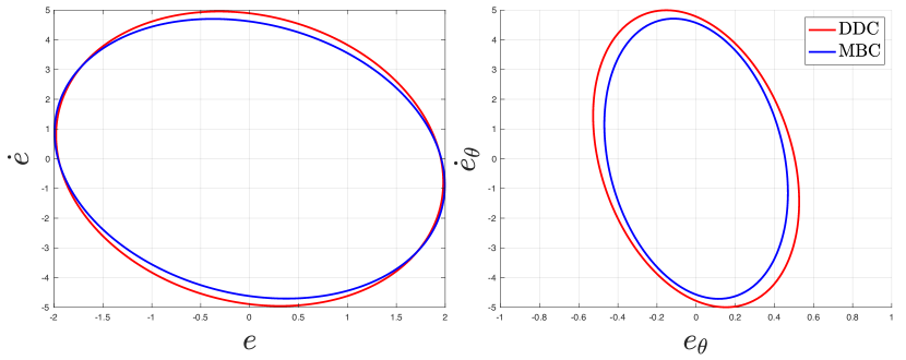
Figure 1: ROAs of NNs trained by DDC and MBC

Under the same settings, the NN trained by our proposed DDC approach shows superior performance in terms of both prediction accuracy and the size of the ROA compared to that trained by MBC approach. One intuitive explanation is that the MBC approach relies on one specific identified model for NFL design, while the DDC approach finds the “best” model for NFL design. Therefore, an end-to-end direct method may outperform indirect methods [16]. We will leave rigorous analysis to our future work.

V-B Existing NN Controller Fine-Tuning

We now consider the same task but in a different scenario to verify the effectiveness of our fine-tuning algorithm. In this case, we assume that there is already a trained controller for the vehicle. As there is no stability guarantee in a traditional NN training algorithm, we want to verify its stability and this is not possible, modify the NN so that we can verify that the new NFL is stable. As we have no access to the training data and hope its structure and other performances remain unchanged, the Algorithm 2 is applied to fine-tune it.

After fine-tuning the NN controller, we simulate the state variation from the same random initial point under input signals of two controllers. The sampling time is $0.02$ s and the result can be shown as following figure.

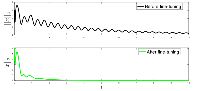
Figure 2: Simulation under the control of existing NN and fine-tuned NN

Here we use $||x||_{2}$ as the value of vertical axis to reflect the variation of the state. Obviously, the NN controller before fine-tuning fails to stabilize the system in a long period, and it is verified as unstable by the data-driven stability verification method [20]. After 5 iterations, the proposed algorithm converges and the fine-tuned controller is guaranteed to result in a stable NFL. The fine-tuning process is more efficient compared to training a new NN controller in terms of the running time. The total time for the former is 0.692 s and the average time for NN training is more than 30 mins. All simulations are performed on a laptop with Apple M2 chip. The MOSEK solver is used to solve the SDP and QP in our problem.

VI Conclusions And Future Works

This paper proposes a data-driven method to design or fine-tune NN controllers for unknown linear systems. The design problem can be formulated as an optimisation problem and then solved by our proposed iterative algorithms using a data-driven approach. Compared to traditional NN controller design methods, one algorithm solves an SDP that includes stability constraints in each iteration. In this way we obtain a controller with stability guarantees. The second algorithm we propose can provide stability guarantee for existing NN controllers by fine-tuning its weights and biases slightly without changing its structure. Compared to retraining a controller for the system, this method significantly improves efficiency. We use a vehicle lateral control example to demonstrate the proposed methods and compare it with model-based approaches. The results demonstrate that even without identifying the system directly, we can design NN controllers for unknown systems based on data. In our example, the controller designed directly even shows better performance in terms of accuracy and stability (in terms of region of attraction) compared to that designed indirectly. In the future we will extend our method to nonlinear Neural Feedback Loops using Sum of Squares methods.

References

- [1] A. G. Barto, R. S. Sutton, and C. W. Anderson, “Neuronlike adaptive elements that can solve difficult learning control problems,” IEEE transactions on systems, man, and cybernetics, no. 5, pp. 834–846, 1983.
- [2] C. W. Anderson, “Learning to control an inverted pendulum with connectionist networks,” in 1988 American Control Conference, 1988, Conference Proceedings, pp. 2294–2298.
- [3] W. Li and J. J. E. Slotine, “Neural network control of unknown nonlinear systems,” in 1989 American Control Conference, 1989, Conference Proceedings, pp. 1136–1141.
- [4] Y. Chen, Y. Shi, and B. Zhang, “Optimal control via neural networks: A convex approach,” arXiv preprint arXiv:1805.11835, 2018.
- [5] F. Fabiani and P. J. Goulart, “Reliably-stabilizing piecewise-affine neural network controllers,” IEEE Transactions on Automatic Control, vol. 68, no. 9, pp. 5201–5215, 2023.
- [6] E. Kaufmann, L. Bauersfeld, A. Loquercio, M. Müller, V. Koltun, and D. Scaramuzza, “Champion-level drone racing using deep reinforcement learning,” Nature, vol. 620, no. 7976, pp. 982–987, 2023.
- [7] S. Gowal, K. D. Dvijotham, R. Stanforth, R. Bunel, C. Qin, J. Uesato, R. Arandjelović, T. Mann, and P. Kohli, “On the effectiveness of interval bound propagation for training verifiably robust models,” arXiv preprint, 2019.
- [8] M. Fazlyab, M. Morari, and G. J. Pappas, “Safety verification and robustness analysis of neural networks via quadratic constraints and semidefinite programming,” IEEE Transactions on Automatic Control, vol. 67, no. 1, pp. 1–15, 2022.
- [9] M. Newton and A. Papachristodoulou, “Neural network verification using polynomial optimisation,” in 2021 60th IEEE Conference on Decision and Control (CDC), 2021, Conference Proceedings, pp. 5092–5097.
- [10] M. Fazlyab, A. Robey, H. Hassani, M. Morari, and G. Pappas, “Efficient and accurate estimation of lipschitz constants for deep neural networks,” Advances in Neural Information Processing Systems, vol. 32, 2019.
- [11] P. Pauli, N. Funcke, D. Gramlich, M. A. Msalmi, and F. Allgöwer, “Neural network training under semidefinite constraints,” in 2022 IEEE 61st Conference on Decision and Control (CDC), 2022, Conference Proceedings, pp. 2731–2736.
- [12] P. Pauli, A. Koch, J. Berberich, P. Kohler, and F. Allgöwer, “Training robust neural networks using lipschitz bounds,” IEEE Control Systems Letters, vol. 6, pp. 121–126, 2022.
- [13] H. Yin, P. Seiler, M. Jin, and M. Arcak, “Imitation learning with stability and safety guarantees,” IEEE Control Systems Letters, vol. 6, pp. 409–414, 2022.
- [14] F. Gu, H. Yin, L. E. Ghaoui, M. Arcak, P. Seiler, and M. Jin, “Recurrent neural network controllers synthesis with stability guarantees for partially observed systems,” Proceedings of the AAAI Conference on Artificial Intelligence, vol. 36, no. 5, pp. 5385–5394, 2022. [Online]. Available: https://ojs.aaai.org/index.php/AAAI/article/view/20476
- [15] N. Junnarkar, H. Yin, F. Gu, M. Arcak, and P. Seiler, “Synthesis of stabilizing recurrent equilibrium network controllers,” in 2022 IEEE 61st Conference on Decision and Control (CDC), 2022, Conference Proceedings, pp. 7449–7454.
- [16] R. Sepulchre, “Data-driven control: Part one of two [about this issue],” IEEE Control Systems Magazine, vol. 43, no. 5, pp. 4–7, 2023.
- [17] C. D. Persis and P. Tesi, “Formulas for data-driven control: Stabilization, optimality, and robustness,” IEEE Transactions on Automatic Control, vol. 65, no. 3, pp. 909–924, 2020.
- [18] M. Guo, C. D. Persis, and P. Tesi, “Data-driven stabilization of nonlinear polynomial systems with noisy data,” IEEE Transactions on Automatic Control, vol. 67, no. 8, pp. 4210–4217, 2022.
- [19] S. Prajna, A. Papachristodoulou, and W. Fen, “Nonlinear control synthesis by sum of squares optimization: a lyapunov-based approach,” in 2004 5th Asian Control Conference (IEEE Cat. No.04EX904), vol. 1, 2004, Conference Proceedings, pp. 157–165 Vol.1.
- [20] H. Wang, Z. Xiong, L. Zhao, and A. Papachristodoulou, “Model-free verification for neural network controlled systems,” arXiv preprint arXiv:2312.08293, 2023.
- [21] S. P. Boyd and L. Vandenberghe, Convex optimization. Cambridge university press, 2004.
- [22] H. Yin, P. Seiler, and M. Arcak, “Stability analysis using quadratic constraints for systems with neural network controllers,” IEEE Transactions on Automatic Control, vol. 67, no. 4, pp. 1980–1987, 2022.