Transformer Models for Quantum Gate Set Tomography

Abstract

Quantum computation represents a promising frontier in the domain of high-performance computing, blending quantum information theory with practical applications to overcome the limitations of classical computation. This study investigates the challenges of manufacturing high-fidelity and scalable quantum processors. Quantum gate set tomography (QGST) is a critical method for characterizing quantum processors and understanding their operational capabilities and limitations. This paper introduces Ml4Qgst as a novel approach to QGST by integrating machine learning techniques, specifically utilizing a transformer neural network model. Adapting the transformer model for QGST addresses the computational complexity of modeling quantum systems. Advanced training strategies, including data grouping and curriculum learning, are employed to enhance model performance, demonstrating significant congruence with ground-truth values. We benchmark this training pipeline on the constructed learning model, to successfully perform QGST for $3$ gates on a $1$ qubit system with over-rotation error and depolarizing noise estimation with comparable accuracy to pyGSTi. This research marks a pioneering step in applying deep neural networks to the complex problem of quantum gate set tomography, showcasing the potential of machine learning to tackle nonlinear tomography challenges in quantum computing.

1 Introduction

Quantum computation is an emerging paradigm of computation that has captured the attention of theoretical physicists and computer scientists, as well as stakeholders in high-performance computing. Quantum algorithms can solve problems in specific complexity classes that are asymptotically intractable in all implementations of classical computation. To demonstrate this acceleration in practice, a topical research avenue is on maturing the quantum computing hardware in terms of high-fidelity (decoherence, error rates of quantum operations) and scalability (number of qubits, connectivity) along with quantum software [1]. Though this research endeavor has proved rather a challenging engineering feat [2, 3, 4], rapid strides were made in the last decade with a plethora of physical technologies capable of demonstrating controllable processing of quantum information.

Constructing a quantum computer requires that the experimental setup meets certain conditions, succinctly summarized as the DiVincenzo criteria [5]. A critical criterion is the characterization of the quantum processor, which helps in understanding the fabrication defects and the computing capabilities of these systems. The characterization is performed by building a model of the noise on the system and the set of quantum operations performed on the quantum information units. The latter typically involves inferring the information-theoretic operation experimentally achieved with respect to a set of target gates in a circuit model quantum computer. Once this operation – termed quantum gate set tomography (QGST) [6] – is performed, the updated experimental model of the quantum gates can be used precisely to determine the required sequence of quantum gates to achieve the transformation for a quantum algorithm.

Tomographic approaches build a detailed model for a system or component in a latent space by fitting that model to the data from numerous independent tests that reveal partial information about the system. The nature of this latent space depends on the representation of the system model. For instance, in medical imaging, by aggregating information from multiple 2D sinograms of CT scans, one can reconstruct a full 2D/3D CT image. Reconstructing a maximally fitting model for the experimental data is computationally expensive. Quantum tomography is particularly expensive as the space of possible observations is continuous and grows exponentially with the system size.

Various machine learning techniques are used to address the computational cost in tomography [7]. However, these techniques have not yet been utilized for quantum gate set tomography. Our contribution presented in this work is three-fold. Firstly, we develop a first-of-its-kind machine-learning model for quantum gate set tomography (Ml4Qgst). To this purpose, we harness the transformer neural network model [8] and tune it for the input-output settings of QGST. Generative models like GAN have been used for quantum state tomography [9]. However, QGST is substantially different due to non-linearity, multi-model regression, and worse computational scaling costs, making it challenging to reuse the models from other quantum tomography tasks. As we show later, QGST can be framed as a language learning task, thus prompting our choice of employing the Transformer model. Secondly, contrary to directly estimating the full process matrices in traditional algorithms, our approach ensures the resulting process matrices are always completely positive and trace preserving (CPTP) and without the necessity to perform gauge fixing. Thus, instead of fully reconstructing the process matrices with no prior knowledge, we are interested in the pragmatic setting of inferring the model drift between the intended theoretical process and the experimentally achieved process. And, thirdly, we incorporate advanced training techniques of data grouping, curriculum learning, and computation of the loss function to increase the performance of our model. Our model predicts error parameters from the error channels and subsequently generates the corresponding estimated process matrices of the gate set.

The rest of the article is organized as follows. In Section 2, the problem setting and required definitions are introduced. We contrast this research with related works on machine learning for quantum tomography. In Section 3, the method and the transformer architecture used in this research are elaborated. Section 4 discusses the advanced training techniques in the experimental settings, while in Section 5, the corresponding results of the experiments are presented. Section 7 concludes the article.

2 Problem setting and definitions

In this section, we present some required background for the article. Firstly, the background theory of gate set tomography based on the super operator formalism is presented. After that, we present how artificial neural networks can be employed for quantum tomography, directing the discussion towards the transformer model that is used in this research.

2.1 Gate set tomography

Different from traditional quantum process tomography, which implicitly assumes known, hence near-zero state preparation and measurement (SPAM) errors, as shown in Figure 1, gate set tomography relaxes this assumption by directly incorporating gates as both preparation and measurement operators or formally as preparation and measurement fiducials. In a quantum computer characterization setting, rather than probing each individual gate using traditional process tomography, gate set tomography aims to simultaneously reconstruct the full gate set using the maximum likelihood method [10]. By measuring the outcomes prescribed by a list of gate sequences that acts to amplify errors on each gate, as shown in the bottom of Figure 1, one can run an optimization algorithm to find out all the parameterized process matrices within the gate set. It is precisely due to this ‘all in one’ tomographic method that gate set tomography has the highest reconstruction accuracy versus traditional state tomography and process tomography, which are largely plagued by the problem of SPAM errors. However, the trade-off of gate set tomography is immediately obvious, in which way more computational resources have to be used to solve for this ‘simultaneous maximum likelihood’ across all gate sequences. This can be understood as maximizing the likelihood function in GST is highly non-convex, in stark contrast to state and process tomography, where each observable probability is a linear function of the parameter [10]. Based on this observation, using deep learning techniques to capture complex non-linear relationships would be a natural choice.

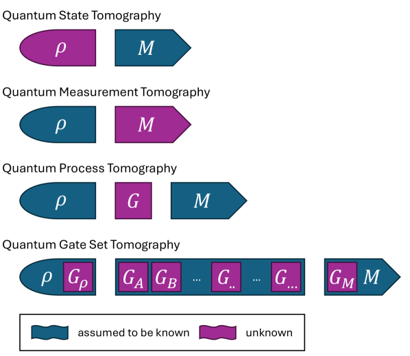
Figure 1: Quantum tomography techniques

2.1.1 Super operator formalism

Similar to the typical Dirac notation in Hilbert space, where a row vector is represented by a bra $\left\langle a\right|$, and column vector by a ket $\left|b\right\rangle$, we denote superbra as $\langle\langle A|$ and superket as $|B\rangle\rangle$. In quantum tomography settings, this conveniently maps a quantum state $\rho$ in the form of a $d\times d$ density matrix in the $d$-dimensional Hilbert space into a complex $d^{2}$-dimensional vector in Hilbert-Schmidt space, with the inner product defined as $\langle\langle A|B\rangle\rangle=\mathit{Tr}(A^{{\dagger}{}}B)$.

In this paper, we use the Pauli Transfer Matrix (PTM) as our super-operator representation, as it is a popular choice in quantum tomography. The PTM basis $\{B_{i}\}$ in Hilbert-Schmidt space has the following properties:

1. Hermiticity: $B_{i}=B_{i}^{{\dagger}}$

2. Orthonormality: $\mathit{Tr}\left(B_{i}B_{j}\right)=\delta_{\mathit{ij}}$

3. Traceless for $i>0$: $B_{0}=I/\sqrt{d}$  and $\mathit{Tr}\left(B_{i}\right)=0,$ for $i>0$

For a single qubit, the normalized PTM basis would be $\{B_{i}\}=\{I/\sqrt{d},\sigma_{x}/\sqrt{2},\sigma_{y}/\sqrt{2},\sigma_{z}/\sqrt{2}\}$. Due to this choice of basis, the PTM vector and super operator are always real.

As an example, we write a single qubit $2\times 2$ density matrix $\rho$ as $|\rho\rangle\rangle$, represented by a real $4\times 1$ column vector, where each coefficient of $|\rho\rangle\rangle$ can be found by taking the inner product $\mathit{Tr}\left(B_{i}^{{\dagger}{}}\rho\right)$.

$$|\rho\text{\textrangle}\text{\textrangle}=\left[\begin{matrix}\mathit{Tr}\left(B_{0}^{{\dagger}{}}\rho\right)\\ \mathit{Tr}\left(B_{1}^{{\dagger}{}}\rho\right)\\ \mathit{Tr}\left(B_{2}^{{\dagger}{}}\rho\right)\\ \mathit{Tr}\left(B_{3}^{{\dagger}{}}\rho\right)\end{matrix}\right]$$

To find the measurement probability of $|\rho\rangle\rangle$ projecting onto the computational basis $\{\left|0\right\rangle,\left|1\right\rangle\}$ we can perform the standard dot product. First, we write the projectors as row vectors,

$$|0\rangle\langle 0|\ \mapsto\langle\langle E_{0}|=\ (1/\sqrt{2},0,\ 0,\ 1/\sqrt{2})$$

$$|1\rangle\langle 1|\ \mapsto\langle\langle E_{1}|=\ (1/\sqrt{2},0,\ 0,\ -1/\sqrt{2})$$

And, then, a standard dot product (or trace) obtains the measurement probabilities $p_{0},p_{1}$ of getting $0$ and $1$,

$$p_{0}=\left\langle\left\langle E_{0}\left|\rho\right.\right\rangle\right\rangle=\mathit{Tr}\left(E_{0}\rho\right)$$

$$p_{1}=\left\langle\left\langle E_{1}\left|\rho\right.\right\rangle\right\rangle=\mathit{Tr}\left(E_{1}\rho\right)$$

Naturally, for any $d^{2}$ quantum state vector, we have the $d^{2}\times d^{2}$ super operator that describes a (noisy) quantum channel, which is not necessarily unitary and/or orthogonal. For any quantum operator $\Lambda$, the PTM satisfies

$$\left\langle\left\langle j\left|R_{\Lambda}\right|k\right\rangle\right\rangle=\mathit{Tr}\left(\sigma_{j}\Lambda\left(\sigma_{k}\right)\right)=\left(R_{\Lambda}\right)_{\mathit{jk}}$$

where, applying a quantum operation/channel $\Lambda$ to a quantum state $|\rho\rangle\rangle$ is represented as left-multiplying a matrix to a vector,

$$|\Lambda(\rho)\rangle\rangle=\ R_{\Lambda}|\rho\rangle\rangle$$

For instance, the PTM of a single qubit rotational gate along the x-axis by $\pi/2$ is given by,

$$R_{X}\left(\pi\text{/}2\right)=\left[\begin{matrix}1&0&0&0\\ 0&1&0&0\\ 0&0&0&-1\\ 0&0&1&0\end{matrix}\right]$$

Corresponding to a quantum operation $\Lambda\left(\rho\right)=U\rho U^{{\dagger}{}}$, $U$ is the unitary single qubit operator.

2.2 Tomography using deep neural networks

The goal of tomography in any general setting is to learn a latent space $z$ that maximally matches with the observed data $x$. The nature of this latent space depends on different scenarios. For instance, referring back to medical imaging, the dimension of $z$ (the reconstructed 2D/3D CT image) is the same or higher than the observed data $x$ (2D sinograms). Notably, both $z$ and $x$ reside in the pixel space that requires little to no transformation when passed to typical neural network models like convolutional neural network (CNN) [11], [12], [13] or diffusion model [14], [15], [16].

Quantum tomography is strikingly different as the $z$ and $x$ do not reside in the same space. For quantum state(process) tomography, the latent space $z$ is the density(process) matrix that takes the form of a square matrix, whereas the observed data $x$ refers to the measured counts or normalized probabilities from the quantum device, conditioned on a certain measurement and/or preparation operators.

The same mismatch between latent space and observed space persists in gate set tomography, which prevents the direct implementation of typical deep generative models from image processing [9]. Instead, an intermediate function has to be used in order to map the latent space to the observed space, namely, an analytical function that maps the neural network output to the expected probabilities under supervised learning.

The advancement of neural network models and computer hardware in the last decade have brought forth numerous novel applications in the industry, such as autonomous robotics via reinforcement learning [17], image generation [18] via diffusion model, text generation via large language model [19] and so much more. Riding on this trend, the quantum physics community has borrowed these techniques from the industry for quantum tomography. Earlier work mainly focuses on using restricted Boltzmann machines for simple quantum state tomography tasks that can be represented by pure states. Later works employ deep neural networks for more difficult tasks such as general density matrix reconstruction [9] and process matrix construction [20] . The methods being used range from simple feed-forward networks to more advanced models such as conditional generative adversarial networks and transformer models. For instance, GAN demonstrated good convergence behavior in [9] when reconstructing a density matrix in the quantum state tomography setting, but this is only because the QST problem is linear in nature. It has been shown that GAN is susceptible to mode collapse [21], which is particularly troubling when the data being trained on are multi-modal. In GST, the problem that has to be solved is highly non-linear, with multi-modal data corresponding to multiple different gates that have to be estimated, as well as the underlying error parameters that represent those gates.

3 Ml4Qgst model

Contrary to most existing publications that directly use deep neural networks to reconstruct the full density or process matrix in quantum state or process tomography settings, we aim to predict physical error parameters in gate set tomography instead and then use analytical functions to reconstruct the full process matrices afterward, as a way to ensure that the completely positive and trace preserving (CPTP) condition is met and remove the necessity of gauge fixing.

Furthermore, we alleviate the shortcomings of GANs by proposing a transformer model-based deep neural network, which excels in encoding and processing sequences [8], compared to standard convolution-based methods that are fundamentally limited by kernel sizes. In addition, promising results have already been shown in quantum state tomography setting recently using transformer-based techniques [22], [23].

3.1 Transformer model

Since the invention of the transformer architecture [8], the world has been revolutionized by the success and capabilities that GPT-4 [24] and other large language models (LLM) provide. Here we briefly explain what a transformer is, specifically the encoder block that we will use in this paper.

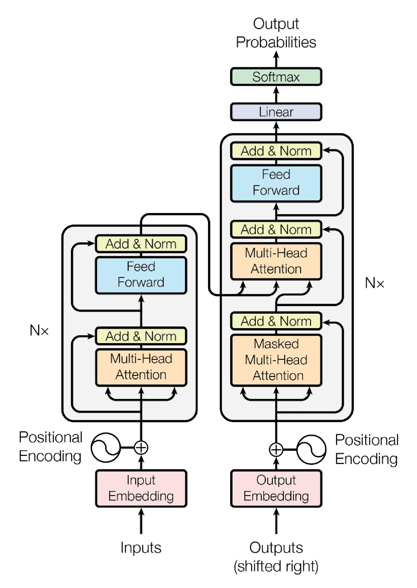
Figure 2: The Transformer model architecture with its encoder block (left) and decoder block (right) [8].

Figure 2 shows the complete transformer architecture that is used for text generation in the original implementation, and it can be further divided into an encoder (left) and a decoder block (left). Within each block, the main component that empowers the transformer is the multi-head attention layer (see orange-colored rectangle). As its name implies, the attention layer’s goal is to ‘pay attention’ to the sequences, elements, or structures of the input data, similar to what humans do. Mathematically, this is done by constructing arrays (query, key, value) and performing a dot product between query and key to obtain an attention score matrix. Afterward, a softmax operation is applied to the attention score matrix to obtain a new matrix corresponding to attention weights(probabilities). Finally, this attention weight matrix is multiplied with value, yielding a new weighted value output. The attention mechanism is most commonly seen in LLMs to process sequences of input text or, alternatively, focus on the underlying structure of images in computer vision [25].

In our paper, we only make use of the encoder block to encode input data and subsequently use a simple feed-forward network for regression. We skip the transformer decoder commonly used in natural language processing, as our goal is not to generate new sequences but to predict error parameters. This model encodes the gate sequence data naturally, similar to text encoding which has been widely adopted in the industry. We make use of self/cross attention mechanisms, which aim to focus on the information (process matrix) of each individual gate and the inter-relationship between gate sequences and normalized probabilities, respectively. By aggregating all the information through the transformer pipeline, we estimate the error parameters from the gate set tomography experiment.

The remainder of the section describes the main components of our Ml4Qgst implementation. Its components consist of 1) separate embedding layers for both integer-encoded gate sequences and normalized probabilities, 2) separate positional encoding for both gate sequences and normalized probabilities, 3) cross attention layer to aggregate information from two branches, 4) transformer block to encode the aggregated information, 5) fully connected layer to output physical error parameters. A schematic of the neural network architecture is shown in Figure 3.

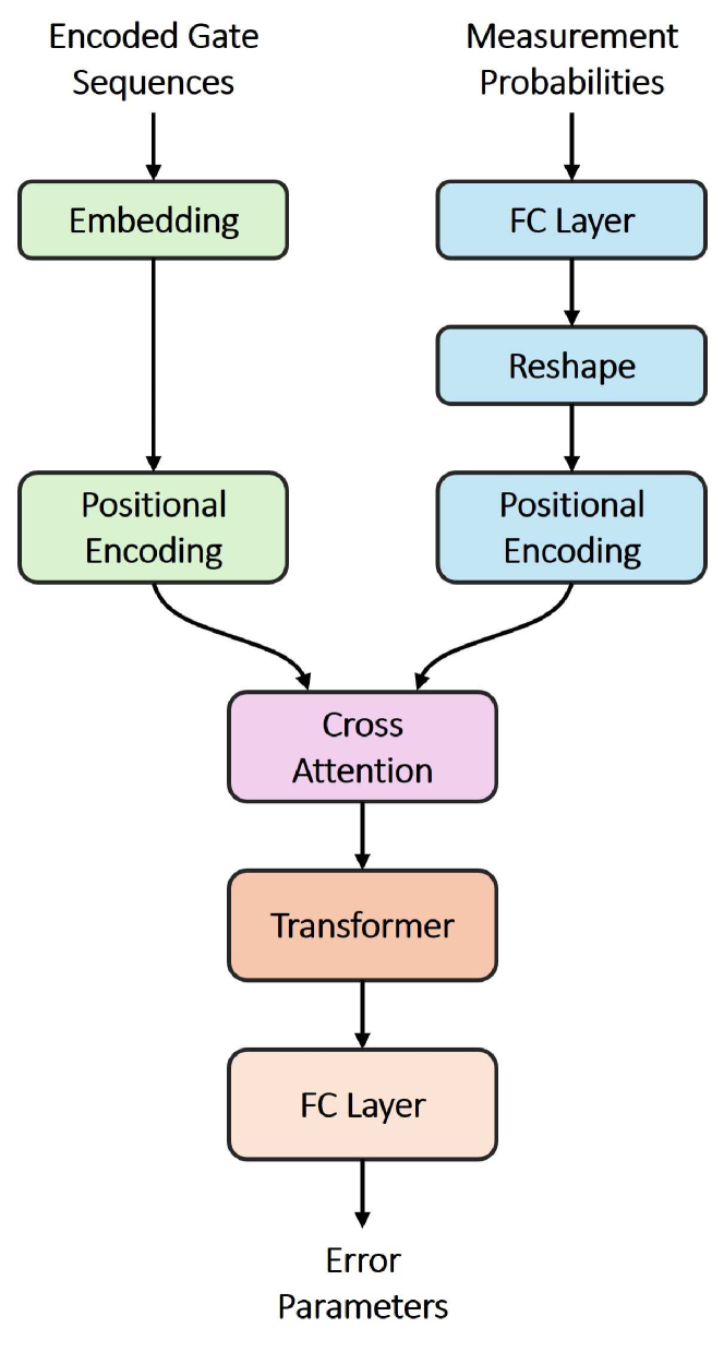
Figure 3: A schematic overview of Ml4Qgst, our transformed-based neural network architecture for GST.

3.2 Embedding gate sequences and normalized probabilities

In gate set tomography, each gate sequence output measures counts for each computational basis and can be converted into normalized probabilities for each basis state. By aggregating the information of multiple pairs of gate sequences and normalized probabilities, one can extract the information of the process matrix of each gate used. The gate sequences are first preprocessed by integer encoding and zero padding, where each gate is mapped to a unique integer, and the gate sequences are zero-padded to match the longest gate sequence in the dataset. The encoded gate sequences are then passed to an embedding layer used in a typical transformer setting. Besides that, the normalized probabilities are passed to a fully connected layer and are subsequently reshaped to emulate the effect of an embedding layer.

This way, both branches will have an extra learnable feature dimension that is ready to be processed by a transformer block later on.

3.3 Positional encoding

We use the standard sine and cosine positional encoding for both embedded gate sequences and normalized probabilities, that are flattened beforehand. As each individual pair of gate sequence and normalized probabilities yields little tomographic information, we instead group multiple pairs together to increase the receptive field. Positional encoding is then applied element-wise to this flattened embedded gate sequence and normalized probabilities at each branch.

3.4 Cross attention layer

After embedding and positional encoding at each branch, a cross-attention layer is used to process the relationship between the grouped gate sequences and normalized probabilities. We choose cross-attention instead of simple concatenation to avoid the vast data shape mismatch between gate sequences and normalized probabilities that can possibly drown out the training signal.

3.5 Transformer encoder block

A standard multi-layer transformer encoder block is used to process the aggregated information. It includes typical components such as a multi-head attention layer, add & norm layer, and feed-forward layer.

3.6 Fully connected layers

Finally, fully connected layers are used for regression after the transformer block, outputting predicted physical error parameters.

4 Experiments

We evaluate Ml4Qgst using the open-source Python package pyGSTi [26], with the capability of: 1) customizing the process matrix of each individual gate within a gate set, 2) selecting appropriate fiducials for the customized gate set, 3) generating appropriate gate sequences for the GST experiment, 4) simulating measured counts for the gate sequences.

4.1 pyGSTi simulation settings

The pyGSTi Python package uses Pauli Transfer Matrices (PTM) as the default process matrix throughout the GST implementation. Here we replaced the built-in single qubit XYI model with our custom PTM, specifically the X and Y rotational gates. These custom gates are parametrized with physical error parameters and in our case, the over-rotational angles and depolarizing errors. We then use the custom X and Y rotational gates, together with the built-in function, to find suitable fiducials, that is, a handful of short gate sequences that are used repeatedly and combinatorially to generate GST experiments. After that, we run the built-in single qubit XYI GST experiment function to generate gate sequences and simulated measured counts. The number of shots is set to $10,000$, and the maximum sequence length to $2^{5}$, and the sampling error to binomial. Figure 4 shows the overall data pipeline from input to loss computation.

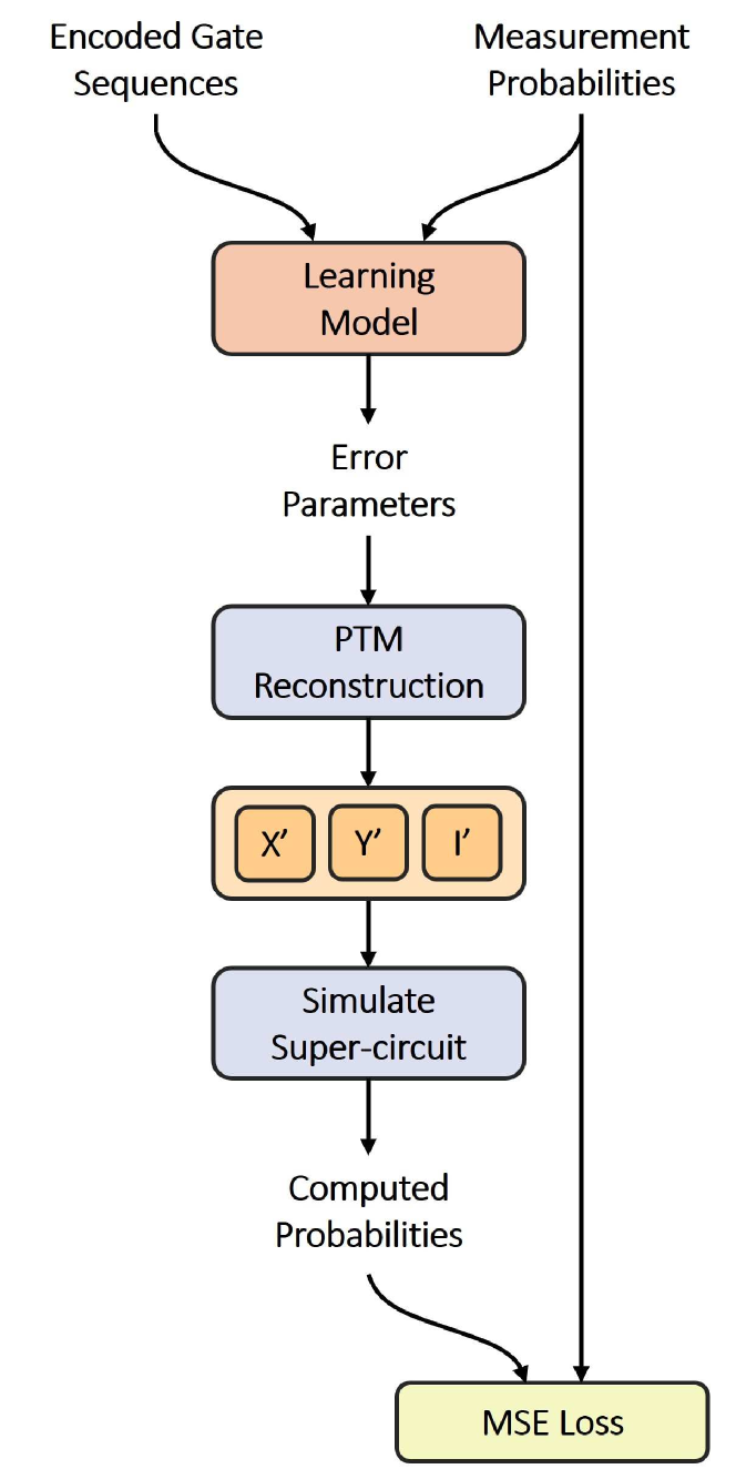
Figure 4: Overall data pipeline of Ml4Qgst from input to output and MSE loss computation.

4.2 Training details

4.2.1 Data grouping

As mentioned briefly in 3.2, the gate sequences generated by pyGSTi are converted from strings to unique integers and, subsequently, zero-padded to match the maximum length of a sequence in the dataset, whereas simulated measured counts are normalized into probabilities. After that, both gate sequences and probabilities datasets are divided into groups, specified by a hyperparameter ‘group_size’. In order to ensure all groups have the same number of elements, we choose to repeat the elements inside the last group instead of zero padding to preserve overall data quality.

4.2.2 Curriculum learning

Drawing inspiration from the way humans learn, curriculum learning aims to achieve better performance and faster convergence by starting with simpler or more fundamental examples and progressively introducing more complex ones [27], we conveniently call it stage training here, starting from easier to more difficult stages. In the following, We make use of curriculum learning to further divide the whole dataset into parts, again specified by a hyperparameter ‘part_size’. The dataset is sorted in ascending order based on the non-zero length of the gate sequences. This ensures that the model learns global features from shorter gate sequences in the beginning and then progressively fine-tunes predictions in later stages when it sees longer gate sequences. This learning methodology is similar to the algorithm implemented in the GST paper [10], in which the authors iteratively add longer sequences, including the previously seen sequences in an accumulative way during optimization. We instead opt for a non-accumulative approach as in standard curriculum learning, and saving computational resources required.

4.2.3 Analytical PTM reconstruction

Based on the predicted physical error parameters, namely the over-rotational angles and depolarizing errors, we analytically reconstruct PTMs corresponding to the gates within the gate set.

4.2.4 Computing loss

As each grouped data outputs one set of physical error parameters prediction, it also has its own set of reconstructed PTMs. We compute probabilities analytically for all the gate sequences within a group, using the same set of reconstructed PTMs. This procedure is performed iteratively group by group within a particular stage set by curriculum learning. Finally, we compute the mean squared error loss between the ground-truth probabilities and the reconstructed probabilities.

5 Results

In the following, we will explain the choice of loss function in our experiment, analyze convergence behavior during neural network training and compare benchmarking results from different commonly used metrics.

5.1 Choice of loss function

The GST paper [10] uses two loss functions for long-sequence GST optimization, the multinomial log-likelihood function $log\left(L\right)$ for a $m_{s}$ outcomes Bernoulli scheme, and the $\chi^{2}$ estimator.

$$log\left(L\right)=\sum_{s}\ log\left(L_{s}\right)=\sum_{s,\beta_{s}}\ N_{s}f_{s,\beta_{s}}log\left(p_{s,\beta_{s}}\right)$$

$$\chi^{2}=\sum_{s,\beta_{s}}\frac{N_{s}\left(p_{s,\beta_{s}}-f_{s,\beta_{s}}\right)^{2}}{p_{s,\beta_{s}}}$$

where $s$ denotes the index of a circuit, and let $m_{s}$ be the number of outcomes of $s$, $N_{s}$ the total number of times circuit $s$ was repeated, $N_{s,\beta_{s}}$ the number of times outcome $\beta_{s}$ was observed, $p_{s,\beta_{s}}$ the probability predicted by the model of getting outcome $\beta_{s}$ from circuit $s$, and $f_{s,\beta_{s}}=N_{s,\beta_{s}}/N_{s}$ is the corresponding observed frequency.
The authors used the $\chi^{2}$ estimator as a proxy of $log(L)$ during optimization except for the last phase, as it is more computationally efficient. Then, $log(L)$ is used in the final phase to steer the estimate to comply with the true statistical derivation. Here, we further simplify the $\chi^{2}$ estimator to mean-squared error (MSE) loss, which has also been used in simpler linear GST settings. Alternatively, MSE loss can be seen from the perspective of reducing the likelihood function to a normal distribution by invoking the central limit theorem [28].

$$\mathit{loss}=\sum_{s,\beta_{s}}\frac{\left(p_{s,\beta_{s}}-f_{s,\beta_{s}}\right)^{2}}{\sigma_{s,\beta_{s}}^{2}}$$

where $\sigma_{s,\beta_{s}}^{2}$ = $p_{s,\beta_{s}}(1-p_{s,\beta_{s}})/N_{s}$ is the sampling variance in the measurement.

5.2 Convergence analysis

In the following, we will explain the training trajectories of predicted error parameters by delving a little bit deeper into the technical implementation.

Figures 5, 6 show the convergence behavior plots for depolarizing error and Figures 7, 8 for over rotational angle. Both types of plots contain the X-gate and Y-gate training trajectories, the x-axis always represents the number of training epochs and the y-axis indicates the depolarization amplitude and over rotational angle in radian respectively. For both, the predicted depolarizing errors and the over-rotational angles, the predicted values exhibit oscillatory behavior at the beginning of each stage of curriculum learning, where an entirely new set of data was fed into the neural network for further training. This is indicated at epochs 90, 190, and 263, corresponding to the start of stages 2, 3, and 4.

Because we use the tanh activation function at the neural network output layer and subsequently take absolute values in the custom training loop, the plots for depolarizing errors shown below will generally have the predicted values jumping between positive and negative. This is intended, as we want the predicted depolarizing error values to be close to and centered at zero, where the tanh activation function is the prime candidate.

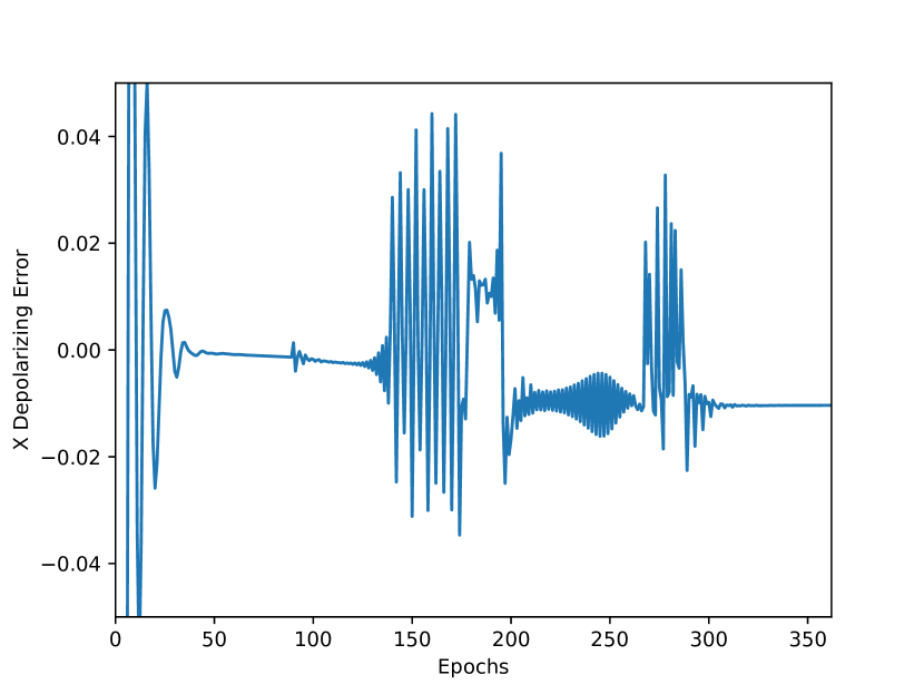
Figure 5: Training trajectory of the predicted X-gate depolarizing error with curriculum learning, tanh activation function is used at the final output layer to allow large gradient near zero, a subsequent absolute value function is added to ensure predicted value is between 0 and 1.

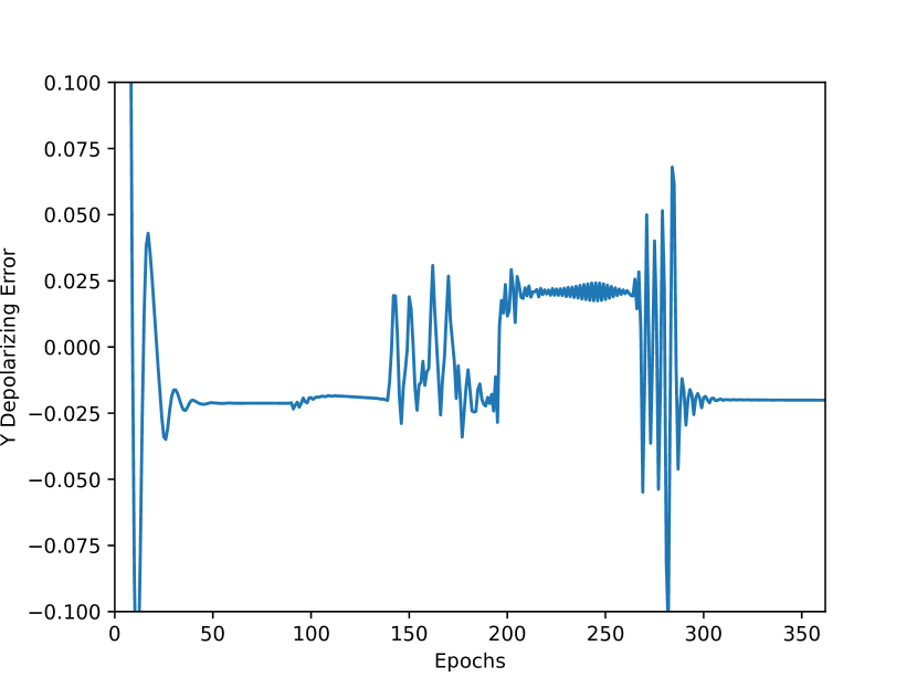
Figure 6: Training trajectory of the predicted Y-gate depolarizing error with curriculum learning, tanh activation function is used at the final output layer to allow large gradient near zero, a subsequent absolute value function is added to ensure predicted value is between 0 and 1.

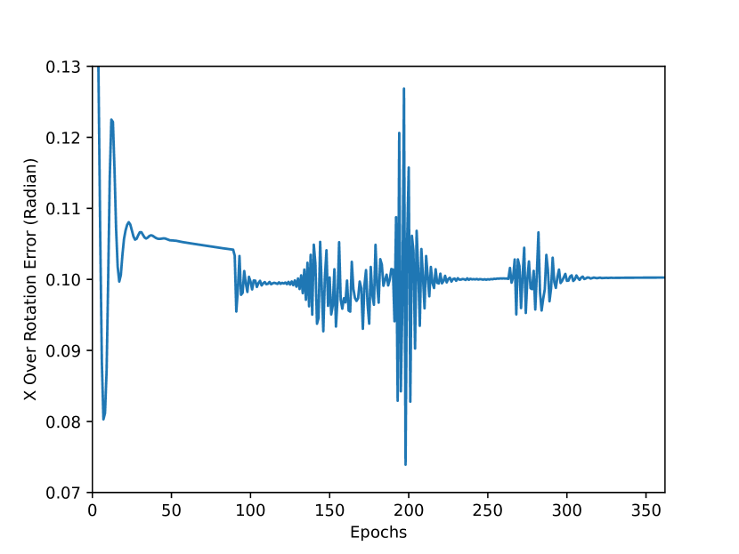
Figure 7: Training trajectory of the predicted X-gate over-rotational error with curriculum learning, tanh activation function is used at the final output layer to ensure the output value is between -1 and +1 (radian).

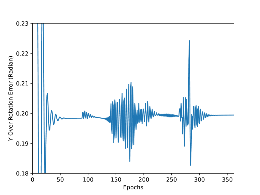
Figure 8: Training trajectory of the predicted Y-gate over-rotational error with curriculum learning, tanh activation function is used at the final output layer to ensure the output value is between -1 and +1 (radian).

Additionally, we showed that without curriculum learning, the model fails to converge within the normalized number of epochs, which is equal to the number of epochs for each stage in the curriculum learning. Figures 9, 10, 11, 12 show the convergence trajectories without curriculum learning. The empirical evidence here shows that curriculum learning, like the iterative optimization approach from the GST paper, is indeed required for proper convergence.

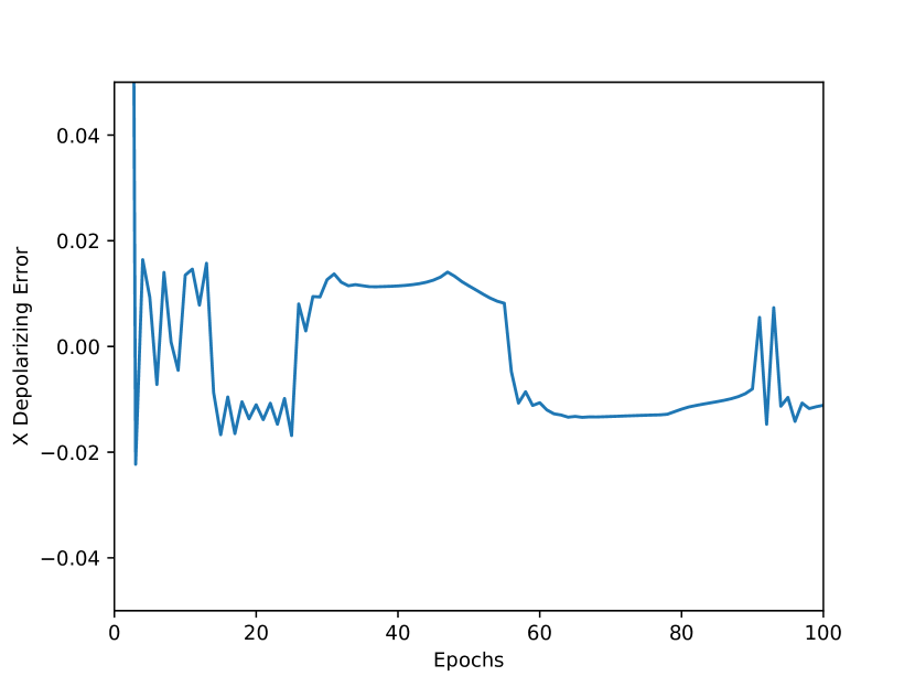
Figure 9: Training trajectory of the predicted X-gate depolarizing error without curriculum learning, tanh activation function is used at the final output layer to allow large gradient near zero, a subsequent absolute value function is added to ensure predicted value is between 0 and 1.

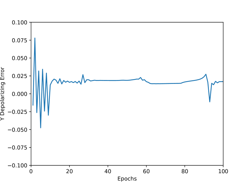
Figure 10: Training trajectory of the predicted Y-gate depolarizing error without curriculum learning, tanh activation function is used at the final output layer to allow large gradient near zero, a subsequent absolute value function is added to ensure predicted values is between 0 and 1.

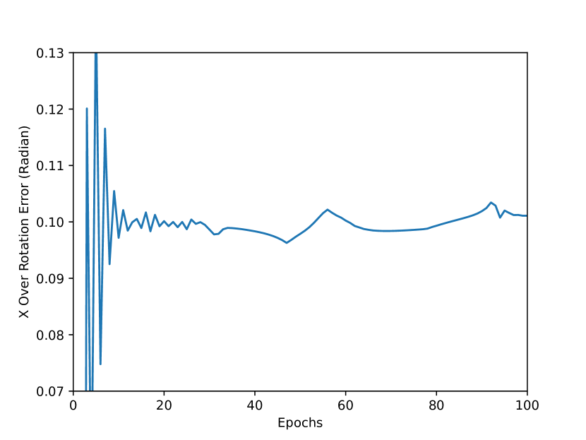
Figure 11: Training trajectory of the predicted X-gate over-rotational error without curriculum learning, tanh activation function is used at the final output layer to ensure the output value is between -1 and +1 (radian).

Figure 12: Training trajectory of the predicted Y-gate over-rotational error without curriculum learning, tanh activation function is used at the final output layer to ensure the output value is between -1 and +1 (radian).

Loss function	With CL	Without CL	Ground-Truth	% Error Ratio (W.O CL/ CL)
MSE (Training)	1.9668e-05 (-0.08%)	2.1339e-05 (-8.41%)	1.9683e-05 (0%)	105.1
KL divergence	5.2119e-05 (-2.35%)	5.6215e-05 (-10.39%)	5.0923e-05 (0%)	4.4
$\chi^{2}$ estimator	0.003118 (-2.06%)	0.003380 (-10.64%)	0.003055 (0%)	5.2
-$log\left(L\right)$	16.11541 (-1.86e-5%)	16.11554 (-9.93e-4%)	16.11538 (0%)	53.4

Table 1: Benchmarking for different loss functions: MSE, KL divergence, $\chi^{2}$ estimator, -log $L$, with and without curriculum learning.

5.3 Benchmarking

To show that our predicted values are in good agreement with the ground-truth values from the simulation, we choose KL-divergence, $\chi^{2}$ estimator, and full $log\left(L\right)$ function as a benchmark. We compare the benchmark results among three cases: ground-truth values, predicted values with curriculum learning (CL), and predicted values without curriculum learning, as shown in Table 1. The zero reference point for percentage error is set to ground truth in the table.

We first look at MSE, KL divergence, and $\chi^{2}$ estimator, which all are the functions that measure the distance between probability distributions. It is no surprise that MSE has the lowest percentage error, as it was used as the loss function during training. We can also see a consistent trend among the three benchmarks, where the results without CL are much worse than the ones with CL, verifying the necessity of CL during training. Besides looking at just the percentage error, the error ratio between the known bad (without CL) and good (with CL) fit can roughly tell us how large the training signal would be, whereas a bigger ratio usually refers to a larger training signal. It can be seen that MSE and $-log\left(L\right)$ functions have large error ratios, meanwhile KL divergence and $\chi^{2}$ estimator yield small ratios, suggesting MSE and $-log\left(L\right)$ functions are more versatile for training purpose.

Figure 13: (a,b) X and Y gate PTM distance heatmaps between the ground-truth quantum computer (QC) and the Ideal operations, (c,d) X and Y gate PTM distance heatmaps between the ground-truth quantum computer (QC) and the Ml4Qgst predicted operations

Finally, we show the process matrix distance heatmaps in Figure 13, as a standard practice to visualize the estimated results, commonly used in quantum tomography. To show that the model is indeed estimating the error parameters/ process matrices sensibly, the PTM distance heatmaps between (QC - Ideal) and (Ml4Qgst - QC) are compared, where ideal refers to operations with no depolarizing error and over rotation, QC means ground-truth quantum computer (QC) operations and Ml4Qgst refers to our model predicted operations. Figure 13(a,b) tells us how bad the quantum computer behaves with respect to the ideal operations that we actually want, while Figure 13 (c,d) informs us how well our Ml4Qgst model estimates the ground-truth quantum computer operations. Comparing the X and Y gate distance heatmaps in Figure 13 (c,d), we can roughly see the over-rotation angle and depolarizing error estimation slightly overshoot, with the exception of Y gate undershooting the estimation of over-rotation angle. The percentage differences between the ground truth and the estimated values are 3.6558%(0.5321%) for X(Y) depolarizing error and 0.2615%(-0.2850%) for X(Y) over-rotational angle. This is largely comparable to pyGSTi’s long gate sequence GST results: -0.0341%(0.2670%) and 0.5659%(-0.3705%).

6 Outlook

In this article, we have demonstrated our model is able to produce comparable accuracy with pyGSTi’s implementation. In this section, we explore future improvements for Ml4Qgst, focusing on: 1) bootstrapping, 2) scalability for multi-qubit systems, and 3) zero-shot to few-shot learning.

The most immediate and universal use case for a trained deep neural network model would be bootstrapping existing tomographic approaches, where an end user queries the trained model to obtain a list of fairly accurate predictions and subsequently uses this as an initial guess input to another mathematically rigorous traditional analytical or numerical model, vastly reduces the computation resource and time required from traditional approaches, while still retaining the superior prediction accuracy, compared to using deep neural network alone.

The next use case would be scaling up gate set tomography to multi-qubit systems. Although not demonstrated in this proof-of-concept paper, the transformer has been proven for capturing long-range relationships in natural language processing, which, in turn, should work well when processing multi-qubit long sequence quantum circuits. To draw a parallel, in terms of encoding quantum circuits for specific use cases, the transformer will be a natural extension and improvement to existing CNN-based quantum circuit optimization [29]. In essence, we welcome future research in the quantum community to make use of transformer models to process quantum circuit-related applications.

Finally, our Ml4Qgst model can potentially benefit from zero to few-shot learning. That is, focusing on a fixed set of quantum circuits that were used in training, the model can predict new error parameters if the end user provide a new set of probabilities corresponding to those quantum circuits, with no to little further training required. Namely, we can treat probabilities as conditioning information to alter model output accordingly, similar to text-prompted image generation. This can be done with minor architectural change to Ml4Qgst, where the conditional information (probabilities) is injected directly to each transformer block via multi-head cross attention mechanism or the more advanced adaLN-zero modulation [30], instead of a single pass multi-head cross attention before the transformer blocks as in the current model.

7 Conclusion

In this article, we presented a transformer-based neural network model for quantum gate set tomography. By leveraging self- and cross-attention mechanisms to aggregate information from the measured GST data, we subsequently pass the processed data into a feed-forward neural network to obtain the estimated error parameters. In combination with curriculum learning, the model converges in a stable way, and the final estimated results are in good agreement with ground-truth values. Our results are a proof of concept that demonstrates that deep neural network models can also be used in tackling difficult highly non-linear tomography problems like gate set tomography. We wish to further improve the efficiency and accuracy of the model for gate set tomography in the future by exploring different neural network architectures and via model fine-tuning. In particular, we believe that leveraging the success of first compressing data in latent space via an auto-encoder that was recently used in diffusion model [18] would greatly reduce the computational footprint for GST. GST can be understood as mapping a large set of measurement data into a small subset of error parameters, where the idea of latent space would naturally come into the picture.

Software Availability

The software developed for this project is available at: https://github.com/QML-Group/ML4GST.

The GST data is generated via the pyGSTi software: https://github.com/sandialabs/pyGSTi.

References

- \bibcommenthead
- Sarkar [2024] Sarkar, A.: Automated quantum software engineering. Automated Software Engineering 31(1), 1–17 (2024)
- Preskill [2018] Preskill, J.: Quantum computing in the NISQ era and beyond. Quantum 2, 79 (2018)
- Leymann and Barzen [2020] Leymann, F., Barzen, J.: The bitter truth about gate-based quantum algorithms in the nisq era. Quantum Science and Technology 5(4), 044007 (2020)
- Ezratty [2023] Ezratty, O.: Where are we heading with nisq? arXiv preprint arXiv:2305.09518 (2023)
- DiVincenzo [2000] DiVincenzo, D.P.: The physical implementation of quantum computation. Fortschritte der Physik: Progress of Physics 48(9-11), 771–783 (2000)
- Greenbaum [2015] Greenbaum, D.: Introduction to quantum gate set tomography. arXiv preprint arXiv:1509.02921 (2015)
- Wang et al. [2019] Wang, G., Zhang, Y., Ye, X., Mou, X.: Machine Learning for Tomographic Imaging. IOP Publishing, ??? (2019)
- Vaswani et al. [2017] Vaswani, A., Shazeer, N., Parmar, N., Uszkoreit, J., Jones, L., Gomez, A.N., Kaiser, Ł., Polosukhin, I.: Attention is all you need. Advances in neural information processing systems 30 (2017)
- Ahmed et al. [2021] Ahmed, S., Muñoz, C.S., Nori, F., Kockum, A.F.: Quantum state tomography with conditional generative adversarial networks. Physical review letters 127(14), 140502 (2021)
- Nielsen et al. [2021] Nielsen, E., Gamble, J.K., Rudinger, K., Scholten, T., Young, K., Blume-Kohout, R.: Gate set tomography. Quantum 5, 557 (2021)
- Gupta et al. [2018] Gupta, H., Jin, K.H., Nguyen, H.Q., McCann, M.T., Unser, M.: Cnn-based projected gradient descent for consistent ct image reconstruction. IEEE transactions on medical imaging 37(6), 1440–1453 (2018)
- Clark and Badea [2019] Clark, D., Badea, C.: Convolutional regularization methods for 4d, x-ray ct reconstruction. In: Medical Imaging 2019: Physics of Medical Imaging, vol. 10948, pp. 574–585 (2019). SPIE
- Kang et al. [2017] Kang, E., Min, J., Ye, J.C.: A deep convolutional neural network using directional wavelets for low-dose x-ray ct reconstruction. Medical physics 44(10), 360–375 (2017)
- Huang et al. [2022] Huang, B., Zhang, L., Lu, S., Lin, B., Wu, W., Liu, Q.: One sample diffusion model in projection domain for low-dose ct imaging. arXiv preprint arXiv:2212.03630 (2022)
- Xia et al. [2023] Xia, W., Niu, C., Cong, W., Wang, G.: Sub-volume-based denoising diffusion probabilistic model for cone-beam ct reconstruction from incomplete data. arXiv e-prints, 2303 (2023)
- Xia et al. [2022] Xia, W., Lyu, Q., Wang, G.: Low-dose ct using denoising diffusion probabilistic model for 20 speedup. arXiv preprint arXiv:2209.15136 (2022)
- Gu et al. [2017] Gu, S., Holly, E., Lillicrap, T., Levine, S.: Deep reinforcement learning for robotic manipulation with asynchronous off-policy updates. In: 2017 IEEE International Conference on Robotics and Automation (ICRA), pp. 3389–3396 (2017). IEEE
- Rombach et al. [2021] Rombach, R., Blattmann, A., Lorenz, D., Esser, P., Ommer, B.: High-resolution image synthesis with latent diffusion models. 2022 ieee. In: CVF Conference on Computer Vision and Pattern Recognition (CVPR), pp. 10674–10685 (2021)
- Brown et al. [2020] Brown, T., Mann, B., Ryder, N., Subbiah, M., Kaplan, J.D., Dhariwal, P., Neelakantan, A., Shyam, P., Sastry, G., Askell, A., et al.: Language models are few-shot learners. Advances in neural information processing systems 33, 1877–1901 (2020)
- Ahmed et al. [2023] Ahmed, S., Quijandría, F., Kockum, A.F.: Gradient-descent quantum process tomography by learning kraus operators. Physical Review Letters 130(15), 150402 (2023)
- Lala et al. [2018] Lala, S., Shady, M., Belyaeva, A., Liu, M.: Evaluation of mode collapse in generative adversarial networks. High performance extreme computing (2018)
- Cha et al. [2021] Cha, P., Ginsparg, P., Wu, F., Carrasquilla, J., McMahon, P.L., Kim, E.-A.: Attention-based quantum tomography. Machine Learning: Science and Technology 3(1), 01–01 (2021)
- Ma et al. [2023] Ma, H., Sun, Z., Dong, D., Chen, C., Rabitz, H.: Tomography of quantum states from structured measurements via quantum-aware transformer. Technical report (2023)
- Achiam et al. [2023] Achiam, J., Adler, S., Agarwal, S., Ahmad, L., Akkaya, I., Aleman, F.L., Almeida, D., Altenschmidt, J., Altman, S., Anadkat, S., et al.: Gpt-4 technical report. arXiv preprint arXiv:2303.08774 (2023)
- Dosovitskiy et al. [2020] Dosovitskiy, A., Beyer, L., Kolesnikov, A., Weissenborn, D., Zhai, X., Unterthiner, T., Dehghani, M., Minderer, M., Heigold, G., Gelly, S., et al.: An image is worth 16x16 words: Transformers for image recognition at scale. arXiv preprint arXiv:2010.11929 (2020)
- Nielsen et al. [2020] Nielsen, E., Rudinger, K., Proctor, T., Russo, A., Young, K., Blume-Kohout, R.: Probing quantum processor performance with pygsti. Quantum science and Technology 5(4), 044002 (2020)
- Bengio et al. [2009] Bengio, Y., Louradour, J., Collobert, R., Weston, J.: Curriculum learning. In: Proceedings of the 26th Annual International Conference on Machine Learning, pp. 41–48 (2009)
- Greenbaum [2015] Greenbaum, D.: Introduction to quantum gate set tomography. arXiv preprint arXiv:1509.02921 (2015)
- Fösel et al. [2021] Fösel, T., Niu, M.Y., Marquardt, F., Li, L.: Quantum circuit optimization with deep reinforcement learning. arXiv preprint arXiv:2103.07585 (2021)
- Peebles and Xie [2023] Peebles, W., Xie, S.: Scalable diffusion models with transformers. In: Proceedings of the IEEE/CVF International Conference on Computer Vision, pp. 4195–4205 (2023)