Computational issues in Optimization for Deep networks

Abstract

The paper aims to investigate relevant computational issues of deep neural network architectures with an eye to the interaction between the optimization algorithm and the classification performance. In particular, we aim to analyze the behaviour of state-of-the-art optimization algorithms in relationship to their hyperparameters setting in order to detect robustness with respect to the choice of a certain starting point in ending on different local solutions. We conduct extensive computational experiments using nine open-source optimization algorithms to train deep Convolutional Neural Network architectures on an image multi-class classification task. Precisely, we consider several architectures by changing the number of layers and neurons per layer, in order to evaluate the impact of different width and depth structures on the computational optimization performance.

1 Introduction

One of the key areas of artificial intelligence is supervised machine learning (ML), which involves the development of algorithms and models capable of learning a model on a given set of samples and making predictions or decisions based on previously unseen data. In ML community this property is commonly known as generalization capability. In most real-world applications, as well as in the case analyzed in this paper, the system is a neural network trained by minimizing a differentiable loss function measuring the dissimilarity between some target values and the values returned by the network itself. The training process consists in the minimization of a loss function with respect to the network weights and biases, which can result in a complex and large-scale optimization problem.

The crucial role played by optimization algorithms in machine learning, acknowledged since the birth of this research field, has been widely and deeply discussed in the literature, both from an operations research and a computer science perspective. Training a supervised ML model involves, indeed, addressing the optimization problem (Gambella et al (2021)) of minimizing a function, which measures the dissimilarity between predicted and correct values. Simple examples are the different type of regression (Lewis-Beck and Lewis-Beck (2015); LaValley (2008); Ranstam and Cook (2018)), the neural network optimization (Goodfellow et al (2014)), the decision trees (Carrizosa et al (2021); Rokach and Maimon (2010); Bertsimas and Dunn (2017); Buntine (2020)), support vector machines ( Steinwart and Christmann (2008); Tatsumi and Tanino (2014); Suthaharan and Suthaharan (2016); Pisner and Schnyer (2020)). While the underlying idea of stochastic gradient-like methods, proposed by Robbins and Monro (1951), dates back to the 1950s, the research community has deeply investigated its theoretical and computational properties and a vast amount of new algorithms have been developed in the past decades.

Despite all the studies that have already been carried out in this field, which will discuss further, to the best of our knowledge, only a few have tried to answer some relevant computational questions encountered when using optimization methods to train deep neural networks (DNNs). In this paper, we point out and address the following issues in solving training optimization problems to assess the influence of optimization algorithm settings and architectural choices on generalization performances.

• Convergence to local versus global minimizers and the effect of the quality (in terms of training loss) of the solution on the generalization performances;

• effect of the non-monotone behaviour of mini-batch methods with respect to traditional batch methods (L-BFGS) on the computational performances;

• different role of the starting point and regions of attraction on L-BFGS than on mini-batch algorithms;

• importance of the optimization algorithm’s hyperparameters tuning on the optimization and the generalization performances;

• the robustness of hyperparameters setting tuned on a specific architecture and dataset by modifying the number of layers and neurons and the datasets

In this paper, we discuss and try to answer some questions regarding the aforementioned issues. We conduct extensive computational experiments to enforce our main claims:

• generalization performances can be influenced by the solution found in the training process. Local minima can be very different from each other and result in very different test performances;

• traditional batch methods, like L-BFGS, are less efficient and also more sensitive to the starting point than mini-batch online algorithms;

• hyperparameters tuned on a specific baseline problem, namely a given baseline architecture trained on an instance of a class of problems, can achieve better generalization performance than the default ones even on different problems, changing either the architecture and/or the instance in the given class.

To the aim above, we consider the task of training convolutional neural networks (CNNs) for an image classification task. We use three open-source datasets to carry out our experiments. We train the networks using nine optimization algorithms implemented in open-source state-of-the-art libraries for optimization and ML. We show that not all the algorithms reach a neighbourhood of a global optimum, getting stuck in local minima. In particular, FTLR, Adadelta and Adagrad cannot find good solutions on our experimental testbed, regardless the initialization seed and the hyperparameters setting. We also notice that test performance, i.e., the classification test accuracy, is remarkably higher when a good approximation of the global solution is reached and that better solutions can be achieved by carefully choosing the optimization hyperparameters setting. We carry out a thorough computational analysis to assess the robustness of the tuned hyper-parameters configuration on a baseline problem (the image classification task on the open-source dataset UC Merced (Yang and Newsam (2010)) using a customized deep convolutional neural network) with respect to architectural changes of the network and to new datasets for image classifications and we find that the hyperparameters tuned on the baseline problem give often better out-of-sample performance than the default settings even on different image classification datasets. Notice that we define a problem as a couple dataset-network, e.g., UC Merced-Baseline architecture. The paper is organized as follows. In Section 2 we discuss some relevant literature highlighting both the importance of what has already been produced by the ML research community and the novelty of our contributions. In Section 3 we describe the network architecture, while in Section 4, we formalize the optimization problem behind the image classification task, mathematically describing the convolution operation performed by the network layers. In Section 5 we briefly describe each of the nine different open-source algorithms we have tested on our task. In Section 6 we describe the composition of the three open-source datasets, and in Section 7 implementation details are reported. In Section 8, we describe in detail the computational tests we have carried out on different networks and datasets. We present our conclusions in Section 9.

2 Related literature

Several attempts have been made in the scientific literature to address the main issues discussed in this paper, both in the form of a survey and in the form of a comparative analysis and computational study. For instance, in order to understand how different types of data and tuning of algorithm parameters affected performances, Lim et al (2000) carried out a thorough comparative analysis of nearly all the algorithms available at the time for classification tasks. As machine learning and, in particular, deep learning, gained steadily growing interest in the community, this comparative analysis methodology became a standard framework applied to specific methods and neural architectures. More recently, some other specific surveys have been produced, in particular comparing the behaviour of different optimization algorithms on image classification tasks (Dogo et al, 2018; Kandel et al, 2020; Haji and Abdulazeez, 2021), but they are mostly focused on mere computational aspects rather than to performance in respect of the ML task. Pouyanfar et al (2018) and Braiek and Khomh (2020) provided methodological surveys on different approaches to ML problems. In the same years, algorithms used in machine learning have been widely studied also from an optimization perspective. Bottou et al (2018) studied different first-order optimization algorithms applied to large-scale machine learning problems, while Baumann et al (2019) produced a thorough comparative analysis of first-order methods in a machine learning framework and traditional combinatorial methods on the same classification tasks. Following the increased need for a high-level overview, some other papers on first-order methods have been published by Lan (2020), which provides a detailed survey on stochastic optimization algorithms, and by Sun et al (2019), which compares from a theoretical perspective the main advantages and drawbacks of some of the most used methods in machine learning.

Some recent literature (see e.g. (Palagi, 2019)) also discusses the role of global optimization in the training of neural networks, as well as the problem of hyper-parameters optimization. The role of global optimization in ML is also strictly linked to the emerging practice in ML of perfect interpolation, i.e., of training a model to fit the dataset perfectly. Advanced studies in this direction have been carried out over the past years, starting from Zhang et al (2016) and Zhang et al (2021), who reconsidered the classical bias-variance trade-off, remarking that most of the state-of-the-art neural models, especially in the field of image classification, are trained to reach close-to-zero training error, i.e., a global minimizer of the loss function. Sun (2019) investigates the problem of choosing the best initialization of parameters and the best-performing algorithms for a given dataset, namely Global Optimization of the Network framework. other computational studies (Advani et al (2020); Spigler et al (2019); Geiger et al (2019)) enforce the idea that larger or more trained (i.e., trained for a larger number of epochs) models also generalize better.

Another particularly valuable work for our research is Im et al (2016), where a loss function projection mechanism is used to discuss how different algorithms can have remarkably different performances on the same problem. Eventually, the issue of having plenty of local minimizers, some of which are better than others in the sense that they lead to better test performances (which is, indeed, the main point of our claim i)), has been actively addressed both from a theoretical and from a computational perspective. Ding et al (2022) provided detailed mathematical proof of the existence of sub-optimal local minima for deep neural networks with smooth activation. The authors show how it is not possible to create general mathematical rules to guarantee convergence to good local minima. Recent research shows that local minima can, in practice, be distinguished by visualizing the loss function (Sun et al (2020)) and, in particular, the occurrence of bad local minima can be empirically reduced with some architectural choices (Li et al (2018)). We show the role of selecting different stationary points in Section 8.1, where a multistart approach is also used on a subset of algorithms that seem particularly affected by the starting point.

The issues surrounding hyper-parameters of optimization algorithms are also an important field for the ML research community. These hyper-parameters are often treated in the same way as the hyper-parameters defining the architecture (layers, neurons, activation functions, etc.), thus causing possible confusion about the reason for the good/bad performance of the obtained classification model. More specifically, despite the problem of local minimizers being certainly well-known, this has been studied more in relation to the loss landscape, namely in relation to architecture hyper-parameters, which can have an impact on shaping the loss landscape. However, recent research highlights that hyper-parameters setting can have a strong influence on algorithms’ behavior, if they are specifically tuned on a given task. Xu et al (2020) are amongst the firsts to point out the problem of the robustness of hyperparameters; they discuss how traditional first-order methods can get stuck in bad local minima or saddle points when tackling non-convex ML problems and how computational results can depend on the hyperparameters setting. Jais et al (2019) carry out a thorough analysis of Adam algorithm performance on a classification problem, focusing on optimizing the network structure as well as Adam parameters. Nonetheless, Hyper-parameters are often set to a default value, which is obtained by maximizing the aggregated (in most cases, the average) performance across a variety of tasks, balancing a trade-off between efficiency and adaptability to different datasets (Probst et al (2019); Yang and Shami (2020); Bischl et al (2023)). To our knowledge, no one has systematically addressed the question of whether it could be convenient to tune the hyper-parameters on a baseline problem (small network and small dataset) and use the tuned configuration on other problems (network-dataset) rather than using the default setting, which is our claim iii). Indeed, performing a grid search is computationally expensive for the considered task due to the high amount of training time needed for each possible combination of hyperparameters. Thus, we aim to show that performing a single grid search for hyperparameters and tuning them for the baseline network on a simple dataset can also have advantages on more complex problems (network dataset). The grid search on the baseline problems is reported in Section 8.2. We then reuse the best-identified hyperparameter setting to investigate the effect when the architecture changes (in Section 8.3), and as the dataset varies, (Section 8.4). Indeed, we aim to analyze if the high-demanding operation of the grid search is more dataset-oriented or architecture-oriented, i.e., if the hyperparameters are more sensitive when the architecture or dataset change, given the same (classification) task.

3 The task and the Network Architectures

The chosen task is multi-class image classification, which is a predictive modeling problem where a class, among the set of classes, is predicted for a given input data. More formally, we are given a training set made up of $P$ pairs $(x^{j},y^{j})$, $j=1,\dots,P$, of two-dimensional input colourful images $x$ represented by $H\times W$ pixels for each of the three colour channels (red, green, blue) thus as a tensor $(3\times H\times W)$, and the corresponding class label $y$. We denote with $N$ the number of possible classes, so that $y^{j}\in\{0,1\}^{N}$ and the target class value of sample $j$ is $y^{j}_{i}=1$ if the sample image $j$ belongs to class $i$ and $y^{j}_{i}=0$ otherwise. In this paper, we consider three well-known 2D input images datasets, described in Section 6.

Developed and formalized by (LeCun et al (1995)), deep Convolutional Neural Networks (CNN), a special type of deep neural network (DNN) architecture, are one of the most widespread types of neural network for image processing, e.g. image recognition and classification Hijazi et al (2015), monocular depth estimation (Papa et al (2022)), semantic segmentation (Guo et al (2018)), video recognition (Ding and Tao (2017)), and vision, speech, and image processing tasks (Abbaschian et al (2021); Kuutti et al (2021); Shorten et al (2021)). In the literature, well-known Deep CNN models have been developed to face multi-class classification. Among them, we cite the DenseNet, (Huang et al (2017)), the ResNet, (He et al (2016)), and the MobileNet, (Howard et al (2017)). These architectures are distinguished by specific and complex designs composed of stacked operational blocks.

In this paper, different optimizers’ are tested over the three datasets and different CNN architectures. In particular, we specifically design a lightweight low-complexity Baseline CNN model composed of elementary operations such as Convolution (Conv2D), Pooling, and Fully Connected (FC) layers, briefly described below. Moreover, starting from the Baseline model, we designed three architectural variants based on the same elementary blocks, varying the number of units per layer (Wide), the number of layers (Deep), and both of them (Deep&Wide). We refer to these architectures as Synthetic Networks.

The Synthetic Networks have been designed to analyze if the tuned set-up of the hyperparameters for the Baseline architecture on a baseline dataset shows similar improvements across architectural and dataset changes. To check whether this behaviour can be generalized to other architectures, we also used two traditional CNN architectures, namely Resnet50 (He et al (2016)) and Mobilenetv2 (Sandler et al (2018)).

In this section, we present the architectural aspects of the Baseline CNN architecture and its Wide, Deep, and Deep&Wide variants. Details and the mathematical formalization of the operations performed by the different layers are presented in Section 4.

The Baseline CNN is composed of a cascade of

• five Convolutional Downsampling Blocks (CDBs)

• one Fully Connected Block (FCB)

• one final Classification Block (CB).

A graphical representation of the models and a detailed block diagram representation, with layers operations and respective parameters, are reported in Figure 1. Each CDB block, represented with the yellow blocks in Figure 1, performs a sequence of operations

• a standard 2D-convolution (Conv2D layer) which takes in input a tensor of dimension $C\times H\times W$ and produces in output a new tensor with the spatial feature dimensions $H$ and $W$ decreased and the channels $C$ increased;

• application of an activation function $\sigma$;

• 2D-max-pooling or 2D-mean-pooling operation allows downsampling the extracted features along their spatial dimensions by taking the maximum value or the mean over a fixed-dimension, known as pool size;

• batch normalization.

Both CDB and FCB allow dropout with a given drop rate. Dropout consists of removing randomly parameters during optimization. Thus, it affects the structure of the objective function during the iterations by fixing some variables, and it can be seen as a sort of decomposition over the variables.

The FC layer is a shallow Feed-forward Neural Network (FFN) where all the possible layer-by-layer connections are established. The FCB block uses the Dropout operation, which is considered a trick to prevent overfitting. The last Classification layer is made up of a FC layer too, followed by the SoftMax activation function in order to extract the probability of each class.

An overview of the input-output shapes of the Baseline model and the respective number of trainable parameters is reported in Table 1.

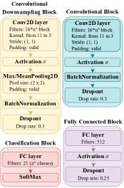
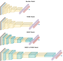
Figure 1: Overview of the Baseline model and corresponding blocks used for the study and its variants Wide, Deep, and Deep&Wide. A generic activation function $\sigma$ is used.

Table 1: Baseline architecture: input-output spatial dimensions, reported in the [Channels, Height, Width] format, and number of trainable parameters (N° Param.) of each layer in the case of a $256\times 256$ input.

Operations sequence	Input Shape	Output Shape
	[C,H,W]	[C,H,W]
Convolutional Downsamplig Block1	(3, 256, 256)	(16, 123, 123)
Convolutional Downsamplig Block2	(16, 123, 123)	(32, 57, 57)
Convolutional Downsamplig Block3	(32, 57, 57)	(64, 25, 25
Convolutional Downsamplig Block4	(64, 25, 25)	(128, 10, 10))
Convolutional Downsamplig Block5	(128, 10, 10)	(256, 4, 4)
Fully Connected Block	(256, 4, 4)	(512, 1, 1)
Classification Block	(512, 1, 1)	($N$, 1, 1)

The Wide, Deep, and Deep&Wide architectures are detailed below, while a block diagram for each designed architecture is shown in Figure 1.

• The Wide model is designed by doubling the dimension of the output of each Conv2D layer, i.e. the number of output filters of the Baseline model in the convolution.

• The Deep model is designed by doubling the number of convolutional operations, i.e. stacking to each CDB a further Convolutional Block (CB), as reported in Figure 1 (blue blocks), performing the same operations as the CDB except for the downsampling step of the 2D-max/mean pooling.

• The Deep&Wide model is designed by combining the previous Wide and Deep structures.

Finally, in order to assess the generality of the computational results, tests have been carried out also using two well-known neural architectures: Resnet50 (He et al (2016)) and Mobilenetv2 (Sandler et al (2018)). Resnet50 is a deep convolutional neural network with 50 hidden layers and with residual connections at each layer, meaning that the output of each layer is added to the output of the subsequent layer in order to prevent the well-known vanishing gradient issue (Borawar and Kaur (2023)). Mobilenetv2 is a lightweight convolutional neural network, which uses a ligher convolutional operator. Both Resnet50 and Mobilenetv2 are among the most used neural architectures for image classification.

4 The optimization problem for the Synthetic networks

The optimization problem related to our task consists in the unconstrained minimization of the Categorical Cross Entropy (CCE) between the predicted output of the neural model $\hat{y}^{j}_{i}(\omega)$ and the correct classes $y^{j}\in\{0,1\}^{N}$.

The predicted value $\hat{y}^{j}_{i}(\omega)$ is the output of the last Classification block, and it represents the probability, estimated by the neural architecture, that the sample $j$ belongs to class $i$. Thus, we have $\sum_{i=1}^{N}\hat{y}^{j}_{i}(\omega)=1\ \forall j=1,\dots,P\ \forall\omega\in\mathbb{R}^{h}$. Thus, the unconstrained optimization problem can be written as:

$$\min_{\omega\in\mathbb{R}^{h}}f(\omega):=-\frac{1}{P}\sum^{P}_{j=1}\sum^{N}_{i=1}y^{j}_{i}\log(\hat{y}^{j}_{i}(\omega))$$ (1)

We aim to derive the probability output of the Baseline synthetic network as a function of the network parameters $\omega$, i.e., $\hat{y}^{j}_{i}(\omega)$, and, in particular, to write the dependency of $\hat{y}^{j}_{i}$ from $\omega$ in a closed form

As reported in Figure 1, in the Baseline model the input images propagate along convolutional downsampling layers (CDB), a fully connected (FCB) and a classification (CB) layers. We formalize this process to get an analytical expression for $\hat{y}^{j}_{i}(\omega)$.

Each CDB performs five operations: a standard 2D-convolution, denoted as Conv2D layer in Figure 1, followed by an activation function, a Max-pooling or a Mean-pooling operation, the batch normalization. In the FCB, the Max/Mean-pooling is removed.

The input $X^{\ell-1}$ to a Conv2D layer $\ell$ is a tensor of dimension $[d^{\ell-1},m^{\ell-1},m^{\ell-1}]$ where $d^{\ell-1}$ are the channels and $m^{\ell}$ is the height/width of each channel $c=1,\dots,d^{\ell-1}$, and the output $X^{\ell}$ is a tensor of dimension $[d^{\ell},m^{\ell},m^{\ell}]$. The input $X^{0}$ at layer $\ell=0$ of the CDB layer is the colourful sample image represented with $m^{0}=256$ pixels and $d^{0}=3$ colour channels (red, green, blue). We denote by $X^{\ell}_{c}$ the matrix $m^{\ell}\times m^{\ell}$ for each channel $c=1,\dots,d^{\ell}$ and by $x_{c}=X^{0}_{c}\in\mathbb{R}^{m\times m}$ for $c=1,\dots,d^{0}$. A Conv2D layer $\ell$ applies a discrete convolution on the input $X^{\ell-1}$. This operation consists in applying filters (also called kernels) $w^{k}_{c}\in\mathbb{R}^{n\times n}$ for $k=1,\dots,d^{\ell}$ to the $c$-th input channel $X^{\ell-1}_{c}$ with $c=1,\dots,d^{\ell-1}$.

The convolution operation depends on the integer stride $s\geq 1$, representing the amount by which the filter $w^{k}_{c}$ shifts around the input $X^{\ell-1}_{c}$. The stride is commonly set to $s=1$, as we did for all the experiments except for L-BFGS for which the stride has been fixed to $s=2$. The dimension of the filter $n$, the number of channels $d^{\ell}$, and the stride $s\geq 1$, for each layer $\ell$, are network hyperparameters. Let us denote as $\otimes_{s}$ the discrete convolution operation with stride $s\in\mathbb{N}$. The expression componentwise of the convolutional operation between the filter $w^{k}_{c}\in\mathbb{R}^{n\times n}$ and the input feature $X^{\ell-1}_{c}$ is

$$\left[w^{k}_{c}\otimes_{s}X_{c}\right]_{ij}=\sum_{a=1}^{n}\sum_{b=1}^{n}[w^{k}_{c}]_{a,b}[X_{c}]_{i+sa,j+sb}\quad i,j=0,\dots,m-n$$

where for the sake of simplicity, we avoid the use of the superscript $\ell$. As reported in Bengio et al (2017) Chapter 9 (equation (9.4) with $s=1$), the $k$-th convoluted output is the matrix $F_{k}^{\ell}\in\mathbb{R}^{\frac{(m^{\ell-1}-n+1)}{s}\times\frac{(m^{\ell-1}-n+1)}{s}}$ defined as the sum over the channels, namely

$$F^{\ell}_{k}=\sum_{c=1}^{d^{\ell-1}}w^{k}_{c}\otimes_{s}X^{\ell-1}_{c}\qquad k=1,\dots,{d^{\ell}}$$ (2)

The convoluted output $F^{\ell}$ of the Conv2D layer $\ell$ is thus

$$F^{\ell}=[F^{\ell}_{k}]_{k=1,\dots,d^{\ell}}=(F^{1},\dots,F^{d^{\ell}})\in\mathbb{R}^{d^{\ell}\times\frac{(m^{\ell-1}-n+1)}{s}\times\frac{(m^{\ell-1}-n+1)}{s}},$$

The parameters of the convolutional layer $\ell$ are denoted as

$$W_{Conv}^{\ell}=\left[w^{k}_{c}\right]^{k=1,\dots,d^{\ell}}_{c=1,\dots,d^{\ell-1}}\in\mathbb{R}^{n\times n\times d^{\ell}\times d^{\ell-1}}$$ (3)

The next block applies a nonlinear activation function $\sigma$ to the output of the Conv2D layer $\ell$. The activation function $\sigma$ that has been used in the computational experiments in Section 8 can be either the ReLU $\sigma(z)=\max\{0,z\}$ or the SiLU $\sigma(z)=\frac{z}{1+e^{-z}}$ (Mercioni and Holban (2020); Ramachandran et al (2017)). In particular, the SiLU is used when applying L-BFGS to ensure the smoothness of the objective function and avoid failures of the optimization procedure.

In CDB blocks, the Conv2D output is submitted to the pooling operation aimed at further reducing the image dimensionality. The pooling operation Pool involves sliding a two-dimensional non-overlapping $p\times p$ matrix, where $p$ is the pool size, over each convoluted output $F^{\ell}_{k}$ and contracting the features lying within the $p\times p$ region covered by the filter by using the max or the mean operation. More formally, let us introduce the set ${\cal P}_{(i,j)}$ of positions i.e., for each $(i,j)$ the rows and columns of the matrix $F^{\ell}_{k}$, that are located in the $p\times p$ region; then Pool: $F^{\ell}_{k}\to G^{\ell}_{k}$ where the $k$-th pooled output is $G^{\ell}_{k}\in\mathbb{R}^{\frac{(m^{\ell-1}-n+1)}{sp}\times\frac{(m^{\ell-1}-n+1)}{sp}}$ . The output of the Max-Pool or Mean-Pool layer is computed respectively as:

$$(G_{k})^{Max}_{ij}=\max_{(r,c)\in{\cal P}_{(i,j)}}(F_{k})_{r,c}\qquad\qquad(G_{k})^{Mean}_{ij}=\frac{1}{\left|{\cal P}_{(i,j)}\right|}\sum_{(r,c)\in{\cal P}_{(i,j)}}(F_{k})_{r,c}$$ (4)

where for the sake of simplicity we removed the superscript $\ell$. The set ${\cal P}_{(i,j)}$ depends on how drastically we want to reduce the dimensionality. In our experiments, we have set $p=2$. In this case, the moving region is just a $2\times 2$ matrix, thus we halve the dimension of $F$. For instance, ${\cal P}_{(1,1)}=\{(1,1),(1,2),(2,1),(2,2)\}$, meaning that $G_{11}^{k}$ is the maximum/mean value between four different values $\{F^{k}_{1,1},F^{k}_{1,2},F^{k}_{2,1},F^{k}_{2,2}\}$. The Max-pooling operation is widely used in image classification, but it introduces a non-differentiability issue. For this reason, when testing L-BFGS, where differentiability is crucial, we use the Mean-pooling.

The output of a CDB block obtained by Equation 2 and Equation 4 is $Z^{\ell}=\left\{\texttt{Pool}\left[\sigma\left(Z^{\ell}_{k}\right)\right]\right\}_{k=1,\dots,d_{\ell}}$ and finally given as

$$Z^{\ell}=\left\{\texttt{Pool}\left[\sigma\left(F^{\ell}_{k}\right)\right]\right\}_{k=1,\dots,d_{\ell}}$$ (5)

whereas the output of a CB block does not use the Pool operations and thus is given simply by $Z^{\ell}=F^{\ell}$. In both cases, $Z^{\ell}$ is then normalized to stabilize and speed up the training process. The normalization is performed following the standard batch-normalization procedure described in Ioffe and Szegedy (2015), i.e., subtracting the mean and dividing by the standard deviation.

The output of the last layer $X^{L}$, being $L$ the total number of layers, of either CDB or CB is finally sent into the Fully Connected Block (FCB) and then into the Classification Block. The FCB is a shallow Feed-forward Neural (FFN) Network with $M_{FCB}$ neural units and the activation function $\sigma$ (ReLU or SiLU, as before). The output of the FCB is given by:

$$Z_{FCB}=\sigma(W_{FCB}^{T}X^{L}+b_{FCB})$$ (6)

where $(W_{FCB},b_{FCB})$ are the weights and the biases of the FFN network. The Classification Block is made up of a shallow FFN network followed by a softmax operation, so that the final output is

$$\hat{y}=\texttt{Soft}(Z_{CB})=\texttt{Soft}\left(W_{CB}^{T}Z_{FCB}+b_{CB}\right)$$ (7)

where Soft is applied component-wise to the vector $Z_{CB}$ as

$$\texttt{Soft}(z_{h})=\frac{e^{z_{h}}}{\sum_{j=1}^{N}e^{z_{j}}}.$$

The overall network parameters are

$$\omega=(W_{CB},b_{CB},W_{FCB},b_{FCB},W_{Conv}^{L},\dots,W_{Conv}^{1}).$$

Mobilenetv2 (Sandler et al (2018)) and the Resnet50 (He et al (2016)) presnets differences with respect to the Synthetic Network. Indeed, Mobilnetv2 instead uses depthwise separable convolutions different from (2), while Resnet50 presents residual connections among layers. Thus, the resulting optimization problem can be different with respect to the one described in this section.

5 The selected optimization algorithms

In this paper, L-BFGS and eight state-of-the-art ML optimization algorithms with multiple hyperparameters setups are compared. Precisely, those are: Adam (Kingma and Ba (2015)), Adamax (Kingma and Ba (2015)), Nadam (Dozat (2016)), RMSprop, SGD (Robbins and Monro (1951); Bottou et al (2018); Ruder (2016); Sutskever et al (2013b)), FTRL (McMahan (2011)), Adagrad (Duchi et al (2011)), and Adadelta (Zeiler (2012)). We use the SciPy version for L-BFGS and the built-in implementation in TensorFlow library for the eight others.

For the sake of completeness, we report the updating rule of each algorithm, assuming it is applied to the problem as in Equation 1, namely

$$\min_{\omega\in\mathbf{R}^{h}}f(\omega)=\sum_{p=1}^{P}f_{p}(\omega).$$

We note that all algorithms require $f$ to be a continuously differentiable function. The use of non-differentiable activation functions (ReLU) in the network layers and the MaxPooling layer, as usually done in CNN, implies that the objective function $f$ does not satisfy this essential property and a finite number of non-differentiable points arise. When using L-BFGS, this aspect becomes evident as discussed in the Section 8.1. We tried to use L-BFGS with the standard setting in CNNs, but it happened very often that the method failed and ended at a non-stationary point. Indeed, since L-BFGS is a full-batch method using all the samples at each iteration, whenever a point of non-differentiability is reached, the gradient returned by TensorFlow is None, and the method gets stuck. The other eight first-order algorithms are instead mini-batch methods, which perform network parameters update using only a small subset of the whole samples. When it happens that the partial gradient is None on a subset of samples, the method continues in the epoch, changing the batch and possibly the new partial gradient can be used to move from the current iteration. Hence, although convergence of the mini-batch methods requires smoothness, from the computational point of view they can work heuristically without it.

Hence when using L-BFGS, we need to reduce non-differentiability. To this aim we set SiLU as activation function and we select the MeanPooling, which is not a common practice in CNN for image classification. We also fully deactivate the Dropout operation and set stride s = 2. We also remark that we are comparing a globally convergent traditional full-batch method with eight different mini-batch methods, that require strong assumptions to prove convergence that do not hold for the problem at hand. By studying L-BFGS performance against commonly used optimizers we aim to assess whether theoretical convergence really plays an important role in determining the efficiency, the train performances, and, most of all, the generalization capability.

5.1 L-BFGS

Being one of the best-known first-order methods with strong convergence properties (see Liu and Nocedal (1989)), L-BFGS belongs to the limited memory quasi-Newton methods class. This algorithm is purely deterministic and, at every iteration $k$, exploits an approximated inverse Hessian of the objective function, and it performs the following update scheme:

$$\omega_{k+1}=\omega_{k}-\eta_{k}H_{k}\nabla f(\omega_{k})$$

where $\eta_{k}$ is a step size obtained via some line search method.

The updating rule for $H_{k}$ has been formalized by Nocedal and Wright (1999). Given an initial approximate Hessian $H_{0}\sim\left[\nabla^{2}f(\omega_{0})\right]^{-1}$, the algorithm uses the rule:

$$H_{k+1}=V^{T}_{k}H_{k}V_{k}+\frac{s_{k}s^{T}_{k}}{y_{k}^{T}s_{k}}$$

where

$$s_{k}=\omega_{k+1}-\omega_{k},\qquad y_{k}=\nabla f(\omega_{k+1})-\nabla f(\omega_{k}),\quad V_{k}=I-\frac{y_{k}s^{T}_{k}}{y_{k}^{T}s_{k}},$$

being $I$ is the identity matrix.

L-BFGS is not among the optimizers mostly used in machine learning. However, in force of its strong convergence properties, this algorithm has recently gained increasing interest in the research community. Some multi-batch versions of L-BFGS have been proposed in the past years in (Berahas et al (2016); Bollapragada et al (2018); Berahas and Takáč (2020)), in particular for image processing tasks in medicine in (Yun et al (2018); Wang et al (2019)).

Since L-BFGS is not directly available in TensorFlow, we have used the SciPy version implemented with an open-source wrapper available online.

5.2 SGD

The Stochastic Gradient Descent (SGD) is the basic algorithm to perform the minimization of the objective function using a direction $d^{k}$ which is random estimate of its gradient (see for details, the comprehensive survey Bottou et al (2018)). In the TensorFlow implementation, the following mini-batch approximation is used:

$$g_{k}(\omega_{k})=\displaystyle\frac{1}{|{\cal B}_{k}|}\sum_{i\in{\cal B}_{k}}\nabla f_{i}(\omega_{k})\text{ for some }{\cal B}_{k}\subset\{1,\dots,P\}$$

The updating rule is given by

$$\omega_{k+1}=\omega_{k}-\eta_{k}g_{k}(\omega_{k})$$

The update step can be modified by adding a momentum term (which depends on a parameter $\beta$) or a Nesterov acceleration step which are an extrapolation steps along the difference between the two past iterations. TensorFlow allows the use of a boolean parameter, called Nesterov, which enables the Nesterov acceleration step (see Sutskever et al (2013a)). When Nesterov=False, only a momentum is applied and the basic SGD iteration is modified by adding

$$\beta_{k}(\omega_{k}-\omega_{k-1})$$

with $\beta_{k}\geq 0$ momentum parameter. When Nesterov=True, first

$$z_{k}=\omega_{k}+\beta_{k}(\omega_{k}-\omega_{k-1})$$ (8)

is computed and the updating rule becomes

$$\omega_{k+1}=z_{k}-\eta_{k}g_{k}(z^{k}).$$

In both cases, the value of $\beta$ is a hyperparameter to be tuned.

In Bertsekas and Tsitsiklis (2000) the pure SGD has been proved to converge to a stationary point under strong assumptions. We further refer the reader to Drori and Shamir (2020) for a thorough analysis of SGD complexity and convergence rate.

5.3 Adam

Adam is one of the first SGD extensions, where the gradient estimate is enhanced with the use of an exponential moving average according to two coefficients: $\beta_{1}$ and $\beta_{2}$, ranging in $(0,1)$. The index $i\in\{1,2\}$ is referred to as the moment of the stochastic gradient, i.e., the first moment (expected value) and the second moment (non-centred variance). Being $g_{k}$ the same mini-batch approximation used in SGD,we define the following first and second-moment estimators at iterate $k$:

$$\mathbb{E}\left[\nabla f(\omega_{k})\right]\sim m_{k}=(1-\beta_{1})\sum_{i=1}^{k}\beta_{1}^{k-i}g_{i}$$ (9)

$$\mathbb{E}^{2}\left[\nabla f(\omega_{k})\right]\sim v_{k}=(1-\beta_{2})\sum_{i=1}^{k}\beta_{2}^{k-i}{(g_{i}\odot g_{i})}$$ (10)

where $\odot$ is the Hadamard component-wise product among vectors.

Given the following matrix:

$$\widetilde{V}_{k}(\varepsilon)=\frac{1}{1-\beta_{2}^{k}}\left[I\varepsilon+\mbox{diag}({v}_{k})\right]^{\frac{1}{2}}$$

where $\mbox{diag}(v)$ denotes the diagonal $h\times h$ matrix with elements $v_{i}$ on the diagonal, and $\epsilon>0$, the updating rule is the following:

$$\omega_{k+1}=\omega_{k}-\eta_{k}\widetilde{V}_{k}(\varepsilon)^{-1}\frac{1}{1-\beta_{1}^{k}}m_{k}$$

where $m_{k}$ is given in (9). It has been recently proved in Défossez et al (2020) that Adam can converge under smoothness assumption and gradients boundness in $L_{\infty}$ norm with convergence rate $O(\frac{h\log(N)}{N})$, being $h$ the number of variables and $N$ the numbers of iterations. For a more detailed discussion of Adam complexity (as well as for the other adaptive gradient methods Adamax and Nadam), we refer the reader to Zhou et al (2018).

5.4 Adamax

Adamax performs mainly the same operations described in Adam, but it does not make use of the parameter $\epsilon$, and the algorithm exploits the infinite norm to average the gradient. Let

$$u_{k}=\max_{i=1,\dots,k}\beta_{2}^{k-i}|g_{i}|\qquad U_{k}=\mbox{diag}(u_{k})$$

and $m_{k}$ as in (9). Thus, the updating rule is:

$$\omega_{k+1}=\omega_{k}-\eta_{k}U_{k}^{-1}\frac{1}{(1-\beta_{1}^{k})}m_{k}.$$

5.5 Nadam

Nadam, also known as Nesterov-Adam, performs the same updating rule as Adam but employs the Nesterov acceleration step Equation 8. Nadam is expected to be more efficient, but the Nesterov trick involves only the order in which operations are carried out and not the updating formula.

5.6 Adagrad

Adagrad is the first Adam extension that makes use of adaptive learning rates to discriminate more informative and rare features. The general update rule of $\omega_{k}\in\mathbf{R}^{h}$ involves complex matrix operations, for which we need to introduce some other notation. At iteration $k$ we introduce the cumulative vector

$$G_{k}=\displaystyle\sum_{t=0}^{k-1}\left(g_{t}\odot g_{t}\right)$$

where $g_{t}=\sum_{i\in{\cal B}_{t}}\nabla f_{i}(\omega_{t})$. Given $\varepsilon>0$ and the identity matrix $I$, we define the following matrix:

$$H_{k}(\varepsilon)=\left[I\varepsilon+\mbox{diag}(G_{k})\right]^{\frac{1}{2}}$$

where $\mbox{diag}(v)$, where $v\in\mathbf{R}^{h}$, denotes the diagonal ${h\times h}$ matrix with elements $v_{i}$ on the diagonal. Thus, the updating rule resulting after the minimization of a specific proximal function (see Duchi et al (2011)) is the following:

$$\omega_{k+1}=\omega_{k}-\eta H_{k}(\varepsilon)^{-1}g_{k}$$

Convergence results concerning Adagrad, as well as its modification Adadelta, have been reported in (Li and Orabona (2019); Défossez et al (2020); Chen et al (2018)) and they still require strong assumptions.

5.7 RMSProp

Proposed by Hinton et al. in the unpublished lecture Hinton et al (2012), RMSProp (Root Mean Square Propagation) performs a similar operations as Adagrad, but the update rule is modified to slow down the learning rate decrease.

In particular, following the notation introduced in the last subsections, at iteration $k$ the following matrix is used:

$${V}_{k}(\varepsilon)=\left[I\varepsilon+\mbox{diag}({v}_{k})\right]^{\frac{1}{2}}$$

where $v_{k}$ be given by (10). The update rule is:

$$\omega_{k+1}=\omega_{k}-\eta{V_{k}(\varepsilon)^{-1}}g_{k}$$

Despite being still unpublished, RMSProp has already been studied in the field of convergence theory in (Défossez et al (2020); De et al (2018)), with an eye to the non-convex ML context.

5.8 Adadelta

Adadelta (Zeiler (2012)) can be considered as an extension of Adagrad, which allows for a less rapid decrease in learning rate. Let us consider the same matrix

$${V}_{k}(\varepsilon)=\left[I\varepsilon+\mbox{diag}({v}_{k})\right]^{\frac{1}{2}}$$

used in RMSProp. Further, let $\delta_{k}=\omega_{k+1}-\omega_{k}$

$${\widetilde{\delta}}_{k}=\displaystyle\sum_{t=1}^{k}\rho^{k-t}(1-\rho)\left(\delta_{t}\odot\delta_{t}\right)\qquad\widetilde{\Delta}_{k}(\varepsilon)=\left[I\varepsilon+\mbox{diag}({\widetilde{\delta}}_{k})\right]^{\frac{1}{2}}$$

Thus, we can write the Adadelta updating rule as follows:

$$\omega_{k+1}=\omega_{k}-V_{k}(\varepsilon)^{-\frac{1}{2}}\widetilde{\Delta}_{k-1}(\varepsilon)g_{k}$$

5.9 FTRL

FTRL (Follow The Regularized Leader), as implemented in TensorFlow following McMahan et al (2013), is a regularized version of SGD, which uses the L1 norm to perform the update of the variables. Given, at every iteration $k$, $d_{k}=\sum_{t=1}^{k}g_{t}$, and fixed the quantity $\sigma_{k}$ such that $\sum_{t=0}^{k}\sigma_{t}=\frac{1}{\eta_{k}}$, the update rule is the following:

$$\omega_{k+1}=\arg\min_{\omega}\{d_{k}^{T}\omega+\sum_{t=1}^{k}\sigma_{t}||\omega-\omega_{t}||^{2}+\lambda||\omega||_{1}\}$$

As proved in McMahan et al (2013), the minimization problem in the update rule can be solved in closed form, setting:

$$\omega_{k+1,i}=\begin{cases}0\ \ \ \text{if }|z_{k,i}|\leq\lambda\\ -\eta_{k}(z_{k,i}-\texttt{sgn}(z_{k,i})\lambda)\text{ otherwise}\end{cases}$$ (11)

where $\displaystyle z_{k,i}=d_{k}-\sum_{s=1}^{k}\sigma_{s}\omega_{s}$ and $\texttt{sgn}(\cdot)$ is the Signum function.

FTLR convergence can be proved only in the convex case, as explained in detail in McMahan (2011).

6 The datasets

We have carried out our computational test using three datasets: UC Merced (Yang and Newsam (2010)), CIFAR10 and CIFAR100 (Krizhevsky et al (2009)). UC Merced represents the benchmark dataset used to define the Baseline problem, namely the training of the Baseline network defined in Section 3. We use the Baseline problem (defined as the pair Baseline network - UC Merced) to assess the performance of the different optimization methods.

UC Merced is a balanced dataset that comprises a total of 2100 land samples divided into 21 classes, i.e. 100 images per class. The dataset images have a resolution of $256\times 256$ pixels. The high number of classes and the limited number of samples for each class make the multi-class classification a non-trivial task.

In order to assess whether the computational results obatined on the Baseline problem generalize to different datasets, we have also carried out additional tests on two larger datasets: CIFAR10 and CIFAR100 (Krizhevsky et al (2009)), respectively, with $N=$10 and $N=$100 classes, both containing 60000 samples at a resolution of $H\times W=32\times 32$ pixels.

Furthermore, for minibatch methods, we also apply data augmentation, which is a commonly used technique in machine learning for image classification. It consists of random transformation of the selected mini-batch of samples with the aim of increasing the training dataset diversity and achieving better generalization capabilities. For a better understanding of this technique, we refer the reader to (Van Dyk and Meng, 2001; Connor and Khoshgoftaar, 2019); in our case, data augmentation involves random transformations on selected images, such as rotation, scaling, adding noise, and changing brightness and contrast.

7 Implementation details

We implemented the proposed study using TensorFlow 2 deep learning high-level API, using its implementation of Categorical Cross Entropy (CCE). We set the environment seed (also for the normal initializer of the convolutional kernels) at a randomly chosen value equal to 1699806 or to a specific list of values in the multistart analysis. Computational tests have been conducted using a mini-batch size $bs=128$, except for L-BFGS, which is a batch method, i.e., requires the whole gradient at each iteration. Concerning the eight built-in optimizers, in Section 8.1 the network was trained setting to 100 the number of epochs over the whole dataset. We remark that a single epoch consists of $\frac{P}{bs}$ update steps, being $P$ the number of samples in the dataset. In the experiments with tuned hyperparameters in Section 8.2, we halved the number of epochs. In other experiments with larger problems, the number of epochs was further reduced to 30. We underline that reducing the number of epochs is a common heuristic procedure in deep learning (Diaz et al (2017); Yu and Zhu (2020)), where at an early testing phase the number of epochs is set to an arbitrary value (in our case 100) and, then, it is reduced according to the training loss decrease, such that the network is not trained when the loss has already reached values close to zero and is not further improving. This prevents any waste of computational time that could result from training the network when the loss is already extremely close to zero.

Eventually, we underline that the TensorFlow implementation of the eight built-in optimizers, as well as the SciPy version of L-BFGS, uses back-propagation algorithm to compute the gradients.

The training have been run on 12GB NVIDIA GTX TITAN V GPU. The L-BFGS algorithm, being a full-batch method, cannot be run on a GPU due to the lack of memory storage, and takes almost 30 seconds on our reference Intel i9-10900X CPU to execute an entire step, i.e. a batch containing all the training samples.

8 Computational Results

We present in this chapter our computational experiments divided into three blocks. In Section 8.1, we explain how we have tested L-BFGS and the eight optimizers briefly described in Section 5 on the baseline problem, i.e., training the Baseline architecture on UC Merced dataset, using default setting of the hyperparameters. We have also carried out a multistart test on the three worst-performing algorithms (Adadelta, Adagrad, and FTLR) to assess whether poor performances were caused only by an unfortunate weights initialization or by the inherent behaviour of these optimizers on the dataset. We discuss the correlation between the test accuracy performances and the precision with which the problem in Equation 1 is solved, the loss profiles produced by the algorithms, as well as the role of the data augmentation technique. Our further analysis in the following sections is focused only on five of these optimizers since, as shown in Section 8.1, they achieved the highest accuracy prediction. In Section 8.2, we describe the grid search we have carried out on the baseline network on UC Merced dataset to tune optimizers’ hyperparameters. We show how a careful tuning aimed at finding a nearly-optimal hyperparameters setting can result in significant improvements in terms of test accuracy. In Section 8.3, we discuss the results obtained after modifying the network architecture with respect to the baseline, investigating in particular hyperparameters robustness to the increase in depth and width.

Finally, in Section 8.4, we carry out tests on the two other image classification datasets, CIFAR10 and CIFAR100 with $H=W=32$ pixels and $N=10,100$ respectively.

Table 2: Number of trainable parameters (variables) of the different neural architectures; they depend on $H,W,N$. The values are reported in millions [M].

Architecture	# variables [M]
	UCMerced	CIFAR10	CIFAR100
Baseline	4.84	0.72	0.74
Wide	10.97	2.72	2.74
Deep	9.83	1.57	1.62
Deep & Wide	22.52	5.99	6.05
Resnet50	24.77	24.77	24.79
Mobilenetv2	3.05	3.05	3.07

8.1 The Baseline problem with default hyperparameters

The first tests we have carried out are aimed at studying the optimizers’ performances both from an optimization perspective (i.e., the value of the final loss) and a machine learning perspective (i.e., the test accuracy). Hyperparameters have been set to their default values (Table 3), taken from the TensorFlow documentation.

Table 3: Default and tuned values of the TensorFlow built-in optimizer hyperparameters. The tuned values are reported in brackets when different from the default ones, The grid search has not been performed for the worst-performing algorithms: Adadelta, Adagrad, and FTRL.

Algorithm	SGD	Adam	Adamax	Nadam	RMSProp	Adadelta	Adagrad	FTRL
$\eta$	$10^{-2}(10^{-1})$	$10^{-3}$	$10^{-3}$	$10^{-3}$	$10^{-2}\ (10^{-3})$	$10^{-3}$	$10^{-3}$	$10^{-3}$
$\beta$	0 (0.9)	-	-	-	0	-	-	0.1
$\beta_{1}$	-	0.9	0.9 (0.6)	0.9 (0.99)	-	-	-	0
$\beta_{2}$	-	0.999 (0.9999)	0.999 (0.99)	0.999 (0.99)	-	-	-	0
$\epsilon$	-	$10^{-7}\ (10^{-8})$	$10^{-7}\ (10^{-6})$	$10^{-7}\ (10^{-6})$	$10^{-7}\ (10^{-6})$	$10^{-7}$	$10^{-7}$	-
Amsgrad	-	False (True)	-	-	-	-	-	-
$\rho$	-	-	-	-	0.9	0.95	0.95	-
Centered	-	-	-	-	False	-	-	-
Nesterov	False	-	-	-	-	-	-	-

For each algorithm, we report in Figure 2 the behaviour of the training losses without and with data augmentation,a and in Table 4 the test accuracy.

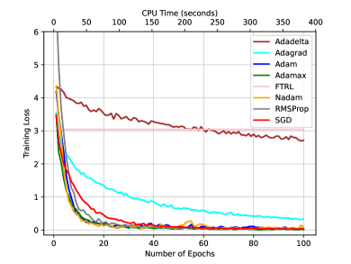
((a)) W/out data augmentation

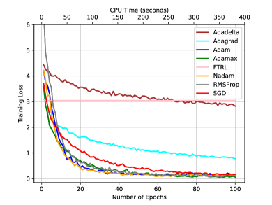
((b)) with data augmentation

Figure 2: Training loss for the baseline problem with default hyperparameters setting: (a) without data augmentation and (b) with data augmentation. A colour is assigned to each algorithm according to the legend.

We noticed that, while most of the algorithms converge to points in the neighbourhood of the globally optimal solution, i.e., the training loss is close to zero, Adadelta, Adagrad, and FTRL get stuck in some local minima, as can be seen in Figure 2. This results in quite poor accuracy performances for Adadelta, Adagrad, and FTRL as reported in the first column of Table 4. We highlight that FTRL is an extreme case, being the descent so slow that the loss profile looks like an horizontal line. This is not surprising because, as explained in McMahan et al (2013), FTRL has been thought to deal with extremely sparse datasets, which is not the case for colored images. Furthermore, FTLR convergence requires a very strong convexity condition (McMahan (2011)), making it impossible to predict its behaviour in such a non-convex context.

Table 4: Test accuracy in % obtained with default values and with tuned values ($\pm$ % increase) of the optimization algorithms, without data augmentation (W/out DA) and with data augmentation (with DA).

Algorithm	Adam	Adamax	Nadam	RMSProp	SGD	Adadelta	Adagrad	FTRL
W/out DA	60.0 % (+2.1 %)	61.3 % (+1.7 %)	61.3% (+3.0 %)	60.2% (+3.1 %)	59.4 % (+1.8%)	17.6 %	32.7 %	4.6 %
With DA	72.4 % (+2.5 %)	72.5 % (+0.0 %)	72.1 % (+2.6 %)	74 % (-1.9 %)	65.1 % (+4.4 %)	18.0 %	31.0 %	4.6 %

The observed behaviour seems to confirm what has been already pointed out in (Swirszcz et al (2016); Yun et al (2018)): neural networks can be affected by the local minima issue, which has a direct influence on the performance metrics. Getting stuck in bad local minima often implies also an accuracy level that makes the entire network useless for the classification task. In the case of FTRL, the test accuracy is so low that the network selects randomly the predicted class.

Furthermore, data augmentation has no substantial effect in modifying the convergence endpoint. Indeed, Adadelta, Adagrad, and FTRL are somehow stable in returning the a bad point, as well as SGD, Adam, Adamax, Nadam, and RMSProp always converge to good solutions, leading to similar values of accuracy, as we can see again in Table 4. Nonetheless, data augmentation have a boosting effect on test accuracy for all five working algorithms. This improvement is obtained because data augmentation artificially increases the diversity and the quantity of the training data and, thus, enhances the network generalization capability. Nonetheless, data augmentation also makes the task harder and thus the the training loss decrease is slightly slower, i.e., the network needs more time to learn.

In order to investigate the behaviour of Adadelta, Adagrad, and FTRL and to assess the stability of their bad performance, we have carried out another test employing a multistart procedure. To this aim we have initialized the weights using two different distributions Glorot Uniform (GU) (Glorot and Bengio, 2010) and Lecun Normal (LN) (LeCun et al, 1989) and 16 different seed values, i.e., starting from 16 different initial points for each initialization, that is from 32 different points in total. The three algorithms always get stuck in a point, with value of the training loss quite far from zero with respect to the others. This behaviour is very stable and does not change with the initialization seeds.

Best accuracy values, not reported in a table for the sake of brevity, are always $4.6\%$ for FTRL, $18.2\%$ for Adadelta, and $32.7\%$ for Adagrad. These results suggest that the bad behaviour of Adadelta, Adagrad, and FTRL is not just caused by an unfortunate initial point. These algorithms seem to converge to points which are not good for our classification task. Hence, we have discarded Adadelta, Adagrad, and FTRL from the testing phases reported in the next sections.

Concerning L-BFGS, we use the original dataset without data augmentation (which is specific for mini-batch methods). We have first trained the baseline problem using the ReLU as activation function, as well as the MaxPooling Equation 4 and the Dropout operations. Since the final points returned by L-BFGS are influenced by the starting point (Liu and Nocedal (1989)), we ran the algorithm with different initialization seeds. In particular, we have used again the Glorot Uniform and Lecun Normal distributions and, due to the heavy computational effort, only 5 different seed values for each initialization. The training loss profile of this first set of experiments are reported in Figure 3(a). We observe that the algorithm always fails before achieving convergence: the lines in Figure 3(a) stop because the returned loss was infinite at a given iteration. We argue that this is caused by a non-differentiability issue. Indeed, as we already discussed, L-BFGS convergence is guaranteed exclusively when the objective function is continuously differentiable (Liu and Nocedal (1989)) and the ReLU, as well as the MaxPooling operation Equation 4, cause the occurrence of non-differentiable points, i.e., points where the gradient is not defined. Although, this could in principle happen with any other algorithm, since L-BFGS is a full-batch method, once a non-differentiable point is reached the algorithm gets stuck.

Hence, we have also trained the baseline network in a more differentiable setting, namely using the SiLU activation function, the MeanPooling and disabling the Dropout operation. As we show in Figure 3(b), results significantly improved with almost all the initialization seeds. However, the loss does not always tend to zero and L-BFGS generally converges to points with a far worse loss function value than Adam, Adamax, Nadam, RMSProp, and SGD.

This difference can be seen also in terms of test accuracy. Indeed, when using the MaxPooling layers and the ReLU activation function, L-BFGS performs quite poorly in terms of test accuracy reaching the maximum value of $15.4\%$.

When using the ”differentiable” setting, we obtain better results reported in Table 5. We report the average over the 5 runs of the final training loss values and of the test accuracies. We observe that even the most unlucky initialization, which is GU 10, results in a test accuracy of 15,6% which is better than the highest one obtained with ReLU and MaxPooling. However, L-BFGS is much more sensible to the initialization seed with respect to the other built-in methods, confirming claim ii). The final training loss, as well as the test accuracy, are not stable and may vary in a wide range of values. Despite this computational result could question the practical effectiveness of traditional batch methods in deep learning, it also confirms our claim i): the quality of local minima matters. Indeed, looking at Table 5, we observe a relation between the final loss value and the test accuracy: lower final loss value usually corresponds to higher test accuracy. In general, the accuracy performances achieved are not satisfactory when compared to mini-batch methods as well as the training loss decrease in unstable and highly influenced by the starting point. Finally, we also remark that L-BFGS is significantly less efficient with respect to the other built-in algorithms. Indeed, it is practically impossible to run it on a standard GPU, because one needs enough memory storage to access the entire dataset in one single step, which is possible only on CPU and this results in slower training.

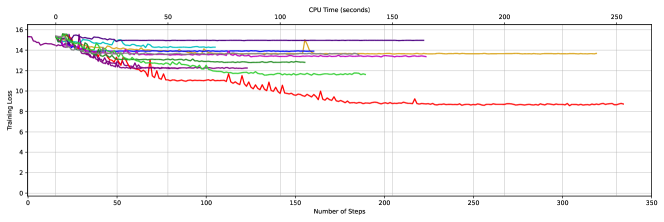
((a)) Using ReLU activation function, MaxPooling and Dropout operations

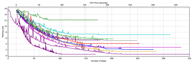
((b)) Using SiLU activation function, MeanPooling and without Dropout and using Conv with 2 strides

Figure 3: L-BFGS training loss with 5 different initialization seeds as reported in the legend, using the Lecun Normal (LN) and Glorot Uniform (GU) initialization procedures.

Table 5: Average value of the training loss (Avg Train value) and Average Test accuracy in % (Avg Test acc) obtained on the baseline problem with L-BFGS in the ”differentiable” setting on 10 multistart runs using 5 different seeds for the two different distributions GU and LN: different training loss results in different test performances.

Seed	$0$		$10$		$100$		$1000$		$1699806$
Distribution	LN	GU	LN	GU	LN	GU	LN	GU	LN	GU
Avg Train value	4.17	2.80	1.49	5.30	2.10	12.16	7.12	5.73	0.48	5.13
Avg Test acc	37.6%	51.3%	43.8%	15.6%	27.6%	16.5%	27.1%	23.3%	49.8%	35.2%

8.2 Impact of tuning on the Baseline problem

In this section, we perform tuning of hyperparameters of the optimization algorithm on the baseline problem, namely on the baseline architecture and the UC Merced problem, to assess their role in the computational efficiency and, in turn, on the final test accuracy. As we mentioned in the introduction, default values for hyper-parameters are often obtained by maximizing the aggregated (in most cases the average) performance across a variety of different tasks, balancing a trade-off between efficiency and adaptability to different datasets (Probst et al (2019); Yang and Shami (2020); Bischl et al (2023)). We aim here to assess if a specific tuning on the classification task has a influence on algorithms’ behavior. As this will be the case, in the next section we analyse the impact of the tuning obtained on a baseline problem to other settings (architecture and/or dataset).

We discard Adadelta, Adagrad, FTRL, and L-BFGS from further analysis due to their extremely poor performance on the baseline problem. Thus, we have carried out a grid search to tune the hyperparameters of Adam, Adamax, Nadam, RMSProp, and SGD on the baseline problem.

The grid search ranges are reported in Table 6. Concerning numerical hyperparameters, we have chosen ranges centered in the default values, resulting in almost 200 possible combinations for each algorithm. We did not perform either a $k$-fold cross-validation or a multistart procedure, as is usually the case in computer vision (see e.g., (Gärtner et al (2023))) for computational reasons. Indeed, each run (including loading the dataset and the network to the GPU and the effective computational time) takes approximately 9 minutes (around 2 seconds per epoch plus the set-up time). Thus, performing the grid search over about 200 hyperparameter settings takes 1.25 days on a fully dedicated 12GB NVIDIA GTX TITAN V GPU for each of the five algorithms. This implies that each training phase with a complete grid search would require nearly 6.25 days. Therefore, performing, e.g. a $k$-fold cross-validation would require $6.25\cdot k$ days on a fully dedicated machine, being a prohibited amount of time for standard values of $k$ (5 or 10). Similar observations holds for a multistart procedure.

Table 6: Range of the grid search for the different hyperparameters. For the sake of brevity, we have omitted the boolean hyperparameters, Amsgrad for Adam, Centered for RMSProp, and Nesterov for SGD.

Algorithm	Adam	Adamax	Nadam	RMSProp	SGD
$\eta$	$10^{-i},i=2,3,4$	$10^{-i},i=2,3,4$	$10^{-i},i=2,3,4$	$10^{-i},i=2,3,4$	$10^{-i},i=1,2,3,4$
$\beta$	-	-	-	$\{0,0.5,0.9\}$	$\{0,0.5,0.9\}$
$\beta_{1}$	$\{0.6,0.9,0.99\}$	$\{0.6,0.9,0.99\}$	$\{0.6,0.9,0.99\}$	-	-
$\beta_{2}$	$\{0.99,0.999,0.9999\}$	$\{0.99,0.999,0.9999\}$	$\{0.99,0.999,0.9999\}$	-	-
$\epsilon$	$[10^{-i},i=6,7,8]$	$[10^{-i},i=6,7,8]$	$[10^{-i},i=6,7,8]$	$[10^{-i},i=6,7,8]$	-
$\rho$	-	-	-	$\{0.6,0.9,0.99\}$	-

The tuned values of the hyperparameters are selected considering the best test accuracy obtained and are reported into brackets in Table 3, when different from default ones. Once tuned the hyperparameters to new values, we have used them on the Baseline problem halving the number of epochs.

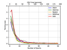
((a)) W/out data augmentation

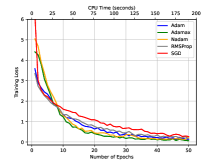
((b)) with data augmentation

Figure 4: Training loss with tuned hyperparameters values for the baseline problem: (a) without data augmentation,(b) with data augmentation.

We report in Figure 4(a) and Figure 4(b) the training loss profiles for the two settings without data augmentation and with data augmentation. Comparing with the corresponding training loss with default values in Figure 2(a) and Figure 2(b), we can state that tuning does not directly influence the final value of the objective function returned by the algorithms, which was already the global optimal value near to zero. However, the loss decrease is faster, and nearly optimal values (near to zero) are reached earlier, optaining good results despite having halved the number of epochs. In particular, in Figure 4(a) the loss is almost zero already after 15-20 epoch, while in Figure 2(a) after 25-30 epochs. Considering the case with data augmentation, in Figure 2(b) the loss is almost zero after 40 epochs in Figure 4(b) the same is true after approximately 60 epochs.

However, our computational experience shows that the most relevant benefit of hyperparameters tuning is the gain in terms of test accuracy. In Table 4 we report in square brackets the test accuracy changes for the five optimizers, with and without data augmentation.The change is always positive except for RMSProp with data augmentation. We also observe that Adam, SGD and Nadam show a larger improvement over Adamax and RMSProp both w/out and with data augmentation.

8.3 Impact of tuning when changing the architectures

In this section, we aim to investigate the impact of tuned vs default hyperparameters when changing the network architecture whilst the dataset is UC Merced.

In particular, we are interested in assessing how optimizers react to the increase in depth and width, using the three synthetic configurations (Wide, Deep, Deep&Wide) described in Section 3, as well as in determining the impact of tuning the hyperparameters on state-of-the-art architectures as Resnet50, and Mobilenetv2.

In this experiment, we perform a single run for each algorithm starting from the same initial point, fixing the distribution and the random seed to LN 1699806, and considering the use of data augmentation, which gave better results in the former experiments.

The results for the synthetic architectures are reported in Figure 5 (training results) and in Table 7 (test accuracy), whereas the results for the state-of-the-art architectures are in Figure 6 (training) and Table 8 (test). In Table 9, we report a cumulative difference in test accuracy (TEST ACC) when using Tuned versus Default hyperparameters setting on average for the Synthetic Networks.

In terms of training loss, on the synthetic networks, the tuned version seems to reach, on average, slightly smaller values, whereas on the state-of-the.art architectures, there are not noticeable differences in the reached value. Thus, the tuning of the hyperparameters does not improve significantly the decrease rate.

As regard the test accuracy on synthetic networks, in Table 7 we report for each algorithm the % accuracy obtained for UCMerced dataset on the four different architectures and also the average % over the architectures (column Avg ARCH).

From Table 7, it seems that SGD and Adamax benefit from the tuned setting on the synthetic architectures, significantly improving the average of the % accuracy (Avg ARCH), whereas Adam and Nadam are slightly worse on average. RMSProp deteriorates significantly, but we remark that this was the only case of worst performance also in the Baseline problem with data augmentation (see Table 4). These results are confirmed by the absolute difference between the tuned and default average test accuracy reported in Table 9 where SGD and Adam obtain the higher and significant increase.

The accuracy on Resnet50 and Mobilenetv2 are reported in % in Table 8 and with absolute variation in Table 9. On these architectures, the tuned configuration does not perform uniformly better. However, we observe an improvement when using SGD on Mobilenetv2, which is more similar in the architecture to the Baseline architecture. Thus, we can conclude that when the architecture is significantly different from the Baseline used for tuning Hyperparmeters, the advantages are limited.

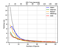
((a)) Wide - Default HP

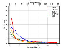
((b)) Wide - Tuned HP

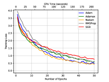
((c)) Deep - Default HP

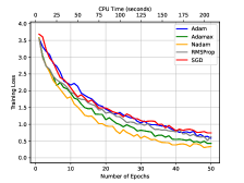
((d)) Deep - Tuned HP

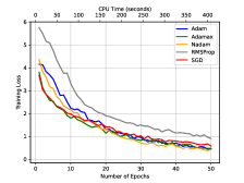
((e)) Deep&Wide - Default HP

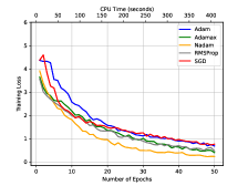
((f)) Deep&Wide - Tuned HP

Figure 5: Training Loss trends of the 5 algorithms for UC Merced on the synthetic architectures.

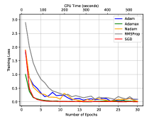
((a)) Resnet50 - Default HP

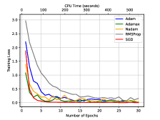
((b)) Resnet50 - Tuned HP

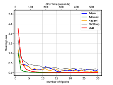
((c)) Mobilenetv2 - Default HP

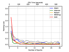
((d)) Mobilenetv2 - Tuned HP

Figure 6: Training Loss trends of the 5 algorithms for UC Merced on Resnet50 and Mobilenetv2.

8.4 Impact of tuning when changing the datasets

In this last set of experiments, we aim to assess the role of tuning when training all the architectures on the two additional datasets CIFAR10 and CIFAR100, described in Section 6.

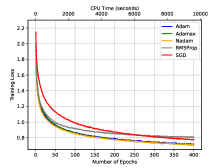
((a)) Default HP - Baseline

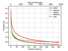
((b)) Tuned HP - Baseline

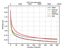
((c)) Wide - Default HP

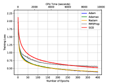
((d)) Wide - Tuned HP

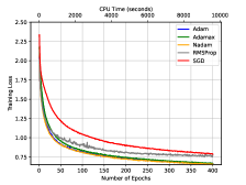
((e)) Deep - Default HP

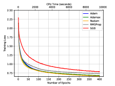
((f)) Deep - Tuned HP

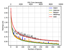
((g)) Deep&Wide - Default HP

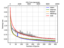
((h)) Deep&Wide - Tuned HP

Figure 7: Training Loss trends of the 5 algorithms for CIFAR10 on the synthetic architectures.

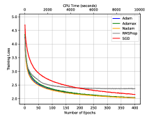
((a)) Default HP - Baseline

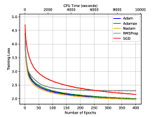
((b)) Tuned HP - Baseline

((c)) Default HP - Wide

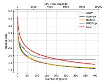
((d)) Tuned HP - Wide

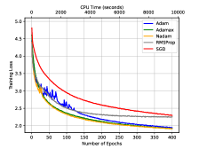
((e)) Default HP - Deep

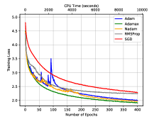
((f)) Tuned HP - Deep

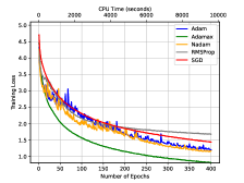
((g)) Default HP - Deep&Wide

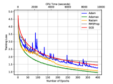
((h)) Tuned HP - Deep&Wide

Figure 8: Training Loss trends of the 5 algorithms for CIFAR100 on the synthetic architectures.

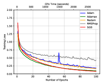
((a)) Resnet50 - Default HP

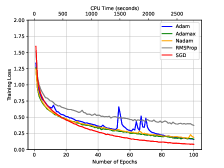
((b)) Resnet50 - Tuned HP

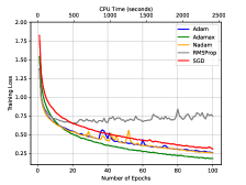
((c)) Mobilenetv2 - Default HP

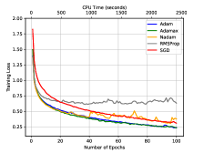
((d)) Mobilenetv2 - Tuned HP

Figure 9: Training loss trends for CIFAR10 on Resnet50 and MobilenetV2.

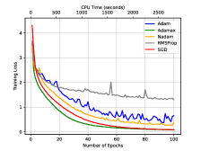
((a)) Resnet50 - Default HP

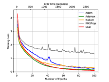
((b)) Resnet50 - Tuned HP

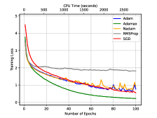
((c)) Mobilenetv2 - Default HP

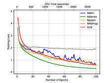
((d)) Mobilenetv2 - Tuned HP

Figure 10: Training Loss trends of the 5 algorithms for CIFAR100 on Resnet50 and MobilenetV2.

The training loss on CIFAR 10 are reported in fig. 7 and Figure 9 for the synthetic architectures and for the state-of-the-art architectures respectively, whereas the results on CIFAR100 are in Figure 8 and Figure 10. The test accuracies are reported in % in Table 7 and Table 8 (test), and as the absolute difference between tuned and default version in Table 9.

Looking at the training losses both on CIFAR10 and CIFAR100, we do not observe significant differences in the profile of the training loss for most of the architectures among the two configurations, default or tuned one.

Considering that in almost all the tests, regardless of the architecture and the dataset, the final value of the training loss is not remarkably different between the tuned and the default case, one could conclude that the optimal hyper-parameters setting found in Section 8.2 on the Baseline network is not robust enough. Nonetheless, if we move to the generalization performance, measured by the final test accuracy, things appear differently.

Indeed, looking at Table 7 and Table 8, we observe that SGD presents a strong advantage of the tuned configuration, while average accuracy values are often very close to each other for the other optimizers. SGD is the only non-adaptive optimizer, meaning that the learning rate is not adjusted during the training. We argue that this makes SGD much more sensitive to the hyper-parameters setting than other adaptive algorithms. Nonetheless, even on Adam and Nadam, the tuned configuration achieves slightly better test accuracy. A remarkable exception to this pattern is Resnet50 in Table 8, where the default configuration significantly outperforms the tuned one. This result seems to suggest that our hyper-parameter configuration found on the baseline is not robust to more radical architectural changes, like in Resnet50, where residual connections (see Section 3) are added to each layer to prevent the vanishing gradient effect. Nonetheless, the overall average effect of using the tuned configuration instead of the default is positive, as it is shown in the last row of Table 9. Summing up positive and negative contributions, the average improvement in terms of test accuracy is almost $2\%$ with the only exception of Resnet architecture.

Table 7: Test accuracy in % obtained by training the synthetic network architectures using the Default and Tuned hyperparameter values. For each algorithm in the two settings, we report the average over the datasets when the architecture is fixed (Avg DATA) and the average over the architecture when the Dataset is fixed (Avg ARCH).

		Default					Tuned
	DATASET	Baseline	Wide	Deep	DeepWide	Avg ARCH	Baseline	Wide	Deep	DeepWide	Avg ARCH
Adam	UC Merced	72,4	65,1	56	61,9	63,9	74,9	70,3	51,7	48,6	61,4
	CIFAR10	77,2	82,3	77,6	85,3	80,6	77,6	83,2	79,4	86,2	81,6
	CIFAR100	48,8	54,3	46,4	50,2	49,9	48,6	54,7	47,4	49,7	50,1
	Avg DATA	66,1	67,2	60,0	65,8		67,0	69,4	59,5	61,5
Adamax	UC Merced	72,5	68,2	18,3	30,5	47,4	72,5	67,8	58,2	64,1	65,7
	CIFAR10	77,7	82,5	78,7	86,4	81,3	77,8	82,7	78,9	84,9	81,1
	CIFAR100	46,8	55	47,5	55,5	51,2	47,3	55,4	46,2	55,9	51,2
	Avg DATA	65,7	68,6	48,2	57,5		65,9	68,6	61,1	68,3
Nadam	UC Merced	72,1	70,8	51,3	60,1	63,6	73,7	73,8	39,7	59	61,6
	CIFAR10	78,7	82,7	77	85,4	81,0	78,8	82,6	79,5	86,6	81,9
	CIFAR100	47,1	55,3	46,9	52	50,3	48,9	53,9	47,1	53,2	50,8
	Avg DATA	66,0	69,6	58,4	65,8		67,1	70,1	55,4	66,3
RMSProp	UC Merced	70.4	65,2	58,9	52,5	61,8	72,1	64,2	28,1	44,3	52,2
	CIFAR10	77,2	82,8	78,6	84,2	80,7	76,1	80,2	77,6	83,7	79,4
	CIFAR100	44,8	51,2	44,6	55,1	48,9	47,1	51,8	45,9	55,5	50,1
	Avg DATA	64,1	66,4	60,7	63,9		65,1	65,4	50,5	61,2
SGD	UC Merced	65,1	63,2	24,3	23,3	44,0	69,5	63,2	51,4	56,8	60,2
	CIFAR10	75,1	81,3	75,5	77	77,2	75,1	80,7	74,9	82,9	78,4
	CIFAR100	46,9	55,1	35,8	53,9	47,9	46,9	54,9	40,6	52,5	48,7
	Avg over DATA	62,4	66,5	45,2	51,4		63,8	66,3	55,6	64,1

Table 8: Test accuracy in % obtained by training the Resnet50 and Mobilenetv2 using the Default and Tuned hyperparameter values. For each algorithm in the two settings, we report the average over the datasets when the architecture is fixed (Avg DATA) and the average over the architecture when the Dataset is fixed (Avg ARCH).

		Default			Tuned
	DATASET	Resnet50	Mobilenetv2	Avg ARCH	Resnet50	Mobilenetv2	Avg ARCH
Adam	UC Merced	84,8	23,3	54,1	91,9	24,6	58,3
	CIFAR10	93	69	81,0	74,8	64	69,4
	CIFAR100	42,9	39	41,0	45,3	40,3	42,8
	Avg DATA	73,6	43,8	58,7	70,7	43,0	56,8
Adamax	UC Merced	93	69	81,0	74,8	64	69,4
	CIFAR10	82,4	81,7	82,1	83,3	80,6	82,0
	CIFAR100	51,2	45,1	48,2	49	47,9	48,5
	Avg DATA	75,5	65,3	70,4	69,0	64,2	66,6
Nadam	UC Merced	90,8	18,7	54,8	86,2	15,5	50,9
	CIFAR10	82,8	81,2	82,0	83,1	80,4	81,8
	CIFAR100	44,2	35,4	39,8	44,3	33,4	38,9
	Avg DATA	72,6	45,1	58,9	71,2	43,1	57,2
RMSProp	UC Merced	70,5	18,3	44,4	78,7	8,7	43,7
	CIFAR10	80,7	36,2	58,5	80,3	40,5	60,4
	CIFAR100	25	18,5	21,8	42,6	21,9	32,3
	Avg DATA	58,7	24,3	41,5	67,2	23,7	45,5
SGD	UC Merced	97	69,2	83,1	74,8	97	85,9
	CIFAR10	81,7	70	75,9	81,7	79,9	80,8
	CIFAR100	51,2	48,6	49,9	51,2	48,6	49,9
	Avg DATA	76,6	62,6	69,6	69,2	75,2	72,2

Table 9: Differences in test accuracy (TEST ACC) of Tuned vs Default hyperpameters setting when training the Resnet50, Mobilenetv2 and on average for the Synthetic Networks. Positive (negative) values indicate better performance of the tuned (default) setting.

		TEST ACC TUNED - TEST ACC DEFAULT
	DATASET	Resnet50	Mobilenetv2	Avg Synthetic Net.
Adam	UC Merced	7,10	1,30	-2,48
	CIFAR10	-18,20	-5,00	1,00
	CIFAR100	2,40	1,30	0,18
	Avg over DATA	-2,90	-0,80	-0,43
Adamax	UC Merced	-18,20	-5,00	18,28
	CIFAR10	0,90	-1,10	-0,25
	CIFAR100	-2,20	2,80	0,00
	Avg over DATA	-6,50	-1,10	6,01
Nadam	UC Merced	-4,60	-3,20	-2,03
	CIFAR10	0,30	-0,80	0,92
	CIFAR100	0,10	-2,00	0,45
	Avg over DATA	-1,40	-2,00	-0,22
RMSProp	UC Merced	8,20	-9,60	-10,48
	CIFAR10	-0,40	4,30	-1,30
	CIFAR100	17,60	3,40	1,15
	Avg over DATA	8,47	-0,63	-3,54
SGD	UC Merced	-22,20	27,80	16,25
	CIFAR10	0,00	9,90	1,18
	CIFAR100	0,00	0,00	0,80
	Avg over DATA	-7,40	12,57	6,08
OVERALL AVERAGE		-1,95	1,61	1,58

8.5 Collective impact of tuning: performance profiles

In this section, we consider a collective representation of the training results with the aim of assessing the impact of tuned versus default setting in reaching the global solution. Following the underlying idea of the bench-marking method proposed in (Dolan and Moré, 2002) and (Moré and Wild, 2009), we consider a variant of the performance profiles as an additional tool of comparison between the five algorithms: Adam, Adamax, Nadam, RMSProp, and SGD.

Following (Moré and Wild, 2009), given the set of problems $\mathcal{P}$ and the set of solvers $\mathcal{S}$, a problem $p\in\mathcal{P}$ is solved by a solver $s\in\mathcal{S}$ with precision $\tau$ if

$$f(\omega_{p,s})\leq f^{p}_{L}+\tau(f(\omega^{0}_{p})-f^{p}_{L}),$$

being $\omega^{0}_{p}$ the starting point of problem $p\in\mathcal{P}$, which is the same for all solvers, $f(\omega_{p,s})$ the final value of the objective function in (1) after the training process and $f^{p}_{L}=\min_{s\in\mathcal{S}}f(\omega_{p,s})$. In our case $\mathcal{P}$ is made up of the 18 different versions of the problem (1) corresponding to all the possible combinations of the 6 network architectures (Baseline, Deep, Wide, Deep&Wide, Resnet50, Mobilenetv2), with the three datasets. Further, in our set of experiments we have fixed the epochs, i.e. the computational time. Hence differently from (Moré and Wild, 2009), we are interested in checking how many problems are solved to a given accuracy $\tau$. Thus we introduce the success rate performance profile $\sigma_{s}(\tau)$ for a solver $s$ in Figure 11 as:

$$\sigma_{s}(\tau)=\frac{1}{|\mathcal{P}|}|\{p\in P:f(\omega_{p,s})\leq f^{p}_{L}+\tau(f(\omega^{0}_{p})-f^{p}_{L})\}|.$$

In Figure 11 we plot $\sigma_{s}(\tau)$ with $\tau\in[10^{-4},1]$. The higher the plot on the left, the better. Looking at the performance profiles in Figure 11, we confirm that it is not possible to state the superiority of the tuning versions in the training performance. However, the tuned versions of the algorithms differ less from each other, being more stable.

8.6 Data availability

All the data we have presented in this section are fully reproducible from the source code, which is available on the public Github repository at https://github.com/lorenzopapa5/Computational_Issues_in_Optimization_for_Deep_networks.

((a)) Default HP

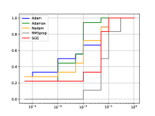
((b)) Tuned HP

Figure 11: Success rate performance profiles $\sigma_{s}(\tau)$ of the five algorithms $s$ on the 18 problems arising by considering all the 6 architectures over all the three datasets: a) with default and b) tuned hyper parameters settings

9 Conclusions

In this paper, nine optimization open-source algorithms have been extensively tested in training a deep CNN network on a multi-class classification task. Computational experience shows that not all the algorithms reach a neighbourhood of a global solution, and some of them get stuck in local minima, independently of the choice of the starting point. Algorithms reaching a local non-global solution have test performances, i.e., accuracy on the test set, far below the minimal required threshold for such a task. This result confirms the initial claim that reaching a neighbourhood of a global optimum is extremely important for generalization performance.

A fine grid search on the optimization hyperparameters leads to hyperparameter choices that give remarkable improvements in test accuracy when the network structure and the dataset do not change. Thus, using a default setting might not be the better choice.

Finally, the tests on different architectures and datasets suggest that when the architectural changes are not too radical, it could be convenient to use the tuned configuration than the default one. We believe that this result can have a remarkable impact, especially on ML practitioners asked to train similar models on different datasets belonging to the same problem class, e.g., image classification, which is often the case in real-world applications. Performing a grid-search on a representative problem of a given class and tuning the hyperparameters on it instead of using the default configuration can be seen as creating a new customized setting, which is reusable for larger instances and achieves better generalization performance.

References

- \bibcommenthead
- Abbaschian et al (2021) Abbaschian BJ, Sierra-Sosa D, Elmaghraby AS (2021) Deep learning techniques for speech emotion recognition, from databases to models. Sensors (Basel, Switzerland) 21
- Advani et al (2020) Advani MS, Saxe AM, Sompolinsky H (2020) High-dimensional dynamics of generalization error in neural networks. Neural Networks 132:428–446
- Baumann et al (2019) Baumann P, Hochbaum DS, Yang YT (2019) A comparative study of the leading machine learning techniques and two new optimization algorithms. European journal of operational research 272(3):1041–1057
- Bengio et al (2017) Bengio Y, Goodfellow I, Courville A (2017) Deep learning, vol 1. MIT press Cambridge, MA, USA
- Berahas and Takáč (2020) Berahas AS, Takáč M (2020) A robust multi-batch L-BFGs method for machine learning. Optimization Methods and Software 35(1):191–219
- Berahas et al (2016) Berahas AS, Nocedal J, Takác M (2016) A multi-batch L-BFGS method for machine learning. Advances in Neural Information Processing Systems 29
- Bertsekas and Tsitsiklis (2000) Bertsekas DP, Tsitsiklis JN (2000) Gradient convergence in gradient methods with errors. SIAM Journal on Optimization 10(3):627–642
- Bertsimas and Dunn (2017) Bertsimas D, Dunn J (2017) Optimal classification trees. Machine Learning 106:1039–1082
- Bischl et al (2023) Bischl B, Binder M, Lang M, et al (2023) Hyperparameter optimization: Foundations, algorithms, best practices, and open challenges. Wiley Interdisciplinary Reviews: Data Mining and Knowledge Discovery 13(2):e1484
- Bollapragada et al (2018) Bollapragada R, Nocedal J, Mudigere D, et al (2018) A progressive batching L-BFGS method for machine learning. In: International Conference on Machine Learning, PMLR, pp 620–629
- Borawar and Kaur (2023) Borawar L, Kaur R (2023) Resnet: Solving vanishing gradient in deep networks. In: Proceedings of International Conference on Recent Trends in Computing: ICRTC 2022, Springer, pp 235–247
- Bottou et al (2018) Bottou L, Curtis FE, Nocedal J (2018) Optimization methods for large-scale machine learning. Siam Review 60(2):223–311
- Braiek and Khomh (2020) Braiek HB, Khomh F (2020) On testing machine learning programs. Journal of Systems and Software 164:110,542. https://doi.org/10.1016/j.jss.2020.110542, URL https://www.sciencedirect.com/science/article/pii/S0164121220300248
- Buntine (2020) Buntine W (2020) Learning classification trees. In: Artificial Intelligence frontiers in statistics. Chapman and Hall/CRC, p 182–201
- Carrizosa et al (2021) Carrizosa E, Molero-Río C, Romero Morales D (2021) Mathematical optimization in classification and regression trees. Top 29(1):5–33
- Chen et al (2018) Chen X, Liu S, Sun R, et al (2018) On the convergence of a class of Adam-type algorithms for non-convex optimization. arXiv preprint arXiv:180802941
- Connor and Khoshgoftaar (2019) Connor S, Khoshgoftaar TM (2019) A survey on image data augmentation for deep learning. Journal of big data 6(1):1–48
- De et al (2018) De S, Mukherjee A, Ullah E (2018) Convergence guarantees for RMSProp and Adam in non-convex optimization and an empirical comparison to nesterov acceleration. arXiv preprint arXiv:180706766
- Défossez et al (2020) Défossez A, Bottou L, Bach F, et al (2020) A simple convergence proof of Adam and Adagrad. arXiv preprint arXiv:200302395
- Diaz et al (2017) Diaz GI, Fokoue-Nkoutche A, Nannicini G, et al (2017) An effective algorithm for hyperparameter optimization of neural networks. IBM Journal of Research and Development 61(4/5):9–1
- Ding and Tao (2017) Ding C, Tao D (2017) Trunk-branch ensemble convolutional neural networks for video-based face recognition. IEEE transactions on pattern analysis and machine intelligence 40(4):1002–1014
- Ding et al (2022) Ding T, Li D, Sun R (2022) Suboptimal local minima exist for wide neural networks with smooth activations. Mathematics of Operations Research 47(4):2784–2814
- Dogo et al (2018) Dogo EM, Afolabi O, Nwulu N, et al (2018) A comparative analysis of gradient descent-based optimization algorithms on convolutional neural networks. In: 2018 International Conference on Computational Techniques, Electronics and Mechanical Systems (CTEMS), IEEE, pp 92–99
- Dolan and Moré (2002) Dolan ED, Moré JJ (2002) Benchmarking optimization software with performance profiles. Mathematical programming 91(2):201–213
- Dozat (2016) Dozat T (2016) Incorporating nesterov momentum into Adam. In: ICLR Workshop
- Drori and Shamir (2020) Drori Y, Shamir O (2020) The complexity of finding stationary points with stochastic gradient descent. In: International Conference on Machine Learning, PMLR, pp 2658–2667
- Duchi et al (2011) Duchi J, Hazan E, Singer Y (2011) Adaptive subgradient methods for online learning and stochastic optimization. Journal of machine learning research 12(7):2121–2159
- Gambella et al (2021) Gambella C, Ghaddar B, Naoum-Sawaya J (2021) Optimization problems for machine learning: A survey. European Journal of Operational Research 290(3):807–828
- Gärtner et al (2023) Gärtner E, Metz L, Andriluka M, et al (2023) Transformer-based learned optimization. In: Proceedings of the IEEE/CVF Conference on Computer Vision and Pattern Recognition, pp 11,970–11,979
- Geiger et al (2019) Geiger M, Spigler S, d’Ascoli S, et al (2019) Jamming transition as a paradigm to understand the loss landscape of deep neural networks. Physical Review E 100(1):012,115
- Glorot and Bengio (2010) Glorot X, Bengio Y (2010) Understanding the difficulty of training deep feedforward neural networks. In: Proceedings of the thirteenth international conference on artificial intelligence and statistics, JMLR Workshop and Conference Proceedings, pp 249–256
- Goodfellow et al (2014) Goodfellow IJ, Vinyals O, Saxe AM (2014) Qualitatively characterizing neural network optimization problems. arXiv preprint arXiv:14126544
- Guo et al (2018) Guo Y, Liu Y, Georgiou T, et al (2018) A review of semantic segmentation using deep neural networks. International journal of multimedia information retrieval 7(2):87–93
- Haji and Abdulazeez (2021) Haji SH, Abdulazeez AM (2021) Comparison of optimization techniques based on gradient descent algorithm: A review. PalArch’s Journal of Archaeology of Egypt/Egyptology 18(4):2715–2743
- He et al (2016) He K, Zhang X, Ren S, et al (2016) Deep residual learning for image recognition. 2016 IEEE Conference on Computer Vision and Pattern Recognition (CVPR) pp 770–778
- Hijazi et al (2015) Hijazi S, Kumar R, Rowen C, et al (2015) Using convolutional neural networks for image recognition. Cadence Design Systems Inc: San Jose, CA, USA 9
- Hinton et al (2012) Hinton G, Srivastava N, Swersky K (2012) Neural networks for machine learning lecture 6a overview of mini-batch gradient descent. Cited on 14(8):2
- Howard et al (2017) Howard AG, Zhu M, Chen B, et al (2017) Mobilenets: Efficient convolutional neural networks for mobile vision applications. ArXiv abs/1704.04861
- Huang et al (2017) Huang G, Liu Z, Weinberger KQ (2017) Densely connected convolutional networks. 2017 IEEE Conference on Computer Vision and Pattern Recognition (CVPR) pp 2261–2269
- Im et al (2016) Im DJ, Tao M, Branson K (2016) An empirical analysis of the optimization of deep network loss surfaces. arXiv preprint arXiv:161204010
- Ioffe and Szegedy (2015) Ioffe S, Szegedy C (2015) Batch normalization: Accelerating deep network training by reducing internal covariate shift. In: International conference on machine learning, pmlr, pp 448–456
- Jais et al (2019) Jais IKM, Ismail AR, Nisa SQ (2019) Adam optimization algorithm for wide and deep neural network. Knowledge Engineering and Data Science 2(1):41–46
- Kandel et al (2020) Kandel I, Castelli M, Popovič A (2020) Comparative study of first order optimizers for image classification using convolutional neural networks on histopathology images. Journal of imaging 6(9):92
- Kingma and Ba (2015) Kingma DP, Ba J (2015) Adam: A method for stochastic optimization. CoRR abs/1412.6980
- Krizhevsky et al (2009) Krizhevsky A, Nair V, Hinton G (2009) Cifar-10 (canadian institute for advanced research) URL http://www.cs.toronto.edu/~kriz/cifar.html
- Kuutti et al (2021) Kuutti S, Bowden R, Jin Y, et al (2021) A survey of deep learning applications to autonomous vehicle control. IEEE Transactions on Intelligent Transportation Systems 22:712–733
- Lan (2020) Lan G (2020) First-order and stochastic optimization methods for machine learning. Springer, New York
- LaValley (2008) LaValley MP (2008) Logistic regression. Circulation 117(18):2395–2399
- LeCun et al (1995) LeCun Y, Bengio Y, et al (1995) Convolutional networks for images, speech, and time series. The handbook of brain theory and neural networks 3361(10):1995
- LeCun et al (1989) LeCun Y, et al (1989) Generalization and network design strategies. Connectionism in perspective 19(143-155):18
- Lewis-Beck and Lewis-Beck (2015) Lewis-Beck C, Lewis-Beck M (2015) Applied regression: An introduction, vol 22. Sage publications
- Li et al (2018) Li H, Xu Z, Taylor G, et al (2018) Visualizing the loss landscape of neural nets. Advances in neural information processing systems 31
- Li and Orabona (2019) Li X, Orabona F (2019) On the convergence of stochastic gradient descent with adaptive stepsizes. In: The 22nd international conference on artificial intelligence and statistics, PMLR, pp 983–992
- Lim et al (2000) Lim TS, Loh WY, Shih YS (2000) A comparison of prediction accuracy, complexity, and training time of thirty-three old and new classification algorithms. Machine learning 40(3):203–228
- Liu and Nocedal (1989) Liu DC, Nocedal J (1989) On the limited memory BFGS method for large scale optimization. Mathematical programming 45(1):503–528
- McMahan (2011) McMahan B (2011) Follow-the-regularized-leader and mirror descent: Equivalence theorems and l1 regularization. In: Proceedings of the Fourteenth International Conference on Artificial Intelligence and Statistics, JMLR Workshop and Conference Proceedings, pp 525–533
- McMahan et al (2013) McMahan HB, Holt G, Sculley D, et al (2013) Ad click prediction: a view from the trenches. Proceedings of the 19th ACM SIGKDD international conference on Knowledge discovery and data mining
- Mercioni and Holban (2020) Mercioni MA, Holban S (2020) P-swish: Activation function with learnable parameters based on swish activation function in deep learning. In: 2020 International Symposium on Electronics and Telecommunications (ISETC), IEEE, pp 1–4
- Moré and Wild (2009) Moré JJ, Wild SM (2009) Benchmarking derivative-free optimization algorithms. SIAM Journal on Optimization 20(1):172–191
- Nocedal and Wright (1999) Nocedal J, Wright SJ (1999) Numerical optimization. Springer, New York
- Palagi (2019) Palagi L (2019) Global optimization issues in deep network regression: an overview. Journal of Global Optimization 73(2):239–277
- Papa et al (2022) Papa L, Alati E, Russo P, et al (2022) Speed: Separable pyramidal pooling encoder-decoder for real-time monocular depth estimation on low-resource settings. IEEE Access 10:44,881–44,890. 10.1109/ACCESS.2022.3170425
- Pisner and Schnyer (2020) Pisner DA, Schnyer DM (2020) Support vector machine. In: Machine learning. Elsevier, p 101–121
- Pouyanfar et al (2018) Pouyanfar S, Sadiq S, Yan Y, et al (2018) A survey on deep learning: Algorithms, techniques, and applications. ACM Computing Surveys (CSUR) 51(5):1–36
- Probst et al (2019) Probst P, Boulesteix AL, Bischl B (2019) Tunability: Importance of hyperparameters of machine learning algorithms. The Journal of Machine Learning Research 20(1):1934–1965
- Ramachandran et al (2017) Ramachandran P, Zoph B, Le QV (2017) Searching for activation functions. arXiv preprint arXiv:171005941
- Ranstam and Cook (2018) Ranstam J, Cook J (2018) LASSO regression. Journal of British Surgery 105(10):1348–1348
- Robbins and Monro (1951) Robbins H, Monro S (1951) A stochastic approximation method. The annals of mathematical statistics pp 400–407
- Rokach and Maimon (2010) Rokach L, Maimon O (2010) Classification trees. Data mining and knowledge discovery handbook pp 149–174
- Ruder (2016) Ruder S (2016) An overview of gradient descent optimization algorithms. arXiv preprint arXiv:160904747
- Sandler et al (2018) Sandler M, Howard A, Zhu M, et al (2018) Mobilenetv2: Inverted residuals and linear bottlenecks. In: Proceedings of the IEEE conference on computer vision and pattern recognition, pp 4510–4520
- Shorten et al (2021) Shorten C, Khoshgoftaar TM, Furht B (2021) Deep learning applications for COVID-19. Journal of Big Data 8
- Spigler et al (2019) Spigler S, Geiger M, d’Ascoli S, et al (2019) A jamming transition from under-to over-parametrization affects generalization in deep learning. Journal of Physics A: Mathematical and Theoretical 52(47):474,001
- Steinwart and Christmann (2008) Steinwart I, Christmann A (2008) Support vector machines. Springer Science & Business Media
- Sun (2019) Sun R (2019) Optimization for deep learning: theory and algorithms. arXiv preprint arXiv:191208957
- Sun et al (2020) Sun R, Li D, Liang S, et al (2020) The global landscape of neural networks: An overview. IEEE Signal Processing Magazine 37(5):95–108
- Sun et al (2019) Sun S, Cao Z, Zhu H, et al (2019) A survey of optimization methods from a machine learning perspective. IEEE transactions on cybernetics 50(8):3668–3681
- Suthaharan and Suthaharan (2016) Suthaharan S, Suthaharan S (2016) Support vector machine. Machine learning models and algorithms for big data classification: thinking with examples for effective learning pp 207–235
- Sutskever et al (2013a) Sutskever I, Martens J, Dahl G, et al (2013a) On the importance of initialization and momentum in deep learning. In: International conference on machine learning, PMLR, pp 1139–1147
- Sutskever et al (2013b) Sutskever I, Martens J, Dahl GE, et al (2013b) On the importance of initialization and momentum in deep learning. In: ICML
- Swirszcz et al (2016) Swirszcz G, Czarnecki WM, Pascanu R (2016) Local minima in training of neural networks. arXiv preprint arXiv:161106310
- Tatsumi and Tanino (2014) Tatsumi K, Tanino T (2014) Support vector machines maximizing geometric margins for multi-class classification. Top 22:815–840
- Van Dyk and Meng (2001) Van Dyk DA, Meng XL (2001) The art of data augmentation. Journal of Computational and Graphical Statistics 10(1):1–50
- Wang et al (2019) Wang H, Gemmeke H, Hopp T, et al (2019) Accelerating image reconstruction in ultrasound transmission tomography using L-BFGS algorithm. In: Medical Imaging 2019: Ultrasonic Imaging and Tomography, SPIE, pp 67–76
- Xu et al (2020) Xu P, Roosta F, Mahoney MW (2020) Second-order optimization for non-convex machine learning: An empirical study. In: Proceedings of the 2020 SIAM International Conference on Data Mining, SIAM, pp 199–207
- Yang and Shami (2020) Yang L, Shami A (2020) On hyperparameter optimization of machine learning algorithms: Theory and practice. Neurocomputing 415:295–316
- Yang and Newsam (2010) Yang Y, Newsam S (2010) Bag-of-visual-words and spatial extensions for land-use classification. In: Proceedings of the 18th SIGSPATIAL International Conference on Advances in Geographic Information Systems. Association for Computing Machinery, New York, NY, USA, GIS ’10, p 270–279, 10.1145/1869790.1869829, URL https://doi.org/10.1145/1869790.1869829
- Yu and Zhu (2020) Yu T, Zhu H (2020) Hyper-parameter optimization: A review of algorithms and applications. arXiv preprint arXiv:200305689
- Yun et al (2018) Yun C, Sra S, Jadbabaie A (2018) Small nonlinearities in activation functions create bad local minima in neural networks. arXiv preprint arXiv:180203487
- Zeiler (2012) Zeiler MD (2012) Adadelta: An adaptive learning rate method. ArXiv abs/1212.5701
- Zhang et al (2016) Zhang C, Bengio S, Hardt M, et al (2016) Understanding deep learning requires rethinking generalization. In: International Conference on Learning Representations
- Zhang et al (2021) Zhang C, Bengio S, Hardt M, et al (2021) Understanding deep learning (still) requires rethinking generalization. Communications of the ACM 64(3):107–115
- Zhou et al (2018) Zhou D, Chen J, Cao Y, et al (2018) On the convergence of adaptive gradient methods for nonconvex optimization. arXiv preprint arXiv:180805671