Testing for an Explosive Bubble using High-Frequency Volatility

Abstract

Based on a continuous-time stochastic volatility model with a linear drift, we develop a test for explosive behavior in financial asset prices at a low frequency when prices are sampled at a higher frequency. The test exploits the volatility information in the high-frequency data. The method consists of devolatizing log-asset price increments with realized volatility measures and performing a supremum-type recursive Dickey-Fuller test on the devolatized sample. The proposed test has a nuisance-parameter-free asymptotic distribution and is easy to implement. We study the size and power properties of the test in Monte Carlo simulations. A real-time date-stamping strategy based on the devolatized sample is proposed for the origination and conclusion dates of the explosive regime. Conditions under which the real-time date-stamping strategy is consistent are established. The test and the date-stamping strategy are applied to study explosive behavior in cryptocurrency and stock markets.

Keywords: Stochastic volatility model; Unit root test; Double asymptotics; Explosiveness; Asset price bubbles.

1 Introduction

In recent years, initiated by the influential paper by Phillips et al. (2011), there has been a renewed interest in the empirical identification of explosive behavior in financial asset prices as a means to detect economic bubbles. In Phillips et al. (2011), the test statistic is the supremum of recursively implemented Dickey-Fuller (DF) $t$-statistics, and a right-tailed test, referred to as the PWY test, is conducted. This approach effectively addresses the power deficiency commonly encountered in simple right-tailed unit root tests, a problem extensively discussed in prior studies such as Diba and Grossman (1987, 1988), Flood and Garber (1980), Flood and Hodrick (1986) and Evans (1991). When applied to price series after removal of fundamental components, the presence of explosiveness indicates the existence of a bubble phenomenon.

Subsequent studies have explored various theoretical and practical aspects of the bubble testing problem. For example, Phillips and Yu (2011) study the behavior of bubbles during the subprime crisis. Homm and Breitung (2012) propose various supremum-type tests for bubbles based on alternative tests for changes in persistence in time-series models. They also propose to use the supremum of backwardly implemented recursive Chow-type tests to test for bubbles. Phillips et al. (2015a) consider the problem of testing for multiple bubbles and propose a double supremum version of DF $t$-statistics over all possible subsamples as their test statistic. Phillips et al. (2015b) study the limit theory of bubble date detectors in the context of multiple bubbles. See also Harvey et al. (2017), Chong and Hurn (2015), Breitung and Kruse (2013), Pavlidis et al. (2017) and Shi and Song (2015), among others. These studies collectively contribute to advancing our understanding of bubble detection techniques and provide valuable insights into the dynamics and implications of explosive behavior in financial markets.

Existing research on testing asset price bubbles has predominantly been based on classical discrete-time autoregressive (AR) models, related to the unit-root-testing literature. However, in the finance literature, it is commonly assumed that asset prices follow a continuous-time model, which can offer analytical simplicity for pricing derivatives. Moreover, from an empirical modeling standpoint, continuous-time models provide a natural framework for incorporating data sampled at various frequencies, which is particularly relevant for the problem addressed in this paper.

In this study, we consider the problem of testing for explosive behavior within the framework of a continuous-time stochastic volatility model with a linear drift and nonparametric stochastic volatility. Unlike previous approaches, we do not assume that the stochastic volatility process satisfies the Markovian property. When the volatility is constant, our model corresponds to the well-known Ornstein-Uhlenbeck (OU) process. Testing for unit roots in the context of the OU process has been explored in prior works such as Phillips (1987), Perron (1991), Yu (2014), Zhou and Yu (2015) and Chen and Yu (2015). To capture the explosive behavior in the data, we allow the persistence parameter to vary from the unit root regime to the explosive regime. While the existing literature on bubble testing accounts for time-varying volatility, the proposed methods primarily focus on unconditional heteroskedasticity, as discussed in Harvey et al. (2016) and Harvey et al. (2020). However, relaxing the assumption of constant volatility and considering conditional heteroskedasticity and hence stochastic volatility is crucial, since volatility clustering is a stylized fact observed in asset prices.

Our testing procedure consists of two main steps. First, we utilize high-frequency data to estimate the integrated volatility over time intervals corresponding to a lower sampling frequency. This is achieved by employing the realized variance (RV) estimator, a widely used method in the literature (see, e.g., Andersen et al. (2001) and Barndorff-Nielsen and Shephard (2002)). Second, we “devolatize” the log-price increments at the lower frequency using the estimated realized volatility. Subsequently, we apply the strategy introduced by Phillips et al. (2011) (the PWY test strategy) to the devolatized series in order to test for explosive behavior in the data. We refer to this test as the RVPWY test. Under this framework, we show that the RVPWY statistic has the same asymptotic null distribution as the PWY statistic in the discrete-time model with a constant volatility. As a result, the critical values provided in Phillips et al. (2011) be readily utilized for inference in our RVPWY test.

Our proposed testing and date-stamping procedure involves applying the PWY test to a devolatized time series. This approach has significant implications for the outcomes of the testing and date-stamping procedure. To illustrate this idea, we plot the daily BitCoin log-prices from January 1, 2018 to August 31, 2021 in the left panel of Figure 1, and the devolatized log-price series (using the daily RV calculated from 5-minute returns) in the right panel, taken from our later empirical analysis. The differences between the two plots are striking. In the devolatized sample, sudden large drops in the BitCoin price are less apparent. Moreover, the magnitude of price decreases is considerably reduced, while the magnitude of price increases is largely preserved, making them more pronounced in a relative sense. This effect is primarily due to the higher volatility during periods of price drops in the original data. Since the devolatization strategy removes heteroskadasticity from the data, our intuition suggests that the devolatized sample provides a better foundation for more accurately identifying and date-stamping explosive behavior. This advantage is supported by our Monte Carlo simulations. Moreover, empirical analyses highlight some key differences between the proposed method and the existing method.

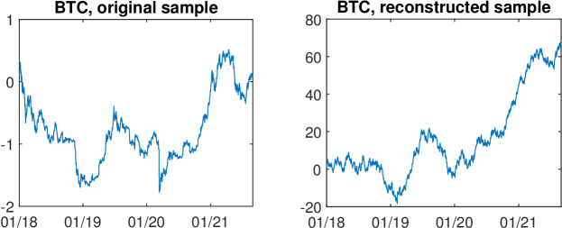
Figure 1: Log-price and pseudo log-price of BitCoin, January 1, 2018 to August 31, 2021

Empirically, existing tests for explosive bubbles (e.g. Phillips et al. (2011) and Phillips et al. (2015a)) are often applied to monthly asset prices. Widely available daily or intra-day asset price data are not used. Based on an empirically justifiable approximation strategy that we propose, we show that the methodology developed in this paper can be used to exploit the information of monthly volatility in asset price data from daily asset prices, which in turn help us in detecting explosiveness at the monthly frequency. In one of our empirical examples, we apply this idea to detect bubbles in the real S&P500 index.

In a similar vein, when the objective is to detect explosiveness in daily asset prices, having access to intra-day price data allows for accurate estimation of daily integrated volatility. By leveraging these highly precise daily volatility measures, we can enhance the reliability of our inference for explosiveness at the daily frequency. Consequently, our methodology offers a valuable tool for detecting and studying explosive behavior in daily asset prices. In our first empirical investigation, we apply our method to detect explosive behavior in cryptocurrencies at the daily level. Cryptocurrencies, being highly volatile assets, present an interesting and relevant context for studying explosiveness. By analyzing daily price data, we can gain insights into the presence and characteristics of potential explosive episodes in this market.

It is important to note that despite utilizing high-frequency intraday data in this paper, the primary interest lies in testing explosiveness at the low-frequency level, i.e. at the monthly or daily level. While it is theoretically possible to test for explosiveness in high-frequency data, the data-generating process at higher frequencies tends to be more complex compared to low-frequency data. Factors such as diurnal effects and market micro-structure noise need to be taken into account in high-frequency analyses, which can introduce complications that may invalidate existing methods. In practice, policymakers and investors often seek to understand whether an economic time series exhibits a bubble at the low-frequency level, even if they have access to high-frequency data. This preference can be attributed to various reasons, including the high costs associated with implementing new policies or rebalancing portfolios. As a result, our motivation is to test for explosiveness using low-frequency data, while assuming that higher-frequency data is available.

In terms of testing for explosiveness, the present paper is related to several strands of literature. First, it is related to Choi and Jarrow (2020), Jarrow and Kwok (2021) and Jarrow et al. (2022). In particular, Jarrow and Kwok (2023) propose to use quadratic variation only to identify explosive behavior in asset prices. Second, it is related to Andersen et al. (2023) where a different devolatizing technique and a different test were used. In particular, Andersen et al. (2023) use implied volatility obtained from options to devolatize the price series in the first stage and a CUSUM test was applied to the devolatized prices. Also, Andersen et al. (2023) assume that volatility follows a Markov process. Finally, our study is related to Phillips and Yu (2009b), where the realized volatility is used to estimate parameters in the diffusion function in the first stage of a two-stage approach. Related work, focusing on parameter estimation, is by Corradi and Distaso (2006) and Todorov (2009).

The structure of the paper is as follows. Section 2 considers a continuous-time model, defines the realized variance estimator, and discusses how to devolatize data. Section 3 considers the bubble testing problem, defines the RVPWY statistic, and derives the asymptotic null distribution. Section 4 performs Monte Carlo simulations to study the finite sample size and power properties of the proposed statistic, in comparison with currently available tests. Section 5 considers the real-time date-stamping problem. Section 6 applies the proposed methodology to two empirical datasets. Section 7 concludes the paper and discusses possible future research. Technical lemmas and mathematical proofs are collected in the Appendix.

Throughout the paper, we use $\xrightarrow{d}$ to denote convergence in distribution and use $\Rightarrow$ to denote weak convergence of a stochastic process. $\sim$ denotes “is distributed as”. $\lfloor x\rfloor$ denotes the integer part of a non-negative real number $x$.

2 The Model and Devolatizing Data

Consider the following continuous-time process with stochastic volatility for the log asset price process $\{y_{t}\}_{t\geqslant 0}$

$$\mathrm{d}y_{t}=\kappa y_{t}\mathrm{d}t+\sigma_{t}\mathrm{d}W_{t},\quad t\geqslant 0,$$ (1)

where $y_{0}=0$, $W$ is a Brownian motion process, $\sigma_{t}$ is a strictly positive stochastic volatility process, independent of the $W$ process, and $\kappa$ is the persistence parameter. Note that $\sigma_{t}$ is nonparametrically specified and need not satisfy the Markov property. In (1), $\kappa=0$ corresponds to the unit root model, and $\kappa>0$ corresponds to an explosive model. This model is an extension of the continuous-time Ornstein-Uhlenbeck (OU) model considered in Perron (1991) and Zhou and Yu (2015) to allow for stochastic volatility.

First, assume the asset price process $y_{t}$ is observed on a low-frequency time grid $t_{i}=iH$, where $i=0,1,2,\ldots,n$, and $H$ is the sampling interval (e.g., one day or one month). Discretizing model (1) at the observational frequency, we have

$$y_{t_{i}}-y_{t_{i-1}}=\kappa\int_{t_{i-1}}^{t_{i}}y_{u}\mathrm{d}u+\int_{t_{i-1}}^{t_{i}}\sigma_{u}\mathrm{d}W_{u}=\kappa\int_{t_{i-1}}^{t_{i}}y_{u}\mathrm{d}u+\sqrt{\int_{t_{i-1}}^{t_{i}}\sigma_{u}^{2}\mathrm{d}u}\times\varepsilon_{i},$$ (2)

$i=1,\ldots,n$, where $\varepsilon_{i}$ is defined as $\varepsilon_{i}:=\int_{t_{i-1}}^{t_{i}}\sigma_{u}\mathrm{d}W_{u}/\sqrt{\int_{t_{i-1}}^{t_{i}}\sigma_{u}^{2}\mathrm{d}u}$. Notice that this is an exact discretization: no approximation is used. Conditional on the $\sigma$ process, $\int_{t_{i-1}}^{t_{i}}\sigma_{u}\mathrm{d}W_{u}$ follows a $N(0,\int_{t_{i-1}}^{t_{i}}\sigma_{u}^{2}\mathrm{d}u)$ distribution, and hence $\varepsilon_{i}$’s are identically and independently distributed (i.i.d.) as $N(0,1)$. By the independence between $\sigma$ and $W$ process, we therefore have $\varepsilon_{i}\overset{\mathrm{i.i.d.}}{\sim}N(0,1)$, independent of $\sigma$. With these properties, the discretized model (2) can be read as a linear regression model of the sequence $\{y_{t_{i}}-y_{t_{i-1}}\}_{i=1}^{n}$ against $\{\int_{t_{i-1}}^{t_{i}}y_{u}\mathrm{d}u\}_{i=1}^{n}$ with coefficient $\kappa$, and with innovations given by the product of an i.i.d. standard normal sequence $\{\varepsilon_{i}\}_{i=1}^{n}$ and the daily conditional standard deviations $\{(\int_{t_{i-1}}^{t_{i}}\sigma_{u}^{2}\mathrm{d}u)^{1/2}\}_{i=1}^{n}$. In this paper, we follow the convention to refer to the quantity $\int_{t_{i-1}}^{t_{i}}\sigma_{u}^{2}\mathrm{d}u$ as the integrated variance and it square root as the integrated volatility.

Denote the unknown integrated volatility over the period from $t_{i-1}$ to $t_{i}$ as $\omega_{i}:=\sqrt{\int_{t_{i-1}}^{t_{i}}\sigma_{u}^{2}\mathrm{d}u}$. When $\kappa=0$, the model (2) becomes

$$y_{t_{i}}-y_{t_{i-1}}=\omega_{i}\varepsilon_{i},\quad\ \frac{y_{t_{i}}-y_{t_{i-1}}}{\omega_{i}}=\varepsilon_{i}\overset{\mathrm{i.i.d.}}{\sim}N(0,1).$$

We can then construct an infeasible pseudo-sample $x_{i}^{\ast}$ by setting $x_{0}^{\ast}=0$ and

$$x_{i}^{\ast}:=\sum_{s=1}^{i}\frac{y_{t_{s}}-y_{t_{s-1}}}{\omega_{s}},\quad i=1,\ldots,n.$$

Clearly, if $\kappa=0$ then

$$x_{i}^{\ast}=\sum_{s=1}^{i}\varepsilon_{s},$$

the cumulative sum of i.i.d. standard normal variables, and hence a random walk, by construction:

$$x_{i}^{\ast}=x_{i-1}^{\ast}+\varepsilon_{i},\quad i=1,\ldots,n,$$ (3)

with $x_{0}^{\ast}=0$. Therefore, by testing the existence of a unit root in the pseudo-series $\{x_{i}^{\ast}\}_{i=0}^{n}$ (e.g. using the classical Dickey-Fuller test), one can potentially test the unit root hypothesis in the original model (1). The least squares estimation of the AR coefficient is asymptotically efficient for the random walk model.

Remark.

Notice that the differenced sequence $\{y_{t_{i}}-y_{t_{i-1}}\}_{i=1}^{n}$ is first scaled and then cumulated to construct the $\{x_{i}^{\ast}\}_{i=0}^{n}$ series. In particular, the series $\{x_{i}^{\ast}\}_{i=0}^{n}$ is not simply the original discretely observed series $y_{t_{i}}$ scaled by $\omega_{i}$.

In practice, the integrated volatility $\omega_{i}$ is not observable and such a strategy is therefore not feasible. However, by replacing the integrated volatility with its well-known realized volatility estimator when data at a finer grid is available (see Andersen et al. (2001) and Barndorff-Nielsen and Shephard (2002)), a feasible way of constructing the pseudo-series can be proposed as follows.

Assume now that for each time interval $[t_{i-1},t_{i}]$, we also observe $y$ over a finer time grid $t_{i-1,j}=t_{i-1}+jh$, with $j=0,1,\ldots,M$ and $h=H/M$, such that $t_{i-1,0}=t_{i-1}$ coincides with the left end-point and $t_{i-1,M}=t_{i}=t_{i,0}$ coincides with the right end-point of the interval. Thus, we have a total of $M+1$ high-frequency observations with sampling interval $h$ (e.g., 5 minutes) in the time interval $[t_{i-1},t_{i}]$. Define

$$\hat{\omega}_{i}^{2}:={\sum_{j=1}^{M}(y_{t_{i-1,j}}-y_{t_{i-1,j-1}})^{2}},$$ (4)

the realized variance estimator over the period $[t_{i-1},t_{i}]$. It is known from Andersen et al. (2001) and Barndorff-Nielsen and Shephard (2002) that in the absence of discontinuities (jumps) in the volatility path, and as $M\rightarrow\infty$, this is a consistent estimator of the integrated variance over the interval $[t_{i-1},t_{i}]$. Using the realized volatilities to scale the corresponding increments of the original series, we can then construct a feasible discrete-time pseudo-sample $x_{i}$, $i=0,1,\ldots,n$ as

$$x_{i}:=\sum_{s=1}^{i}\frac{y_{t_{s}}-y_{t_{s-1}}}{\hat{\omega}_{s}},$$

for $i=1,\ldots,n$ and $x_{0}=0$.

Remark.

The devolatizing approach presented here is similar to that used in Beare (2018), where a nonparametric kernel smoothing estimator of the deterministic error variance function is used to construct a pseudo-random walk series, which aids in defining unit root statistics, with standard (Dickey-Fuller) asymptotic null distributions.

With the realized volatility instead of the integrated volatility in its construction, the feasible pseudo-series $\{x_{i}\}_{i=0}^{n}$ no longer follows an exact random walk model due to estimation errors. We now show that the feasible pseudo-series has the same asymptotic behaviour the infeasible series, in the sense that the partial sum of the feasible series converges weakly to the same Brownian motion limit as the infeasible series. For this result we will need the following assumptions:

A1

The volatility process $\sigma$ is continuous, strictly positive, uniformly bounded over the interval $[0,+\infty)$, and independent of the $W$ process.

A2

$H$ is fixed; as $n\rightarrow\infty$, $h\rightarrow 0$ and $nh\rightarrow 0$.

Remark.

In financial time series (in particular stock index returns), the leverage effect is often found, whereby volatility shocks are negatively correlated with (lagged) stock returns. This would lead to a violation of Assumption A1, and hence of the property that $\{\varepsilon_{i}\}$ is an i.i.d. sequence. There is empirical evidence of i.i.d. normality of daily returns that have been standardized using daily realized volatility, despite the presence of leverage; see, e.g., Andersen, Bollerslev, Diebold, and Ebens (2001) and Christoffersen (2012, Chapter 3). In fact, it is possible to construct discrete-time (GARCH-type) processes that combine i.i.d. standardized returns with leverage, but not as discretization of a continuous-time process, the approach adopted in this paper. Therefore, we leave a full treatment of leverage effects for future research.

Remark.

The uniform boundedness assumption of the volatility path over an unbounded interval is made for technical convenience. It is also justified from a practical point of view: empirically, we rarely observe diverging volatility, even in the long run. We conjecture that with some extra technical efforts, the uniform boundedness assumption could be relaxed to, say, a certain type of moment restrictions.

We now give our first result, the weak limit of the partial sum of the devolatized series.

Theorem 1.

Under Assumptions A1 and A2, when $\kappa=0$, and as $n\to\infty$,

$$\frac{1}{\sqrt{n}}x_{\lfloor n\tau\rfloor}\Rightarrow B_{\tau},\quad 0\leqslant\tau\leqslant 1,$$

where $B$ is a standard Brownian motion process on $[0,1]$.

3 Testing Explosiveness

To consider the explosiveness testing problem, we extend the continuous-time OU process for the log-price in (1) to allow for time-varying $\kappa$, i.e.,

$$\mathrm{d}y_{t}=\kappa_{t}y_{t}\mathrm{d}t+\sigma_{t}\mathrm{d}W_{t},$$ (5)

where we consider a model with a one-time change from the unit root regime to the explosive regime at $t_{i^{\ast}}$:

$$\kappa_{t}=\left\{\begin{array}[]{ll}0,&t\leqslant t_{i^{\ast}}\\ \kappa^{\ast},&t>t_{i^{\ast}},\end{array}\right.$$

for some integer $i^{\ast}<n$. That is, we assume that the change of regime only happens at a low-frequency time point. In principle, the change can also happen at a time point between two low-frequency time points. However, since the high frequency observations are only used in the realized volatility estimator, which is asymptotically unaffected by the change of value of $\kappa_{t}$ from 0 to a fixed $\kappa^{\ast}$ due to the in-fill asymptotic scheme, we make the assumption that the change of regime only happens at the observational frequency where it matters. The explosiveness testing problem considered is as follows:

$$\mathcal{H}_{0}:\kappa^{\ast}=0\hskip 10.00002pt\mbox{vs.}\hskip 10.00002pt\mathcal{H}_{1}:\kappa^{\ast}\geqslant 0.$$

That is, we wish to test if a change of regime happened within the sample period. The null hypothesis is that no such change happened.

Assume we have already estimated the realized volatility within all the low-frequency intervals and have constructed a feasible pseudo-sample $\{x_{1},\ldots,x_{n}\}$. Define $\mathrm{RVDF}_{\tau}$ to be the “with constant” version of the Dickey-Fuller statistic calculated using the subsample $\{x_{1},\ldots,x_{\lfloor\tau n\rfloor}\}$, where $0\leqslant\tau\leqslant 1$. Then analogous to PWY, we can define the RVPWY statistic as

$$\mathrm{RVPWY}:=\sup_{\tau\in[\tau_{0},1]}\mathrm{RVDF}_{\tau},$$

where $[\tau_{0},1]$ is a fixed time span and $\tau_{0}$ is a small fraction to ensure a reasonable sample size in the smallest subsample $\{x_{1},\ldots,x_{\tau_{0}}\}$.

Theorem 2.

If Assumptions A1 and A2 hold, under the null hypothesis $\mathcal{H}_{0}$, the RVPWY statistic has the same asymptotic null distribution as the original PWY statistic.

It is interesting to see that the asymptotic null distribution of the RVPWY statistic under a general continuous-time process with nonparametrically specified stochastic volatility is the same as the PWY statistic under a discrete time AR model with homoskedastic errors. Since the critical values of the PWY test have been tabulated in Phillips et al. (2011), the result of Theorem 2 implies that those critical values can be used for the RVPWY test.

Remark.

Although the pseudo-sample follows an approximate random walk under $\mathcal{H}_{0}$, it does not follow an approximate first-order AR in the explosive regime (under $\mathcal{H}_{1}$). In fact, in the explosive regime, $\Delta x_{i}:=x_{i}-x_{i-1}$ will depend linearly on $z_{i-1}:=\sum_{s=1}^{i-1}(\hat{\omega}_{s}/\hat{\omega}_{i})\Delta x_{s}$ instead of $x_{i-1}$. However, because $z_{i}$ and $x_{i}$ are strongly correlated, the RVPWY test will have power against $\mathcal{H}_{1}$, as illustrated in the next section.

Remark.

Our construction of the pseudo-sample and the results of Theorem 1 also motivates the following CUSUM-type statistic to test an explosive deviation from $\mathcal{H}_{0}$:

$$C:=\sup_{\tau\in[\tau_{0},1]}\frac{1}{\sqrt{n}}\sum_{i=1}^{\lfloor n\tau\rfloor}\Delta x_{i}.$$

It follows from Theorem 1 that

$$C\Rightarrow\sup_{\tau\in[\tau_{0},1]}B_{\tau},$$

under $\mathcal{H}_{0}$. However, preliminary Monte Carlo simulations show that the power of the above CUSUM-type test is lower than the $t$-statistic-based test. Hence, we do not consider this test in what follows.

Remark.

When multiple regime changes in and out of bubble regimes should be allowed for, the double-supremum test as considered in Phillips et al. (2015a), can be based on the RVDF statistic.

4 Monte Carlo Simulation

In this section, we perform Monte Carlo simulations to study the size and power properties of the RVPWY test under the Heston model in finite samples, and to compare these to the classical PWY test. We also include the wild bootstrap PWY proposed in Harvey et al. (2016) in our comparison. Although Harvey et al. (2016) only demonstrate the validity of the wild bootstrapped PWY test under unconditional heteroskedasticity, recent work by Boswijk et al. (2021) leads us to conjecture that the wild bootstrap can also deliver asymptotically valid inference for the PWY test under stochastic volatility.

We considered the following Heston model with time-varying $\kappa_{t}$:

$$\mathrm{d}y_{t} = \kappa_{t}y_{t}\mathrm{d}t+\sigma_{t}\mathrm{d}W_{t}^{1},$$

$$\mathrm{d}\sigma_{t}^{2} = a(b-\sigma_{t}^{2})\mathrm{d}t+c\sqrt{\sigma_{t}^{2}}\mathrm{d}W_{t}^{2},$$

where $W_{t}^{1}$ and $W_{t}^{2}$ are two independent Brownian motions. The volatility model parameter values used are $a=0.05$, $b=0.25$, $c=0.30$ with a unit time interval corresponding to 1 day. Taking 252 trading days for a year, we simulate 1 year of daily observations, so we set $n=252$. We take daily observations as the low frequency sampling interval: $H=1$. The high frequency sampling interval is taken as $h=1/78$, to simulate 78 five-minute observations within each trading day (assumed to contain 6.5 trading hours). Under the null hypothesis, it is assumed that $\kappa_{t}=0$ for all $t$. The number of replications is always set to 5000.

Using the finite sample critical values for $n=200,r_{0}=0.137$ in Phillips et al. (2011), we calculate the empirical rejection frequency of the RVPWY and the classical PWY tests. The empirical size is given in Table 1 under various combinations of the volatility parameter specifications (i.e., $a,b,c$). We observe that the original PWY test is moderately to severely oversized (depending on the volatility parameters), while the RVPWY test shows good size control under stochastic volatility. The positive size distortions of the PWY test indicate that stochastic volatility could lead to wrongly identified or spurious explosiveness. Consistent with our conjecture, the wild bootstrap indeed delivers a valid size correction for the PWY test under stochastic volatility, although some very mild overrejection may occur.

Table 1: Size of the tests.

		PWY				BTPWY				RVPWY
$\beta$  \  $c$		0.06	0.3	1.5		0.06	0.3	1.5		0.06	0.3	1.5
		$a=0.01$
0.10		0.130	0.335	0.458		0.093	0.110	0.119		0.087	0.092	0.090
0.05		0.076	0.282	0.392		0.042	0.050	0.060		0.046	0.046	0.045
0.01		0.030	0.203	0.295		0.007	0.007	0.009		0.010	0.010	0.009
		$a=0.05$
0.10		0.108	0.269	0.379		0.089	0.111	0.116		0.087	0.091	0.089
0.05		0.063	0.216	0.318		0.040	0.052	0.058		0.046	0.046	0.046
0.01		0.019	0.142	0.229		0.006	0.006	0.009		0.010	0.010	0.010
		$a=0.25$
0.10		0.094	0.140	0.238		0.088	0.093	0.104		0.087	0.093	0.089
0.05		0.048	0.088	0.180		0.036	0.044	0.050		0.046	0.046	0.043
0.01		0.012	0.035	0.111		0.006	0.007	0.006		0.010	0.011	0.010

• Notes: $\beta$ refers to the nominal size. The other parameter are $b=0.25$, $n=252$, and $h=1/78$. Results based on 5000 replications.

Since the PWY test is oversized under stochastic volatility, its power is not directly comparable to the wild bootstrap PWY test and the RVPWY test. We therefore compare the size-corrected power of the PWY test with the power (without size correction) of the wild bootstrap PWY test and the RVPWY test. In general, we anticipate that the wild bootstrap PWY test will have similar power performance as the size-corrected PWY test. For simplicity, we report the power of the tests at 5% level in all the following tables.

Table 2: Power for changing $\kappa^{\ast}$.

$\kappa^{\ast}$			SCPWY		BTPWY		RVPWY
0.000			0.050		0.052		0.046
0.005			0.061		0.076		0.383
0.010			0.157		0.240		0.719
0.015			0.507		0.562		0.870
0.020			0.744		0.774		0.936

• Notes: The bubble starts at $\tau^{\ast}=0.5$. The other parameters are $(a,b,c)=(0.05,0.25,0.30)$, $n=252$, and $h=1/78$. Results based on 5000 replications.

Table 2 studies the power of the tests for different values of $\kappa^{\ast}$. As expected, we see that the power of the wild bootstrap PWY test is indeed similar to that of the size-corrected PWY test. The power of all tests increases as the magnitude of $\kappa^{\ast}$ increases. The RVPWY test seems to have a clear power advantage over the PWY tests for all $\kappa^{\ast}$ values.

Table 3 studies the effect of the location of the bubble regime on the test power. Since the bubble in our simulation design runs towards the end of the sample, an earlier starting time of the bubble means that the explosive regime lasts longer. Consistent with our intuition, the power of all tests is higher when the starting time of the bubble regime is earlier. The relative performance of the three tests is the same as discussed before.

Table 3: Power for changing $\tau^{\ast}$.

$\tau^{\ast}$			SCPWY		BTPWY		RVPWY
			0.050		0.052		0.046
0.1			0.935		0.940		0.986
0.3			0.879		0.890		0.971
0.5			0.744		0.774		0.936
0.7			0.454		0.508		0.820
0.9			0.067		0.088		0.388

• Notes: The bubble starts at $\tau^{\ast}$, with $\kappa^{\ast}=0.02$. The other parameters are $(a,b,c)=(0.05,0.25,0.30)$, $n=252$, and $h=1/78$. Results based on 5000 replications.

Table 4 studies the effect of the volatility mean-reversion parameter $a$. It seems that a larger $a$ is associated with higher testing power for all tests. Table 5 studies the effect of the mean volatility parameter $b$. It seems that a larger $b$ is associated with higher testing power for all tests. Finally, Table 6 studies the effect of the volatility-of-volatility parameter $c$. It seems that a higher volatility-of-volatility parameter is associated with higher testing power for all tests. In all the scenarios studied above, the relative power performance of the three test is the same as seen before: the wild bootstrap PWY test has similar power performance as the size-corrected PWY test, and the RVPWY test has uniformly higher power than both the PWY tests.

Table 4: Power for changing volatility mean-reversion $a$.

$a$			SCPWY		BTPWY		RVPWY
0.01			0.708		0.745		0.934
0.05			0.744		0.774		0.936
0.25			0.819		0.821		0.872

• Notes: The bubble starts at $\tau^{\ast}=0.5$, with $\kappa^{\ast}=0.02$. The other parameters are $(b,c)=(0.25,0.30)$, $n=252$, and $h=1/78$. Results based on 5000 replications.

Table 5: Power for changing mean volatility $b$.

$b$			SCPWY		BTPWY		RVPWY
0.1			0.725		0.759		0.939
0.5			0.778		0.797		0.908
2.5			0.823		0.824		0.851

• Notes: The bubble starts at $\tau^{\ast}=0.5$, with $\kappa^{\ast}=0.02$. The other parameters are $(a,c)=(0.05,0.30)$, $n=252$, and $h=1/78$. Results based on 5000 replications.

Table 6: Power for changing volatility-of-volatility $c$.

$c$			SCPWY		BTPWY		RVPWY
0.06			0.831		0.830		0.841
0.30			0.744		0.774		0.936
1.50			0.699		0.739		0.943

• Notes: The bubble starts at $\tau^{\ast}=0.5$, with $\kappa^{\ast}=0.02$. The other parameters are $(a,b)=(0.05,0.25)$, $n=252$, and $h=1/78$. Results based on 5000 replications.

5 Real-time Monitoring

Phillips et al. (2011) propose a strategy to date-stamp the start and the end of a bubble in real time. Analogous to Phillips et al. (2011), a date-stamping strategy to locate the origination and conclusion dates of the explosive period can be based on our RVDF statistic, by comparing the time series of test statistics $\text{RVDF}_{r}$, $r\in[r_{0},1]$, to the right-tailed critical values of the asymptotic distribution of the standard Dickey-Fuller $t$-statistic. In particular, letting $r_{e}$ denote the origination date and $r_{f}$ the conclusion date of the explosive period, these dates can be estimated as follows:

$$\hat{r}_{e}=\inf_{\tau\geqslant r_{0}}\{\tau:\text{RVDF}_{\tau}>\operatorname{cv}_{\beta_{n}}\},\quad\hat{r}_{f}=\inf_{\tau\geqslant\hat{r}_{e}+\frac{\log(n)}{n}}\{\tau:\text{RVDF}_{\tau}<\operatorname{cv}_{\beta_{n}}\},$$ (6)

where $\operatorname{cv}_{\beta_{n}}$ is the right-side critical value of DF corresponding to a significance level of $\beta_{n}$. As noted in Phillips et al. (2011), to achieve consistent estimation of the date stamps $\{\hat{r}_{e},\hat{r}_{f}\}$, the significance level $\beta_{n}$ needs to approach zero asymptotically, and correspondingly $\operatorname{cv}_{\beta_{n}}$ must diverge to infinity in order to eliminate type I errors as $n\rightarrow\infty$. In practical implementations, it is conventional to set the significance level in the 1–5% range.

To study the statistical properties of our date-stamping procedure in the possible existence of explosiveness, we consider a continuous-time OU model similar to that considered in Phillips et al. (2011), where the time-varying mean-reversion parameter satisfies

$$\kappa_{t}=\left\{\begin{array}[]{ll}0&t\leqslant t_{i_{1}}\\ c/n^{\alpha}&t_{i_{1}}<t\leqslant t_{i_{2}},\\ 0&t>t_{i_{2},}\end{array}\right.$$ (7)

with $i_{1}:=\lfloor\tau_{1}n\rfloor$ and $i_{2}:=\lfloor\tau_{2}n\rfloor$, and where $0<\tau_{1}<\tau_{2}<1$ are the origination time and the conclusion time of the bubble regime in the normalized time scale; and $c>0$ and $0<\alpha<1$ are constants. With this specification of the time-varying parameter, the continuous-time process starts with a unit root regime, then changes to be mildly explosive at time $t_{i_{1}}$, and reverts back to an unit root regime at time $t_{i_{2}}$. As in Phillips et al. (2011), we assume that the process is reinitialized at time $t_{i_{2}}$ to a level close to the start of the explosive regime, i.e., $y_{t_{i_{2}}}=y_{t_{i_{1}}}+y^{\ast}$, with $y^{\ast}=O_{p}(1)$. Therefore, this is an instant crash model where the bubble collapses completely. In this model, we show that our date stamping procedure is consistent for the origination and collapse dates over the normalized time scale, as in Phillips et al. (2011).

Theorem 3.

Under assumptions A1 and A2, under the null hypothesis of no episode of explosive behavior ($c=0$ in model (5)) and provided $\operatorname{cv}_{\beta_{n}}\rightarrow\infty$, the probability of detecting the origination of a bubble using the RVDF statistic is 0, as $n\rightarrow\infty$. That is, $P(\hat{r}_{e}\in[r_{0},1])\rightarrow 0$ and correspondingly $P(\hat{r}_{f}\in[r_{0},1])\rightarrow 0$.

A3

In the mildly explosive model (5)–(7) with $c>0$ and $0<\alpha<1$, it is satisfied that as $n\rightarrow\infty$ and $h\rightarrow 0$,

$$n^{1-2\alpha}e^{\mathbb{C}n^{1-\alpha}}h\rightarrow 0,$$

where the constant $\mathbb{C}=2cH(\tau_{2}-\tau_{1})$.

Remark.

Let $T=nH$ be the time span of the sample. A sufficient condition to ensure A3 is $T\rightarrow\infty$ (the long-span asymptotic scheme), $h\rightarrow 0$ (the infill asymptotic scheme), and $T^{\alpha-1}\ln h\rightarrow-\infty$. Under this sufficient condition, apart from the usual double asymptotic scheme, $h$ is required to go to zero fast enough so that $T^{\alpha-1}\ln h\rightarrow-\infty$. Intuitively, this condition is needed because we would like to estimate the integrated volatility in the “mildly” explosive regime by realized volatility based on the high-frequency data.

Theorem 4.

Under assumptions A1, A2 and A3, when a mildly explosive regime exists, i.e., $c>0$ in model (5)–(7), and if

$$\frac{n^{1/2-\alpha/2}}{\operatorname{cv}_{\beta_{n}}}+\frac{\operatorname{cv}_{\beta_{n}}}{n^{1/2}}\rightarrow 0,$$

we have $\hat{r}_{e}\rightarrow r_{e}$ as $n\rightarrow\infty$. Conditional on some $\hat{r}_{e}>r_{0}$, we also have $\hat{r}_{f}\rightarrow r_{f}$ as $n\rightarrow\infty$.

6 Empirical Applications

6.1 Explosive behaviour in daily cryptocurrencies

When intra-day asset price data is available, it offers the opportunity to derive highly accurate daily volatility measures. In this empirical application, we demonstrate the use of daily realized volatility within our methodology to detect explosive behavior in cryptocurrencies. Specifically, we focus on two cryptocurrencies, Bitcoin (BTC) and Ethereum (ETH), during the period from January 1, 2018, to August 31, 2021. We employ the RVPWY test and the RVDF detector to test and date-stamp potentially explosive behavior in the cryptocurrencies. To facilitate comparison, we also include the results obtained from the PWY test and its associated DF detector. Our analysis involves computing daily realized volatility by utilizing 5-minute log-returns over each 24-hour trading day. Subsequently, we apply the tests for explosive behavior to the log-price series of the cryptocurrencies. We use $r_{0}=0.1$ in all our calculations.

In Figure 2, we plot the log-price series of the two cyptocurrencies. To be transparent about the devolatization using realized volatility in our proposed methodology, we also plot the pseudo log-price series for comparison purpose for the two currencies. It can be seen that for the BTC series, the decrease in price at the beginning of the original sample becomes milder in magnitude, while the increase in the latter sample observed in the original sample is largely preserved. The plots of the ETH series and its reconstructed sample show a similar pattern. The difference is due to the higher volatility during the decreasing phase of the price. The PWY and PSY statistics (Phillips et al., 2015a, b) are known to flag fast downturns as explosive regimes (Phillips and Shi, 2019; Wang and Yu, 2022). Our intuition is that some of the fast downturns may not be flagged as explosiveness after adjusting for volatility.

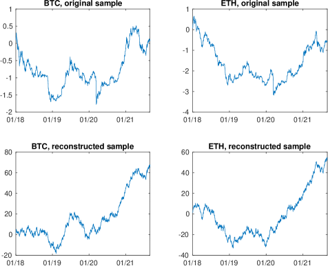
Figure 2: Log-price and pseudo log-price of cyptocurrencies

Table 7 gives the values of the test statistics. The PWY test does not identify explosive behavior in both prices, while the RVPWY test finds explosive behavior in the ETH series at the 10% level. Although the RVPWY test does not find explosive behavior in the BTC series, the test statistic is very close to the 10% critical value.

Table 7: Test statistics and $p$-values.

		PWY			RVPWY
BTC			$-0.780$			$1.069$
ETH			$0.848$			$1.282^{\ast}$

• Notes: Critical values are 2.094, 1.468 and 1.184 for the 1%, 5% and 10% significance level, respectively, for both tests. Rejection at these significance levels is denoted as ***, **, *, respectively.

We also plot the evolution of the RVDF detector and the DF detector in Figure 3, together with the critical values of the detector, which is -0.08, the 5% critical value of the DF distribution. This helps us better understanding the difference in the values of the RVDF and RVPWY statistics and the corresponding DF and PWY statistics. For the BTC series, the price decrease in the beginning the sample becomes less obvious in the reconstructed sample, such that the price increase in the latter sample becomes more pronounced. This explains why the RVDF detector crosses the $-0.08$ horizontal line after 2021, but the DF detector always stays below the line. However, the maximum of the RVDF detector (1.069 as in Table 7)) is still lower than the 10% critical value of the RVPWY test, such that we cannot conclude that explosive behavior exists in this series. For the ETH series, the DF detector identifies the downturn of the price as explosive behaviour, but fails to find explosive behavior during the time when the ETH price increases quickly from 2020. With the RVDF detector, we find results more in line with our intuition of the data: the downturn part shows less evidence of explosiveness, but the explosive behavior after 2021 can be detected now. The maximum of the RVDF detector (1.282 as in Table 7) is large enough to guarantee a rejection of the RVPWY test at 10% level now.

For the specific dates of the explosive regime, since the PWY test does not find any explosive behavior in both series and the RVPWY test only finds explosive behavior in the ETH series, we only report the starting date March 5, 2021 of the explosive behavior found by the RVDF detector. There are also a number of explosive regimes identified before March 5, 2021. However, the longest explosive regime found by the RVDF detector during the downturn of ETH price in 2018 was from October 12, 2018 to November 20, 2018. Since these durations are shorter than the smallest window we choose to calculate all the statistics, we do not report them.

6.2 Empirical bubble in monthly S&P500 index during the 1990s

The purpose of this empirical application is to illustrate how daily level stock index data can be exploited to estimate a monthly volatility measure, which can then be used in our methodology to help testing and date-stamping explosive behavior at the monthly frequency.

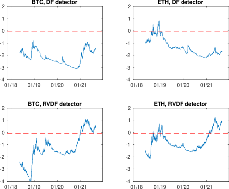
Figure 3: DF detector and RVDF detector

The dot-com bubble was a historic economic bubble and period of excessive speculation that occurred in the 1990s, a period of extreme growth in the usage and adaptation of the Internet by businesses and consumers. Phillips et al. (2011) studied the monthly real Nasdaq index, and Phillips et al. (2015a) studied the price-dividend ratio of S&P500 during the dot-com bubble, and both find explosive behavior. In this empirical application, we study the potential explosive behavior during this period in the nominal and real S&P500 indices using the proposed methodology, by exploiting the volatility information in the daily S&P500 price data, which is widely available but not used in the previous analysis. To study the explosive behavior in the nominal S&P500 index, our methodology can be applied directly. For the real S&P500 index, our realized volatility estimator cannot be applied because the Consumer Price Index (CPI) is not available at the daily level. We will first discuss an empirically meaningful approximation strategy for the monthly volatility of the real S&P500 index. Given the estimated volatility, we apply the testing and date-stamping methodology developed in this paper to the data, and compare the outcomes to those obtained by the PWY method. The sample period we use is January 1990 to June 2005, the same as in Phillips et al. (2011). The daily level S&P500 index data has been downloaded from Yahoo Finance. The monthly US CPI data has been downloaded from the US Federal Reserve website. Since we are using daily S&P500 returns to estimate monthly volatility, it is necessary to account for the mean estimate, therefore the realized variance estimator we use in this example is based on demeaned daily S&P500 returns.

6.2.1 Monthly volatility of S&P500 index

We consider testing the explosiveness in both the nominal and the real S&P500 index at the monthly frequency. Using the daily nominal S&P500 index data, it is straightforward to estimate the monthly volatility in the nominal S&P500 series. However, for the monthly volatility of the real S&P500 index, the daily real S&P500 index is not available due to the unavailability of the daily CPI data. Here we introduce an approximation strategy, where the monthly volatility of the real S&P500 series can be approximated by the monthly volatility of the nominal S&P500.

Denote the nominal S&P500 index as $S_{t}$, and the corresponding CPI by $P_{t}$. Then the monthly real S&P500 index $X_{t}$ is defined as $X_{t}=S_{t}/P_{t}$, so the monthly real S&P500 log-return is $\Delta\log X_{t}=\Delta\log S_{t}-\Delta\log P_{t}$. Its variance is

$$\mathrm{Var}(\Delta X_{t})=\mathrm{Var}(\Delta\log S_{t})+\mathrm{Var}(\Delta\log P_{t})-2\mathrm{Cov}(\Delta\log S_{t},\Delta\log P_{t}).$$

Looking at the empirical data at the monthly frequency, we find that the CPI, which represents the price level for consumer goods and services, has much smaller variability than the the stock price index. This can be seen in the variance-covariance matrix of monthly nominal S&P500 returns and monthly CPI inflation, given in Table 8. From the table, we can see that at the monthly level, the CPI variance and the CPI-S&P500 covariance are about a factor 500 smaller than the S&P500 variance. This empirical observation motivates the use of the approximation $\mathrm{Var}(\Delta\log X_{t})\approx\mathrm{Var}(\Delta\log S_{t})$.

Table 8: Variance-covariance matrix of monthly nominal S&P500 return and monthly CPI inflation, both in percentage, January 1990 to June 2005.

	S&P500	CPI
S&P500	$\leavevmode\nobreak\ \leavevmode\nobreak\ 15.69$	$-0.03$
CPI	$-0.03$	$\leavevmode\nobreak\ \leavevmode\nobreak\ 0.03$

Using this approximation, the variance of the real index can be estimated by the realized variance using the daily nominal stock index data. Indeed, although CPI does have a nontrivial effect on the level of real stock index, its effect on the variance is negligible. Since the daily stock index data are widely available from 1970s, these data can be used to improve our understanding of the volatility structure also in the real index.

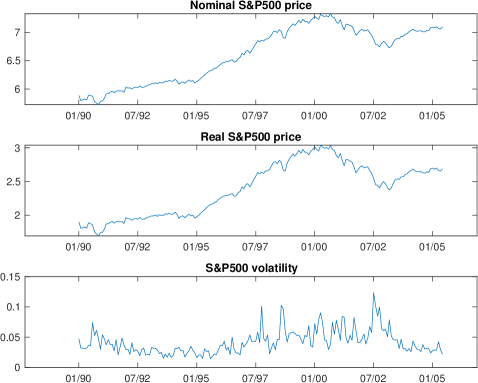
Figure 4: Monthly S&P500 series and volatility during the 1990s and early 2000s.

Applying the realized variance estimator, we estimate the monthly volatility of S&P500 from January 1990 to June 2005. The estimated realized volatility path, together with the plot of the nominal and the real S&P500 indices, is given in Figure 4. From the volatility estimate, the volatility seems in general higher during the bubble build-up period and obviously higher when the price drops.

We then apply the testing and date-stamping strategies developed in this paper to both the nominal and the real S&P500 series, and compare the result with those obtained by the PWY method. The results are summarized in Table 9. First, it seems that the RVPWY test gives slightly higher statistic values than the PWY test for both series, such that the RVPWY test rejects the null hypothesis at the 1% level in both the nominal and the real S&P500 series; while the PWY test also rejects the null hypothesis, but only at the 5% level in both series.

The results for date-stamping are also given in Figure 5. In the nominal series, the RVDF detector finds the explosive behavior from February 1995, 5 monthly earlier than the DF detector by PWY. In the real S&P500 series, the RVDF detector finds the explosive behavior from March 1995, which is 8 months earlier than PWY. For the conlusion time of the explosive regime, the nominal S&P500 index reaches its maximum in September 2000, and the corresponding real index peaked in April of the same year. In hindsight, it is reasonable to take the month when the series reached its maximum (i.e. when it started to crash) as the end of the bubble regime and hence, in the nominal series, the RVDF detector realizes the end of the bubble one month earlier than the DF detector; while in the real series, the DF detector finds the end of bubble one month earlier than the RVDF detector. Overall, it appears that the RVDF detector is more sensitive in detecting the start of a bubble; while the performance of the two detectors is similar in identifying the end of a bubble.

Table 9: Timeline of an explosive bubble in the S&P500 index.

	Nominal S&P500		Real S&P500
	RVPWY	PWY	RVPWY	PWY
Test statistic	2.2801	2.0071	2.3020	2.0015
Start of bubble	Feb 1995	Jul 1995	Mar 1995	Nov 1995
End of bubble	Jan 2001	Feb 2001	Jan 2001	Dec 2000
Monthly index maximum	Sep 2000		Apr 2000

7 Conclusion

In a new continuous-time framework, by incorporating the volatility information in data sampled at a higher frequency, we develop a powerful yet easy-to-implement test for the explosive behavior in data sampled at a lower frequency. The presence of stochastic volatility makes OLS estimation of the persistence parameter inefficient, and existing asymptotic null distributions of test statistics (derived under homoskedasticity) invalid. To achieve valid inference for the explosive behavior, we propose to devolatize the price series sampled at the lower frequency using realized volatility from data sampled at the higher frequency. We conduct simulation studies to compare the performance of our method relative to some existing methods. Simulation results suggest that our test has well-controlled size and using high-frequency volatility measures to devolatize data also brings efficiency improvement, in the sense that our test has markedly improved power performance than the existing methods. Empirical applications using the cryptocurrencies and the S&P500 prices allow us to find some interesting empirical results.

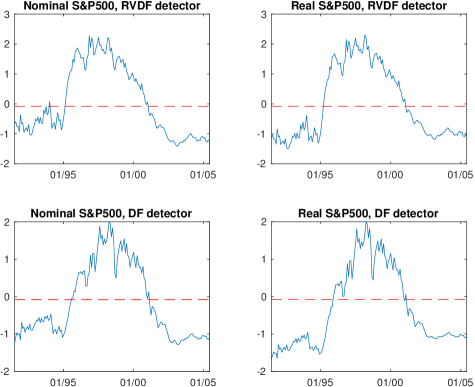
Figure 5: Date-stamping the explosive regime in the nominal and the real S&P500 index.

Appendix: Lemmas and Proof of Theorems

We first give lemmas to develop the asymptotic properties of the realized volatility estimator under the double asymptotics $h\rightarrow 0$ and $n\rightarrow\infty$, which will be used in the proof of the main theorems. Notice that these results go beyond most of the existing results on realized volatility, where an in-fill asymptotic scheme ($h\rightarrow 0$, $n$ fixed) is used.

In the proofs, $C$ denotes a generic positive constant number, the value of which may change from one equation to the next.

Lemma 1.

Under the same assumptions as in Theorem 1, letting

$$Z_{i,j}:=\left(\int_{t_{i-1,j-1}}^{t_{i-1,j}}\sigma_{u}\mathrm{d}W_{u}\right)^{2}-\int_{t_{i-1,j-1}}^{t_{i-1,j}}\sigma_{u}^{2}\mathrm{d}u,$$

we have

$$E\left(\sum_{j=1}^{M}Z_{i,j}\right)^{2}=O(h),\quad\forall i.$$

Proof.

By the property of stochastic integrals, and in particular Ito’s isometry, $EZ_{i,j}=0$, and $Z_{i,j}$ is a martingale difference sequence indexed by $j$ for every $i$. We have

$$E\left(\sum_{j=1}^{M}Z_{i,j}\right)^{2} \leqslant C\times E\left(\sum_{j=1}^{M}Z_{i,j}^{2}\right)$$ (A.1)

$$= C\times E\sum_{j=1}^{M}\left(\left(\int_{t_{i-1,j-1}}^{t_{i-1,j}}\sigma_{u}\mathrm{d}W_{u}\right)^{2}-\int_{t_{i-1,j-1}}^{t_{i-1,j}}\sigma_{u}^{2}\mathrm{d}u\right)^{2}$$

$$\leqslant 2C\times E\sum_{j=1}^{M}\left(\left(\int_{t_{i-1,j-1}}^{t_{i-1,j}}\sigma_{u}\mathrm{d}W_{u}\right)^{4}+\left(\int_{t_{i-1,j-1}}^{t_{i-1,j}}\sigma_{u}^{2}\mathrm{d}u\right)^{2}\right),$$

where we use the Burkholder’s inequality for the $L_{2}$ norm (cf. Shiryaev (1995), p. 499) for the martingale difference sequence in the first step; in the last step we use the generic inequality $(a+b)^{2}\leqslant 2a^{2}+2b^{2}$ for any real numbers $a$ and $b$. Now, by the Burkholder-Davis-Gundy inequality, for all $i,j$,

$$E\left(\int_{t_{i-1,j-1}}^{t_{i-1,j}}\sigma_{u}\mathrm{d}W_{u}\right)^{4} \leqslant CE\left(\int_{t_{i-1,j-1}}^{t_{i-1,j}}\sigma_{u}^{2}\mathrm{d}u\right)^{2}=O(h^{2}),$$

by the uniform boundedness of the volatility process. For the same reason, the second term in the brackets in (A.1) also satisfies that, for all $i,j$,

$$E\left(\int_{t_{i-1,j-1}}^{t_{i-1,j}}\sigma_{u}^{2}\mathrm{d}u\right)^{2}=O(h^{2}).$$

Continuing on (A.1), we have

$$E\left(\sum_{j=1}^{M}Z_{i,j}\right)^{2}=O(h^{2}M)=O(h),\quad\forall i,$$

which completes the proof. ∎

Lemma 2.

Under the same assumptions as in Theorem 1,

$$\max_{1\leqslant i\leqslant n}|\hat{\omega}_{i}^{2}-\omega_{i}^{2}|=O_{p}\left(\sqrt{nh}\right).$$

Proof.

Under the assumptions, we have

$$\hat{\omega}_{i}^{2}-\omega_{i}^{2}=\sum_{j=1}^{M}Z_{i,j},\quad\forall i,$$

using the notation $Z_{i,j}$ defined in Lemma 1. Therefore, for any $\eta>0$,

$$P\left(\max_{1\leqslant i\leqslant n}|\hat{\omega}_{i}^{2}-\omega_{i}^{2}|\geqslant\eta\sqrt{hn}\right) = P\left(\max_{1\leqslant i\leqslant n}\left|\sum_{j=1}^{M}Z_{i,j}\right|\geqslant\eta\sqrt{hn}\right)$$

$$\leqslant \sum_{i=1}^{n}P\left(\left|\sum_{j=1}^{M}Z_{i,j}\right|\geqslant\eta\sqrt{hn}\right)$$

$$\leqslant \sum_{i=1}^{n}E\left|\sum_{j=1}^{M}Z_{i,j}\right|^{2}/(\eta^{2}hn),$$

where the Markov inequality is used in the third step. Using Lemma 1, we have

$$P\left(\max_{1\leqslant i\leqslant n}|\hat{\omega}_{i}^{2}-\omega_{i}^{2}|\geqslant\eta\sqrt{hn}\right)=O(1),$$

and the claim of the lemma follows. ∎

Lemma 3.

If the time-varying mean-reversion parameter $\kappa_{t}$ satisfies

$$\kappa_{t}=\left\{\begin{array}[]{ll}0,&t\leqslant t_{\lfloor\tau_{1}n\rfloor}\\ \kappa,&t_{\lfloor\tau_{1}n\rfloor}<t\leqslant t_{\lfloor\tau_{2}n\rfloor},\\ 0,&t_{i}>t_{\lfloor\tau_{2}n\rfloor,}\end{array}\right.$$

the solution of the model is

$$y_{t}=\left\{\begin{array}[]{ll}\int_{0}^{t}\sigma_{u}\mathrm{d}W_{u}&t\leqslant t_{\lfloor\tau_{1}n\rfloor},\\ y_{t_{\lfloor\tau_{1}n\rfloor}}e^{\kappa(t-t_{\lfloor\tau_{1}n\rfloor})}+e^{\kappa t}\int_{t_{\lfloor\tau_{1}n\rfloor}}^{t}\sigma_{u}e^{-\kappa u}\mathrm{d}W_{u}&t_{\lfloor\tau_{1}n\rfloor}<t\leqslant t_{\lfloor\tau_{2}n\rfloor},\\ y_{t_{\lfloor\tau_{2}n\rfloor}}+\int_{t_{\lfloor\tau_{2}n\rfloor}}^{t}\sigma_{u}\mathrm{d}W_{u}&t>t_{\lfloor\tau_{2}n\rfloor}.\end{array}\right.$$

Proof.

First notice that for the constant mean-reversion parameter model given by

$$\mathrm{d}y_{t}=\kappa y_{t}\mathrm{d}t+\sigma_{t}\mathrm{d}W_{t},$$

the solution is:

$$y_{t}=y_{0}e^{\kappa t}+e^{\kappa t}\int_{0}^{t}\sigma_{u}e^{-\kappa u}\mathrm{d}W_{u}.$$

When $t\leqslant t_{\lfloor\tau_{1}n\rfloor}$ or $t>t_{\lfloor\tau_{2}n\rfloor}$, the process has a constant time-varying parameter $\kappa=0$, and the process starts from $y_{0}=0$ and $y_{t_{\lfloor\tau_{2}n\rfloor}}$ respectively. So the claimed solution in these two regimes follow easily.

When $t_{\lfloor\tau_{1}n\rfloor}<t\leqslant t_{\lfloor\tau_{2}n\rfloor}$, the process has a constant time-varying parameter $\kappa>0$, and the process starts from the last point of the previous unit regime $y_{\lfloor\tau_{1}n\rfloor}=\int_{0}^{\lfloor\tau_{1}n\rfloor}\sigma_{u}\mathrm{d}W_{u}$. It is straightforward to check that the solution in this regime is

$$y_{t}=y_{t_{\lfloor\tau_{1}n\rfloor}}e^{\kappa(t-t_{\lfloor\tau_{1}n\rfloor})}+e^{\kappa t}\int_{t_{\lfloor\tau_{1}n\rfloor}}^{t}\sigma_{u}e^{-\kappa u}\mathrm{d}W_{u}.$$

Then the proof of the lemma is finished. ∎

From the result of the above lemma, we can see that in the unit root regime, the order of the process is $n^{1/2}$. When $\kappa=c/n^{\alpha}$ for some $c>0$ and $0<\alpha<1$, i.e., the process is mildly explosive, the process is dominated by the initial value of the regime. This fact can be seen by noticing that the solution of this regime takes the form $y_{t_{\lfloor\tau_{1}n\rfloor}}e^{\kappa(t-t_{\lfloor\tau_{1}n\rfloor})}+e^{\kappa(t-t_{\lfloor\tau_{1}n\rfloor})}\int_{t_{\lfloor\tau_{1}n\rfloor}}^{t}\sigma_{u}e^{-\kappa(u-t_{\lfloor\tau_{1}n\rfloor})}\mathrm{d}W_{u}$. In the first term, $y_{t_{\lfloor\tau_{1}n\rfloor}}$ has order $n^{1/2}$; while in the second term, the order of the $\int_{t_{\lfloor\tau_{1}n\rfloor}}^{t}\sigma_{u}e^{-\kappa(u-t_{\lfloor\tau_{1}n\rfloor})}\mathrm{d}W_{u}$ term is smaller. This is because, by Ito’s isometry,

$$E\left(\int_{t_{\lfloor\tau_{1}n\rfloor}}^{t}\sigma_{u}e^{-\kappa(u-t_{\lfloor\tau_{1}n\rfloor})}\mathrm{d}W_{u}\right)^{2} = \int_{t_{\lfloor\tau_{1}n\rfloor}}^{t}E\sigma_{u}^{2}e^{-2\kappa(u-t_{\lfloor\tau_{1}n\rfloor})}\mathrm{d}u$$

$$\leqslant C\int_{t_{\lfloor\tau_{1}n\rfloor}}^{t}e^{-2\kappa(u-t_{\lfloor\tau_{1}n\rfloor})}\mathrm{d}u$$

$$= -C\frac{1}{2\kappa}\left(e^{-2\kappa(t-t_{\lfloor\tau_{1}n\rfloor})}-1\right).$$

When $t-t_{\lfloor\tau_{1}n\rfloor}$ is finite, $\kappa(t-t_{\lfloor\tau_{1}n\rfloor})$ has order $\kappa$ as $\kappa\rightarrow 0$, and the final right-hand side expression in the previous equation can be expanded as

$$-C\frac{1}{2\kappa}\left(-2\kappa(t-t_{\lfloor\tau_{1}n\rfloor})+\frac{1}{2}(-2\kappa(t-t_{\lfloor\tau_{1}n\rfloor}))^{2}+\cdots\right)=O(1).$$

When $t=t_{\lfloor\tau n\rfloor}$ for some $\tau>\tau_{1}$, $t-t_{\lfloor\tau_{1}n\rfloor}=(\lfloor\tau n\rfloor-\lfloor\tau_{1}n\rfloor)H=O(n)$ and it follows that $-2\kappa(t-t_{\lfloor\tau_{1}n\rfloor})\sim-2n^{1-\alpha}\rightarrow-\infty$ and therefore $e^{-2\kappa(t-t_{\lfloor\tau_{1}n\rfloor})}-1\rightarrow-1$. We then have

$$-C\frac{1}{2\kappa}\left(e^{-2\kappa(t-t_{\lfloor\tau_{1}n\rfloor})}-1\right)\sim\frac{1}{2\kappa}=O(n^{\alpha})=o(n),$$

and $\int_{t_{\lfloor\tau_{1}n\rfloor}}^{t}\sigma_{u}e^{-\kappa(u-t_{\lfloor\tau_{1}n\rfloor})}\mathrm{d}W_{u}=o_{p}(n^{1/2})$. In either case, the $\int_{t_{\lfloor\tau_{1}n\rfloor}}^{t}\sigma_{u}e^{-\kappa(u-t_{\lfloor\tau_{1}n\rfloor})}\mathrm{d}W_{u}$ term is dominated by the $y_{t_{\lfloor\tau_{1}n\rfloor}}$ term, which is $O_{p}(n^{1/2})$.

Lemma 4.

Under the same assumptions as in Theorem 4,

$$\max_{1\leqslant i\leqslant n}|\hat{\omega}_{i}^{2}-\omega_{i}^{2}|=O_{p}\left(n^{1-2\alpha}e^{2c/n^{\alpha}H(\lfloor\tau_{2}n\rfloor-\lfloor\tau_{1}n\rfloor)}h\vee\sqrt{nh}\right)=o_{p}(1),$$

where $\vee$ means the maximum.

Proof.

Under the same assumptions as in Theorem 4 and the alternative model, we have

$$\hat{\omega}_{i}^{2}-\omega_{i}^{2}=\sum_{j=1}^{M}\kappa_{t}^{2}\left(\int_{t_{i-1,j-1}}^{t_{i-1,j}}y_{u}\mathrm{d}u\right)^{2}+\sum_{j=1}^{M}\kappa_{t}\left(\int_{t_{i-1,j-1}}^{t_{i-1,j}}y_{u}\mathrm{d}u\right)\left(\int_{t_{i-1,j-1}}^{t_{i-1,j}}\sigma_{u}\mathrm{d}W_{u}\right)+\sum_{j=1}^{M}Z_{i,j},$$

using the notation $Z_{i,j}$ defined in Lemma 1. The value of $\kappa_{t}$ depends on which of the three regimes $y_{t_{i}}$ is in. When $t_{i}\leqslant t_{i_{1}}$ or $t_{i}>t_{i_{2},}$ $\kappa_{t}=0$ and using the proof of Lemma 2, we have

$$\max_{1\leqslant i\leqslant i_{1},i_{2}<i\leqslant n}|\hat{\omega}_{i}^{2}-\omega_{i}^{2}|=O_{p}\left(\sqrt{nh}\right).$$ (A.2)

When $t_{i_{1}}<t_{i}\leqslant t_{i_{2}}$, i.e., in the explosive regime, $\kappa_{t}=\kappa=c/n^{\alpha}$, so that

$$\hat{\omega}_{i}^{2}-\omega_{i}^{2}$$

$$= \sum_{j=1}^{M}\kappa^{2}\left(\int_{t_{i-1,j-1}}^{t_{i-1,j}}y_{u}\mathrm{d}u\right)^{2}+\sum_{j=1}^{M}\kappa\left(\int_{t_{i-1,j-1}}^{t_{i-1,j}}y_{u}\mathrm{d}u\right)\left(\int_{t_{i-1,j-1}}^{t_{i-1,j}}\sigma_{u}\mathrm{d}W_{u}\right)+\sum_{j=1}^{M}Z_{i,j}$$

$$=: A+B+C.$$

We now examine each term separately. For term $A$, using the solution in Lemma 3,

$$\max_{i_{1}<i\leqslant i_{2}}|A| = \max_{i_{1}<i\leqslant i_{2}}\kappa^{2}\sum_{j=1}^{M}\left(\int_{t_{i-1,j-1}}^{t_{i-1,j}}y_{u}\mathrm{d}u\right)^{2}$$

$$= \max_{i_{1}<i\leqslant i_{2}}\kappa^{2}\sum_{j=1}^{M}\left(\int_{t_{i-1,j-1}}^{t_{i-1,j}}y_{t_{\lfloor\tau_{1}n\rfloor}}e^{\kappa(u-t_{\lfloor\tau_{1}n\rfloor})}\mathrm{d}u(1+o_{p}(1))\right)^{2}$$

$$= \max_{i_{1}<i\leqslant i_{2}}\sum_{j=1}^{M}\left(y_{t_{\lfloor\tau_{1}n\rfloor}}e^{\kappa(t_{i-1,j-1}-t_{\lfloor\tau_{1}n\rfloor})}(e^{\kappa(t_{i-1,j}-t_{i-1,j-1})}-1)(1+o_{p}(1))\right)^{2}$$

$$= y_{t_{\lfloor\tau_{1}n\rfloor}}^{2}(e^{\kappa h}-1)^{2}e^{-2\kappa t_{\lfloor\tau_{1}n\rfloor}}\max_{i_{1}<i\leqslant i_{2}}\sum_{j=1}^{M}e^{2\kappa t_{i-1,j-1}}(1+o_{p}(1))$$

$$= y_{t_{\lfloor\tau_{1}n\rfloor}}^{2}(e^{\kappa h}-1)^{2}e^{-2\kappa t_{\lfloor\tau_{1}n\rfloor}}\max_{i_{1}<i\leqslant i_{2}}h^{-1}\int_{t_{i-1}}^{t_{i}}e^{2\kappa u}\mathrm{d}u(1+o_{p}(1))$$

$$= y_{t_{\lfloor\tau_{1}n\rfloor}}^{2}(e^{\kappa h}-1)^{2}e^{-2\kappa t_{\lfloor\tau_{1}n\rfloor}}\max_{i_{1}<i\leqslant i_{2}}(2\kappa h)^{-1}e^{2\kappa t_{i}}(1-e^{-2\kappa H})$$

$$= y_{t_{\lfloor\tau_{1}n\rfloor}}^{2}(e^{\kappa h}-1)^{2}e^{-2\kappa t_{\lfloor\tau_{1}n\rfloor}}(2\kappa h)^{-1}e^{2\kappa\lfloor\tau_{2}n\rfloor}(1-e^{-2\kappa H})$$

$$= O_{p}(n^{1-2\alpha}e^{2c/n^{\alpha}H(\lfloor\tau_{2}n\rfloor-\lfloor\tau_{1}n\rfloor)}h).$$

Using the same proof as for term $A$, we have

$$\max_{i_{1}<i\leqslant i_{2}}|C|=O_{p}\left(\sqrt{nh}\right).$$

By the Cauchy-Schwarz inequality, the cross product term $B$ cannot be larger than both $A$ and $C$. Therefore, we have

$$\max_{i_{1}<i\leqslant i_{2}}|\hat{\omega}_{i}^{2}-\omega_{i}^{2}|=O_{p}(n^{1-2\alpha}e^{2c/n^{\alpha}H(\lfloor\tau_{2}n\rfloor-\lfloor\tau_{1}n\rfloor)}h\vee\sqrt{nh}).$$

Hence,

$$\max_{1\leqslant i\leqslant n}|\hat{\omega}_{i}^{2}-\omega_{i}^{2}|=O_{p}\left(n^{1-2\alpha}e^{2c/n^{\alpha}H(\lfloor\tau_{2}n\rfloor-\lfloor\tau_{1}n\rfloor)}h\vee\sqrt{nh}\right),$$

which is $o_{p}(1)$ under Assumption A2 and A3. ∎

Lemma 5.

Under either the assumptions as in Theorem 1 or as in Theorem 4, $\max_{1\leqslant i\leqslant n}|\omega_{i}^{-1}|=O_{p}(1)$ and $\max_{1\leqslant i\leqslant n}|\hat{\omega}_{i}^{-1}|=O_{p}(1)$.

Proof.

We first prove the result under the same assumptions as in Theorem 1. It is clear that $\max_{1\leqslant i\leqslant n}|\omega_{i}^{-1}|=O_{p}(1)$ is a consequence of the strict positiveness of $\sigma$ in Assumption A1. For the realized variance $\hat{\omega}_{i}^{2}$, first notice that

$$\min_{1\leqslant i\leqslant n}|\omega_{i}^{2}|\leqslant\min_{1\leqslant i\leqslant n}|\hat{\omega}_{i}^{2}|+\min_{1\leqslant i\leqslant n}|\omega_{i}^{2}-\hat{\omega}_{i}^{2}|\leqslant\min_{1\leqslant i\leqslant n}|\hat{\omega}_{i}^{2}|+\max_{1\leqslant i\leqslant n}|\omega_{i}^{2}-\hat{\omega}_{i}^{2}|,$$

which implies that

$$\min_{1\leqslant i\leqslant n}|\hat{\omega}_{i}^{2}| \geqslant \min_{1\leqslant i\leqslant n}|\omega_{i}^{2}|-\max_{1\leqslant i\leqslant n}|\omega_{i}^{2}-\hat{\omega}_{i}^{2}|.$$

Again by Assumption A1, $\min_{1\leqslant i\leqslant n}\omega_{i}^{2}>c$; together with the result of Lemma 2 we have $\min_{1\leqslant i\leqslant n}|\hat{\omega}_{i}^{2}|\geqslant c+o_{p}(1)$ for a positive constant $c$, and therefore we have $\max_{1\leqslant i\leqslant n}|\hat{\omega}_{i}^{-2}|=O_{p}(1)$, and the second claim of the lemma is proved.

The results under the same assumptions as in Theorem 4 can be proved in the same way. Using the uniform consistency result in Lemma 4, all the above arguments go through. ∎

Lemma 6.

Under the same assumptions as in Theorem 4, for $i$ such that $t_{\lfloor\tau_{1}n\rfloor}<t_{i}\leqslant t_{\lfloor\tau_{2}n\rfloor}$,

$$\Delta x_{i}=\frac{y_{t_{i}}-y_{t_{i-1}}}{\hat{\omega}_{i}}=\frac{\kappa\int_{t_{i-1}}^{t_{i}}y_{u}\mathrm{d}u}{\omega_{i}}(1+o_{p}(1))=O_{p}\left(n^{1/2-\alpha}e^{\kappa(t_{i-1}-t_{\lfloor\tau_{1}n\rfloor})}\right).$$

Proof.

By definition

$$\Delta x_{i}=\frac{y_{t_{i}}-y_{t_{i-1}}}{\hat{\omega}_{i}}=\frac{\kappa\int_{t_{i-1}}^{t_{i}}y_{u}\mathrm{d}u}{\hat{\omega}_{i}}+\frac{\omega_{i}}{\hat{\omega}_{i}}\varepsilon_{i}=\frac{\kappa\int_{t_{i-1}}^{t_{i}}y_{u}\mathrm{d}u}{\omega_{i}}+\kappa\left(\frac{\int_{t_{i-1}}^{t_{i}}y_{u}\mathrm{d}u}{\hat{\omega}_{i}}-\frac{\int_{t_{i-1}}^{t_{i}}y_{u}\mathrm{d}u}{\omega_{i}}\right)+\frac{\omega_{i}}{\hat{\omega}_{i}}\varepsilon_{i}.$$

In the following we derive that

$$\frac{\int_{t_{i-1}}^{t_{i}}y_{u}\mathrm{d}u}{\omega_{i}} = O_{p}\left(n^{1/2}e^{\kappa(t_{i-1}-t_{\lfloor\tau_{1}n\rfloor})}\right),$$

$$\left|\frac{\int_{t_{i-1}}^{t_{i}}y_{u}\mathrm{d}u}{\hat{\omega}_{i}}-\frac{\int_{t_{i-1}}^{t_{i}}y_{u}\mathrm{d}u}{\omega_{i}}\right| = o_{p}\left(\frac{\int_{t_{i-1}}^{t_{i}}y_{u}\mathrm{d}u}{\omega_{i}}\right),$$

$$\frac{\omega_{i}}{\hat{\omega}_{i}}\varepsilon_{i} = O_{p}(1).$$

Then the claim of the Lemma follows.

First, using the dominating part of the solution of the continuous-time process in the explosive regime as derived in Lemma 3, we have

$$\frac{\int_{t_{i-1}}^{t_{i}}y_{u}\mathrm{d}u}{\omega_{i}} = \frac{\int_{t_{i-1}}^{t_{i}}\left(y_{t_{\lfloor\tau_{1}n\rfloor}}e^{\kappa(u-t_{\lfloor\tau_{1}n\rfloor})}\right)\mathrm{d}u(1+o_{p}(1))}{\omega_{i}}$$

$$= \frac{y_{t_{\lfloor\tau_{1}n\rfloor}}e^{-\kappa t_{\lfloor\tau_{1}n\rfloor}}}{\omega_{i}}\int_{t_{i-1}}^{t_{i}}e^{\kappa u}\mathrm{d}u(1+o_{p}(1))$$

$$= \frac{y_{t_{\lfloor\tau_{1}n\rfloor}}e^{-\kappa t_{\lfloor\tau_{1}n\rfloor}}}{\omega_{i}\kappa}e^{\kappa t_{i-1}}(e^{\kappa(t_{i}-t_{i-1})}-1)(1+o_{p}(1))$$

$$= O_{p}\left(n^{1/2}e^{\kappa(t_{i-1}-t_{\lfloor\tau_{1}n\rfloor})}\right).$$

Next,

$$\left|\frac{\int_{t_{i-1}}^{t_{i}}y_{u}\mathrm{d}u}{\hat{\omega}_{i}}-\frac{\int_{t_{i-1}}^{t_{i}}y_{u}\mathrm{d}u}{\omega_{i}}\right|\leqslant\left|\int_{t_{i-1}}^{t_{i}}y_{u}\mathrm{d}u\right|\left|\frac{1}{\hat{\omega}_{i}\omega_{i}}\right||\hat{\omega}_{i}-\omega_{i}|=o_{p}\left(\left|\frac{\int_{t_{i-1}}^{t_{i}}y_{u}\mathrm{d}u}{\omega_{i}}\right|\right),$$

using Lemma 4. Finally, $\frac{\omega_{i}}{\hat{\omega}_{i}}\varepsilon_{i}=O_{p}(1)$ is an obvious consequence of Lemma 4 and the proof for the lemma is completed. ∎

Lemma 7.

Under the same assumptions as in Theorem 4, for $i$ such that $t_{\lfloor\tau_{1}n\rfloor}<t_{i}\leqslant t_{\lfloor\tau_{2}n\rfloor}$,

$$\sum_{i=\lfloor\tau_{1}n\rfloor+1}^{\lfloor\tau n\rfloor}\Delta x_{i}=\sum_{i=\lfloor\tau_{1}n\rfloor+1}^{\lfloor\tau n\rfloor}\frac{\kappa\int_{t_{i-1}}^{t_{i}}y_{u}\mathrm{d}u}{\omega_{i}}(1+o_{p}(1))=O_{p}(n^{1/2}e^{\kappa H(\lfloor\tau n\rfloor-\lfloor\tau_{1}n\rfloor)}).$$

Proof.

By definition, we have

$$\sum_{i=\lfloor\tau_{1}n\rfloor+1}^{\lfloor\tau n\rfloor}\Delta x_{i} = \sum_{i=\lfloor\tau_{1}n\rfloor+1}^{\lfloor\tau n\rfloor}\frac{\kappa\int_{t_{i-1}}^{t_{i}}y_{u}\mathrm{d}u}{\hat{\omega}_{i}}+\sum_{i=\lfloor\tau_{1}n\rfloor+1}^{\lfloor\tau n\rfloor}\frac{\omega_{i}}{\hat{\omega}_{i}}\varepsilon_{i}$$

$$= \sum_{i=\lfloor\tau_{1}n\rfloor+1}^{\lfloor\tau n\rfloor}\frac{\kappa\int_{t_{i-1}}^{t_{i}}y_{u}\mathrm{d}u}{\omega_{i}}+\sum_{i=\lfloor\tau_{1}n\rfloor+1}^{\lfloor\tau n\rfloor}\kappa\left(\frac{\int_{t_{i-1}}^{t_{i}}y_{u}\mathrm{d}u}{\hat{\omega}_{i}}-\frac{\int_{t_{i-1}}^{t_{i}}y_{u}\mathrm{d}u}{\omega_{i}}\right)+\sum_{i=\lfloor\tau_{1}n\rfloor+1}^{\lfloor\tau n\rfloor}\frac{\omega_{i}}{\hat{\omega}_{i}}\varepsilon_{i}$$

In the following, we derive that

$$\sum_{i=\lfloor\tau_{1}n\rfloor+1}^{\lfloor\tau n\rfloor}\frac{\int_{t_{i-1}}^{t_{i}}y_{u}\mathrm{d}u}{\omega_{i}} = O_{p}(n^{\alpha+1/2}e^{\kappa H(\lfloor\tau n\rfloor-\lfloor\tau_{1}n\rfloor)}),$$

$$\left|\sum_{i=\lfloor\tau_{1}n\rfloor+1}^{\lfloor\tau n\rfloor}\left(\frac{\int_{t_{i-1}}^{t_{i}}y_{u}\mathrm{d}u}{\hat{\omega}_{i}}-\frac{\int_{t_{i-1}}^{t_{i}}y_{u}\mathrm{d}u}{\omega_{i}}\right)\right| = o_{p}\left(\sum_{i=\lfloor\tau_{1}n\rfloor+1}^{\lfloor\tau n\rfloor}\frac{\int_{t_{i-1}}^{t_{i}}y_{u}\mathrm{d}u}{\omega_{i}}\right),$$

$$\sum_{i=\lfloor\tau_{1}n\rfloor+1}^{\lfloor\tau n\rfloor}\frac{\omega_{i}}{\hat{\omega}_{i}}\varepsilon_{i} = O_{p}(n^{1/2}),$$

The claim of the Lemma follows.

First, using the dominating part of the solution of the process in the explosive regime as derived in Lemma 3, we have

$$\sum_{i=\lfloor\tau_{1}n\rfloor+1}^{\lfloor\tau n\rfloor}\frac{\int_{t_{i-1}}^{t_{i}}y_{u}\mathrm{d}u}{\omega_{i}} = \sum_{i=\lfloor\tau_{1}n\rfloor+1}^{\lfloor\tau n\rfloor}\frac{\int_{t_{i-1}}^{t_{i}}\left(y_{t_{\lfloor\tau_{1}n\rfloor}}e^{\kappa(u-t_{\lfloor\tau_{1}n\rfloor})}\right)\mathrm{d}u}{\omega_{i}}$$

$$= \sum_{i=\lfloor\tau_{1}n\rfloor+1}^{\lfloor\tau n\rfloor}\frac{y_{t_{\lfloor\tau_{1}n\rfloor}}e^{-t_{\lfloor\tau_{1}n\rfloor}}}{\omega_{i}\kappa}e^{\kappa t_{i-1}}(e^{\kappa(t_{i}-t_{i-1})}-1)$$

$$= y_{t_{\lfloor\tau_{1}n\rfloor}}\sum_{i=\lfloor\tau_{1}n\rfloor+1}^{\lfloor\tau n\rfloor}\frac{1}{\omega_{i}}e^{\kappa(t_{i-1}-t_{\lfloor\tau_{1}n\rfloor})}$$

$$= y_{t_{\lfloor\tau_{1}n\rfloor}}O\left(\sum_{i=\lfloor\tau_{1}n\rfloor+1}^{\lfloor\tau n\rfloor}e^{\kappa(t_{i-1}-t_{\lfloor\tau_{1}n\rfloor})}\right)$$

$$= y_{t_{\lfloor\tau_{1}n\rfloor}}O\left(\frac{1-e^{\kappa H(\lfloor\tau n\rfloor-\lfloor\tau_{1}n\rfloor)}}{1-e^{\kappa H}}\right)$$

$$= O_{p}(n^{\alpha+1/2}e^{\kappa H(\lfloor\tau n\rfloor-\lfloor\tau_{1}n\rfloor)}).$$

Next,

$$\left|\sum_{i=\lfloor\tau_{1}n\rfloor+1}^{\lfloor\tau n\rfloor}\left(\frac{\int_{t_{i-1}}^{t_{i}}y_{u}\mathrm{d}u}{\hat{\omega}_{i}}-\frac{\int_{t_{i-1}}^{t_{i}}y_{u}\mathrm{d}u}{\omega_{i}}\right)\right| \leqslant \sum_{i=\lfloor\tau_{1}n\rfloor+1}^{\lfloor\tau n\rfloor}\left|\int_{t_{i-1}}^{t_{i}}y_{u}\mathrm{d}u\right|\frac{1}{|\hat{\omega}_{i}\omega_{i}|}|\hat{\omega}_{i}-\omega_{i}|$$

$$= o_{p}\left(\sum_{i=\lfloor\tau_{1}n\rfloor+1}^{\lfloor\tau n\rfloor}\left|\frac{\int_{t_{i-1}}^{t_{i}}y_{u}\mathrm{d}u}{\omega_{i}}\right|\right),$$

using the uniform consistency of the realized variance estimator in Lemma 4. Finally, $\sum_{i=\lfloor\tau_{1}n\rfloor+1}^{\lfloor\tau n\rfloor}\frac{\omega_{i}}{\hat{\omega}_{i}}\varepsilon_{i}=O_{p}(n^{1/2})$ can be shown in the same way as in the proof of Theorem 1 and the proof of the Lemma is completed. ∎

Proof.

(of Theorem 1) Under the null,

$$\frac{1}{\sqrt{n}}x_{[n{\tau}]} = \frac{1}{\sqrt{n}}\sum_{i=1}^{[n{\tau}]}\frac{y_{t_{i}}-y_{t_{i-1}}}{\hat{\omega}_{i}}$$

$$= \frac{1}{\sqrt{n}}\sum_{i=1}^{[n{\tau}]}\frac{\omega_{i}\varepsilon_{i}}{\hat{\omega}_{i}}$$

$$= \frac{1}{\sqrt{n}}\sum_{i=1}^{[n{\tau}]}\varepsilon_{i}+\frac{1}{\sqrt{n}}\sum_{i=1}^{[n{\tau}]}\left(\frac{\omega_{i}}{\hat{\omega}_{i}}-1\right)\varepsilon_{i}.$$

The first term converges to $B_{s}$. If the second term is $o_{p}(1)$, the claim of the theorem is proved. Now we show that the second term is $o_{p}(1)$.

For the second term

$$\left|\frac{1}{\sqrt{n}}\sum_{i=1}^{[n{\tau}]}\left(\frac{\omega_{i}}{\hat{\omega}_{i}}-1\right)\varepsilon_{i}\right|$$ (A.3)

$$= \left|\frac{1}{\sqrt{n}}\sum_{i=1}^{[n{\tau}]}(\omega_{i}-\hat{\omega}_{i})\varepsilon_{i}\omega_{i}^{-1}\right|$$

$$= \left|\frac{1}{\sqrt{n}}\sum_{i=1}^{[n{\tau}]}(\omega_{i}^{2}-\hat{\omega}_{i}^{2})\varepsilon_{i}\omega_{i}^{-1}(\omega_{i}+\hat{\omega}_{i})^{-1}\right|$$

$$\leqslant \max_{1\leqslant i\leqslant n}(\omega_{i}^{-1}(\omega_{i}+\hat{\omega}_{i})^{-1})\left|\frac{1}{\sqrt{n}}\sum_{i=1}^{[n{\tau}]}\varepsilon_{i}(\omega_{i}^{2}-\hat{\omega}_{i}^{2})\right|$$

$$\leqslant \max_{1\leqslant i\leqslant n}(\omega_{i}^{-1}(\omega_{i}+\hat{\omega}_{i})^{-1})\left(\frac{1}{n}\sum_{i=1}^{[n{\tau}]}\varepsilon_{i}^{2}\right)^{1/2}\left(\sum_{i=1}^{[n{\tau}]}(\omega_{i}^{2}-\hat{\omega}_{i}^{2})^{2}\right)^{1/2},$$

using the Cauchy-Schwarz inequality in the last step. Under the null, $\omega_{i}^{2}-\hat{\omega}_{i}^{2}=\sum_{j=1}^{M}Z_{i,j}$, using the notation defined in Lemma 1. Now using the results of Lemma 1, Lemma 5 and the fact that $\frac{1}{n}\sum_{t=1}^{[n{\tau}]}\varepsilon_{t}^{2}=O_{p}(1)$, we have the above is of order $O_{p}(nh)$. Under the imposed assumption $nh\rightarrow 0$ we have thus shown that

$$\left|\frac{1}{\sqrt{n}}\sum_{i=1}^{[n{\tau}]}\left(\frac{\omega_{i}}{\hat{\omega}_{i}}-1\right)\varepsilon_{t}\right|=o_{p}(1).$$

This completes the proof.

∎

Proof.

(of Theorem 2) In view of the proof of Theorem 1, we have

$$\operatorname{RVDF}_{\tau}\Rightarrow\frac{\int_{0}^{\tau}B_{t}\mathrm{d}B_{t}}{\left(\int_{0}^{\tau}B_{t}^{2}\mathrm{d}t\right)^{1/2}},$$

where the weak convergence holds for the process $\operatorname{RVDF}_{\tau}$ indexed by $\tau$. Applying the argument in Phillips et al. (2011) for the supremum taken over the index $\tau$, the claimed result of this theorem follows. ∎

Proof.

(of Theorem 3) This is an easy consequence of Theorem 2 so we omit the details. ∎

Proof.

(of Theorem 4) The “with constant” version of the RVDF statistic defined for the sample $\{x_{s}\}_{s=0}^{\lfloor\tau n\rfloor}$ is

$$\operatorname{RVDF}_{\tau}:=\frac{\sum_{s=2}^{\lfloor\tau n\rfloor}\Delta\tilde{x}_{s}\tilde{x}_{s-1}}{\left(\sum_{s=2}^{\lfloor\tau n\rfloor}(\tilde{x}_{s-1})^{2}\right)^{1/2}(\hat{\sigma}_{\tau}^{2})^{1/2}},$$

where

$$\sum_{s=2}^{\lfloor\tau n\rfloor}\Delta\tilde{x}_{s}\tilde{x}_{s-1}=\sum_{s=2}^{\lfloor\tau n\rfloor}\Delta x_{s}x_{s-1}-\frac{1}{\lfloor\tau n\rfloor}(x_{\lfloor\tau n\rfloor}-x_{1})\left(\sum_{s=2}^{\lfloor\tau n\rfloor}x_{s-1}\right),$$ (A.4)

$$\sum_{s=2}^{\lfloor\tau n\rfloor}(\tilde{x}_{s-1})^{2}=\sum_{s=2}^{\lfloor\tau n\rfloor}(x_{s-1})^{2}-\frac{1}{\lfloor\tau n\rfloor}\left(\sum_{s=2}^{\lfloor\tau n\rfloor}x_{s-1}\right)^{2},$$ (A.5)

$$\hat{\sigma}_{\tau}^{2}=\frac{1}{\lfloor\tau n\rfloor-1}\sum_{s=2}^{\lfloor\tau n\rfloor}\left(\Delta\tilde{x}_{s}-\frac{\sum_{s=2}^{\lfloor\tau n\rfloor}\Delta\tilde{x}_{s}\tilde{x}_{s-1}}{\sum_{s=2}^{\lfloor\tau n\rfloor}(\tilde{x}_{s-1})^{2}}\tilde{x}_{s-1}\right)^{2}.$$ (A.6)

In the following, we will show

$$\left\{\begin{array}[]{ll}\operatorname{RVDF}_{\tau}=O_{p}(1),&\tau_{0}<\tau\leqslant\tau_{1},\\ \operatorname{RVDF}_{\tau}=O_{p}(n^{1/2}),&\tau_{1}<\tau\leqslant\tau_{2},\\ \operatorname{RVDF}_{\tau}=O_{p}(n^{1/2-\alpha/2}),&\tau_{2}<\tau\leqslant 1.\end{array}\right.$$

Applying the arguments in Phillips and Yu (2009a) and Phillips and Shi (2018), the claimed consistency result for the estimator of the start and end dates of the bubble follows. We now derive the above order results under the three regimes.

1) $\operatorname{RVDF}_{\tau}=O_{p}(1)$ for $\tau_{0}<\tau\leqslant\tau_{1}$.

This can be shown in the same way as the proof of Theorem 2.

2) $\operatorname{RVDF}_{\tau}=O_{p}(n^{1/2})$ for $\tau_{1}<\tau\leqslant\tau_{2}$.

We first examine the behavior of the numerator $\sum_{s=2}^{\lfloor\tau n\rfloor}\Delta\tilde{x}_{s}\tilde{x}_{s-1}$ when $\tau_{1}<\tau\leqslant\tau_{2}$. We examine each part of the expansion (A.4) separately. For the term $\sum_{s=2}^{\lfloor\tau n\rfloor}\Delta x_{s}x_{s-1}$, notice that

$$\sum_{s=2}^{\lfloor\tau n\rfloor}\Delta x_{s}x_{s-1} = \sum_{s=2}^{\lfloor\tau_{1}n\rfloor}\Delta x_{s}x_{s-1}+\sum_{s=\lfloor\tau_{1}n\rfloor+1}^{\lfloor\tau n\rfloor}\Delta x_{s}x_{s-1}$$

$$= \left(\sum_{s=\lfloor\tau_{1}n\rfloor+1}^{\lfloor\tau n\rfloor}\Delta x_{s}x_{s-1}\right)(1+o_{p}(1)).$$

Now, using Lemma 6, we have

$$\sum_{s=\lfloor\tau_{1}n\rfloor+1}^{\lfloor\tau n\rfloor}\Delta x_{s}x_{s-1}$$

$$= \left(\sum_{s=\lfloor\tau_{1}n\rfloor+1}^{\lfloor\tau n\rfloor}\left(\frac{\kappa\int_{t_{s-1}}^{t_{s}}y_{u}\mathrm{d}u}{\omega_{s}}\right)\left(\frac{\kappa\int_{t_{s-2}}^{t_{s-1}}y_{u}\mathrm{d}u}{\omega_{s-1}}+\cdots+\frac{\kappa\int_{t_{\lfloor\tau_{1}n\rfloor}}^{t_{\lfloor\tau_{1}n\rfloor+1}}y_{u}\mathrm{d}u}{\omega_{\lfloor\tau_{1}n\rfloor+1}}\right)\right)(1+o_{p}(1))$$

$$= \left(\kappa^{2}\sum_{s=\lfloor\tau_{1}n\rfloor+1}^{\lfloor\tau n\rfloor}\left(\frac{y_{t_{\lfloor\tau_{1}n\rfloor}}e^{\kappa H(s-1-\lfloor\tau_{1}n\rfloor)}}{\omega_{s}}\right)\left(\frac{y_{t_{\lfloor\tau_{1}n\rfloor}}e^{\kappa H(s-2-\lfloor\tau_{1}n\rfloor)}}{\omega_{s-1}}+\cdots+\frac{y_{t_{\lfloor\tau_{1}n\rfloor}}}{\omega_{\lfloor\tau_{1}n\rfloor+1}}\right)\right)(1+o_{p}(1))$$

$$= \left(\kappa^{2}y_{t_{\lfloor\tau_{1}n\rfloor}}^{2}\sum_{s=\lfloor\tau_{1}n\rfloor+1}^{\lfloor\tau n\rfloor}e^{2\kappa H(s-1-\lfloor\tau_{1}n\rfloor)}\left(\frac{e^{-\kappa H}}{\omega_{s}\omega_{s-1}}+\cdots+\frac{e^{-\kappa H(s-1-\lfloor\tau_{1}n\rfloor)}}{\omega_{s}\omega_{\lfloor\tau_{1}n\rfloor+1}}\right)\right)(1+o_{p}(1)),$$

where in calculating the integration we keep the dominating part of the solution of $y_{u}$ process, a strategy we have used in the proof of Lemma 6 and Lemma 7. Now, by the uniform boundedness assumption of the volatility process, the above have the same order as the term

$$\kappa^{2}y_{t_{\lfloor\tau_{1}n\rfloor}}^{2}\sum_{s=\lfloor\tau_{1}n\rfloor+1}^{\lfloor\tau n\rfloor}e^{2\kappa H(s-1-\lfloor\tau_{1}n\rfloor)}(e^{-\kappa H}+\cdots+e^{-\kappa H(s-1-\lfloor\tau_{1}n\rfloor)})=O_{p}(ne^{2\kappa H(\lfloor\tau n\rfloor-1-\lfloor\tau_{1}n\rfloor)}),$$ (A.7)

after straightforward calculations involving power series. Therefore, in total we have

$$\sum_{s=2}^{\lfloor\tau n\rfloor}\Delta x_{s}x_{s-1}=O_{p}(ne^{2\kappa H(\lfloor\tau n\rfloor-1-\lfloor\tau_{1}n\rfloor)}).$$ (A.8)

For the $(x_{\lfloor\tau n\rfloor}-x_{1})$ term. Using Lemma 6 and similar calculations as before,

$$x_{\lfloor\tau n\rfloor}-x_{1} = \kappa\left(\frac{\int_{t_{\lfloor\tau n\rfloor-1}}^{t_{\lfloor\tau n\rfloor}}y_{u}\mathrm{d}u}{\omega_{\lfloor\tau n\rfloor}}+\frac{\int_{t_{\lfloor\tau n\rfloor-2}}^{t_{\lfloor\tau n\rfloor-1}}y_{u}\mathrm{d}u}{\omega_{\lfloor\tau n\rfloor-1}}+\cdots+\frac{\int_{t_{\lfloor\tau_{1}n\rfloor}}^{t_{\lfloor\tau_{1}n\rfloor+1}}y_{u}\mathrm{d}u}{\omega_{\lfloor\tau_{1}n\rfloor+1}}\right)(1+o_{p}(1))$$ (A.9)

$$= \kappa y_{\lfloor\tau_{1}n\rfloor}\left(\frac{e^{\kappa H(\lfloor\tau n\rfloor-1-\lfloor\tau_{1}n\rfloor)}}{\omega_{\lfloor\tau n\rfloor}}+\frac{e^{\kappa H(\lfloor\tau n\rfloor-2-\lfloor\tau_{1}n\rfloor)}}{\omega_{\lfloor\tau n\rfloor-1}}+\cdots+\frac{1}{\omega_{\lfloor\tau_{1}n\rfloor+1}}\right)(1+o_{p}(1))$$

$$= O_{p}(n^{1/2}e^{\kappa H(\lfloor\tau n\rfloor-\lfloor\tau_{1}n\rfloor)}).$$

For the $\sum_{s=2}^{\lfloor\tau n\rfloor}x_{s-1}$ term. Again using similar calculations as before

$$\sum_{s=2}^{\lfloor\tau n\rfloor}x_{s-1} = \left(\sum_{s=\lfloor\tau_{1}n\rfloor+1}^{\lfloor\tau n\rfloor}\left(\frac{\kappa\int_{t_{s-2}}^{t_{s-1}}y_{u}\mathrm{d}u}{\omega_{s-1}}+\frac{\kappa\int_{t_{s-3}}^{t_{s-2}}y_{u}\mathrm{d}u}{\omega_{s-2}}+\cdots+\frac{\kappa\int_{t_{\lfloor\tau_{1}n\rfloor}}^{t_{\lfloor\tau_{1}n\rfloor+1}}y_{u}\mathrm{d}u}{\omega_{\lfloor\tau_{1}n\rfloor+1}}\right)\right)(1+o_{p}(1))$$ (A.10)

$$= \kappa y_{\lfloor\tau_{1}n\rfloor}\sum_{s=\lfloor\tau_{1}n\rfloor+1}^{\lfloor\tau n\rfloor}\left(\frac{e^{\kappa H(s-2-\lfloor\tau_{1}n\rfloor)}}{\omega_{s-1}}+\frac{e^{\kappa H(s-3-\lfloor\tau_{1}n\rfloor)}}{\omega_{s-2}}+\cdots+\frac{1}{\omega_{\lfloor\tau_{1}n\rfloor+1}}\right)(1+o_{p}(1))$$

$$= O_{p}(n^{\alpha+1/2}e^{\kappa H(\lfloor\tau n\rfloor-1-\lfloor\tau_{1}n\rfloor)}).$$

Collecting the results in (A.7), (A.9) and (A.10), we have that the numerator has order

$$\sum_{s=2}^{\lfloor\tau n\rfloor}\Delta\tilde{x}_{s}\tilde{x}_{s-1}=O_{p}(ne^{2\kappa H(\lfloor\tau n\rfloor-1-\lfloor\tau_{1}n\rfloor)}).$$ (A.11)

We then look at the behavior of $\sum_{s=2}^{\lfloor\tau n\rfloor}(\tilde{x}_{s-1})^{2}$ in the denominator. Using the expansion (A.5), we again look at its terms separately. For the $\sum_{s=2}^{\lfloor\tau n\rfloor}(x_{s-1})^{2}$ term, by the similar calculation as before

$$\sum_{s=2}^{\lfloor\tau n\rfloor}(x_{s-1})^{2} = \sum_{s=2}^{\lfloor\tau_{1}n\rfloor}(x_{s-1})^{2}+\sum_{s=\lfloor\tau_{1}n\rfloor+1}^{\lfloor\tau n\rfloor}(x_{s-1})^{2}$$ (A.12)

$$= \left(\sum_{s=\lfloor\tau_{1}n\rfloor+1}^{\lfloor\tau n\rfloor}(x_{s-1})^{2}\right)(1+o_{p}(1))$$

$$= \left(\sum_{s=\lfloor\tau_{1}n\rfloor+1}^{\lfloor\tau n\rfloor}\left(\frac{\kappa\int_{t_{s-2}}^{t_{s-1}}y_{u}\mathrm{d}u}{\omega_{s-1}}+\frac{\kappa\int_{t_{s-3}}^{t_{s-2}}y_{u}\mathrm{d}u}{\omega_{s-2}}+\cdots+\frac{\kappa\int_{t_{\lfloor\tau_{1}n\rfloor}}^{t_{\lfloor\tau_{1}n\rfloor+1}}y_{u}\mathrm{d}u}{\omega_{\lfloor\tau_{1}n\rfloor}}\right)^{2}\right)(1+o_{p}(1))$$

$$= O_{p}(n^{\alpha+1}e^{2\kappa H(\lfloor\tau n\rfloor-1-\lfloor\tau_{1}n\rfloor)}).$$

The order of the $\sum_{s=2}^{\lfloor\tau n\rfloor}x_{s-1}$ has already been derived in (A.10), therefore

$$\sum_{s=2}^{\lfloor\tau n\rfloor}(\tilde{x}_{s-1})^{2}=O_{p}(n^{\alpha+1}e^{2\kappa H(\lfloor\tau n\rfloor-1-\lfloor\tau_{1}n\rfloor)}).$$ (A.13)

Lastly, we look at the behaviour of the variance estimator $\hat{\sigma}_{\tau}^{2}$ in the denominator. By definition,

$$\hat{\sigma}_{\tau}^{2} = \frac{1}{\lfloor\tau n\rfloor-1}\sum_{s=2}^{\lfloor\tau n\rfloor}\left(\Delta\tilde{x}_{s}-\frac{\sum_{s=2}^{\lfloor\tau n\rfloor}\Delta\tilde{x}_{s}\tilde{x}_{s-1}}{\sum_{s=2}^{\lfloor\tau n\rfloor}(\tilde{x}_{s-1})^{2}}\tilde{x}_{s-1}\right)^{2}$$

$$= \frac{1}{\lfloor\tau n\rfloor-1}\sum_{s=2}^{\lfloor\tau n\rfloor}(\Delta\tilde{x}_{s})^{2}+\left(\frac{\sum_{s=2}^{\lfloor\tau n\rfloor}\Delta\tilde{x}_{s}\tilde{x}_{s-1}}{\sum_{s=2}^{\lfloor\tau n\rfloor}(\tilde{x}_{s-1})^{2}}\right)^{2}\frac{1}{\lfloor\tau n\rfloor-1}\sum_{s=2}^{\lfloor\tau n\rfloor}(\tilde{x}_{s-1})^{2}$$

$$-\left(\frac{\sum_{s=2}^{\lfloor\tau n\rfloor}\Delta\tilde{x}_{s}\tilde{x}_{s-1}}{\sum_{s=2}^{\lfloor\tau n\rfloor}(\tilde{x}_{s-1})^{2}}\right)\frac{1}{\lfloor\tau n\rfloor-1}\sum_{s=2}^{\lfloor\tau n\rfloor}\Delta\tilde{x}_{s}\tilde{x}_{s-1}$$

Using the results in (A.11) and (A.13), we only have to study the term $\sum_{s=2}^{\lfloor\tau n\rfloor}(\Delta\tilde{x}_{s})^{2}$. Notice

$$\sum_{s=2}^{\lfloor\tau n\rfloor}(\Delta\tilde{x}_{s})^{2} = \sum_{s=2}^{\lfloor\tau n\rfloor}\left(\Delta x_{s}-\frac{1}{\lfloor\tau n\rfloor-1}\sum_{s=2}^{\lfloor\tau n\rfloor}\Delta x_{s}\right)^{2}$$

$$= \sum_{s=2}^{\lfloor\tau n\rfloor}(\Delta x_{s})^{2}-\frac{1}{\lfloor\tau n\rfloor-1}\left(\sum_{s=2}^{\lfloor\tau n\rfloor}\Delta x_{s}\right)^{2}$$

$$= \sum_{s=2}^{\lfloor\tau n\rfloor}(\Delta x_{s})^{2}-\frac{1}{\lfloor\tau n\rfloor-1}(x_{\lfloor\tau n\rfloor}-x_{1})^{2}.$$

Again, the order of the $x_{\lfloor\tau n\rfloor}-x_{1}$ term is already known in (A.9). We are left to study the term $\sum_{s=2}^{\lfloor\tau n\rfloor}(\Delta x_{s})^{2}$. By similar calculations as before, we have

$$\sum_{s=2}^{\lfloor\tau n\rfloor}(\Delta x_{s})^{2} = \sum_{s=\lfloor\tau_{1}n\rfloor+1}^{\lfloor\tau n\rfloor}\left(\frac{\kappa\int_{t_{s-1}}^{t_{s}}y_{u}\mathrm{d}u}{\omega_{s}}\right)^{2}(1+o_{p}(1))$$ (A.14)

$$= y_{\lfloor\tau_{1}n\rfloor}^{2}\kappa^{2}\sum_{s=\lfloor\tau_{1}n\rfloor+1}^{\lfloor\tau n\rfloor}\frac{e^{2\kappa H(s-\lfloor\tau_{1}n\rfloor)}}{\omega_{s}}(1+o_{p}(1))$$

$$= O_{p}(n^{1-\alpha}e^{2\kappa H(\lfloor\tau n\rfloor-\lfloor\tau_{1}n\rfloor)}).$$

It then follows that

$$\sum_{s=2}^{\lfloor\tau n\rfloor}(\Delta\tilde{x}_{s})^{2}=O_{p}(n^{1-\alpha}e^{2\kappa H(\lfloor\tau n\rfloor-\lfloor\tau_{1}n\rfloor)}).$$ (A.15)

Then using (A.11), (A.13) and (A.15) we have

$$\hat{\sigma}_{\tau}^{2}=O_{p}(n^{-\alpha}e^{2\kappa H(\lfloor\tau n\rfloor-\lfloor\tau_{1}n\rfloor)}).$$ (A.16)

Summarizing the result of (A.11), (A.13) and (A.16), when $\tau_{1}<\tau\leqslant\tau_{2}$,

$$\operatorname{RVDF}_{\tau}=O_{p}\left(\frac{ne^{2\kappa H(\lfloor\tau n\rfloor-\lfloor\tau_{1}n\rfloor)}}{\sqrt{n^{1+\alpha}e^{2\kappa H(\lfloor\tau n\rfloor-\lfloor\tau_{1}n\rfloor)}\cdot n^{-\alpha}e^{2\kappa H(\lfloor\tau n\rfloor-\lfloor\tau_{1}n\rfloor)}}}\right)=O_{p}(n^{1/2})\rightarrow\infty.$$

3) $\operatorname{RVDF}_{\tau}=O_{p}(n^{1/2-\alpha/2})$ for $\tau_{2}<\tau\leqslant 1$.

Similar as in the derivation for the previous regime, we first derive the order of the numerator term $\sum_{s=2}^{\lfloor\tau n\rfloor}\Delta\tilde{x}_{s}\tilde{x}_{s-1}$. We follow the same derivation strategy as in the previous regime. For the $\sum_{s=2}^{\lfloor\tau n\rfloor}\Delta x_{s}x_{s-1}$ term, we make the decomposition

$$\sum_{s=2}^{\lfloor\tau n\rfloor}\Delta x_{s}x_{s-1}=\sum_{s=2}^{\lfloor\tau_{2}n\rfloor-1}\Delta x_{s}x_{s-1}+(x_{\lfloor\tau_{2}n\rfloor}-x_{\lfloor\tau_{2}n\rfloor-1})x_{\lfloor\tau_{2}n\rfloor-1}+\sum_{s=\lfloor\tau_{2}n\rfloor+1}^{\lfloor\tau n\rfloor}\Delta x_{s}x_{s-1},$$

where the order of the above first term is known from (A.8); the second term is related to the instant crash, and it has the same order as the first term, but negative; since the process has crashed, it is easy to see that that the third term is dominated. In total we have

$$\sum_{s=2}^{\lfloor\tau n\rfloor}\Delta x_{s}x_{s-1}=O_{p}(ne^{2\kappa H(\lfloor\tau_{2}n\rfloor-1-\lfloor\tau_{1}n\rfloor)}).$$ (A.17)

However, in general, we do not know if this term diverges to $+\infty$ or $-\infty$, because their relative magnitude is unknown. For the $(x_{\lfloor\tau n\rfloor}-x_{1})$ term, applying the same argument of keeping the dominating terms in the solution of the $y_{u}$ process and also noticing the explosive regime terms dominate, we have

$$x_{\lfloor\tau n\rfloor}-x_{1} = \sum_{s=2}^{\lfloor\tau n\rfloor}\Delta x_{s}$$

$$= \left(-\frac{\kappa\int_{t_{\lfloor\tau_{1}n\rfloor}}^{t_{\lfloor\tau_{2}n\rfloor-1}}y_{u}\mathrm{d}u}{\omega_{\lfloor\tau_{2}n\rfloor-1}}+\left(\frac{\kappa\int_{t_{\lfloor\tau_{2}n\rfloor-2}}^{t_{\lfloor\tau_{2}n\rfloor-1}}y_{u}\mathrm{d}u}{\omega_{\lfloor\tau_{2}n\rfloor-2}}+\cdots+\frac{\kappa\int_{t_{\lfloor\tau_{1}n\rfloor}}^{t_{\lfloor\tau_{1}n\rfloor+1}}y_{u}\mathrm{d}u}{\omega_{\lfloor\tau_{1}n\rfloor}}\right)\right)(1+o_{p}(1)),$$

In the above, the first term is the increment of $\{x_{s}\}$ sequence at the crash time and has order $O_{p}(n^{1/2}e^{\kappa H(\lfloor\tau_{2}n\rfloor-1-\lfloor\tau_{1}n\rfloor)})$; while the rest is the sum of increments in the explosive regime, and the sum has been studied in (A.9) and the order is also $O_{p}(n^{1/2}e^{\kappa H(\lfloor\tau_{2}n\rfloor-1-\lfloor\tau_{1}n\rfloor)})$. However, again the relative magnitude of the two parts is undetermined and we only have

$$x_{\lfloor\tau n\rfloor}-x_{1}=O_{p}(n^{1/2}e^{\kappa H(\lfloor\tau_{2}n\rfloor-1-\lfloor\tau_{1}n\rfloor)}),$$ (A.18)

and do not know if the term is positive or negative. For the $\sum_{s=2}^{\lfloor\tau n\rfloor}x_{s-1}$ term, make the decomposition

$$\sum_{s=2}^{\lfloor\tau n\rfloor}x_{s-1} = \sum_{s=2}^{\lfloor\tau_{2}n\rfloor-1}x_{s-1}+\sum_{s=\lfloor\tau_{2}n\rfloor}^{\lfloor\tau n\rfloor}x_{s-1}$$

$$= \sum_{s=2}^{\lfloor\tau_{2}n\rfloor-1}x_{s-1}(1+o_{p}(1))$$

$$= O_{p}(n^{1/2+\alpha}e^{\kappa H(\lfloor\tau_{2}n\rfloor-1-\lfloor\tau_{1}n\rfloor)})$$

where the first sum over the explosive regime has order $O_{p}(n^{1/2+\alpha}e^{\kappa H(\lfloor\tau_{2}n\rfloor-1-\lfloor\tau_{1}n\rfloor)})$ by (A.10), while the second sum after the crash is at most $O_{p}(n^{3/2})$ because the process has crashed to the pre-explosive level. Therefore,

$$\sum_{s=2}^{\lfloor\tau n\rfloor}x_{s-1}=O_{p}(n^{1/2+\alpha}e^{\kappa H(\lfloor\tau_{2}n\rfloor-1-\lfloor\tau_{1}n\rfloor)}).$$ (A.19)

Collecting the results in (A.17), (A.18) and (A.19), we have the numerator has order

$$\sum_{s=2}^{\lfloor\tau n\rfloor}\Delta\tilde{x}_{s}\tilde{x}_{s-1}=O_{p}(ne^{2\kappa H(\lfloor\tau_{2}n\rfloor-1-\lfloor\tau_{1}n\rfloor)}).$$ (A.20)

Next, we look at the order of the $\sum_{s=2}^{\lfloor\tau n\rfloor}(\tilde{x}_{s-1})^{2}$ term in the denominator. Using (A.5) again and we analyze each part separately. For the term $\sum_{s=2}^{\lfloor\tau n\rfloor}(x_{s-1})^{2}$, making the decomposition

$$\sum_{s=2}^{\lfloor\tau n\rfloor}(x_{s-1})^{2} = \sum_{s=2}^{\lfloor\tau_{2}n\rfloor-1}(x_{s-1})^{2}+\sum_{s=\lfloor\tau_{2}n\rfloor}^{\lfloor\tau n\rfloor}(x_{s-1})^{2}.$$

The order of the first sum is $O_{p}(n^{1+\alpha}e^{2\kappa H(\lfloor\tau_{2}n\rfloor-1-\lfloor\tau_{1}n\rfloor)})$ from (A.12), which dominates the second sum as the level of the process has already crashed. Therefore,

$$\sum_{s=2}^{\lfloor\tau n\rfloor}(x_{s-1})^{2}=O_{p}(n^{1+\alpha}e^{2\kappa H(\lfloor\tau_{2}n\rfloor-1-\lfloor\tau_{1}n\rfloor)}).$$ (A.21)

The order of $\sum_{s=2}^{\lfloor\tau n\rfloor}x_{s-1}$ has already been derived in (A.19). Therefore,

$$\sum_{s=2}^{\lfloor\tau n\rfloor}(\tilde{x}_{s-1})^{2}=O_{p}(n^{1+\alpha}e^{2\kappa H(\lfloor\tau_{2}n\rfloor-1-\lfloor\tau_{1}n\rfloor)}).$$ (A.22)

Lastly, we derive the order of the variance estimator in this regime. As in the previous regime, the only term we have to analyze is $\sum_{s=2}^{\lfloor\tau n\rfloor}(\Delta x_{s})^{2}$. Again making the decomposition into the sum up to the explosive regime, the crash point, and the sum after the crash, we have

$$\sum_{s=2}^{\lfloor\tau n\rfloor}(\Delta x_{s})^{2} = \sum_{s=2}^{\lfloor\tau_{2}n\rfloor-1}(\Delta x_{s})^{2}+(\Delta x_{\lfloor\tau_{2}n\rfloor})^{2}+\sum_{s=\lfloor\tau_{2}n\rfloor+1}^{\lfloor\tau n\rfloor}(\Delta x_{s})^{2}.$$

The order of the first term is $O_{p}(n^{1-\alpha}e^{2\kappa H(\lfloor\tau_{2}n\rfloor-\lfloor\tau_{1}n\rfloor)})$ from (A.14); the square of the crashing increment has order $O_{p}(ne^{2\kappa H(\lfloor\tau_{2}n\rfloor-\lfloor\tau_{1}n\rfloor)})$, which is the level of the process at the end of the explosive regime;  the third term is $O_{p}(n)$ and dominated. It then follows that the crashing term is the dominating term, and

$$\sum_{s=2}^{\lfloor\tau n\rfloor}(\Delta\tilde{x}_{s})^{2}=O_{p}(ne^{2\kappa H(\lfloor\tau_{2}n\rfloor-\lfloor\tau_{1}n\rfloor)}).$$ (A.23)

Then using (A.20), (A.22) and (A.23), we have

$$\hat{\sigma}_{\tau}^{2}=O_{p}(e^{2\kappa H(\lfloor\tau_{2}n\rfloor-\lfloor\tau_{1}n\rfloor)}).$$ (A.24)

Summarizing the result of (A.20), (A.22) and (A.24), when $\tau_{2}<\tau\leqslant 1$,

$$\operatorname{RVDF}_{\tau}=O_{p}\left(\frac{ne^{2\kappa H(\lfloor\tau_{2}n\rfloor-\lfloor\tau_{1}n\rfloor)}}{\sqrt{n^{\alpha+1}e^{2\kappa H(\lfloor\tau_{2}n\rfloor-\lfloor\tau_{1}n\rfloor)}\cdot e^{2\kappa H(\lfloor\tau_{2}n\rfloor-\lfloor\tau_{1}n\rfloor)}}}\right)=O_{p}(n^{1/2-\alpha/2}).$$

The proof of the theorem is therefore completed. ∎

References

- Andersen et al. (2001) Andersen, T. G., T. Bollerslev, F. X. Diebold, and H. Ebens (2001). The distribution of realized stock return volatility. Journal of Financial Economics 61(1), 43–76.
- Andersen et al. (2001) Andersen, T. G., T. Bollerslev, F. X. Diebold, and P. Labys (2001). The distribution of realized exchange rate volatility. Journal of the American Statistical Association 96(453), 42–55.
- Andersen et al. (2023) Andersen, T. G., V. Todorov, and B. Zhou (2023). Real-time detection of local no-arbitrage violations. arXiv preprint arXiv:2307.10872.
- Barndorff-Nielsen and Shephard (2002) Barndorff-Nielsen, O. E. and N. Shephard (2002). Econometric analysis of realized volatility and its use in estimating stochastic volatility models. Journal of the Royal Statistical Society: Series B (Statistical Methodology) 64(2), 253–280.
- Beare (2018) Beare, B. K. (2018). Unit root testing with unstable volatility. Journal of Time Series Analysis 39(6), 816–835.
- Boswijk et al. (2021) Boswijk, H. P., G. Cavaliere, I. Georgiev, and A. Rahbek (2021). Bootstrapping non-stationary stochastic volatility. Journal of Econometrics 224(1), 161–180.
- Breitung and Kruse (2013) Breitung, J. and R. Kruse (2013). When bubbles burst: econometric tests based on structural breaks. Statistical Papers 54(4), 911–930.
- Chen and Yu (2015) Chen, Y. and J. Yu (2015). Optimal jackknife for unit root models. Statistics & Probability Letters 99, 135–142.
- Choi and Jarrow (2020) Choi, S. H. and R. Jarrow (2020). Testing the local martingale theory of bubbles using cryptocurrencies. Available at SSRN 3701960.
- Chong and Hurn (2015) Chong, J. and A. Hurn (2015). Testing for speculative bubbles: Revisiting the rolling window. Technical report.
- Christensen et al. (2022) Christensen, K., R. Oomen, and R. Renò (2022). The drift burst hypothesis. Journal of Econometrics 227(2), 461–497.
- Christoffersen (2012) Christoffersen, P. F. (2012). Elements of financial risk management. Academic Press.
- Corradi and Distaso (2006) Corradi, V. and W. Distaso (2006). Semi-parametric comparison of stochastic volatility models using realized measures. The Review of Economic Studies 73(3), 635–667.
- Diba and Grossman (1987) Diba, B. T. and H. I. Grossman (1987). On the inception of rational bubbles. The Quarterly Journal of Economics, 697–700.
- Diba and Grossman (1988) Diba, B. T. and H. I. Grossman (1988). Explosive rational bubbles in stock prices? The American Economic Review, 520–530.
- Evans (1991) Evans, G. W. (1991). Pitfalls in testing for explosive bubbles in asset prices. The American Economic Review, 922–930.
- Flood and Garber (1980) Flood, R. P. and P. M. Garber (1980). Market fundamentals versus price-level bubbles: the first tests. The Journal of Political Economy, 745–770.
- Flood and Hodrick (1986) Flood, R. P. and R. J. Hodrick (1986). Asset price volatility, bubbles, and process switching. The Journal of Finance 41(4), 831–842.
- Gatheral et al. (2018) Gatheral, J., T. Jaisson, and M. Rosenbaum (2018). Volatility is rough. Quantitative Finance 18(6), 933–949.
- Harvey et al. (2017) Harvey, D. I., S. J. Leybourne, and R. Sollis (2017). Improving the accuracy of asset price bubble start and end date estimators. Journal of Empirical Finance 40, 121–138.
- Harvey et al. (2016) Harvey, D. I., S. J. Leybourne, R. Sollis, and A. R. Taylor (2016). Tests for explosive financial bubbles in the presence of non-stationary volatility. Journal of Empirical Finance 38, 548–574.
- Harvey et al. (2020) Harvey, D. I., S. J. Leybourne, and Y. Zu (2020). Sign-based unit root tests for explosive financial bubbles in the presence of deterministically time-varying volatility. Econometric Theory 36(1), 122–169.
- Homm and Breitung (2012) Homm, U. and J. Breitung (2012). Testing for speculative bubbles in stock markets: a comparison of alternative methods. Journal of Financial Econometrics 10(1), 198–231.
- Jarrow et al. (2022) Jarrow, R., P. Protter, and J. S. Martin (2022). Asset price bubbles: Invariance theorems. Frontiers of Mathematical Finance 1(2), 161–188.
- Jarrow and Kwok (2021) Jarrow, R. A. and S. S. Kwok (2021). Inferring financial bubbles from option data. Journal of Applied Econometrics 36(7), 1013–1046.
- Jarrow and Kwok (2023) Jarrow, R. A. and S. S. Kwok (2023). A study on asset price bubble dynamics: Explosive trend or quadratic variation? Available at SSRN 4356169.
- Laurent and Shi (2022) Laurent, S. and S. Shi (2022). Unit root test with high-frequency data. Econometric Theory 38(1), 113–171.
- Pavlidis et al. (2017) Pavlidis, E. G., I. Paya, and D. A. Peel (2017). Testing for speculative bubbles using spot and forward prices. International Economic Review 58(4), 1191–1226.
- Perron (1991) Perron, P. (1991). A continuous time approximation to the unstable first-order autoregressive process: the case without an intercept. Econometrica: Journal of the Econometric Society, 211–236.
- Phillips (1987) Phillips, P. C. B. (1987). Toward a unified asymptotic theory for autoregression. Biometrika 74, 533–547.
- Phillips and Shi (2019) Phillips, P. C. B. and S. Shi (2019). Detecting financial collapse and ballooning sovereign risk. Oxford Bulletin of Economics and Statistics 81(6), 1336–1361.
- Phillips et al. (2015a) Phillips, P. C. B., S. Shi, and J. Yu (2015a). Testing for multiple bubbles: Historical episodes of exuberance and collapse in the S&P 500. International Economic Review 56(4), 1043–1078.
- Phillips et al. (2015b) Phillips, P. C. B., S. Shi, and J. Yu (2015b). Testing for multiple bubbles: Limit theory of real-time detectors. International Economic Review 56(4), 1079–1134.
- Phillips and Shi (2018) Phillips, P. C. B. and S.-P. Shi (2018). Financial bubble implosion and reverse regression. Econometric Theory 34(4), 705–753.
- Phillips et al. (2011) Phillips, P. C. B., Y. Wu, and J. Yu (2011). Explosive behavior in the 1990s NASDAQ: When did exuberance escalate asset values? International Economic Review 52(1), 201–226.
- Phillips and Yu (2009a) Phillips, P. C. B. and J. Yu (2009a). Limit theory for dating the origination and collapse of mildly explosive periods in time series data. Unpublished Manuscript, Singapore Management University.
- Phillips and Yu (2009b) Phillips, P. C. B. and J. Yu (2009b). A two-stage realized volatility approach to estimation of diffusion processes with discrete data. Journal of Econometrics 150, 139–150.
- Phillips and Yu (2011) Phillips, P. C. B. and J. Yu (2011). Dating the timeline of financial bubbles during the subprime crisis. Quantitative Economics 2(3), 455–491.
- Shi and Song (2015) Shi, S. and Y. Song (2015). Identifying speculative bubbles using an infinite hidden Markov model. Journal of Financial Econometrics 14(1), 159–184.
- Shiryaev (1995) Shiryaev, A. (1995). Probability (2nd edn). Springer: New York, NY.
- Todorov (2009) Todorov, V. (2009). Estimation of continuous-time stochastic volatility models with jumps using high-frequency data. Journal of Econometrics 148(2), 131–148.
- Wang et al. (2023) Wang, X., W. Xiao, and J. Yu (2023). Modeling and forecasting realized volatility with the fractional Ornstein-Uhlenbeck process. Journal of Econometrics 232(2), 389–415.
- Wang and Yu (2022) Wang, X. and J. Yu (2022). Bubble testing under polynomial trends. The Econometrics Journal 26(1), 25–44.
- Yu (2014) Yu, J. (2014). Econometric analysis of continuous time models: A survey of Peter Phillips’s work and some new results. Econometric Theory 30(04), 737–774.
- Zhou and Yu (2015) Zhou, Q. and J. Yu (2015). Asymptotic theory for linear diffusions under alternative sampling schemes. Economics Letters 128, 1–5.