Advancing Pre-trained Teacher: Towards Robust Feature Discrepancy for Anomaly Detection

Abstract

With the wide application of knowledge distillation between an ImageNet pre-trained teacher model and a learnable student model, industrial anomaly detection has witnessed a significant achievement in the past few years. The success of knowledge distillation mainly relies on how to keep the feature discrepancy between the teacher and student model, in which it assumes that: (1) the teacher model can jointly represent two different distributions for the normal and abnormal patterns, while (2) the student model can only reconstruct the normal distribution. However, it still remains a challenging issue to maintain these ideal assumptions in practice. In this paper, we propose a simple yet effective two-stage industrial anomaly detection framework, termed as AAND, which sequentially performs Anomaly Amplification and Normality Distillation to obtain robust feature discrepancy. In the first anomaly amplification stage, we propose a novel Residual Anomaly Amplification (RAA) module to advance the pre-trained teacher encoder. With the exposure of synthetic anomalies, it amplifies anomalies via residual generation while maintaining the integrity of pre-trained model. It mainly comprises a Matching-guided Residual Gate and an Attribute-scaling Residual Generator, which can determine the residuals’ proportion and characteristic, respectively. In the second normality distillation stage, we further employ a reverse distillation paradigm to train a student decoder, in which a novel Hard Knowledge Distillation (HKD) loss is built to better facilitate the reconstruction of normal patterns. Comprehensive experiments on the MvTecAD, VisA, and MvTec3D-RGB datasets show that our method achieves state-of-the-art performance. Our code will be available at https://github.com/Hui-design/AAND.

I Introduction

Industrial Anomaly Detection (IAD) is a crucial task that focuses on detecting and localizing anomalies in images of industrial products. The scarcity of anomaly samples poses a challenge, leading IAD to be typically approached as an unsupervised problem that relies solely on normal samples for training. Moreover, industrial anomalies are hard to detect and localize due to their diverse and uncertain nature, which can range from subtle texture changes to significant structural defects. In practice, feature extractors pre-trained on ImageNet [1] have been widely applied in the IAD task [2, 3, 4], in which they are utilized to generate representations for the diverse normal and abnormal patterns. By capturing and modeling the distribution of pre-trained features for normal samples, subsequent anomaly detection can be achieved by identifying deviations from the learned distribution.

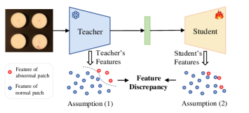
Figure 1: Illustration of Teacher-Student Feature Discrepancy, whose success relies on how to keep the feature discrepancy between teacher and student model. This line of methods have two assumptions: (1) the teacher encoder can jointly represent two different distributions for both normal and abnormal patterns; while (2) the student decoder can only reconstruct the normal distribution.

Recent advances [5, 6, 3, 7, 8] often adopt knowledge distillation to take advantage of the pre-trained model, which involves a multi-scale feature reconstruction of the pre-trained features. As shown in Fig. 1, it solves the anomaly detection problem by focusing on the “teacher-student discrepancy”, i.e., the feature discrepancy between a fixed pre-trained teacher encoder and a learnable student decoder. To make the “teacher-student discrepancy” hypothesis more robust, particularly ensuring larger discrepancies when anomalies are presented, two sub-assumptions need to be satisfied: (1) the teacher encoder can jointly represent two different distributions for the normal and abnormal patterns, while (2) the student decoder can only reconstruct the normal distribution. However, these ideal assumptions are hard to meet in practice, which requires researchers to improve them from different perspectives.

For the first assumption, it is important yet has been overlooked in current methods. As shown in Table I, we can observe a significant performance drop by randomly initializing the teacher model in the well-known RD [3] framework. Although the pre-trained model can alleviate this issue, it still remains a challenging issue to generate discriminative features in solving the IAD problem. To the best of our knowledge, the challenge mainly arises from two aspects: (1) Difference between task objectives. In pre-training on ImageNet, models aim to discriminate between different object categories; while in the IAD task, models need to discriminate between normal and abnormal instances within a single object category. (2) Scarcity of abnormal data. Abnormal objects are far less common than normal objects in the real world, therefore the models have fewer opportunities to learn representations of anomalies during pre-training. Due to these factors, the pre-trained embeddings may become over-compressed and learn some irrelevant semantics to the IAD task, which limits the pre-trained teacher model’s ability to discriminate between normal and abnormal industrial instances. When it comes to the second assumption, earlier methods [6, 3] give a natural constraint, i.e., anomalies cannot reconstruct abnormal representations since they are absent in the training process. To guarantee the student model consistently outputs normal patterns, some recent works [7, 8] impose stronger constraints on the student model to suppress anomaly signals. Despite these, less attention has been drawn to the reconstruction capacity of the student decoder in dealing with challenging normal patterns, such as the fine-grained normal textures and rare normal patterns.

TABLE I: Comparison of teacher model with different representation ability. “$\checkmark\kern-4.13332pt\raisebox{3.44444pt}{\rotatebox[origin={c}]{125.0}{{--}}}$” indicates the assumption is not fully guaranteed, and “I-AUC” represents the results on the VisA [9] dataset. For fair comparison, the training of the student model is set consistent.

Teacher model	Assump. (1)	Assump. (2)	I-AUC (%)
Random Teacher	$\times$	✓	81.3
Pre-trained Teacher (RD)	$\checkmark\kern-4.13332pt\raisebox{3.44444pt}{\rotatebox[origin={c}]{125.0}{{--}}}$	✓	96.2
Advanced Teacher (Ours)	✓	✓	97.8

To this end, we consider how to extend the teacher encoder’s discrimination capacity and how to enhance the student decoder’s normality distillation ability. In this paper, we propose a simple yet effective two-stage IAD framework to achieve robust feature discrepancy between the teacher and student model. Specifically, it consists of an anomaly amplification stage and a normality distillation stage, which address the first and second assumptions, respectively. In the first stage, we propose a novel Residual Anomaly Amplification (RAA) module to advance the fixed teacher with the exposure of synthetic anomalies. Considering over-reliance on synthetic anomalies may lead to catastrophic forgetting [10] of pre-trained knowledge, our RAA module employs a residual learning mechanism, which amplifies the sensitivity to anomalies while maintaining the integrity of pre-trained model. This module comprises two critical components: a matching-guided residual gate and an attribute-scaling residual generator, which determine the proportion and characteristics of residuals, respectively. In the second stage, we employ a reverse distillation paradigm to train a student decoder that can only reconstruct normal representations, in which a novel hard knowledge distillation (HKD) loss is built to better facilitate the reconstruction of normal patterns. Without losing generality, the teacher-student discrepancy is utilized for anomaly detection during inference. Comprehensive experiments on the MvTecAD, VisA, and MvTec3D-RGB datasets demonstrate the effectiveness of our method.

Our main contributions are as follows:

• We design a novel two-stage industrial anomaly detection framework based on the two assumptions of knowledge distillation, which can obtain robust feature discrepancy between the teacher and student model.

• We design a novel residual anomaly amplification module in the anomaly amplification stage, which can enhance the discrimination capacity of the vanilla teacher encoder with the help of synthetic anomalies.

• We design a novel hard knowledge distillation loss in the normality distillation stage, which can enhance the reconstruction capability of the student decoder in dealing with challenging normal patterns.

The rest of this paper is organized as follows. We review the related work in Section II. Section III describes the technical details of our proposed AAND. Section IV presents the experiment details and results. Finally, we summarize the paper in Section V.

II Related Work

In this section, we review some related works on IAD. The current works can be categorized into four types: reconstruction-based, synthesis-based, embedding-based, and distillation-based methods.

Reconstruction-based methods. As anomaly detection is typically treated as an unsupervised problem, reconstruction-based methods have emerged as a natural approach. It aims to reconstruct normal inputs and assumes that the reconstruction error is larger for anomalies. Early methods often employ GAN [11], AE [12, 13, 14, 15, 16], or VAE [17, 18] to train reconstruction models. To make the anomaly pixels more difficult to reconstruct, RIAD [19] proposes a reconstruction-by-inpainting approach, which removes partial pixels to reconstruct the images. Inspired by the ability of latent diffusion model [20, 21] in generating high-quality and diverse images, more and more recent approaches [22, 23, 24, 25] utilize diffusion models to model the image reconstruction as a denoising process. Nevertheless, the pixel-level reconstruction methods may easily generalize to anomalies, resulting in the well-reconstruction of some anomalies. To address this issue, some research has focused on exploring knowledge distillation, with a shift towards reconstructing inputs at the feature level.

Synthesis-based methods. Due to the lack of abnormal samples in training, it is challenging for the IAD task to find the boundary between normality and anomaly. Thus, synthesis-based methods propose to synthesize anomalies by introducing noises into normal images [26, 27, 28, 29]. For example, in the case of DRAEM [26], textures are sampled from an external texture dataset [30], and Perlin [31] noise is employed to generate random anomaly masks for creating anomalies. Besides, Cutpaste [27] randomly selects augmented regions from an image and pastes it onto other random regions of the image. NSA [28] employs Poisson image editing to seamlessly blend patches of varying sizes from different images. Additionally, some methods synthesize noise at the feature level, such as SimpleNet [32] and DSR [33]. However, real-world anomalies exhibit a wide range of patterns and uncertainties that cannot be fully covered. Consequently, over-reliance on synthetic anomalies may overfit the seen anomalies, while getting bad performance on unseen anomalies. In our method, we utilize synthetic anomalies to amplify the sensitivity of the pre-trained model to anomalies, while keeping its original discrimination ability on some unseen anomalies. To the best of our knowledge, we are the first to enhance the pre-trained teacher model with synthetic anomalies in solving the IAD problem.

Embedding-based methods. Thanks to the development of models pre-trained on extensive external datasets, such models can effectively represent both normal and abnormal patterns for anomaly detection. In practice, the embedding-based methods usually utilize ImageNet pre-trained models to encode normal samples into high-dimensional feature spaces. For example, Padim [34] calculates the inverse covariance matrix to model the normal distribution, Patchcore [2] stores representative features in memory banks, and M3DM [35] constructs multiple memory banks to store features from different modalities. What’s different, some methods [36, 4, 37, 38] employ additional decoders to learn the distribution of normal samples using normalizing flows [39]. For example, CS-Flow [37] proposes a simple framework that jointly processes multiple feature maps of different scales. Besides, CFlow [4] models a conditional normalizing flow with a position encoding, and adopts a multi-scale generative decoder to estimate the likelihood of encoded features. Since these methods largely rely on the pre-trained model, their performances are limited by the discrimination capacity of pre-trained model.

Distillation-based methods. This line of methods can combine the advantages of both reconstruction-based and embedding-based methods, which involve a student model to reconstruct the multi-scale pre-trained embeddings of a teacher model on normal samples. The mainstream methods can be roughly categorized into forward distillation and reverse distillation methods. In particular, the forward distillation approaches [5, 6] often adopt similar networks between student and teacher models to train the distillation process. Nevertheless, they suffer from the similarity of student and teacher architecture, where the abnormal data is mapped closely, resulting in an undesirably small feature discrepancy for anomalies. To address this issue, RD [3] adopts a reverse distillation paradigm. Rather than directly receiving raw images, the student network takes the one-class embedding of the teacher model as input, to restore the teacher’s multi-scale representations. Besides, AST [40] proposes a framework comprising a pre-trained encoder and two decoders, in which a normalizing flow decoder serves as a teacher for density estimation, while a conventional feed-forward network acts as a student. To guarantee the student network consistently outputs normal patterns, recent methods impose stronger constraints on the student network. For example, RD++ [7] introduces multi-scale projection layers and incorporates several loss constraints, so as to facilitate the student model in suppressing abnormal signals from pseudo-abnormal regions. Besides, DeSTSeg [8] introduces a denoising stage to train a denoising student that reconstructs the normal patterns both for normal and abnormal inputs.

However, most distillation-based methods solely focus on the student model, while overlooking the limited discrimination ability of the teacher model. Unlike previous methods, we both focus on enhancing the teacher model’s discrimination capacity and the student model’s normality distillation ability.

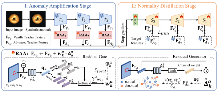
Figure 2: Overview of our proposed AAND.  I. Anomaly Amplification Stage: the vanilla teacher model encodes the input image into K-level features $\mathbf{F}_{T_{k}}$, and then these features are advanced to $\mathbf{F}_{A_{k}}$ through our proposed Residual Anomaly Amplification module (RAA). The RAA module effectively amplifies anomalies while preserving the integrity of the pre-trained model. It comprises a matching-guided residual gate and an attribute-scaling residual generator, which determine the proportion and characteristics of the residuals, respectively. II. Normality Distillation Stage: a student model decodes features $\mathbf{F}_{S_{k}}$, and these features are trained to distill the representation of advanced teacher only on normal samples, where “BN” denotes a bottleneck module and $\mathcal{L}_{HKD}$ represents our proposed Hard Knowledge Distillation loss. During inference, the “teacher-student discrepancy” is used for anomaly detection.

III Method

III-A Overview.

In the context of unsupervised industrial anomaly detection, Let $\mathcal{X}^{train}=\{\mathbf{I}_{1}^{n},\mathbf{I}_{2}^{n}...,\mathbf{I}_{N}^{n}\}$ be a training set containing only normal images, and $\mathcal{X}^{test}=\{\mathbf{I}_{1}^{t},\mathbf{I}_{2}^{t}...,\mathbf{I}_{M}^{t}\}$ be a test set including both normal and abnormal images. The goal of anomaly detection is to train a model to identify and localize anomalies in the test images.

As shown in Fig. 2, we propose a simple yet effective two-stage anomaly detection framework named AAND. It comprises an Anomaly Amplification Stage to enhance the teacher model’s discrimination capacity, and a Normality Distillation Stage to train the student model’s normality reconstruction ability. In the first stage, we synthesize anomalies to aid training and introduce a novel RAA module to advance the teacher model. Specifically, the RAA module not only amplifies anomalies but also preserves the integrity of the pre-trained model. It includes a matching-guided residual gate and an attribute-scaling residual generator, which regulate the proportion and characteristics of the residuals, respectively. In the subsequent stage, a reverse distillation paradigm is employed to train a student decoder, in which a novel HKD loss is proposed to reconstruct complex normal patterns effectively. During inference, anomaly detection is facilitated by exploiting the discrepancies between the teacher and student models.

III-B Anomaly Amplification Stage

ImageNet pre-trained encoders are widely used [2, 3, 7] in the industrial anomaly detection task, where the pre-trained embedding is directly used without any adaption. However, the gap between ImageNet pretraining and IAD task poses significant challenges in fulfilling the first assumption previously mentioned. To mitigate this issue, we introduce an anomaly amplification stage aimed at increasing the teacher model’s ability to discriminate between normal and anomalous patterns. The training within this stage incorporates synthetic anomalies and a novel RAA module.

Anomaly synthesis. Given the normal images from the training set $\mathcal{X}^{train}$, we use a widely used anomaly generator [26] to generate abnormal masks and images. First, Perlin noise [31] is generated and binarized into an anomaly mask $\mathbf{\overline{M}^{a}}$ $\in\{0,1\}^{H\times W}$ to determine the locations of anomalies. Then, texture samples are obtained from the source texture dataset [30] to serve as the content for these locations. For a normal image $\mathbf{I^{n}}$ $\in\mathbb{R}^{C\times H\times W}$, the corresponding synthetic abnormal image is denoted as $\mathbf{I^{a}}$ $\in\mathbb{R}^{C\times H\times W}$. Considering the anomalies are typically on the foreground object, we follow [41] to extract a foreground mask $\mathbf{\overline{M}^{f}}$ $\in\{0,1\}^{H\times W}$ with grayscale binary thresholding algorithms. The resulting pseudo-anomaly mask $\mathbf{\overline{M}}$ is then obtained by taking the intersection of the two masks.

During the first-stage training, we take the corrupted image $\mathbf{I^{a}}$ as input of the teacher encoder. The encoder extracts $K$-level features $\mathbf{F}_{T_{k}}\in\mathbb{R}^{C_{k}\times H_{k}\times W_{k}}$. At the k-th level of feature extraction, a total of $H_{k}\times W_{k}$ patches are obtained. By subsampling the anomaly mask at the same scale, denoted as $\mathbf{\overline{M}}_{k}$, and using it to label the normal and abnormal locations, these patches can be divided into $N_{k}^{n}$ normal patches and $N_{k}^{a}$ abnormal patches. The corresponding features are denoted as $\mathbf{F}_{T_{k}}^{n}\in\mathbb{R}^{N^{n}_{k}\times C_{k}}$ and $\mathbf{F}_{T_{k}}^{a}\in\mathbb{R}^{N^{a}_{k}\times C_{k}}$ respectively.

Residual Anomaly Amplification. With the introduction of synthetic anomalies, we then design a novel RAA module that utilizes a residual learning mechanism to enhance anomaly detection without compromising the integrity of the pre-trained model. This module comprises two critical components: a matching-guided residual gate and an attribute-scaling residual generator. As shown in Fig. 3, the residual gate suppresses residuals on normal samples to maintain the integrity of pre-trained model while encouraging residuals on synthetic inputs to promote deviations. Additionally, the residual generator is designed to adaptively learn the characteristics of residuals, which directly influence the distribution of emergent abnormal features. By embedding these RAA modules into the pre-existing framework, we have successfully crafted an advanced teacher encoder that robustly enhances anomaly detection capabilities. The extracted feature at the k-th block of the advanced teacher model, denoted as $\mathbf{F}_{A_{k}}\in\mathbb{R}^{C_{k}\times H_{k}\times W_{k}}$, is calculated as follows:

$$\mathbf{F}_{A_{k}}=\mathbf{F}_{T_{k}}+\mathbf{w}^{a}_{k}\cdot\mathbf{\Delta}_{k}^{a},$$ (1)

where $\mathbf{w}_{k}^{a}\in[0,1]^{H_{k}\times W_{k}}$ represents the anomaly weights predicted by the residual gate, and $\mathbf{\Delta}_{k}^{a}\in\mathbb{R}^{C_{k}\times H_{k}\times W_{k}}$ is the residual signals generated by the residual generator.

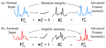
Figure 3: Illustration of our proposed RAA module. It utilizes a residual learning mechanism to amplify anomalies while maintaining the integrity of pre-trained model.

III-B1 Matching-guided residual gate

This module aims to regulate the proportion of residuals, which functions as a robust binary classifier that predicts the weight of anomalies. This prediction is informed by the matching results between the queries and the stored memory items.

As illustrated in Fig. 2, we take the feature map $\mathbf{F}_{T_{k}}\in\mathbb{R}^{C_{k}\times H_{k}\times W_{k}}$ extracted from the frozen teacher block as input. The input is first added with a position encoding $\mathbf{p}_{c}$ [37], and then passed through an MLP, $\Phi_{\theta_{1}}^{k}(\cdot)$, for projection:

$$\mathbf{q}_{k}^{i}=\Phi_{\theta_{1}}^{k}(\mathbf{F}_{T_{k}}^{i}+\mathbf{p}_{c}^{i}),$$ (2)

where $\mathbf{F}_{T_{k}}^{i}\in\mathbb{R}^{C}$ and $\mathbf{p}_{c}^{i}\in\mathbb{R}^{C}$ are the input feature and position encoding at the $i$-th patch, respectively. In addition, $\mathbf{q}_{k}^{i}\in\mathbb{R}^{C}$ represents the projected feature. To represent the memory of normality and anomaly, we configure a normal memory $\mathbf{M}_{k}^{n}=\{\mathbf{m}_{k1}^{n},\mathbf{m}_{k2}^{n},...,\mathbf{m}_{kL}^{n}\}$ containing $L$ learnable normal embeddings, and an anomaly memory $\mathbf{M}^{a}_{k}=\{\mathbf{m}_{k1}^{a},\mathbf{m}_{k2}^{a},...,\mathbf{m}_{kL}^{a}\}$ containing $L$ learnable anomaly embeddings. Subsequently, a matching process is conducted between the query and memories, which involves computing their cosine similarity and normalizing the similarity scores using the softmax function. Consequently, the normal weights, denoted as $w^{n}_{kj},j\in\{1,2,...,L\}$, and the anomaly weights, denoted as $w^{a}_{kj},j\in\{1,2,...,L\}$, are derived as follows:

$$w^{n}_{kij}=\frac{\mathrm{exp}(s(\mathbf{q}_{k}^{i},\mathbf{m}^{n}_{kj}))}{Z}, \,w^{a}_{kij}=\frac{\mathrm{exp}(s(\mathbf{q}_{k}^{i},\mathbf{m}^{a}_{kj}))}{Z},$$ (3)

where $Z$ represents the normalization factor, ensuring that $\sum_{j=1}^{L}w^{n}_{kij}+\sum_{j=1}^{L}w^{a}_{kij}=1$. When presented with an abnormal patch query $\mathbf{q}_{k}^{a}$, it has a higher affinity to the anomaly memory. Conversely, for a normal patch query $\mathbf{q}_{k}^{n}$, it has a higher affinity to the normal memory. By matching different abnormal features and normal features, the dual memories will learn the different feature distributions. Afterwards, the sum of anomaly weights is taken as the outputs of the residual gate:

$$w_{ki}^{a}=\sum_{j=1}^{L}w^{a}_{kij}=1-\sum_{j=1}^{L}w^{n}_{kij},$$ (4)

where the anomaly weight $w^{a}_{ki}\in[0,1]$ represents the anomaly probability of inputs. Within the entire RAA module, its role is to control the proportion of residual generation. To supervise the anomaly weight, we adopt the well-known focal loss [42]. The ground truth $\overline{w}^{a}_{ki}\in\{0,1\}$ is from the pseudo-anomaly mask $\mathbf{\overline{M}}_{k}$, which equals to 1 when it is a synthetic abnormal patch, while equaling to 0 when it is a normal patch.

III-B2 Attribute-scaling residual generator

Due to the influence of residual characteristics on the distribution of new abnormal features, we address this challenge by introducing an attribute-scaling residual generator. The residual noise aims to emphasize the attributes that are relevant to anomalies while diminishing those irrelevant attributes. Specifically, the key designs are the channel weight module and the anomaly amplification loss.

As illustrated in Fig. 2, we initiate the process by projecting $\mathbf{F}_{T_{k}}^{i}$ using another MLP, denoted as $\Phi_{\theta_{2}}^{k}(\cdot)$. Subsequently, each channel of the projected feature is mapped to the range (-1,1) through a tanh function, yielding scaling weights $\mathbf{\Sigma}^{i}_{k}\in\mathbb{R}^{C}$ for each channel. Finally, the generated residual $\mathbf{\Delta}_{k}^{a_{i}}\in\mathbb{R}^{C}$ is calculated by multiplying the channel weights and input features as follows:

$$\mathbf{\Delta}_{k}^{a_{i}}=\mathrm{Tanh}(\Phi_{\theta_{2}}^{k}(\mathbf{F}_{T_{k}}^{i}))\odot\mathbf{F}_{T_{k}}^{i},$$ (5)

where $\odot$ denotes element-wise multiplication. To obtain the updated features and avoid interfering with the parameters of the residual gate, we replace the predicted anomaly weights $\hat{w}_{i}^{a}$ with the ground truth anomaly weights $\overline{w}_{i}^{a}$ during training as follows:

$$\mathbf{F}_{A_{k}}^{n_{i}}=\mathbf{F}_{T_{k}}^{n_{i}}+0\cdot\mathbf{\Delta}^{a_{i}}_{k},\quad\mathbf{F}_{A_{k}}^{a_{i}}=\mathbf{F}_{T_{k}}^{a_{i}}+1\cdot\mathbf{\Delta}^{a_{i}}_{k},$$ (6)

where the superscripts $a_{i}$ and $n_{i}$ denote the abnormal and normal patches, respectively. Here, $\mathbf{F}_{A_{k}}^{a_{i}}$ represents the learnable features updated by the residuals, while $\mathbf{F}_{T_{k}}^{a_{i}}$, $\mathbf{F}_{A_{k}}^{n_{i}}$, and $\mathbf{F}_{T_{k}}^{n_{i}}$ remain frozen. This ensures that the optimization is confined exclusively to the synthetic anomaly features, specifically on the residual $\mathbf{\Delta}^{a_{i}}_{k}$.

To supervise the residuals, we propose an anomaly amplification loss to push the abnormal features outside the boundaries of normality, which is calculated as follows:

$$\mathcal{L}_{\mathrm{A}}=\frac{1}{N^{a}_{k}N^{n}_{k}}\sum\limits_{i=1}^{N^{a}_{k}}\sum\limits_{j=1}^{N^{n}_{k}}\mathrm{max}(s(\mathbf{F}^{a_{i}}_{A_{k}},\mathbf{F}^{n_{j}}_{T_{k}}),\mathbf{S}^{ref}_{kij}),$$ (7)

where $\mathbf{S}^{ref}_{k}\in\mathbb{R}^{N^{a}_{k}\times N^{n}_{k}}$ is a dynamic margin matrix calculated based on the similarity matrix produced by the vanilla teacher model, which is denoted as follows:

$$\mathbf{S}_{kij}^{ref}=s(\mathbf{F}^{a_{i}}_{T_{k}},\mathbf{F}^{n_{j}}_{T_{k}})-\alpha,$$ (8)

where $\alpha$ is a hyper-parameter to control the degree of reduction. It is noteworthy that the loss function $\mathcal{L}_{A}$ is specifically designed to reduce the similarity between abnormal and normal features. For normal samples, we utilize the residual gate to suppress the residuals instead of pulling them as in standard contrastive learning. This approach preserves the integrity of the pre-trained model, thereby preserving its ability to capture a diverse representation of normal samples.

The overall loss of this stage is summarized as follows:

$$\mathcal{L}_{1}=\mathcal{L}_{focal}+\mathcal{L}_{A},$$ (9)

where the focal loss and anomaly amplification loss supervise the anomaly weight $\mathbf{w}^{a}_{k}$ and the residual signals $\mathbf{\Delta}^{a}_{k}$, respectively.

III-C Normality Distillation Stage

Upon enhancing the discrimination capabilities of the teacher encoder, our objective shifts to training a student decoder, specially designed to reconstruct only the normal distribution. To accomplish this, we employ a reverse distillation paradigm [3] to train the student decoder. Within this framework, we introduce a hard knowledge distillation loss, specifically designed to improve the reconstruction of normal patterns.

In this stage, the advanced teacher is fixed and only receives normal samples. Its output normal features $\mathbf{F}^{n}_{A_{k}}\in\mathbb{R}^{C_{k}\times H_{k}\times W_{k}}$ are then passed to a one-class bottleneck embedding module [3], which aggregates the multi-scale embeddings to obtain a compact representation. Subsequently, the learnable student decoder predicts multi-scale features $\mathbf{F}^{n}_{S_{k}}\in\mathbb{R}^{C_{k}\times H_{k}\times W_{k}}$, which is trained to fit the target features from the teacher model using a knowledge distillation loss:

$$\mathcal{L}_{KD}=\ 1-s(\mathbf{\tilde{F}}^{n}_{A_{k}},\mathbf{\tilde{F}}^{n}_{S_{k}}),$$ (10)

where the features $\mathbf{\tilde{F}}^{n}_{A_{k}}\in\mathbb{R}^{C_{k}H_{k}W_{k}}$ and $\mathbf{\tilde{F}}^{n}_{S_{k}}\in\mathbb{R}^{C_{k}H_{k}W_{k}}$ are obtained by flattening the features $\mathbf{F}^{n}_{A_{k}}$ and $\mathbf{F}^{n}_{S_{k}}$ through vectorization, respectively. By exclusively training with normal samples and leveraging the compact embedding design of reverse distillation [3], the student decoder will be effectively constrained to reconstruct only the normal distribution.

Furthermore, considering the difficulty in accurately reconstructing the features of certain fine-grained normal textures and rare normal patterns, we propose a hard knowledge distillation loss as follows:

$$\mathcal{L}_{HKD}=\,\frac{1}{K_{h}}\sum_{d=1}^{K_{h}}(1-s(\mathbf{F}^{n_{d}}_{A_{k}}.\mathbf{F}^{n_{d}}_{S_{k}})),$$ (11)

where $K_{h}$ represents the number of selected hard samples, while $\mathbf{F}^{n_{d}}_{A_{k}}$ and $\mathbf{F}^{n_{d}}_{A_{k}}$ denote the selected features. As illustrated in Fig. 4, the HKD loss specifically emphasizes the distillation of the top-$K_{h}$ hard normal instances, which helps the student decoder to achieve a more accurate reconstruction of these challenging patterns.

The overall loss function for the normality distillation stage is formulated as follows:

$$\mathcal{L}_{2}=\mathcal{L}_{KD}+\mathcal{L}_{HKD}.$$ (12)

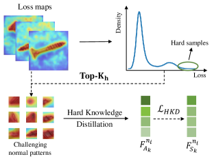
Figure 4: Illustration of our proposed HKD loss. It facilitates the reconstruction on challenging normal patterns by selecting the $K_{h}$ normal patches with the highest distillation loss for further training.

To summarize the two-stage training procedure of our AAND, we show the pseudo-code in Algorithm 1.

1 $T$: Teacher, $R$: RAA module, $A$: Advanced Teacher $B$: Bottleneck, $S$: Student decoder, subscript $k$: block index, superscript $a$: anomaly, $n$: normal

/* Stage1: Anomaly Amplification */

2 for  $\mathbf{I}^{a}\leftarrow$ Synthesis Dataloader do

3       $\mathbf{F}_{T_{1}},\mathbf{F}_{T_{2}},\mathbf{F}_{T_{3}}$ $\leftarrow T(\mathbf{I}^{a})$;

4       $w_{k}^{a},\Delta_{k}^{a}\leftarrow R_{k}(\mathbf{F}_{T_{k}})$; // RAA module

5       $\mathbf{F}_{A_{k}}\leftarrow\mathbf{F}_{T_{k}}+w_{k}^{a}\cdot\Delta_{k}^{a}$;

6       $\mathcal{L}_{1}\leftarrow\mathcal{L}_{focal}+\mathcal{L}_{A}$;

7       Optimize $R$ by $\mathcal{L}_{1}$;

8 end for

/* Stage2: Normality Distillation */

9 for  $\mathbf{I}^{n}\leftarrow$ Train Dataloader do

10       $\mathbf{F}^{n}_{A_{1}},\mathbf{F}^{n}_{A_{2}},\mathbf{F}^{n}_{A_{3}}\leftarrow$ Stage1;

11       $\mathbf{F}_{S_{1}}^{n},\mathbf{F}_{S_{2}}^{n},\mathbf{F}_{S_{3}}^{n}$ $\leftarrow S(B(\mathbf{F}_{A_{1}}^{n},\mathbf{F}_{A_{2}}^{n},\mathbf{F}_{A_{3}}^{n}))$;

12       $\mathcal{L}_{2}\leftarrow\mathcal{L}_{KD}+\mathcal{L}_{HKD}$;

13       Optimize $B$ and $S$ by $\mathcal{L}_{2}$;

14 end for

Algorithm 1 Pseudo-code of AAND training

III-D Inference

During inference, the anomaly detection is based on the feature discrepancy between the advanced teacher model and the student model. Given a test image $\mathbf{I}^{t}$, the advanced teacher encoder extracts $K$-level features $\mathbf{F}_{A_{k}}$, then the student decoder aggregates the features and reconstructs the multi-scale features $\mathbf{F}_{S_{k}}$. The feature discrepancy, denoted as $D(\mathbf{F}_{A_{k}},\mathbf{F}_{S_{k}})$, is calculated using the negative cosine similarity as follows:

$$D(\mathbf{F}_{A_{k}},\mathbf{F}_{S_{k}})=1-s(\mathbf{F}_{A_{k}},\mathbf{F}_{S_{k}}).$$ (13)

The advanced teacher model is capable of generating discriminative features for both normal and abnormal inputs, whereas the student network is tailored to reconstruct only the normal features. This configuration results in a minor feature discrepancy in normal samples, while a pronounced discrepancy when anomalies are present. To effectively localize anomalies, anomaly maps are generated across the $K$ network blocks. These maps are then upsampled and aggregated to obtain an anomaly score for each pixel:

$$\mathbf{\hat{S}}_{A}=\sum_{l=1}^{K}\mathrm{Up}_{k}(D(\mathbf{F}_{A_{k}},\mathbf{F}_{S_{k}})),$$ (14)

where $\mathbf{\hat{S}}_{A}$ is the predicted anomaly score map, and $\mathrm{Up}_{k}(\cdot)$ denotes the bi-linear up-sampling. A higher score in the anomaly map indicates a higher likelihood of anomaly at that position, and the maximum value in the anomaly map is considered as the image-level anomaly score.

IV Experiments

IV-A Dataset

To assess the effectiveness of the proposed method, we conduct comprehensive experiments on three datasets: MVTec AD [43], Visa [9] and MVTec3D-RGB [44].

MVTec AD. It is a well-studied benchmark for anomaly detection and localization. It consists of 3,629 anomaly-free training images, and 1,725 testing images, which include both normal and abnormal samples. The dataset has been widely explored with the results almost reaching saturation.

VisA. It is a large industrial anomaly detection dataset that is composed of 10,821 high-resolution color images of 12 objects. The anomaly type covers both surface and structural defects. The dataset is more challenging than MvTec AD. It not only contains multiple instances of a single object category but also has different types of Printed Circuit Boards (PCB) with complex structures.

MVTec3D-RGB. It is a multi-modal dataset that comprises 2,656 training 2D-3D pairs and 1,197 testing 2D-3D pairs. Some anomalies are more significant in geometry while having subtle changes in appearance, making it particularly challenging to detect anomalies based solely on the visual appearance of RGB images. Considering the computational cost associated with using point cloud data, we follow the recent work [41] to employ only the RGB images for anomaly detection and localization.

TABLE II: Anomaly detection and localization performance on the MVTec AD [43], VisA [9] and MvTec3D-RGB [44] dataset. Since the MVTec AD benchmark has approached saturation, our method shows only slight enhancements. When applied to the more challenging VisA and MVTec3D-RGB datasets, more significant improvements can be observed.

	Method	Venue	MvTec AD			VisA			MvTec3D-RGB
			I-AUC	P-AUC	PRO	I-AUC	P-AUC	PRO	I-AUC	P-AUC	PRO
Others	DRAEM [26]	ICCV’21	98.0	97.3	-	88.7	93.5	72.4	75.7	97.6	-
	PaDiM [34]	ICPR’21	95.5	97.3	92.1	89.1	98.1	85.9	76.4	-	-
	Patchcore [2]	CVPR’22	99.1	98.1	94.4	95.1	98.8	91.2	77.0	96.6	87.6
	CFLow [4]	WACV’22	98.3	98.0	94.6	93.2	98.4	89.0	85.1	97.4	-
	SimpleNet [32]	CVPR’23	99.6	98.1	-	80.8	89.5	69.4	84.1	96.0	88.0
	FOD [41]	ICCV’23	99.2	98.3	-	93.7	98.4	-	88.4	97.6	-
KD	ST [5]	BMVC’21	95.5	97.0	92.1	83.3	-	62.0	-	-	-
	RD [3] (baseline)	CVPR’22	98.5	98.3	94.0	96.2	98.6	93.4	88.5	99.0	96.7
	RD++ [7]	CVPR’23	99.4	98.3	95.0	96.0	98.6	93.2	88.2	99.0	97.2
	DeSTSeg [8]	CVPR’23	98.6	97.9	-	91.2	98.0	90.2	86.3	96.7	89.8
	Ours		99.5	98.4	95.0	98.1	99.0	94.8	90.6	99.2	97.5

TABLE III: I-AUC for anomaly detection performance of all object categories on the challenging VisA [9] dataset.

Method	Venue	candle	capsules	cashew	chewing	fryum	maca-	maca-	pcb1	pcb2	pcb3	pcb4	pipe	mean
					gum		roni1	roni2					fryum
Patchcore [2]	CVPR’22	98.6	81.6	97.3	99.1	96.2	97.5	78.1	98.5	97.3	97.9	99.6	99.8	95.1
SPD [9]	ECCV’22	89.1	68.1	90.5	99.3	89.8	85.7	70.8	92.7	87.9	85.4	99.1	95.6	87.8
RD[3]	CVPR’22	95.3	90.7	97.0	99.1	96.5	96.5	90.6	97.0	96.9	95.5	99.5	99.5	96.2
RD++ [7]	CVPR’23	96.0	91.4	97.0	99.1	95.5	97.0	88.9	97.1	96.2	94.9	99.5	99.6	96.0
Ours		98.4	92.3	98.0	99.7	98.0	99.6	95.2	98.4	98.9	98.7	99.9	99.9	98.1

TABLE IV: I-AUC for anomaly detection performance of all object categories on the challenging MVTec3D-RGB [44] datasets.

Method	Venue	bagel	cable	carrot	cookie	dowel	foam	peach	potato	rope	tire	mean
			gland
Patchcore[2]	CVPR’22	87.6	88.0	79.1	68.2	91.2	70.1	69.5	61.8	84.1	70.2	77.0
M3DM [35]	CVPR’23	94.4	91.8	89.6	74.9	95.9	76.7	91.9	64.8	93.8	76.7	85.0
RD[3]	CVPR’22	98.5	96.2	96.5	64.5	99.1	83.6	91.4	68.0	99.4	87.7	88.5
RD++ [7]	CVPR’23	99.4	91.5	94.4	69.7	98.6	82.6	92.7	69.5	97.7	85.5	88.2
Ours		99.3	96.3	96.9	71.2	99.3	86.8	93.0	71.2	99.5	92.7	90.6

IV-B Implementation Details

Experimental settings. We utilize the WideResNet50 [45] encoder as the backbone with the output embeddings from three layers ($K=3$). During training, images are resized into 256 × 256, batch size is set to 16, and Adam is used as the optimizer with a learning rate of 0.005. We train the first stage for 100 epochs and then train the second stage for another 120 epochs. Besides, the hyper-parameters $\alpha$, $L$, and $K_{h}$ are set to 0.3, 50, and 10, respectively. For the synthetic anomalies, we follow [38] to extract foreground masks with grayscale binary thresholding algorithms to control the noise only in the foreground, which brings the synthesis closer to real conditions.

Evaluation metrics. We evaluate the AD performance using the area under the receiver operator curve (AUROC) based on the generated anomaly scores. We utilize image-level AUROC (I-AUC) to evaluate anomaly detection performance, while pixel-based AUROC (P-AUC) and the PRO metric [46] were employed to assess anomaly localization.

IV-C Main Results

We conduct a comprehensive comparison of the performance of anomaly detection and localization. We mainly compare the Knowledge Distillation-based (KD) methods [5, 3, 8, 7] and other popular paradigms for anomaly detection, such as reconstruction-based approaches [43, 41], synthesis-based methods [26, 32], and embedding-based methods [2, 4]. For the MvTec AD dataset [43], reported results are directly obtained from the published papers. For the newly published VisA [9] and MVTec3D-RGB [44] datasets, due to some anomaly detection methods have not yet been evaluated on these datasets, we re-train them using their open-source code and evaluate their performance on both datasets.

Table II shows the comparison results of anomaly detection and localization on the MVTec AD, VisA, and MVTec3D-RGB benchmarks. In the widely studied MVTec AD dataset, our method slightly outperforms the current state-of-the-art methods. Since the anomalies of this dataset are relatively easier to identify, the current methods have already achieved a high level of performance, leaving limited potential for substantial advancements. In the VisA and MVTec3D datasets, our method surpasses the current state-of-the-art approaches significantly. Compared to the well-known method PatchCore [2], our method takes advantage of the enhanced feature encoder and robust knowledge distillation paradigm, leading to better performances. Compared to the synthesis-based method SimpleNet [32], our approach achieves comparable results on the MvTec dataset, while demonstrating significant improvements on the more challenging Visa and Mvtec3D-RGB datasets. This observation indicates the robustness of our method in handling more complex industrial datasets. Compared with our baseline RD, our proposed method improves the image-level AUROC and pixel-level PRO by 1.0%, 1.0% on MvTec AD, 1.9%, 1.4% on VisA, 2.1%, 0.8% on Mvtec3D-RGB.

Thanks to the enhanced discrimination capability of our advanced teacher model, our method demonstrates the ability to effectively detect previously undetectable anomalies. Table III and Table IV present the anomaly detection performance for each object in VisA and MVTec3D-RGB datasets, respectively. These two datasets contain difficult anomaly instances, such as capsules, macaroni2, potato, and tire, that exhibit subtle variations in appearance compared to normal instances, posing significant challenges to anomaly detection. Remarkably, our method achieves a 1.6% improvement in the “capsules” category, a 4.6% improvement in the “macarnoni2” category, a 1.7% improvement in the potato category, and a 5.0% improvement in the tire category. These results highlight the effectiveness of our approach in overcoming the limited discrimination capacity of pre-trained models and effectively identifying challenging anomalies.

TABLE V: Ablation Study of main modules of our framework. MRG and ARG are the sub-modules of RAA proposed in the first stage. $\mathcal{L}_{HKD}$ is the hard knowledge distillation loss proposed in the second stage.

Exp.	MRG	ARG	$\mathcal{L}_{HKD}$	MvTec AD			VisA			MvTec3D-RGB
				I-AUC	P-AUC	PRO	I-AUC	P-AUC	PRO	I-AUC	P-AUC	PRO
base				98.5	98.3	94.0	96.2	98.6	93.4	88.5	99.0	96.7
(a)	✓			94.4	94.7	89.6	90.7	95.3	88.2	81.2	97.6	91.7
(b)		✓		98.7	96.9	90.3	97.1	98.6	92.5	87.1	98.1	93.2
(c)	✓	✓		99.3	98.1	94.7	97.8	98.8	94.7	90.1	99.1	97.2
(d)			✓	99.1	97.9	94.3	97.4	98.6	93.7	89.6	98.9	96.6
(e)	✓	✓	✓	99.5	98.4	95.0	98.1	99.0	94.8	90.6	99.2	97.5

IV-D Ablation Study

Ablation of main components. In this part, we conduct an ablation study on the main components of our model: RAA module proposed in the first stage and HKD loss proposed in the second stage. In detail, RAA comprises a Matching-based Residual Gate (MRG) and Attribute-scaling Residual Generator (ARG). We utilize the RD [3] as the baseline and compare the following settings: (a) directly utilizing the predicted anomaly weight from MRG as the anomaly score, (b) blindly generating residuals using ARG without considering the anomaly weight from MRG, (c) incorporating both MRG and ARG, i.e., the RAA module, (d) solely introducing the HKD loss to the baseline, and (e) employing all the components. As shown in Table V (a)-(c), the integration of MRG and ARG is essential for the advance of the vanilla teacher model to achieve better performance. On one hand, solely relying on MRG may be limited to synthetic anomalies, which will be further discussed in the subsequent ablation study. On the other hand, generating an equal proportion of residuals for both normal and abnormal samples disrupts the discrimination ability of the pre-trained model, resulting in an ambiguous representation space. The results of (c) and (e) show the effectiveness of the hard knowledge distillation loss, which enhances the student’s ability to accurately reconstruct the features of certain fine-grained normal textures and rare normal patterns. By using all the components, our method can not only extend the pre-trained teacher’s representation ability but also enhance the student’s normal distillation ability, which satisfies the first and second assumptions in the distillation-based methods.

TABLE VI: Comparison of different discrimination methods for advancing the pre-trained teacher models.

Method	MvTec AD		VisA		MvTec3D-RGB
	I-AUC	PRO	I-AUC	PRO	I-AUC	PRO
(a) Contrastive	73.7	43.3	61.2	23.4	59.9	34.2
(b) SimpleNet	99.6	-	80.8	69.4	84.1	88.0
(c) Our MRG	94.4	94.7	90.7	88.2	81.2	91.7
(d) Our AAND	99.5	95.0	98.1	94.8	90.6	97.5

Comparison of alternative discrimination methods. Our primary objective is to augment the discrimination capacity of the pre-trained teacher model by leveraging synthetic anomalies. We compare our proposed method with three alternative discrimination-based approaches: (a) Contrastive learning: In the first stage, the teacher model is trained to pull the distances of normal features closer, while pushing the distances between normal features and anomalous features further apart. Besides, the second distillation stage is identical to ours. (b) Using the synthetic noise and binary classification method proposed by SimpleNet [32]. (c) Directly using the anomaly score predicted by our MRG module for anomaly detection. As shown in Table VI (a)-(c), these simpler discrimination methods yield suboptimal results. The reason is that they overfit synthesized anomalies, resulting in a learned decision boundary with limited generalizability to real anomalies. To the best of our knowledge, SimpleNet achieves the best performance on the MvTec Dataset, possibly because it is easier to synthesize anomalies similar to real anomalies in this dataset. However, when confronted with more challenging datasets, its performance tends to be comparatively lower. This could be attributed to the disruption of the pre-trained prior and the absence of robust knowledge distillation techniques. In our two-stage framework, our anomaly amplification stage enhances the discrimination capacity of the pre-trained mode while preserving its integrity. Additionally, we employ a normality distillation stage to further clarify the normality boundary using the available normal data.

TABLE VII: Analysis of the residual properties in the ARG module.

Method	MvTec AD		VisA		MvTec3D-RGB
	I-AUC	PRO	I-AUC	PRO	I-AUC	PRO
(a) Learnable residuals	98.2	94.8	94.5	94.2	85.6	96.0
(b) ARG w/ sigmoid	99.5	94.4	97.6	94.2	90.0	97.0
(c) ARG w/ tanh	99.5	95.0	98.1	94.8	90.6	97.5

TABLE VIII: Comparison of distillation-based approaches in terms of inference time, network parameters, and performance (I-AUC/P-AUC/PRO) on the MVTec 3D-RGB dataset.

Method	Infer. time (s)	Parameters (MB)	Performance (%)
RD	0.024	161.08	88.5 / 99.0 / 96.7
RD++	0.027	176.57	88.2 / 99.0 / 97.2
Ours	0.027	170.45	90.6 / 99.2 / 97.5

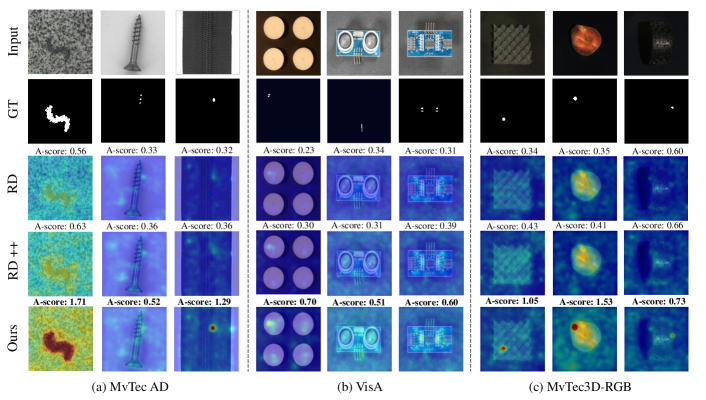
Figure 5: Qualitative results for anomaly localization, where “A-score” denotes the maximum value in the anomaly score map. Compared to RD [3] and RD++ [7], our method can accurately localize anomalies even in some challenging cases where the abnormal region is extremely small or the appearance of the anomaly is very similar to normal data.

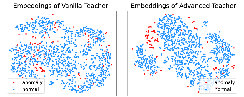
(a) candle class

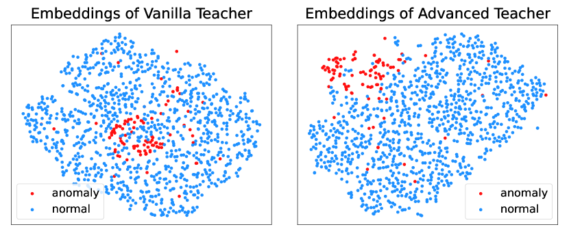
(b) macaroni2 class

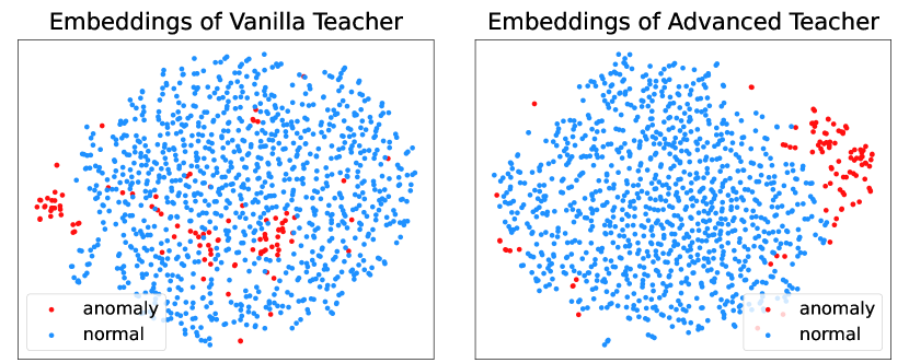
(c) bagel class

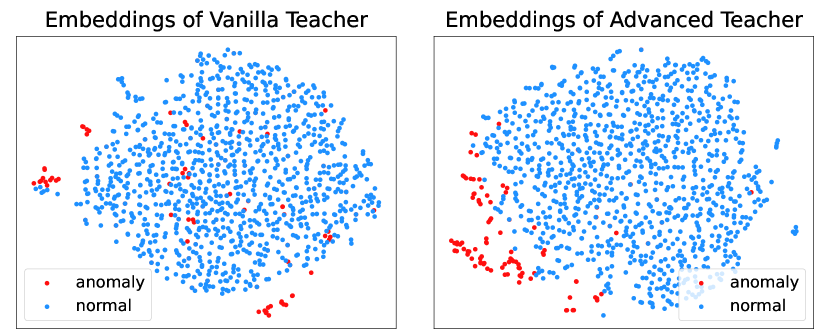
(d) foam class

Figure 6: Comparison of feature distribution between the vanilla teacher model and our advanced teacher model, visualized using t-SNE [47]. (a)-(d) represent specific industrial product categories from the benchmark datasets. Our method demonstrates a significantly enhanced discrimination capacity between normal and abnormal inputs.

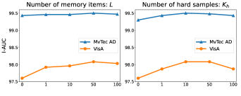
Figure 7: Hyper-parameter sensitivity analysis for the number of memory items $L$ and the number of hard samples $K_{h}$, evaluated on the MvTec AD [43] and VisA  [9] datasets.

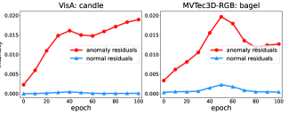
Figure 8: The variation of the intensity of residuals with respect to training epochs. The blue line indicates the residual variation on normal samples, while the red line indicates the residual variation on anomaly samples.

Analysis of residual properties. To understand the impact of different residual characteristics in the ARG module, we conduct ablation studies that are shown in Table VII. It involves (a) replacing the residuals in Eq. (5) with learnable residuals, and (b) replacing the tanh function in Eq. (5) with a sigmoid function. The utilization of learnable residuals without explicit scale restrictions can potentially result in excessive residuals and the disruption of the pre-trained model’s prior knowledge. In contrast to scaling the residuals to the range (0, 1) using the sigmoid function, we employ the tanh function to project the residuals to the range of (-1, 1). This choice leads to moderate perturbations to the original features, thus improving the performance effectively.

Model complexity analysis. We compare the inference speed and number of parameters between our approach and existing distillation-based methods on MVTec3D-RGB dataset. The experiment is conducted on a Nvidia GeForce GTX 2080ti GPU with Intel(R) Xeon(R) CPU E5-2680 v4@ 2.40GHZ. Inference time includes both model inference time and anomaly map computation time in average, and batch size is set to 1 during testing. As shown in Table VIII, our method introduces a marginal increase in inference time compared to RD and possesses fewer parameters than RD++. In comparison to the one-stage baseline RD, our two-stage framework solely incorporates the lightweight RAA modules, resulting in a slight computational overhead but a remarkable enhancement in performance.

Hyper-parameter sensitivity. There are two important hyper-parameters in our method: the number of memory items $L$ in MRG module, and the number of the selected hard sample $K_{h}$ in the hard knowledge distillation loss. We evaluate the sensitivity of our model to the two parameters on the MvTec AD [43] and VisA [9] datasets. We first fix $K_{h}$ at 10 to change $L$, and then fix $L$ to the best value to change $K_{h}$. As shown in Fig. 7, MRG demonstrates robustness concerning the memory size $L$. Appropriately increasing the memory size helps to capture the diversity of normality and anomaly, where we observe that the best performance is achieved when the memory size is set to 50. For the number of hard samples $K_{h}$, compared to not selecting hard samples (i.e., $K_{h}=0$), selecting different numbers of hard samples can improve performance. The best performance is achieved when $K_{h}=10$. Insufficient hard samples lack representativeness of challenging patterns, while an excessive amount of hard samples hinders the model’s focus on the most challenging patterns.

IV-E Visualization Analysis

Qualitative results for anomaly localization. We present qualitative anomaly localization results in Fig. 5. Compared to RD and RD++, our method can accurately localize anomalies even in some challenging cases, where the abnormal region is extremely small or the appearance of the anomaly is very similar to normal data. When dealing with these cases, the vanilla teacher model in RD and RD++ maps abnormal inputs to a normal representation, in which the student also constructs the normality. As a result, some defective products cannot be successfully detected due to the unreliable teacher-student feature discrepancy. Unlike these methods, our advanced teacher model can generate more discriminative features, which better fulfills the first assumption in distillation-based anomaly detection methods. In practice, detecting these challenging anomalies helps manufacturers identify problems promptly and ensures that consumers receive satisfactory products.

Visualization of feature distribution. To demonstrate the enhanced discrimination capacity of our anomaly amplification stage, we present the visualization of feature distribution in Fig. 6. Without the introduced stage, the feature distribution of the vanilla teacher exhibits ambiguity between normal and abnormal features. Our method enhances the prominence of anomalies while maintaining the integrity of the pre-trained embedding. As illustrated in Fig. 6, the diversity of normal embeddings is preserved, and the anomalies are effectively pushed away from the boundary of normality.

Visualization of residual variation. Our proposed RAA module suppresses the residuals on normal features while encouraging residuals for abnormal features. To demonstrate this, we present visualizations of residual variations during training in Fig. 8. We define the intensity of residual noises for normal samples and anomaly samples as $\frac{1}{N^{n}\times C}\sum_{i=1}^{N^{n}}\sum_{j=1}^{C}{(\Delta^{n}_{ij})^{2}}$ and $\frac{1}{N^{a}\times C}\sum_{i=1}^{N^{a}}\sum_{j=1}^{C}{(\Delta^{a}_{ij})^{2}}$, respectively. During the training process, the intensity of residual noise is kept minimal for normal samples, thereby preserving the pre-trained model’s fidelity to normal instances. Conversely, the residuals on abnormal inputs exhibit an increasing trend, amplifying the distinctions between anomalies and normal instances.

V Conclusion

In this paper, we propose a novel two-stage industrial anomaly detection framework, which sequentially performs anomaly amplification and normality distillation to obtain robust feature discrepancy. In the first anomaly amplification stage, we propose a novel residual anomaly amplification module to advance the teacher model with the exposure of synthetic anomalies. It effectively amplifies anomalies via residual generation while maintaining the integrity of the pre-trained model. In the second normality distillation stage, we design a novel hard knowledge distillation loss, which enhances the reconstruction capability of the student decoder in dealing with challenging normal patterns. Comprehensive experiments on the MvTecAD, VisA, and MvTec3D-RGB dataset demonstrate the effectiveness of our method.

Limitation and future work: Some hard anomalies are still difficult to detect solely from RGB images. Combining knowledge from other modalities, such as point clouds and natural language, may lead to better detection results. In addition, synthesizing anomaly data that closely resembles real-world anomalies is crucial for better advancing pre-trained models. These will be explored in our future work.

References

- [1] J. Deng, W. Dong, R. Socher, L.-J. Li, K. Li, and L. Fei-Fei, “Imagenet: A large-scale hierarchical image database,” in 2009 IEEE conference on computer vision and pattern recognition. Ieee, 2009, pp. 248–255.
- [2] K. Roth, L. Pemula, J. Zepeda, B. Schölkopf, T. Brox, and P. Gehler, “Towards total recall in industrial anomaly detection,” in Proceedings of the IEEE/CVF Conference on Computer Vision and Pattern Recognition, 2022, pp. 14 318–14 328.
- [3] H. Deng and X. Li, “Anomaly detection via reverse distillation from one-class embedding,” in Proceedings of the IEEE/CVF Conference on Computer Vision and Pattern Recognition, 2022, pp. 9737–9746.
- [4] D. Gudovskiy, S. Ishizaka, and K. Kozuka, “Cflow-ad: Real-time unsupervised anomaly detection with localization via conditional normalizing flows,” in Proceedings of the IEEE/CVF Winter Conference on Applications of Computer Vision, 2022, pp. 98–107.
- [5] G. Wang, S. Han, E. Ding, and D. Huang, “Student-teacher feature pyramid matching for anomaly detection,” arXiv preprint arXiv:2103.04257, 2021.
- [6] M. Salehi, N. Sadjadi, S. Baselizadeh, M. H. Rohban, and H. R. Rabiee, “Multiresolution knowledge distillation for anomaly detection,” in Proceedings of the IEEE/CVF conference on computer vision and pattern recognition, 2021, pp. 14 902–14 912.
- [7] T. D. Tien, A. T. Nguyen, N. H. Tran, T. D. Huy, S. Duong, C. D. T. Nguyen, and S. Q. Truong, “Revisiting reverse distillation for anomaly detection,” in Proceedings of the IEEE/CVF Conference on Computer Vision and Pattern Recognition, 2023, pp. 24 511–24 520.
- [8] X. Zhang, S. Li, X. Li, P. Huang, J. Shan, and T. Chen, “Destseg: Segmentation guided denoising student-teacher for anomaly detection,” in Proceedings of the IEEE/CVF Conference on Computer Vision and Pattern Recognition, 2023, pp. 3914–3923.
- [9] Y. Zou, J. Jeong, L. Pemula, D. Zhang, and O. Dabeer, “Spot-the-difference self-supervised pre-training for anomaly detection and segmentation,” in European Conference on Computer Vision. Springer, 2022, pp. 392–408.
- [10] J. Kirkpatrick, R. Pascanu, N. Rabinowitz, J. Veness, G. Desjardins, A. A. Rusu, K. Milan, J. Quan, T. Ramalho, A. Grabska-Barwinska et al., “Overcoming catastrophic forgetting in neural networks,” Proceedings of the national academy of sciences, vol. 114, no. 13, pp. 3521–3526, 2017.
- [11] A. Creswell, T. White, V. Dumoulin, K. Arulkumaran, B. Sengupta, and A. A. Bharath, “Generative adversarial networks: An overview,” IEEE signal processing magazine, vol. 35, no. 1, pp. 53–65, 2018.
- [12] M. Rudolph, B. Wandt, and B. Rosenhahn, “Structuring autoencoders,” in Proceedings of the IEEE/CVF International Conference on Computer Vision Workshops, 2019, pp. 0–0.
- [13] D. Gong, L. Liu, V. Le, B. Saha, M. R. Mansour, S. Venkatesh, and A. v. d. Hengel, “Memorizing normality to detect anomaly: Memory-augmented deep autoencoder for unsupervised anomaly detection,” in Proceedings of the IEEE/CVF International Conference on Computer Vision, 2019, pp. 1705–1714.
- [14] L. Wang, J. Tian, S. Zhou, H. Shi, and G. Hua, “Memory-augmented appearance-motion network for video anomaly detection,” Pattern Recognition, vol. 138, p. 109335, 2023.
- [15] J. Hou, Y. Zhang, Q. Zhong, D. Xie, S. Pu, and H. Zhou, “Divide-and-assemble: Learning block-wise memory for unsupervised anomaly detection,” in Proceedings of the IEEE/CVF International Conference on Computer Vision, 2021, pp. 8791–8800.
- [16] S. Lu, W. Zhang, H. Zhao, H. Liu, N. Wang, and H. Li, “Anomaly detection for medical images using heterogeneous auto-encoder,” IEEE Transactions on Image Processing, 2024.
- [17] D. P. Kingma and M. Welling, “Auto-encoding variational bayes,” arXiv preprint arXiv:1312.6114, 2013.
- [18] J. Li, Q. Huang, Y. Du, X. Zhen, S. Chen, and L. Shao, “Variational abnormal behavior detection with motion consistency,” IEEE Transactions on Image Processing, vol. 31, pp. 275–286, 2021.
- [19] V. Zavrtanik, M. Kristan, and D. Skočaj, “Reconstruction by inpainting for visual anomaly detection,” Pattern Recognition, vol. 112, p. 107706, 2021.
- [20] R. Rombach, A. Blattmann, D. Lorenz, P. Esser, and B. Ommer, “High-resolution image synthesis with latent diffusion models,” in Proceedings of the IEEE/CVF conference on computer vision and pattern recognition, 2022, pp. 10 684–10 695.
- [21] J. Ho, A. Jain, and P. Abbeel, “Denoising diffusion probabilistic models,” Advances in neural information processing systems, vol. 33, pp. 6840–6851, 2020.
- [22] J. Wyatt, A. Leach, S. M. Schmon, and C. G. Willcocks, “Anoddpm: Anomaly detection with denoising diffusion probabilistic models using simplex noise,” in Proceedings of the IEEE/CVF Conference on Computer Vision and Pattern Recognition, 2022, pp. 650–656.
- [23] Y. Teng, H. Li, F. Cai, M. Shao, and S. Xia, “Unsupervised visual defect detection with score-based generative model,” arXiv preprint arXiv:2211.16092, 2022.
- [24] F. Lu, X. Yao, C.-W. Fu, and J. Jia, “Removing anomalies as noises for industrial defect localization,” in Proceedings of the IEEE/CVF International Conference on Computer Vision, 2023, pp. 16 166–16 175.
- [25] X. Zhang, N. Li, J. Li, T. Dai, Y. Jiang, and S.-T. Xia, “Unsupervised surface anomaly detection with diffusion probabilistic model,” in Proceedings of the IEEE/CVF International Conference on Computer Vision, 2023, pp. 6782–6791.
- [26] V. Zavrtanik, M. Kristan, and D. Skočaj, “Draem-a discriminatively trained reconstruction embedding for surface anomaly detection,” in Proceedings of the IEEE/CVF International Conference on Computer Vision, 2021, pp. 8330–8339.
- [27] C.-L. Li, K. Sohn, J. Yoon, and T. Pfister, “Cutpaste: Self-supervised learning for anomaly detection and localization,” in Proceedings of the IEEE/CVF conference on computer vision and pattern recognition, 2021, pp. 9664–9674.
- [28] H. M. Schlüter, J. Tan, B. Hou, and B. Kainz, “Natural synthetic anomalies for self-supervised anomaly detection and localization,” in European Conference on Computer Vision. Springer, 2022, pp. 474–489.
- [29] M. Z. Zaheer, J.-H. Lee, A. Mahmood, M. Astrid, and S.-I. Lee, “Stabilizing adversarially learned one-class novelty detection using pseudo anomalies,” IEEE Transactions on Image Processing, vol. 31, pp. 5963–5975, 2022.
- [30] M. Cimpoi, S. Maji, I. Kokkinos, S. Mohamed, and A. Vedaldi, “Describing textures in the wild,” in Proceedings of the IEEE conference on computer vision and pattern recognition, 2014, pp. 3606–3613.
- [31] K. Perlin, “An image synthesizer,” ACM Siggraph Computer Graphics, vol. 19, no. 3, pp. 287–296, 1985.
- [32] Z. Liu, Y. Zhou, Y. Xu, and Z. Wang, “Simplenet: A simple network for image anomaly detection and localization,” in Proceedings of the IEEE/CVF Conference on Computer Vision and Pattern Recognition, 2023, pp. 20 402–20 411.
- [33] V. Zavrtanik, M. Kristan, and D. Skočaj, “Dsr–a dual subspace re-projection network for surface anomaly detection,” in European conference on computer vision. Springer, 2022, pp. 539–554.
- [34] T. Defard, A. Setkov, A. Loesch, and R. Audigier, “Padim: a patch distribution modeling framework for anomaly detection and localization,” in International Conference on Pattern Recognition. Springer, 2021, pp. 475–489.
- [35] Y. Wang, J. Peng, J. Zhang, R. Yi, Y. Wang, and C. Wang, “Multimodal industrial anomaly detection via hybrid fusion,” in Proceedings of the IEEE/CVF Conference on Computer Vision and Pattern Recognition, 2023, pp. 8032–8041.
- [36] M. Rudolph, B. Wandt, and B. Rosenhahn, “Same same but differnet: Semi-supervised defect detection with normalizing flows,” in Proceedings of the IEEE/CVF winter conference on applications of computer vision, 2021, pp. 1907–1916.
- [37] M. Rudolph, T. Wehrbein, B. Rosenhahn, and B. Wandt, “Fully convolutional cross-scale-flows for image-based defect detection,” in Proceedings of the IEEE/CVF Winter Conference on Applications of Computer Vision, 2022, pp. 1088–1097.
- [38] X. Yao, R. Li, J. Zhang, J. Sun, and C. Zhang, “Explicit boundary guided semi-push-pull contrastive learning for supervised anomaly detection,” in Proceedings of the IEEE/CVF Conference on Computer Vision and Pattern Recognition, 2023, pp. 24 490–24 499.
- [39] D. Rezende and S. Mohamed, “Variational inference with normalizing flows,” in International conference on machine learning. PMLR, 2015, pp. 1530–1538.
- [40] M. Rudolph, T. Wehrbein, B. Rosenhahn, and B. Wandt, “Asymmetric student-teacher networks for industrial anomaly detection,” in Proceedings of the IEEE/CVF Winter Conference on Applications of Computer Vision, 2023, pp. 2592–2602.
- [41] X. Yao, R. Li, Z. Qian, Y. Luo, and C. Zhang, “Focus the discrepancy: Intra-and inter-correlation learning for image anomaly detection,” in Proceedings of the IEEE/CVF International Conference on Computer Vision, 2023, pp. 6803–6813.
- [42] T.-Y. Lin, P. Goyal, R. Girshick, K. He, and P. Dollár, “Focal loss for dense object detection,” in Proceedings of the IEEE international conference on computer vision, 2017, pp. 2980–2988.
- [43] P. Bergmann, M. Fauser, D. Sattlegger, and C. Steger, “Mvtec ad–a comprehensive real-world dataset for unsupervised anomaly detection,” in Proceedings of the IEEE/CVF conference on computer vision and pattern recognition, 2019, pp. 9592–9600.
- [44] P. Bergmann, X. Jin, D. Sattlegger, and C. Steger, “The mvtec 3d-ad dataset for unsupervised 3d anomaly detection and localization,” arXiv preprint arXiv:2112.09045, 2021.
- [45] S. Zagoruyko and N. Komodakis, “Wide residual networks,” arXiv preprint arXiv:1605.07146, 2016.
- [46] P. Bergmann, M. Fauser, D. Sattlegger, and C. Steger, “Uninformed students: Student-teacher anomaly detection with discriminative latent embeddings,” in Proceedings of the IEEE/CVF conference on computer vision and pattern recognition, 2020, pp. 4183–4192.
- [47] L. Van der Maaten and G. Hinton, “Visualizing data using t-sne.” Journal of machine learning research, vol. 9, no. 11, 2008.