Few-sample Variational Inference of Bayesian Neural Networks with Arbitrary Nonlinearities

Abstract

Bayesian Neural Networks (BNNs) extend traditional neural networks to provide uncertainties associated with their outputs. On the forward pass through a BNN, predictions (and their uncertainties) are made either by Monte Carlo sampling network weights from the learned posterior or by analytically propagating statistical moments through the network. Though flexible, Monte Carlo sampling is computationally expensive and can be infeasible or impractical under resource constraints or for large networks. While moment propagation can ameliorate the computational costs of BNN inference, it can be difficult or impossible for networks with arbitrary nonlinearities, thereby restricting the possible set of network layers permitted with such a scheme. In this work, we demonstrate a simple yet effective approach for propagating statistical moments through arbitrary nonlinearities with only 3 deterministic samples, enabling few-sample variational inference of BNNs without restricting the set of network layers used. Furthermore, we leverage this approach to demonstrate a novel nonlinear activation function that we use to inject physics-informed prior information into output nodes of a BNN.

1 Introduction

Bayesian Neural Networks (BNNs) [1, 2] treat learnable parameters of a neural network as distributions, enabling predictive power and training insights generally not available from traditional neural networks. Of particular interest is their ability to express calibrated uncertainties in their predictions, a feature that makes BNNs desirable in many (if not most) real-world applications.

In the context of Bayesian inference, BNNs are trained to learn the posterior distribution of network weights given the observed data and prior distributions over the weights. Since computing the true posterior distribution is generally intractable, approximate inference techniques, such as variational inference, are often used [3, 4, 5]. With the variational approximation, BNN inference becomes practical and often relatively simple to implement, for instance using Bayes by backprop [6]. Despite the relative ease of implementation, BNN inference can be prohibitively expensive computationally in some applications, such as when compute resources are limited or when the number of learnable weight distributions is especially large.

Using the mean-field approximation (i.e., weights are conditionally independent given the data and hence the posterior is factorized as a product of the weight densities) and assuming Normally distributed weights, converting a standard neural network to a BNN at most doubles the number of learnable parameters (the mean and variance of each weight distribution) and hence is not particularly taxing computationally. During inference, however, the need for Monte Carlo sampling can require 10s or 100s of samples to accurately characterize the output distribution, particularly for regression tasks. Alternatively, the need for Monte Carlo sampling can be eliminated or greatly reduced by propagating statistical moments (e.g., mean and variance) through the network, providing a deterministic prediction with reduced computational complexity [7, 8, 9]. Unfortunately, existing moment propagation-based inference techniques only work on a restricted set of network layers, with addition of new layers requiring analytic derivation or approximation of associated propagation rules (see, for example, the equations needed to propagate a Normally distributed random variable through the popular leaky-ReLU activation presented in [9]) or yet again relying on Monte Carlo sampling. The lack of extensibility to novel nonlinearities reduces the potential impact of moment propagation-based BNN inference.

In this work, we present an effective and relatively straightforward method to enable moment propagation through BNNs with arbitrary nonlinearities. In particular, we show that the unscented transform [10] (popularized in Kalman filtering applications) enables few-sample deterministic BNN inference with significantly reduced computational costs compared to Monte Carlo sampling without sacrificing performance. We demonstrate the utility of the unscented transform for BNN inference on a simple multi-layer perceptron with known analytic propagation rules and on a more complex convolutional neural network with a novel, application-specific activation function for which analytic moment propagation rules have not been derived.

2 Background

2.1 Variational inference of Bayesian neural networks

Our terminal objective for BNN inference is to estimate a predictive distribution that describes the probability of observing an output (denoted by $\mathbf{y}$) given an input (denoted by $\mathbf{x}$) conditioned on the previous observations. For instance, we may wish to estimate the position of an object (output) within an image (input), in which case we seek a distribution over possible positions conditioned on the image. We denote our BNN by the distribution $p(\mathbf{y}|\mathbf{x},\mathbf{w})$ parameterized by weights $\mathbf{w}$. The training data is denoted as $\mathcal{D}\equiv\{(x_{i},y_{i})\}_{i=1}^{m}$. The desired predictive distribution is thus

$$p(\mathbf{y}|\mathbf{x},\mathcal{D}) =\mathbb{E}_{p(\mathbf{w}|\mathcal{D})}[p(\mathbf{y}|\mathbf{x},\mathcal{D},\mathbf{w})]$$

$$=\int d\mathbf{w}\,p(\mathbf{y}|\mathbf{x},\mathcal{D},\mathbf{w})p(\mathbf{w}|\mathcal{D})$$ (1)

The variational approximation involves replacing the (generally intractable) distribution $p(\mathbf{w}|\mathcal{D})$ by a variational distribution $q(\mathbf{w}|\mathbf{\theta})$ parameterized by learnable parameters $\theta$.

2.1.1 Monte Carlo sampling

Although the variational approximation simplifies BNN inference, computing the integral in Eqn. 2.1 remains intractable in general. As such, Monte Carlo sampling is often employed to approximate the integral [2, 6]. This is achieved by taking $n$ samples from the variational posterior $q(\mathbf{w}|\mathbf{\theta})$ (which, by design, we can sample from) and computing the associated $n$ forward passes $\{\mathbf{y}_{j}\}_{j=1}^{n}$ through the BNN. Moments of the predictive distribution are then computed as needed, for example the expected value and variance of $\mathbf{y}$

$$\mathbb{E}[\mathbf{y}] =\int d\mathbf{y}\,\mathbf{y}p(\mathbf{y}|\mathbf{x},\mathcal{D})\approx\frac{1}{n}\sum_{j=1}^{n}\mathbf{y}_{j}=\bar{\mathbf{y}}$$

$$\mathbb{V}[\mathbf{y}] \approx\frac{1}{n-1}\sum_{j=1}^{n}(\mathbf{y}_{j}-\bar{\mathbf{y}})^{2}$$

2.1.2 Moment propagation

Monte Carlo integration of Eqn. 2.1 is computationally expensive and in some use cases may not be practical. As an example, consider using a BNN to solve a 1-dimensional regression task where the data are Normally distributed as $y|x\sim\mathcal{N}(\mu(x),\sigma(x)^{2})$. The standard error of the posterior predictive mean $\hat{\bar{y}}$ computed from $n$ independent Monte Carlo samples of the BNN would be $\mathrm{se}(\hat{\bar{y}})=\sigma/\sqrt{n}$, hence estimating the posterior predictive mean with standard error of $0.1\sigma$ would require at least 100 samples. Such a large number of samples is not practical when compute resources are limited or for large networks.

The above example motivates a more computationally efficient inference approach. Thankfully, under the mean-field approximation that neurons are conditionally independent, it is possible to analytically propagate the mean and variance through many common network layers (e.g., fully-connected, convolution, average pool) by taking advantage of simple properties of mean and variance of independent random variables:

$$\mathbb{E}[aX+b] =a\mathbb{E}[X]+b$$

$$\mathbb{V}[aX+b] =a^{2}\mathbb{V}[X]$$

$$\mathbb{E}[XY] =\mathbb{E}[X]\mathbb{E}[Y]$$

$$\mathbb{V}[XY] =\mathbb{V}[X]\mathbb{V}[Y]+\mathbb{V}[X]\mathbb{E}[Y]^{2}+\mathbb{E}[X]^{2}\mathbb{V}[Y]$$ (2)

These properties were used in [7, 8, 9] to eliminate the need for Monte Carlo sampling. For nonlinear layers, we must appeal to additional assumptions and more complicated computations, e.g., for ReLU [8] or leaky-ReLU [9]. In practice, this restricts the set of layers available to us within these inference frameworks to those for which analytic expressions of their moments are available, or otherwise requires us to again use Monte Carlo sampling for those layers.

3 Few-sample variational inference

In this section, we describe a simple technique for propagating mean and variance through nonlinear network layers. Our approach leverages the unscented transform popular in Kalman filtering, which allows us to approximate the effect of nonlinear network layers on an input distribution using only a few deterministic samples. Below, we describe the basics of the unscented transform and describe our implementation.

3.1 Unscented transform

To motivate the unscented transform, consider Normally distributed observations $x\sim\mathcal{N}(\mu,\sigma^{2})$. A nonlinear function $f$ transforms the observations as $f(x)$ and we wish to compute $\mathbb{E}[f(x)]$ and $\mathbb{V}[f(x)]$. One approach would be to linearize $f$, which would allow us to use the properties in Eqn. 2.1.2 to propagate mean and variance through $f$. Alternatively, we could transform random samples $x$ with the true nonlinear function $f$ and compute descriptive statistics from the result, as done in Monte Carlo sampling. Linearization requires us to compute the Jacobian and thus precludes application to “black box” nonlinearities [10] while Monte Carlo sampling is computationally expensive, hence neither approach is particularly appealing. This is the motivation for the unscented transform.

Briefly, the unscented transform involves selecting a small number (typically at least $2d+1$ in $d$ dimensions) of deterministic “sigma points” in the domain of the nonlinearity, transforming the sigma points, and then computing descriptive statistics of the transformed sigma points. Given sigma points $\{\chi_{k}\}_{k=1}^{s}$ and associated weights $\{\gamma_{k}\}_{k=1}^{s}$, the mean and variance of the distribution of $f(x)$ are approximated from the $s$ transformed sigma points as

$$\mathbb{E}[f(x)] \approx\sum_{k=1}^{s}\gamma_{k}f(\chi_{k})=\bar{f}$$ (3)

$$\mathbb{V}[f(x)] \approx\sum_{k=1}^{s}\gamma_{k}(f(\chi_{k})-\bar{f})^{2}$$ (4)

Sigma points and their associated weights are defined from the input distribution such that $\sum_{k=1}^{s}\gamma_{k}\chi_{k}=\mu$ and $\sum_{j=1}^{m}\gamma_{k}(\chi_{k}-\mu)^{2}=\sigma^{2}$.

3.2 Our approach

To achieve few-sample variational inference of BNNs, we use the unscented transform to propagate the mean and variance through layers of our BNN. We use this approach in conjunction with the analytical moment propagation method in [9], for instance to propagate through layers where propagation rules are unknown or intractable.

In this work, we use the mean-field approximation and assume the learnable parameters $\mathbf{w}$ of our BNNs are Normally distributed, hence our variational posterior takes the form $q(\mathbf{w}|\theta)=\prod_{j=1}^{m}q(w_{j}|\mu_{j},\sigma_{j}^{2})$ where $q$ is the density of the Normal distribution with parameters $\theta=\{(\mu_{j},\sigma_{j}^{2})\}_{j=1}^{M}$. We additionally assume that outputs of each layer parameterized by $w_{j}$ is again Normally distributed. We note that the unscented transform can be applied even when $q(\mathbf{w}|\theta)$ is not isotropic, however we do not explore that case here. Furthermore, the recently developed generalized unscented transform [11] could be used to eliminate the need to assume Normality.

To propagate through the nonlinear layers of our network, we note that the mean-field approximation allows us to apply a one dimensional unscented transform independently for each operation parameterized by $w_{j}$. For each input $x_{i}\sim\mathcal{N}(\mu_{i},\sigma_{i}^{2})$, we define sigma points and associated weights as in [10]:

$$\chi_{0,i} =\mu_{i},\quad \gamma_{0,i} =\frac{\kappa}{\kappa+1}$$

$$\chi_{1,i} =\mu_{i}-\sigma_{i}\sqrt{\kappa+1},\quad \gamma_{1,i} =\frac{1}{2(\kappa+1)}$$

$$\chi_{2,i} =\mu_{i}+\sigma_{i}\sqrt{\kappa+1},\quad \gamma_{2,i} =\frac{1}{2(\kappa+1)}$$ (5)

where $\kappa$ is a parameter used to influence the spread of sigma points. In this work, we use $\kappa=2$, though in principle allowing a learnable $\kappa>0$ may be beneficial. The mean and variance of $f(x_{i})$ is then computed using Eqns. 3 and 4 using the sigma points and weights in Eqn. 3.2. This process is repeated for all layer inputs $i$ and is then continued sequentially through the forward pass of the network, eventually yielding a mean and variance estimate for each output node of the BNN.

4 Experimental demonstration

In this section, we demonstrate our few-sample BNN inference approach on regression tasks solved by Bayesian fully-connected networks and Bayesian convolutional neural networks. For each experiment, we compare our results to those obtained by Monte Carlo sampling moment propagation through network nonlinearities. Unless otherwise noted, propagation through remaining network layers (e.g., linear layers) is performed using the method presented in [9]. We use the following notation to indicate which method is used to propagate moments through network nonlinearites: “MCVI” (Monte Carlo variational inference) for Monte Carlo sampling, “SMP” (simplified moment propagation) for purely analytical propagation as in [9], and “UTVI” (unscented transform variational inference) for the unscented transform method described in Section 3.2.

4.1 Training details

All networks were trained using the AdamW optimizer [12] with a learning rate $\alpha=0.01$, $\beta_{1}=0.9$, $\beta_{2}=0.999$, $\epsilon=10^{-8}$, and a weight decay $\lambda=0.01$. We used Bayes by backprop [6] with the Normal distribution likelihood for the likelihood term in the ELBO loss. We scaled the KL-loss term of the ELBO at each epoch $l=1,2,\ldots,M$ by a multiplicative factor $\phi(l)=\frac{2^{M-l}}{2^{M}-1}$ as in [9]. All results shown were averaged over 10 networks trained identically from randomly seeded initializations. We trained all networks using purely synthetic data generated on-the-fly, so networks never saw the same data more than once during training.

4.2 Regression with a fully-connected BNN

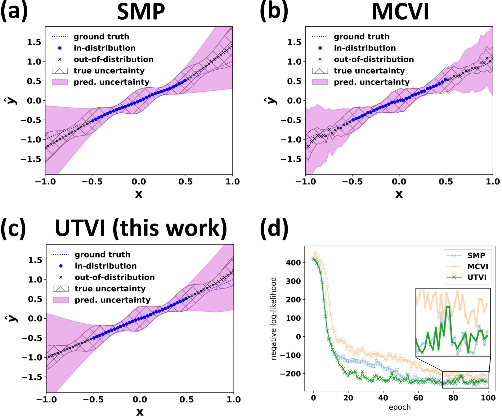
Figure 4: UTVI outperforms MCVI and matches SMP. Example results from a single model (for each of SMP, MCVI, and UTVI) for comparison to the averages over 10 models shown in Figure 1. Note that MCVI predictions are noisier than apparent from the model averaged results.

As an initial proof-of-concept, we use a fully-connected BNN with two hidden layers to model the function $y=x+\epsilon(x)$ where $\epsilon(x)\sim\mathcal{N}(0,\sigma(x)^{2})$ and $\sigma(x)=0.1+0.2\sin{(2\pi x-\pi/2)}^{2}$. Each hidden layer consists of 128 neurons and a leaky-ReLU activation. This problem serves as a convenient baseline because, for Normally distributed data, we can analytically propagate through the network using the SMP method (i.e., we can analytically compute $p(\mathbf{y}|\mathbf{x},\mathbf{w})$). For MCVI, we propagate moments through the leaky-ReLU layers with $n=3$ Monte Carlo samples (for a direct comparison to the 3 samples used for UTVI). For UTVI, we propagate moments through the leaky-ReLU layers with 3 sigma points as described in Section 3.2. The results of this experiment are shown in Figure 1, wherein all results were averaged over 10 independently trained model seeds (see Figure 4 for an example of single-model results). Qualitatively, UTVI (Figure 1(c)) matches the performance of SMP (Figure 1(a)) while exceeding the performance of MCVI (Figure 1(b)). Interestingly, as seen in Figure 1(d), UTVI seems to have better training characteristics as compared to SMP. We posit that this is due to the reduced number of floating point operations used by UTVI as compared to analytical moment propagation through the leaky-ReLU layers in the network (see [9] for analytical propagation rules), hence UTVI may have more numerically stable gradients during training.

To emphasize the savings in computational costs achieved by UTVI, we tracked the compute time needed for forward passes through each network on data batches of size 1024, with the number of samples used for MCVI varying until reaching comparable performance (in terms of the minimum validation set negative log-likelihood achieved during training) to UTVI. The results of this study are shown in Figure 2. As seen in Figure 2(a), UTVI with 3 sigma points exceeds the performance of MCVI until roughly $2^{7}$ Monte Carlo samples are used. Accordingly, as shown in Figure 2, UTVI is approximately 10X more computationally efficient than MCVI at a comparable level of performance. Furthermore, we see that UTVI matches the performance of SMP (Figure 2(a)) with comparable computational costs (Figure 2(b)).

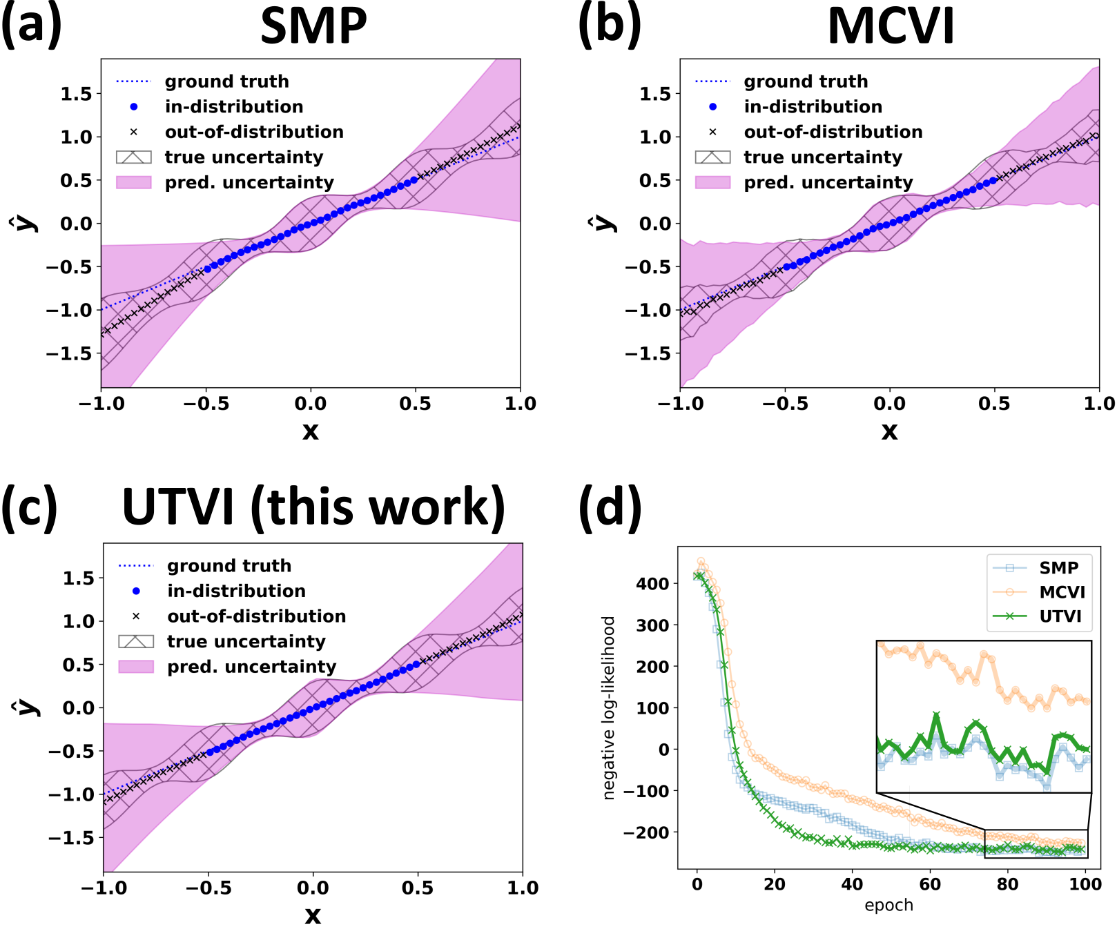
Figure 1: UTVI outperforms MCVI and matches SMP. BNN predictions using (a) SMP, (b) MCVI with 3 samples, and (c) UTVI. All data points represent the average over 10 networks trained independently from distinct random seeds. Note that MCVI with 3 samples appears less noisy than expected due to the averaging over 10 networks (see Figure 4 for an example output from a single network). “true uncertainty” is defined as $\sqrt{\epsilon(x)^{2}+\delta(x)^{2}}$ where $\epsilon(x)$ is the standard deviation of the simulated noise and $\delta(x)$ is the observed deviation from the prediction to the ground truth. (d) Reconstruction loss after each epoch (negative log-likelihood of in-distribution validation given the trained model) averaged across each of the 10 networks.

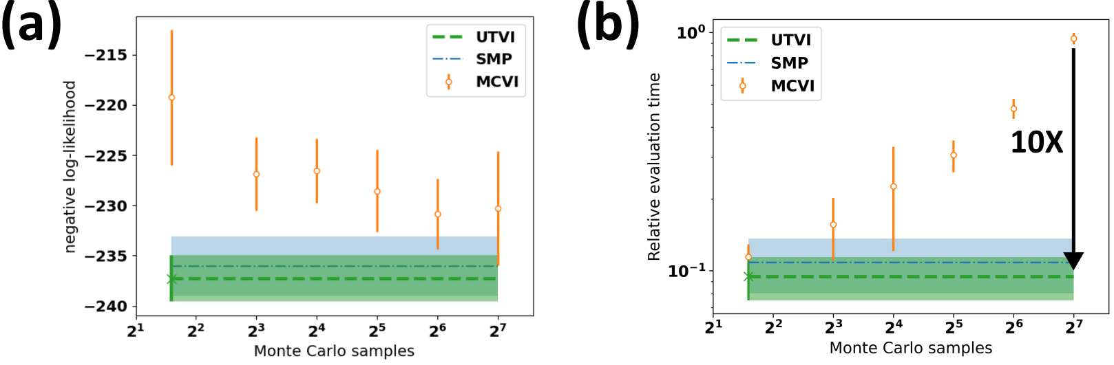
Figure 2: UTVI is 10X faster than MCVI at similar level of performance. (a) Minimum negative log-likelihood achieved by the best models on the evaluation set for MCVI models trained and evaluated with a varying number of samples. All data points shown were averaged over 10 independently trained models initialized with different random seeds. Error bars indicate $\pm$1 standard deviation over the 10 models. “Best” models were selected by taking the training checkpoint that achieved the lowest negative log-likelihood over the evaluation set. Results from UTVI with 3 samples and SMP (sampling-free) are shown for comparison. (b) Relative evaluation time averaged over 10 batches of 1024 network evaluations on an NVIDIA RTX A1000 laptop GPU. At $2^{7}$ samples (with which MCVI achieves roughly the same performance as UTVI), inference using UTVI is approximately 10X faster than with MCVI.

4.3 Sub-pixel object localization

To demonstrate UTVI on a more practically-relevant task, we use a convolutional BNN to quantify physical characteristics of an object within an image. Specifically, we use a BNN to estimate the two-dimensional position of a simulated fluorescent molecule imaged by a pixelated sensor, as well as the total number of photons incident on the sensor (a common task in, e.g., localization microscopy [13, 14, 15], where predictive uncertainties are necessary for subsequent analyses). For this task, we are particularly interested in injecting physics-informed constraints or other prior knowledge to restrict or otherwise guide the BNN towards a certain solution space. For example, we may have prior knowledge that the object of interest is likely to be well-centered within the image, or that the total number of collected photons follows a known distribution. We describe this experiment in more detail in the following sections.

4.3.1 Simulation

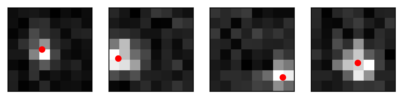
Figure 5: Examples of simulated object localization data. Random examples of data generated by the simulator described in Section 4.3.1. Red dots are added for visualization to indicate the ground truth object position and are not included during network training or evaluation. Images were rescaled independently to improve visualization.

To simulate data pairs $(\mathbf{x}_{i},\mathbf{y}_{i})=(\mathbf{x}_{i},[\mathbf{r}_{i},N_{i}(\mathbf{r}_{i})])$, we sample a two-dimensional emitter position $\mathbf{r}_{i}\sim\mathcal{N}(\mathbf{0},\sigma_{\mathrm{r}}^{2}\mathbf{I})$ with $\sigma_{\mathrm{r}}=2$ pixels, place a Gaussian blob with standard deviation $\sigma_{b}=0.21\lambda/\mathrm{na}=1.05$ pixels (the Gaussian point spread function standard deviation [16] corresponding to a simulated emission wavelength of 6 pixels measured with numerical aperture $\mathrm{na}=1.2$) normalized to integrate to $N=100$ photons at $\mathbf{r}_{i}$ in a pixelated image, and then corrupt the image with Poisson noise to yield $\mathbf{x}_{i}$. Note that our final image is a square with side length of $L=8$ pixels, so the detected photon count $N_{i}\leq N$ decreases for emitters near the edge of the image. Examples of simulated data are provided in Figure 5.

4.3.2 Injecting prior knowledge into BNN output nodes

To incorporate prior knowledge about our data into the BNN, we implement custom nonlinear activation functions at the output nodes of our BNN. We aim to mimic inverse transform sampling by using a (to the best of our knowledge) novel activation chain consisting of a scale function $f(x)$ that transforms inputs as $f:x\rightarrow[0,1]$ followed by the inverse cumulative distribution $F^{-1}(f(x))$ of a prior distribution on the output node. Ideally, the scale function should satisfy $f(x)\sim\mathcal{U}(0,1)$; in practice, we have observed the sigmoid function $f(x)=1/(1+\exp(-x/a))$ with learnable parameter $a$ to achieve our intended outcome.

For the output nodes predicting $\mathbf{r}_{i}$, we choose the prior $\mathcal{N}(\mathbf{0},\sigma^{2}\mathbf{I})$ with $\sigma=2$, biasing predicted positions towards the center of the image.

For the output node predicting the measured photon count, we choose the prior $\mathcal{N}(\mu=N_{i}(\hat{\mathbf{r}}_{i}),\sigma^{2}=N_{i}(\hat{\mathbf{r}}_{i}))$ to approximate the Poisson distribution with mean $N_{i}(\hat{\mathbf{r}}_{i})$. This activation, which is applied after computing position nodes, allows us to inject known physics into our network: the number of collected photons is (1) expected to be Poisson and (2) dependent on the position of the emitter within the restricted field of view captured by the image. During inference, we estimate $N_{i}$ by integrating an isotropic Normal distribution with mean $\hat{\mathbf{r}}_{i}$ and variance $\sigma_{b}^{2}$ over the image domain:

$$N_{i}(\hat{\mathbf{r}}_{i}) =\frac{N}{2\pi\sigma_{b}^{2}}\int_{L\times L}d\mathbf{r}\,\exp{\left(-\frac{(\mathbf{r}-\hat{\mathbf{r}}_{i})^{2}}{2\sigma_{b}^{2}}\right)}$$

$$=N\Phi{\left(\frac{x-\hat{x}_{i}}{\sigma_{b}}\right)}\biggr{\rvert}_{-L/2}^{L/2}\Phi{\left(\frac{y-\hat{y}_{i}}{\sigma_{b}}\right)}\biggr{\rvert}_{-L/2}^{L/2}$$

where $\Phi(x)$ is the cumulative distribution function of the Normal distribution.

4.3.3 Network architecture and training

To predict the positions and detected photons of the simulated emitters described in Section 4.3.1, we trained a BNN consisting of the following layers (in order): a single convolutional layer with $3\times 3$ stride 1 kernels, 8 output features, and a leaky-ReLU activation; a fully-connected layer with 128 neurons and a leaky-ReLU activation; a fully-connected layer with 3 neurons; the Normal inverse sampling position node activation chain described in Section 4.3.2; and finally the Normal inverse sampling photon node activation chain described in 4.3.2.

A total of 20 network replicates were trained as described in Section 4.1 from initial random seeds: 10 using UTVI and 10 using MCVI with $n=10$ samples to propagate through all nonlinear network layers. Notably, attempts to train this network architecture using MCVI with $n=3$ samples (the same number of samples used by UTVI) resulted in exploding gradients, hence we used $n=10$ samples for all MCVI networks in this experiment.

4.3.4 Results

To compare the performance of UTVI to MCVI for the object localization task, we computed the predicted variance as a function of the true simulated emitter position within the image field of view. This was done by simulating 1024 randomly placed emitters within each pixel of the image, running inference using the 20 network replicates (10 UTVI and 10 MCVI networks trained independently), and then averaging the position variances predicted by the networks within each pixel. We compare the predicted variances to the Cramér-Rao bound (CRB) derived in [17]:

$$\mathrm{CRB}_{i}\approx\frac{\sigma_{b}^{2}}{N_{i}}$$ (6)

where $N_{i}$ is the average number of photons collected by the sensor for each emitter simulated in pixel $\mathbf{r}_{i}$. The results of this study are shown in Figure 3. Overall, UTVI and MCVI capture the basic trend (i.e., higher variance near edges), though UTVI more accurately captures the trend bounded by the CRB.

To verify that our physics-informed activations defined in Section 4.3.2 meaningfully improve network performance, we trained several object localization networks as in Section 4.3.3 but with fixed-length datasets defined prior to training. As shown in Figure 6, our physics-informed activations improve network generalization as defined by the negative log-likelihood over an unseen validation set in the data-starved ($\leq 2^{9}$ training pairs) regime.

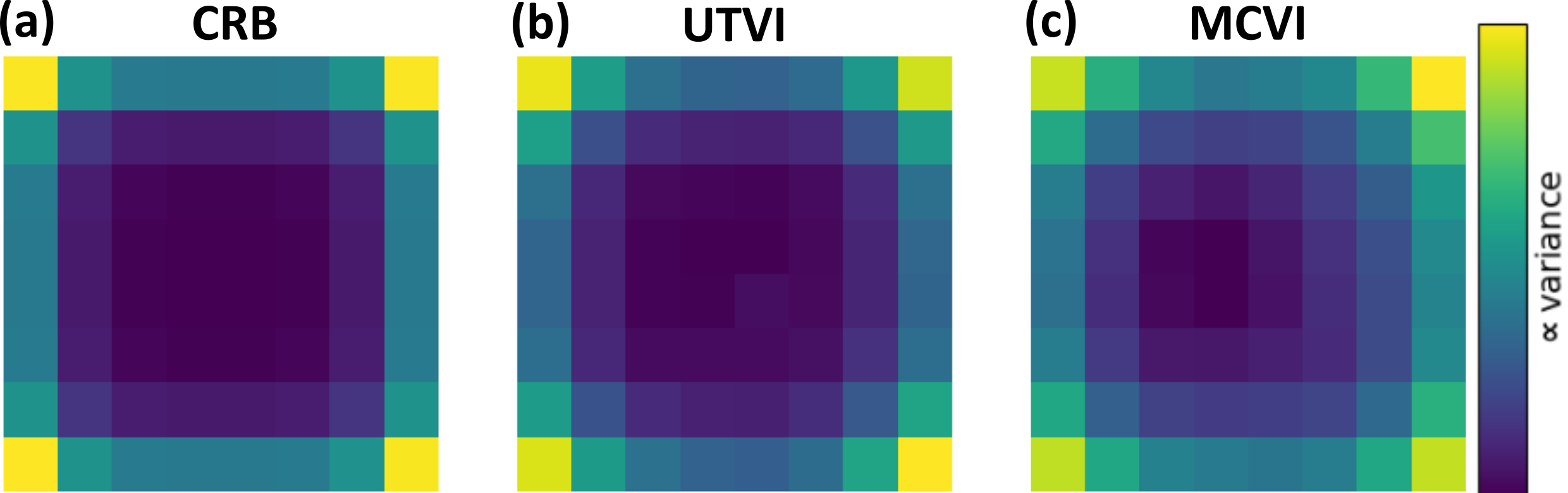
Figure 3: UTVI accurately predicts variance after nonlinear transformation. (a) CRB (Eqn. 6) of emitter position estimates as a function of position across $L\times L$ image. (b-c) Predictive variance of the position inferred by (b) UTVI with 3 sigma points and (c) MCVI with 10 samples for the network architecture described in Section 4.3.3. Images are scaled independently such that color is proportional to variance.

5 Conclusions

In this work, we demonstrated that the unscented transform is an effective and efficient method for propagating the mean and variance through arbitrary nonlinear layers of BNNs, enabling few-sample variational inference of BNNs with an approximately 10X reduced cost as compared to Monte Carlo moment propagation. We have shown that the unscented transform can be used to extend the analytical moment propagation methods of [7, 8, 9] to networks where closed-form moment propagation rules are unavailable or intractable. Additionally, we presented a novel nonlinear activation motivated by inverse transform sampling whose usage in BNNs is enabled or otherwise greatly simplified by our proposed few-sample inference scheme. In summary, we have presented a novel approach to variational inference of BNNs that is simple to implement, computationally efficient, and extensible to arbitrary nonlinear BNN layers.

Appendix A Supplemental figures

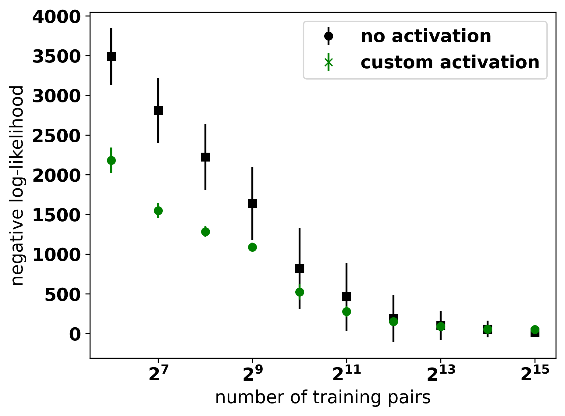
Figure 6: Custom activations improve network generalization. Minimum negative log-likelihood achieved during training over an unseen evaluation set when using no output node activation (black squares) versus the physics-informed activations described in Section 4.3.2 (green dots). Points represent the mean over 10 models trained independently on the same data starting from different random initializations, while error bars represent the standard deviation over the 10 models.

References

- [1] David J. C. MacKay. A Practical Bayesian Framework for Backpropagation Networks. Neural Computation, 4(3):448–472, May 1992.
- [2] Radford M. Neal. Bayesian Learning for Neural Networks, volume 118 of Lecture Notes in Statistics. Springer New York, New York, NY, 1996.
- [3] Geoffrey E Hinton and Drew Van Camp. Keeping the neural net- works simple by minimizing the description length of the weights. In Advances in Neural Information Processing Systems. Proceedings of the sixth annual conference on Computational learning theory, 1993.
- [4] David Barber and Christopher M. Bishop. Ensemble learning in bayesian neural networks. 1998.
- [5] Alex Graves. Practical variational inference for neural networks. In Advances in Neural Information Processing Systems, volume 24. Curran Associates, Inc., 2011.
- [6] Charles Blundell, Julien Cornebise, Koray Kavukcuoglu, and Daan Wierstra. Weight Uncertainty in Neural Networks, May 2015. arXiv:1505.05424 [cs, stat].
- [7] Anqi Wu, Sebastian Nowozin, Edward Meeds, Richard E. Turner, José Miguel Hernández-Lobato, and Alexander L. Gaunt. Deterministic Variational Inference for Robust Bayesian Neural Networks, March 2019. arXiv:1810.03958 [cs, stat].
- [8] Manuel Haußmann, Fred A. Hamprecht, and Melih Kandemir. Sampling-free variational inference of bayesian neural networks by variance backpropagation. In Proceedings of The 35th Uncertainty in Artificial Intelligence Conference, volume 115 of Proceedings of Machine Learning Research, pages 563–573. PMLR, 22–25 Jul 2020.
- [9] David J. Schodt, Ryan Brown, Michael Merritt, Samuel Park, Delsin Menolascino, and Mark A. Peot. A framework for variational inference of lightweight bayesian neural networks with heteroscedastic uncertainties. 2024. arXiv:2402.14532 [cs].
- [10] Simon J. Julier and Jeffrey K. Uhlmann. New extension of the Kalman filter to nonlinear systems. In Ivan Kadar, editor, Signal Processing, Sensor Fusion, and Target Recognition VI, volume 3068, pages 182 – 193. International Society for Optics and Photonics, SPIE, 1997.
- [11] Donald Ebeigbe, Tyrus Berry, Michael M. Norton, Andrew J. Whalen, Dan Simon, Timothy Sauer, and Steven J. Schiff. A generalized unscented transformation for probability distributions. 2021. arXiv:2104.01958 [stat].
- [12] Ilya Loshchilov and Frank Hutter. Decoupled Weight Decay Regularization, January 2019. arXiv:1711.05101 [cs, math].
- [13] Keith A. Lidke, Bernd Rieger, Thomas M. Jovin, and Rainer Heintzmann. Superresolution by localization of quantum dots using blinking statistics. Opt. Express, 13(18):7052–7062, Sep 2005.
- [14] Eric Betzig, George H. Patterson, Rachid Sougrat, O. Wolf Lindwasser, Scott Olenych, Juan S. Bonifacino, Michael W. Davidson, Jennifer Lippincott-Schwartz, and Harald F. Hess. Imaging intracellular fluorescent proteins at nanometer resolution. Science, 313(5793):1642–1645, 2006.
- [15] Michael J Rust, Mark Bates, and Xiaowei Zhuang. Sub-diffraction-limit imaging by stochastic optical reconstruction microscopy (STORM). Nature Methods, 3(10):793–796, October 2006.
- [16] Bo Zhang, Josiane Zerubia, and Jean-Christophe Olivo-Marin. Gaussian approximations of fluorescence microscope point-spread function models. Appl. Opt., 46(10):1819–1829, Apr 2007.
- [17] Raimund J. Ober, Sripad Ram, and E. Sally Ward. Localization accuracy in single-molecule microscopy. Biophysical Journal, 86(2):1185–1200, 2004.