Solving Sequential Manipulation Puzzles by Finding Easier Subproblems

Abstract

We consider a set of challenging sequential manipulation puzzles, where an agent has to interact with multiple movable objects and navigate narrow passages. Such settings are notoriously difficult for Task-and-Motion Planners, as they require interdependent regrasps and solving hard motion planning problems.

In this paper, we propose to search over sequences of easier pick-and-place subproblems, which can lead to the solution of the manipulation puzzle. Our method combines a heuristic-driven forward search of subproblems with an optimization-based Task-and-Motion Planning solver. To guide the search, we introduce heuristics to generate and prioritize useful subgoals. We evaluate our approach on various manually designed and automatically generated scenes, demonstrating the benefits of auxiliary subproblems in sequential manipulation planning.

I Introduction

Manipulation planning in the presence of movable objects and an obstructed environment is challenging: the number of possible action sequences grows with the number of objects, leading to a hard combinatorial problem, whereas obstacles and narrow passages make motion planning difficult. Sequential manipulation requires reasoning about what objects to interact with, how to grasp, and where to place them. At the same time, collision constraints with the environment may introduce interdependencies between grasps, placements of objects, and robot trajectories, making planning especially hard.

Consider the puzzle in Fig. 1, where the 2-DoF robot agent (the yellow circle) has to move the blue cube into the red goal area. Due to the narrow entrances the cube can only be retrieved from behind the wall if the agent grasps it from the bottom or the top, which is not possible at the current position. Multiple regrasps are necessary to solve this problem: e.g. move the cube inside the left entrance (1(b)-1(d)), regrasp from the bottom (1(e)), move to the center (1(f)), regrasp and move to the goal (1(g)-1(h)).

As shown on this example, solving such sequential manipulation problems requires regrasping an object at different angles and positions, finding good intermediate placements for the objects, and planning trajectories. Such problems can be formulated as Task and Motion Planning. However, they pose the following challenges to TAMP planners:

• Motion planning with spatial non-convexities is a challenging problem by itself.

• For optimization-based TAMP approaches the non-convexity could lead to local optima.

• Manipulation planning is especially hard for narrow passages, where only very few grasp positions and orientations lead to feasible downstream paths and manipulation.

To address these challenges, we propose to solve the full TAMP problem by searching sequences of auxiliary pick-and-place subproblems, where objects need to be placed at intermediate locations: the subgoal locations. We introduce heuristics to guide the subproblem search and present several methods to generate subgoals for the pick-and-place subproblems. We evaluate their performance and capability to handle scenes with obstacles and narrow passages.

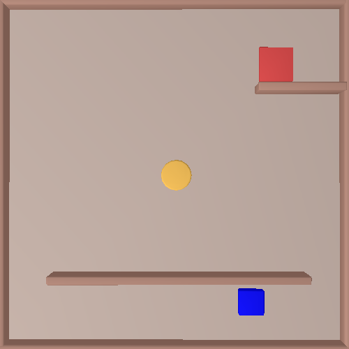
(a)

(b)

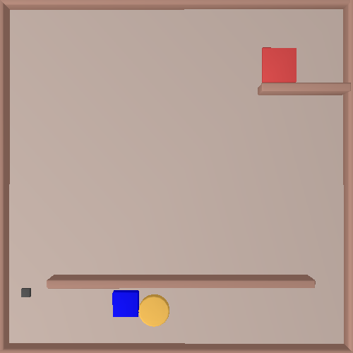
(c)

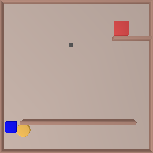
(d)

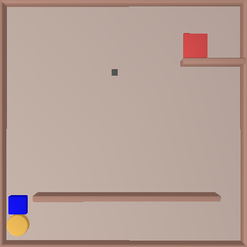
(e)

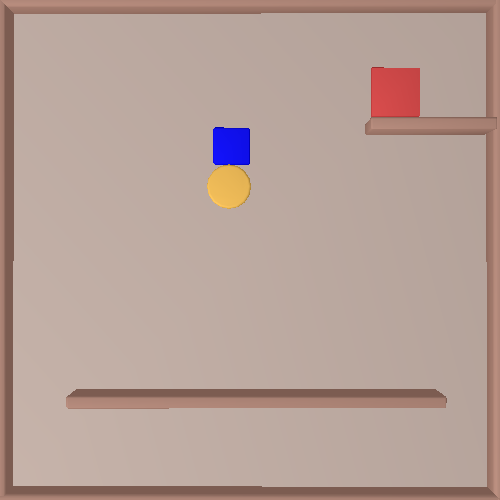
(f)

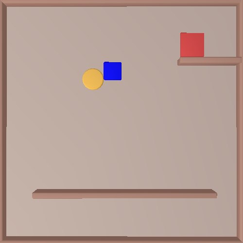
(g)

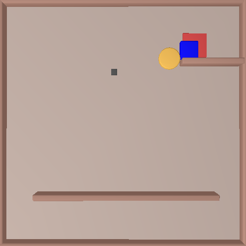
(h)

Figure 1: Solving the Wall pick-and-place puzzle with subgoals. In order to bring the goal-object (blue) to the goal (red square), the agent (yellow circle) moves it and regrasps at several intermediate subgoal locations (gray dots).

To summarize the contributions of our work, in this paper we present:

• A forward search method for solving sequential manipulation problems, integrating a subproblem search with an optimization-based TAMP solver.

• Two approaches to generate and select subgoal locations that serve as regrasp location candidates in a sequential manipulation problem.

• Heuristics to find configurations feasible for the optimization-based TAMP solver and useful to reach the goal.

• A set of pick-and-place puzzles which we created to evaluate our solver, together with solutions and performance metrics.

II Related Works

Many challenges of our problem setting are inherent to Task-and-Motion Planning (TAMP) problems due to the dependencies between discrete logical decisions and continuous physical states. Recent TAMP approaches are thoroughly reviewed in [1]. TAMP solvers differ especially in the way physical constraints and motion planning are integrated into the task planning. Sample-based TAMP planners incrementally discretize the continuous configuration space. For instance, PDDL-Stream [2], combines sequential constrained sampling with PDDL Planning, whereas [3] integrates precomputed samples of feasible configurations into task planning.

Using constraint propagation techniques, physical constraints can be incorporated in task planning to allow informed decisions [4, 5, 6]. Another approach to solve TAMP problems, instead of sampling, is to use optimization methods to resolve dependencies and plan with nonlinear and geometric constraints [7, 8, 9]. Most TAMP solvers focus on long-term planning for manipulating multiple objects in a static environment with few environment constraints, such as placing objects on big tables, with informative goals or task descriptions. In contrast, our problems require shorter action sequences with very precise manipulation, removing potential obstacles, and navigating narrow passages, without any guidance from the symbolic goal. We extend the optimization-based TAMP solver in [7] with a forward search over smaller subproblems, which can be solved with a sampling based motion planner.

Closely related to TAMP, multi-modal planning defines manipulation planning as a hybrid planning with grasps seen as modes [10, 11, 12, 13]. To handle manipulation in constrained spaces, [14] explores the idea of probabilistic roadmaps for planning of grasps and placements. However, they only consider a single movable objects and do not include symbolic task planning. Similarly related is rearrangement planning, addressed by [15, 16, 17, 18], with the important distinction that we do not know the target positions of any additional objects.

The problem settings closest to ours are Manipulation Among Movable Obstacles[19, 20] and Navigation Among Movable Obstacles[21], which can also be considered a special case of TAMP. These approaches often assume monotone manipulation cases, where every object is grasped only once. Many cluttered settings, including some of our puzzles, require multi-step interactions and finding intermediate positions for objects, before moving them to the goal.

The concept of subgoals has been extensively discussed in Reinforcement Learning (RL), e.g. [22, 23, 24, 25]. While these works do not address TAMP, they provide interesting ideas for proposing subgoals. In particular, diverse density analysis [26] is an approach to characterize bottleneck regions, on which our method builds to propose subproblems.

In classical planning, landmarks [27], (related to our definition of subgoals) are used to guide search-based planning [28, 29], but are defined in the discrete logic domain. We draw on such ideas and transfer them to proposing manipulation subproblems for TAMP solving.

III Problem Formulation and Notation

III-A Logic Geometric Programming for TAMP

We adopt an optimization-based formulation of Task-and-Motion Planning, namely as Logic-Geometric Program (LGP)[7][30]. Given the configuration space ${\mathcal{X}}={\mathbb{R}}^{n}\times SE(3)^{m}$ of a $n$-DoF robot and $m$ movable objects, LGP assumes that feasible paths are structured in phases (or modes), where smooth differentiable constraints describe the feasible motions in each mode and feasible transitions (switches) between modes, akin to multi-modal path planning [10]. A Logic-Geometric Program is a nonlinear mathematical program (NLP) of the form

$$\min_{K,s_{1:K}\atop x:[0,t_{K}]\to{\mathcal{X}}}~{} \int^{t_{K}}_{0}c(\bar{x}(t))~{}dt$$ (1a)

s.t. $$~{}~{}~{}~{}~{}~{}~{}~{}x(0)=x_{0},~{}~{}~{}~{}\,h_{\text{goal}}(x(t_{K}))\leq 0,$$ (1b)

$$\forall_{k}:\forall_{t}\in[t_{k{\text{-1}}},t_{k}]:h_{\text{mode}}(\bar{x}(t),s_{k})\leq 0,$$ (1c)

$$~{}~{}~{}~{}~{}~{}~{}~{}~{}~{}~{}~{}~{}~{}~{}\,h_{\text{switch}}(\bar{x}(t_{k}),s_{k{\text{-1}}},s_{k})\leq 0,$$ (1d)

$$\forall_{k}:s_{k}\in\text{succ}(s_{k{\text{-1}}}),~{}s_{K}\models\mathfrak{g}$$ (1e)

where $\bar{x}(t)=(x(t),\dot{x}(t),\ddot{x}(t))$. The decision variables of this NLP are the number of phases $K$, the symbolic mode sequence $s_{1:K}$, and the continuous path $x(t)$. The path is constrained to start at $x_{0}$ and end in a configuration $x(t_{K})$ consistent with the goal constraints $h_{\text{goal}}$. In each phase, the path needs to fulfill mode constraints $h_{\text{mode}}$ depending on the symbolic mode $s_{k}$, and each $\bar{x}(t_{k})$ needs to fulfill mode-switch constraints $h_{\text{switch}}$ depending on the symbolic mode transition. The times $t_{k}$ of mode transitions are assumed to be fixed and equal spaced. Only certain mode transitions are possible logically, here notated via a successor function (usually given as a STRIPS-like task planning domain[31]). Finally, $\mathfrak{g}$ denotes a logical goal. All constraint functions $h$ are assumed smoothly differentiable, and are here written as inequalities – but this is meant to also include equality constraints which an NLP solver handles differently.

III-B Problem Formulation

The LGP (1) is a very general formulation for TAMP. In this work, we consider a subclass of problems where the available discrete actions are restricted to pick and place of any object $o_{m}$ in the scene using a stable grasp and placement on the ground. In all problems, the goal $\mathfrak{g}$ is to put the goal object $o_{\textit{goal}}\in\mathcal{O}$ on the red goal surface $goal$. We define this problem as $\mathcal{P}(x_{0},\mathfrak{g})$ for initial configuration $x_{0}\in{\mathcal{X}}$.

We consider sequential manipulation problems requiring multiple regrasps, moving away objects and moving objects through tight spaces. However, $\mathfrak{g}$ does not contain any information to plan these manipulations, grasps and movements. Our approach is to find and solve auxiliary subproblems, which will guide our planner over a sequence of subgoals to a configuration $x_{\text{feas}}$ from which $\mathfrak{g}$ can be solved.

III-C Pick-and-Place Auxiliary Subproblems

Starting from a configuration $x_{i}\in{\mathcal{X}}$, the pick-and-place auxiliary subproblem $\mathcal{\tilde{P}}(x_{i},g)$ is defined as the task of moving an object $o\in\mathcal{O}$ to a position $z\in SE(3)$ in a single pick-and-place sequence, with $g$ being the object-position tuple $(o,z)$ and defined as a subgoal.

$\mathcal{\tilde{P}}$ is an instance of an LGP problem with two phases $K=2$ and a fixed sequence of mode-transitions: $(\texttt{pick}~{}o_{1})$, $(\texttt{place}~{}o_{1}~{}\texttt{in}~{}z)$. To pick an object, the robot should be able to touch it, with grasps possible from all angles. Once picked, the object is attached with a rigid joint until it is placed in $z$. The poses for pick and place are optimized jointly for the following constraints. The goal constraint $h_{\text{goal}}$ is a pose constraint depending on $z$. The switch constraints $h_{\text{switch}}$ are touch and stable for pick, and above and stable-on for the place action as defined in [30].

The solution of a subproblem $\mathcal{\tilde{P}}(x_{i},g)$ is a collision-free path $X$ from $x_{i}=X(0)$ to a final configuration $x^{f}=X(T)$ that meets the subgoal $g$. We use the following notation to indicate feasibility of a subproblem and return the final configuration:

$$x^{f}=\text{solve}~{}\mathcal{\tilde{P}}(x_{i},g),$$ (2)

The configuration $x^{f}$ is a valid configuration that can be used later as a start for the original problem $\mathcal{P}(x^{f},\mathfrak{g})$ or subsequent subproblems.

III-D Subproblem Sequence

To solve the original problem (1), we aim to find a sequence of subgoals $[g_{1},\ldots,g_{L}]$ such that,

$$x^{f}_{0}\equiv x_{0},$$ (3)

$$\forall_{i\in[1,...,L]}:x^{f}_{i}=\text{solve}~{}\mathcal{\tilde{P}}(x^{f}_{i-1},g_{i}),$$ (4)

$$~{}~{}~{}~{}~{}~{}~{}~{}~{}~{}~{}~{}x_{\text{goal}}=\text{solve}~{}\mathcal{P}(x^{f}_{L},\mathfrak{g})~{}.$$ (5)

The sequence of subproblems is represented as a graph in Fig. 2, which starts at node $x_{0}$, and is expanded using new subproblems (e.g. $\mathcal{\tilde{P}}(x_{0},g_{0})$ and $\mathcal{\tilde{P}}(x_{0},g_{1})$) or the original problem $\mathcal{P}(x_{0},\mathfrak{g}$). The solid edges represent solution paths, leading to new valid configurations. Once $\mathcal{P}$ is solved for $\mathfrak{g}$, we can trace the complete solution from $x_{0}$ to $x_{\text{goal}}$.

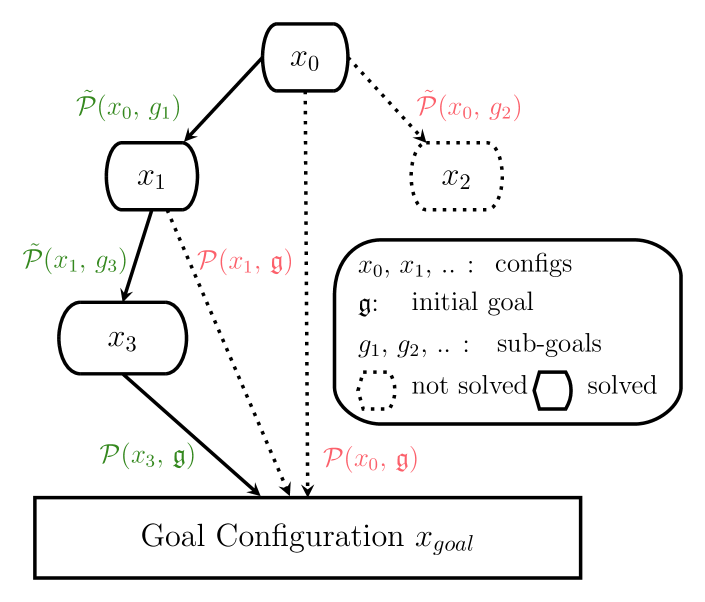
Figure 2: Subproblem sequence. Solved subproblems and problems in green, unsolved in red.

IV Solving Multi-Step Manipulation Problems using a Sequence of Subgoals

The main idea of our method is to perform a forward search over possible pick-and-place subproblems $\mathcal{\tilde{P}}$ to reach a configuration $x_{f}$, for which we can solve the original problem $\mathcal{P}(x_{f},\mathfrak{g})$. We cannot derive such subproblems directly from the goal, because the symbolic goal only defines constraints on one object ($o_{goal}$) and these constraints are only related to its final position. Most importantly, the goal does not provide information on whether we need to move other objects, in what order or over which trajectories. Instead, we introduce heuristics in our search algorithm to come up with helpful and solvable subproblems.

In Alg. 1 we outline the main steps of our approach. At every iteration of the main loop, we select one of the configurations $x$ from the list $L$ using feasibility heuristics in select_node. We try to solve the original problem $\mathcal{P}(x,\mathfrak{g})$ with solve, which uses Multi-Bound Tree Search (MBTS)[32], which is a solver for LGP. It explores possible sequences of discrete actions using a tree search algorithm with multiple geometric bounds. These bounds allow to quickly test the feasibility of path and mode-switch configurations in (1) for a fixed action skeleton by solving informative relaxations of the trajectory optimization problem. If successful, solve returns a path $X$.

If $\mathcal{P}(x,\mathfrak{g})$ was not solved, we try to reach configurations from which it may be solvable. We generate subgoals for objects reachable to the agent using propose_subgoals, giving us a set of auxiliary pick-and-place subproblems $\mathcal{\tilde{P}}$. In comparison to the original problem $\mathcal{P}$, solving $\mathcal{\tilde{P}}$ does not require a search over different discrete actions. We solve the auxiliary subproblems using a fixed-action-sequence solver sub_solve: a combination of nonlinear optimization and sample based motion planning. First, we compute the mode-switch configurations for the grasp and the placement of the object using nonlinear optimization with a randomized initialization. Second, we use bi-directional Rapidly-exploring Random Trees (RRTs) [33], to compute a collision-free path between the mode-switch configurations, similar to [34].

The solutions of $\mathcal{\tilde{P}}$ give us trajectories leading to new valid configurations, which are added to the list L of start configurations to try. The search concludes, if either we solve $\mathcal{P}$ or we do not have any more configurations to expand.

Algorithm 1 Forward subproblem search

1:Input: Start configuration $x_{0}$, logical goal $\mathfrak{g}$

2:$L\leftarrow\{x_{0}\}$ $\triangleright$ Initialize list of valid configurations

3:while $L$ not empty do

4:     $x\leftarrow\texttt{select\_node}(L)$ $\triangleright$ s. IV-A

5:     $X\leftarrow\texttt{solve}~{}\mathcal{P}(x,\mathfrak{g})$ $\triangleright$ Try to reach goal

6:     if $X$ found then

7:         Return $X_{\text{full}}$ $\triangleright$ Trace solution back to $x_{0}$      

8:     for $o\in\mathcal{O}$ do

9:         if not reachable($x$, $o$)  then

10:              Continue          

11:         $Z\leftarrow\texttt{propose\_subgoals}(x,o)$ $\triangleright$ s. IV-B

12:         for $z\in Z$ do

13:              $g\leftarrow(o,z)$ $\triangleright$ New subgoal $g$

14:              $X\leftarrow\texttt{sub\_solve}~{}\mathcal{\tilde{P}}(x,g)$

15:              if $X$ found and not rej($L$, $x^{f}$) then

16:                  $\texttt{Insert}(L,x^{f})$ $\triangleright$ add last element of $X$                             

17:Return None $\triangleright$ No solution found

IV-A Prioritizing configurations with select_node

Intuitively, we would like to prioritize configurations from which the LGP-Solver is more likely to solve the problem $\mathcal{P}$. We introduce the score function $s(x)=10v_{o}+5v_{g}+v_{\text{dist}}$ to select configurations, where

• $v_{o}$ is 1, if there is a line-of-sight between $o_{\text{goal}}$ and the goal, and 0 otherwise.

• $v_{g}$ is 1, if there is a line-of-sight between $o_{\text{goal}}$ and the agent, and 0 otherwise.

• $v_{\text{dist}}$ measures proximity $d$ of $o_{\text{goal}}$ to the goal, and is set to 5 if $d<0.2$, 2 if $d<0.4$, and 0 otherwise.

We only expand a configuration twice, if all other configurations in $L$ have been tried. If every configuration has been tried twice, we stop the search.

IV-B Generating Subproblems with propose_subgoals

First, to decide on the object $o$, we try to find a collision-free path to the object center with bi-directional RRT to check if the object is reachable to the agent. Hard to reach objects can still be deemed unreachable, as we limit the RRT step budget.

Second, for a given object $o$ we generate a set of subgoal positions $Z$ with the propose_subgoals method:

1. Generate position candidates.

2. Filter candidates with Filter (see IV-B1).

3. From the filtered positions sample a small subset ($Z$).

We evaluated several methods to generate the initial subgoal positions:

• Rnd: randomly generated

• Btl: using bottleneck analysis

• Hum: from human demonstrations

Btl: to find optimal subgoal positions we look for bottlenecks in the scene, i.e. entrances or narrows passages you need to pass to reach other areas. Similar to diverse density analysis in [26], we look for areas with a higher number of possible paths leading through them. First, we rasterize the scene and construct a grid-like graph, with vertices connected only if there is a path between them for the object $o$. Then we calculate the shortest paths from vertices in a small area around the current object to all other vertices in the graph. We use the number of paths passing through a vertex relative to the number of vertices as a measure of paths density of this vertex. Compared to random sampling, the Btl method is far more likely to propose a position inside a narrow space than inside a larger area, which helps to guide the subgoal generation to the bottlenecks.

IV-B1 Filtering subgoal positions with Filter

from the set of generated positions, we select the most promising ones with heuristics from IV-A: we calculate the feasibility score of a hypothetical solution configuration, assuming the object $o$ was successfully moved to the subgoal position $z$. Then we filter the positions based on their scores. Filtering helps to find positions, where $o_{goal}$ would be either close to the $goal$ or in line-of-sight of it. A distribution of the subgoal positions before and after filtering is visualized in Fig. 3.

Finally, from the filtered positions we randomly sample a subset of subgoals, adding a trivial subgoal, where the position is equal to the current position of the object.

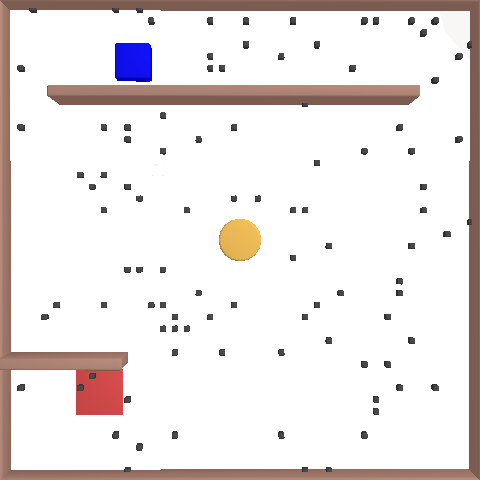
(a)

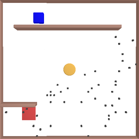
(b)

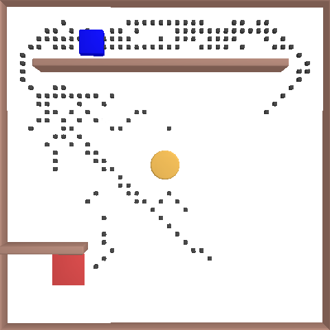
(c)

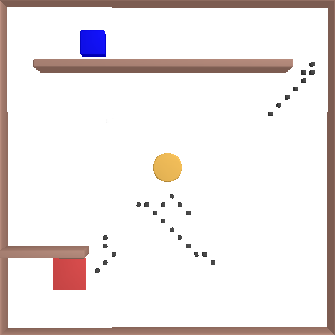
(d)

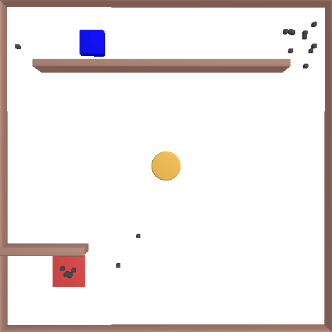
(e)

Figure 3: Subgoals in the scene Wall. a) Rnd b) Rnd filtered by heuristics. c) Btl d) Btl after filtering e) Hum

IV-C Rejecting similar configurations with rej

After a subproblem is solved, we add the last configuration of the solution path to the list $L$. To avoid repeating problems, we calculate a similarity value for configurations, based on the discretized positions of movable objects, and allow at most two similar configurations to be added.

V Experiments

We evaluated the solver on pick-and-place puzzles of different complexity, addressing common TAMP challenges. While we formulated our problem in a general way with object poses in $SE(3)$, we consider a robot with 2-DoF to highlight the challenges of interdependencies between grasps and trajectories. Our benchmark problems include:

• 9 manually designed puzzles, challenging for the solver due to multiple obstacles and bottlenecks, Fig. 4.

• 360 PCG (Procedural Content Generation) scenes: automatically generated maze-style puzzles with two objects, allowing us to evaluate how well the approach performs in general settings, Fig. 5.

To create the PCG scenes, we used the PCGRL Framework, which can generate solvable gridworld game levels of varying difficulty[35][36]. We converted the gridworld scenes (Sokoban levels) to continuous 3D TAMP problems.

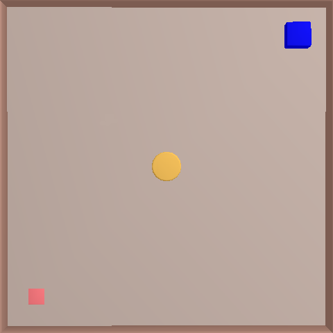
(a)

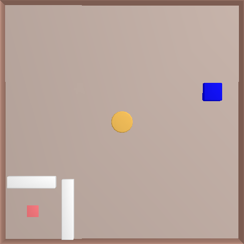
(b)

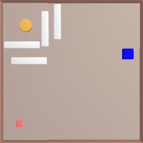
(c)

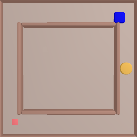
(d)

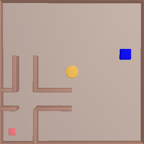
(e)

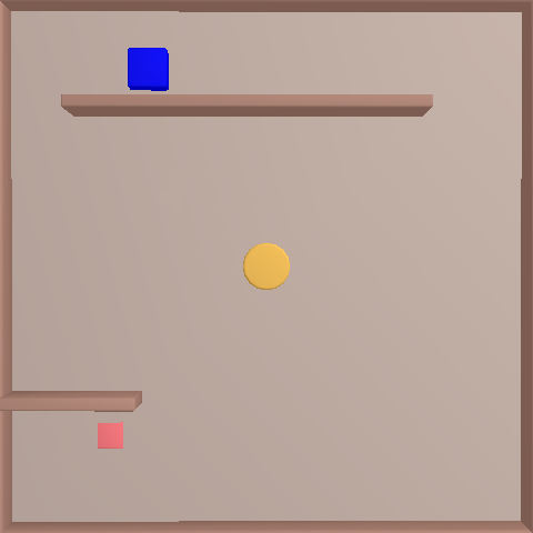
(f)

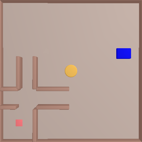
(g)

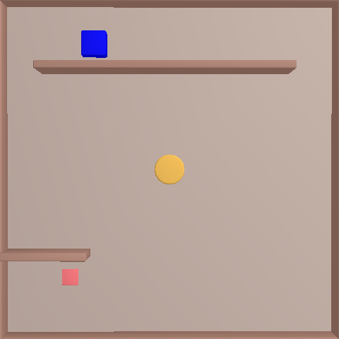
(h)

Figure 4: Puzzle scenes: the agent (yellow circle) needs to bring the goal-object (blue) to the goal (red square). Movable obstacles in white, static walls in brown.

We measured the following metrics:

1. Completeness: solution ratio over multiple runs.

2. Performance: solution time.

3. Success rate: percentage of solved PCG scenes.

The performance and completeness experiments are repeated 10 times on 9 manually designed puzzles and 12 PCG problems. In Table I we report the solution times, the standard deviation and the solution rate, if it is below 100%. We used a single i7-11700@2.5 GHz CPU for the tests. The success rate experiments are repeated once on all PCG problems and we count the number of solved problems.

We compared three methods to generate subgoals (s. IV-B): Rnd, Btl, and Hum. Using random subgoals Rnd, we evaluated the importance of the individual components:

• F - Filter, heuristics based filtering of subgoals during subgoal generation, s. Filter in IV-B1.

• P - Prio: heuristics based selection of next configurations for node expansion in select_node.

• R - Reject: diversity based rejection of new configurations from solved subproblems.

In total, we evaluated the following combinations of methods (as reported in Tab. I):

1. Rnd+FPR: the full method with random subgoals (Filter: yes, Prio: yes, Reject: yes).

2. Rnd+FP: without rejection of similar configrations (Filter: yes, Prio: yes, Reject: no).

3. Rnd+FR: without heuristics for configuration prioritization (Filter: yes, Prio:no, Reject: yes)

4. Rnd+R: without heuristics (Filter: no, Prio: no, Reject: yes).

5. Btl+FPR: subgoals from the bottleneck analysis, (Filter: yes, Prio: yes, Reject: yes)

6. Hum+R: manual subgoals, without heuristics (Filter: no, Prio: no, Reject: yes)

7. MBTS: baseline method, Multi-Bound Tree Search.

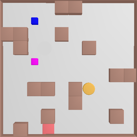
(a)

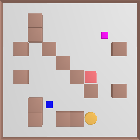
(b)

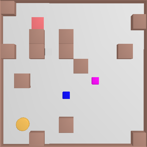
(c)

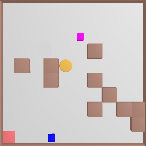
(d)

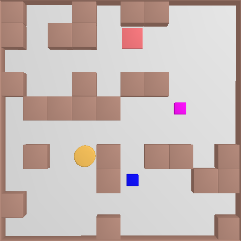
(e)

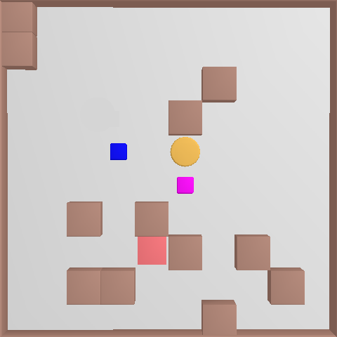
(f)

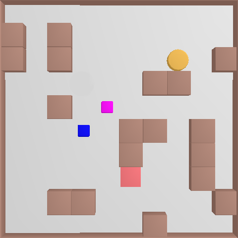
(g)

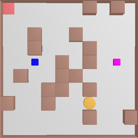
(h)

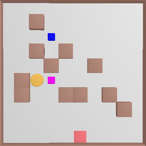
(i)

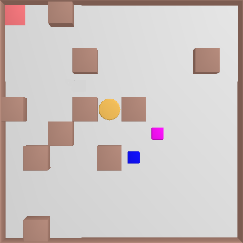
(j)

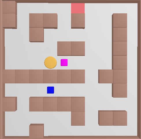
(k)

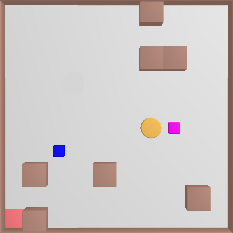
(l)

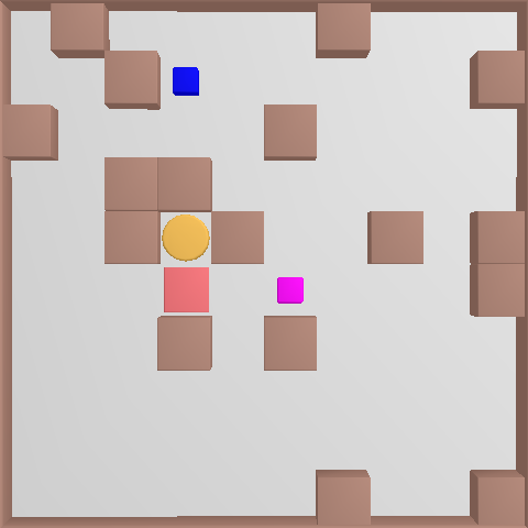
(m)

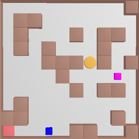
(n)

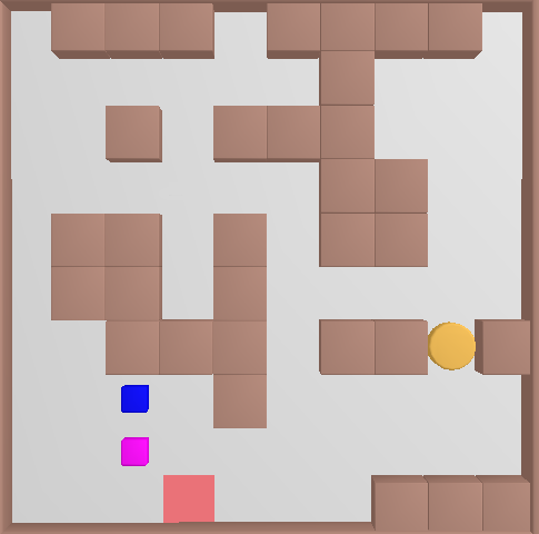
(o)

Figure 5: Proceduraly Generated Scenes (subset) with walls (brown) and two movable objects: the goal-object (blue) and an obstacle-object (pink).

VI Results

TABLE I: Average solution time over 10 runs (s). Rnd: random subgoals, Btl: bottleneck subgoals, Hum: subgoals from human demonstrations.  Ablations: Rnd+FP: no rejection of similar configs, Rnd+FR: no heuristics to select next config, Rnd+R: no heuristics. Solution rate in percent, if below 100% and ’-’, if not solved. For Btl+FPR: in square brackets the time without computing subgoals.

Scene	Rnd+FPR	Rnd+FP	Rnd+FR	Rnd+R	Btl+FPR	Hum+R	MBTS
Cube-Free	0.2$\pm$0.01	0.2$\pm$0.01	0.2$\pm$0.01	0.2$\pm$0.01	0.2$\pm$0.01		0.2$\pm$0.01
Corner	0.3$\pm$0.01	0.3$\pm$0.01	0.3$\pm$0.01	0.3$\pm$0.01	0.3$\pm$0.01		0.3$\pm$0.01
2 blocks	2.5$\pm$0.01	2.6$\pm$0.01	2.5$\pm$0.01	2.5$\pm$0.04	2.5$\pm$0.01		2.5$\pm$0.02
4 blocks	38.4$\pm$23.01	35.2$\pm$20.57	41.7$\pm$15.45	30.4$\pm$23.22	165.8$\pm$81.87[55.8]	176.6$\pm$68.29	-
Maze-Easy	54.0$\pm$10.96	56.0$\pm$10.91	84.7$\pm$38.45	155.4$\pm$86.73	143.9$\pm$94.29[85.7](80.0%)	55.2$\pm$9.27	-
Wall-Easy	1.8$\pm$0.16	2.1$\pm$0.29	7.8$\pm$9.89	9.4$\pm$8.73	8.3$\pm$2.19[2.4]	3.5$\pm$4.45	-
O-Room	68.3$\pm$56.10	100.7$\pm$80.62	92.9$\pm$76.65	254.5$\pm$170.08	259.2$\pm$128.40[102.6]	61.1$\pm$30.37	-
Maze	926.2$\pm$615.78	1750.7$\pm$1075.61(90.0%)	1454.8$\pm$1133.81	2867.7$\pm$1781.67(40.0%)	1772.5$\pm$1319.81[839.4](80.0%)	154.9$\pm$162.50(80.0%)	-
Wall	190.1$\pm$130.60	125.6$\pm$111.11	240.0$\pm$108.18	91.8$\pm$84.86	59.7$\pm$25.21[32.6](90.0%)	55.9$\pm$41.72	-
a11-6	33.4$\pm$9.71	31.6$\pm$4.61	56.3$\pm$35.00	123.8$\pm$94.97	67.7$\pm$21.98[33.1]		-
a15-20	11.2$\pm$1.08	12.0$\pm$3.19	18.7$\pm$9.77	57.2$\pm$44.36	42.0$\pm$15.49[14.2]		-
a19-20	0.4$\pm$0.01	0.4$\pm$0.01	0.3$\pm$0.01	0.3$\pm$0.01	0.3$\pm$0.01		0.4$\pm$0.01
a22-4	45.9$\pm$0.22(20.0%)	46.7$\pm$0.32(20.0%)	147.7$\pm$91.98	120.9$\pm$66.96	170.5$\pm$54.49[81.4](30.0%)	144.4$\pm$72.16	-
a23-78	13.9$\pm$5.03	22.5$\pm$27.59	48.5$\pm$56.25	135.1$\pm$100.35	60.2$\pm$28.71[22.4]		-
a29-0	31.9$\pm$18.89	29.2$\pm$5.11	28.1$\pm$11.44	47.1$\pm$34.09	46.7$\pm$1.95[22.5]		-
a35-2	9.8$\pm$2.32	10.6$\pm$1.75	14.3$\pm$8.99	60.9$\pm$55.65	55.5$\pm$24.94[17.6]		-
a3-92	30.2$\pm$21.01	29.3$\pm$32.81	46.3$\pm$23.11	99.4$\pm$70.47	48.2$\pm$22.97[20.0]	62.9$\pm$76.90	-
a5-43	21.1$\pm$5.47	29.3$\pm$24.47	41.0$\pm$16.94	67.3$\pm$35.52	36.6$\pm$7.27[16.5]		-
a19-18	15.7$\pm$4.15	14.2$\pm$5.41	21.4$\pm$11.76	47.1$\pm$28.99	42.1$\pm$23.61[16.7]		-
a23-6	73.1$\pm$42.11	61.6$\pm$39.50	148.3$\pm$102.77	86.9$\pm$47.62	84.4$\pm$35.56[37.4]	69.8$\pm$60.94	-
a31-4	22.0$\pm$3.86	24.0$\pm$12.99	25.2$\pm$12.94	43.1$\pm$15.09	50.8$\pm$3.41[20.5]		-

Comparison to the MBTS Baseline: Table I summarizes the results of our evaluations. We find that our method (Rnd+FPR) consistently solves the benchmark problems while the baseline solver (MBTS) fails (dashes) at problems with objects hidden behind walls and narrows passages (e.g. Maze, Maze-Easy, O-Room). As our method tries direct MBTS first, the runtimes for solved problems are the same.

We further analyzed the success rate over all 360 PCG problems and found 99.7% for Rnd+FPR vs 73.6% for MBTS. The improvement is especially visible for problems where $o_{\text{goal}}$ is behind obstacles: in 122 out of 360 PCG scenes the $o_{\text{goal}}$ is at least partially occluded from the agent by an obstacle, while the other 238 have no occlusion (direct line-of-sight). With the subgoals search, we can solve 100% of non-occluded and 99.1% of occluded problems. With MBTS 88.24% and 45.08% respectively. The scene a4-2 (Fig. 5(o)) was not solved, as all objects were marked as unreachable.

Comparison of the subgoal generation methods: Table I also reports the results for the three subgoal generation methods described in IV-B in the columns Rnd+FPR, Btl+FPR and Hum+R. Overall, the Rnd+FPR (random subgoals with heuristics) performs better than Btl subgoals in terms of solution time and solution rate for most scenes: it shows faster average time in 16 out of 21 scenes, and similar in 4, and has in all but one scenes 100% solution rate. The observed time difference is mostly due to the overhead to calculate the bottleneck subgoals. However, for scenes Wall and Maze, where the subgoals need to be placed in specific small areas, the Btl and Hum subgoals lead to faster search times (excluding the time to create or generate subgoals), as can be seen in Fig. 6(b).

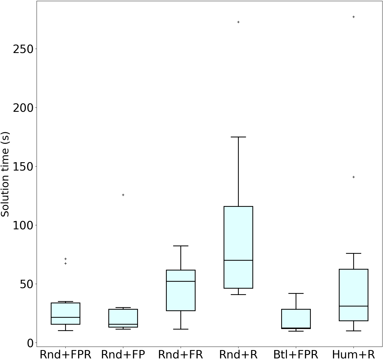
(a) PCG Scene a3-92

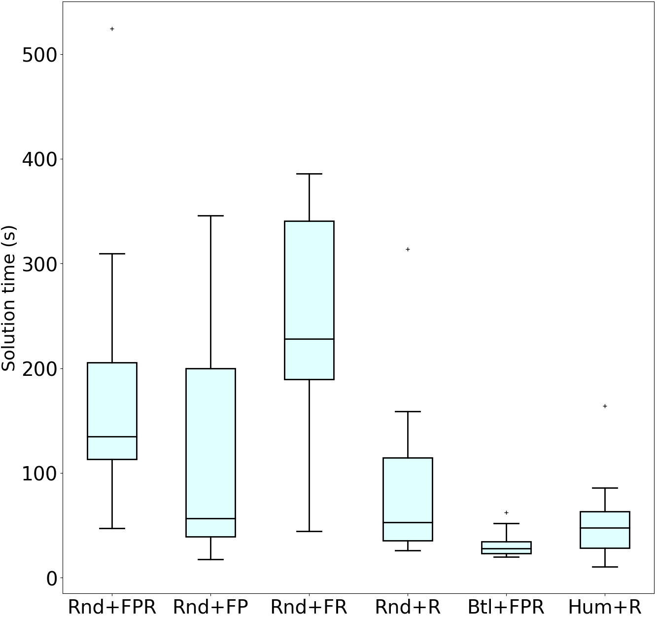
(b) Wall

Figure 6: Runtime comparison over 10 runs (excl. runs without a solution). For Btl: the time without subgoal generation.

Discussion of feasibility heuristics: Filtering subgoals with Filter provides a significant performance boost, as reported in columns Rnd+FR and Rnd+R. While we sample the same amount of subgoals in both methods, with filtering we select subgoal positions with $o_{goal}$ closer to the goal or in line-of-sight of it. However, as seen in Fig. 6, filtering of random subgoals leads to highly varying results in the Wall scene, where success strongly depends on finding the narrow opening, while filtering leaves only few candidates in this area (Fig. 3(b)).

Prioritizing configurations with a higher score, as described in Sec. IV-A, leads to a faster solution in 16 out of 21 scenes, as can be seen on Rnd+FPR and Rnd+FR results of Tab. I and both scenes in Fig. 6.

Rejecting similar configurations: We compare the runtime of the full version Rnd+FPR to the ablation version Rnd+FP, where we do not reject similar configurations. In most scenes the search finishes before we encounter similar configurations, except for Maze, Wall and O-Room, which take longer. For Maze we observed a higher number of rejected configurations in Rnd+FPR, and for this problem the non-rejecting ablation Rnd+FP is slower. However, for the scene Wall, we see the opposite effect in some of the runs, with the lower median time for Rnd+FP (Fig. 6(b)). This indicates that it can be beneficial to try similar configurations for problems, where the objects are initially hard to reach.

Comparison to human-baseline subgoals: Only two scenes (Maze and Wall) significantly benefit from the Hum subgoals, and the scene O-Room is slightly better than Rnd+FPR. These are hard problems with narrow passages, but only a single object without additional obstacles. We conclude that having a good initial guess for the subgoals only helps if the scene remains unchanged and has only few possible solutions. In most other problems (especially 4-blocks and the PCG scenes) the positions of the agent and the objects can be very different in every solution. Therefore, generating subgoals dynamically for every configuration leads to better average performance than having a set of good but fixed subgoals.

VII Conclusions

Integrating subproblem search with a baseline LGP-Solver enables us to plan for scenes which are not feasible for the baseline solver alone: containing occluded objects, obstacles and multiple narrow passages. By using simple heuristics to generate subgoals and select configurations, we can significantly decrease the time to solution. We have shown that our approach is applicable to a wide variety of layouts.

For most scenes, the subgoals generated by the random heuristic lead to similar or better solution rates and times compared to subgoals from human demonstrations. This shows that our approach does not require the subgoals to be in optimal positions, but it benefits from the ability to dynamically generate diverse subgoals. The two scenes (Maze and Wall) where manual subgoals provide an advantage, are also the ones where a bottleneck heuristic performs better.

Our approach results in very interesting puzzle solutions, combining object repositioning, navigating through passages and refined multi-step object interactions. However, the solutions could be potentially optimized in terms of the path lengths or the number of object interactions.

In our evaluations we focused on pick-and-place actions, but the approach is also applicable to other interactions, as pushing.

References

- [1] C. R. Garrett, R. Chitnis, R. Holladay, B. Kim, T. Silver, L. P. Kaelbling, and T. Lozano-Pérez, “Integrated task and motion planning,” arXiv preprint arXiv:2010.01083, 2020.
- [2] C. R. Garrett, T. Lozano-Pérez, and L. P. Kaelbling, “Pddlstream: Integrating symbolic planners and blackbox samplers via optimistic adaptive planning,” in Proceedings of the International Conference on Automated Planning and Scheduling, vol. 30, 2020, pp. 440–448.
- [3] J. Ferrer-Mestres, G. Francès, and H. Geffner, “Combined task and motion planning as classical AI planning,” CoRR, 2017.
- [4] F. Lagriffoul, D. Dimitrov, J. Bidot, A. Saffiotti, and L. Karlsson, “Efficiently combining task and motion planning using geometric constraints,” The International Journal of Robotics Research, 2014.
- [5] J. Bidot, L. Karlsson, F. Lagriffoul, and A. Saffiotti, “Geometric backtracking for combined task and motion planning in robotic systems,” Artificial Intelligence, vol. 247, 05 2015.
- [6] T. Lozano-Pérez and L. P. Kaelbling, “A constraint-based method for solving sequential manipulation planning problems,” in 2014 IEEE/RSJ International Conference on Intelligent Robots and Systems, 2014, pp. 3684–3691.
- [7] M. Toussaint, “Logic-geometric programming: An optimization-based approach to combined task and motion planning,” in International Joint Conference on Artificial Intelligence, 2015.
- [8] J. Ortiz-Haro, E. Karpas, M. Katz, and M. Toussaint, “Conflict-directed diverse planning for logic-geometric programming,” in Proceedings of ICAPS, 2022.
- [9] ——, “A conflict-driven interface between symbolic planning and nonlinear constraint solving,” IEEE Robotics and Automation Letters, vol. 7, no. 4, pp. 10 518–10 525, 2022.
- [10] K. Hauser and V. Ng-Thow-Hing, “Randomized multi-modal motion planning for a humanoid robot manipulation task,” International Journal of Robotics Research, vol. 30, no. 6, pp. 678–698, 2011.
- [11] W. Vega-Brown and N. Roy, “Asymptotically optimal planning under piecewise-analytic constraints,” in Algorithmic Foundations of Robotics XII. Springer, 2020, pp. 528–543.
- [12] Z. Kingston, A. M. Wells, M. Moll, and L. E. Kavraki, “Informing multi-modal planning with synergistic discrete leads,” in IEEE International Conference on Robotics and Automation, 2020, pp. 3199–3205.
- [13] P. S. Schmitt, W. Neubauer, W. Feiten, K. M. Wurm, G. V. Wichert, and W. Burgard, “Optimal, sampling-based manipulation planning,” in 2017 IEEE International Conference on Robotics and Automation (ICRA). IEEE, 2017, pp. 3426–3432.
- [14] T. Siméon, J.-P. Laumond, J. Cortés, and A. Sahbani, “Manipulation planning with probabilistic roadmaps,” International Journal of Robotics Research, vol. 23, no. 7-8, pp. 729–746, 2004.
- [15] J. Ota, “Rearrangement of multiple movable objects - integration of global and local planning methodology,” in IEEE International Conference on Robotics and Automation, 2004. Proceedings. ICRA ’04. 2004, vol. 2, 2004, pp. 1962–1967 Vol.2.
- [16] R. Wang, Y. Miao, and K. E. Bekris, “Efficient and high-quality prehensile rearrangement in cluttered and confined spaces,” in 2022 International Conference on Robotics and Automation (ICRA). IEEE, 2022, pp. 1968–1975.
- [17] K. Ren, P. Chanrungmaneekul, L. E. Kavraki, and K. Hang, “Kinodynamic rapidly-exploring random forest for rearrangement-based nonprehensile manipulation,” in 2023 IEEE International Conference on Robotics and Automation (ICRA). IEEE, 2023, pp. 8127–8133.
- [18] S. B. Bayraktar, A. Orthey, Z. Kingston, M. Toussaint, and L. E. Kavraki, “Solving rearrangement puzzles using path defragmentation in factored state spaces,” IEEE Robotics and Automation Letters, 2023.
- [19] D. M. Saxena, M. S. Saleem, and M. Likhachev, “Manipulation planning among movable obstacles using physics-based adaptive motion primitives,” 2021 IEEE International Conference on Robotics and Automation (ICRA), pp. 6570–6576, 2021. [Online]. Available: https://api.semanticscholar.org/CorpusID:231846605
- [20] M. Stilman, J.-U. Schamburek, J. Kuffner, and T. Asfour, “Manipulation planning among movable obstacles,” in Proc. of the IEEE Int. Conf. on Robotics and Automation (ICRA). IEEE, 2007, pp. 3327–3332.
- [21] M. Stilman and J. J. Kuffner, Planning Among Movable Obstacles with Artificial Constraints. Berlin, Heidelberg: Springer Berlin Heidelberg, 2008, pp. 119–135. [Online]. Available: https://doi.org/10.1007/978-3-540-68405-3˙8
- [22] E. Chane-Sane, C. Schmid, and I. Laptev, “Goal-conditioned reinforcement learning with imagined subgoals,” in International Conference on Machine Learning. PMLR, 2021, pp. 1430–1440.
- [23] S. Nasiriany, V. Pong, S. Lin, and S. Levine, “Planning with goal-conditioned policies,” Advances in Neural Information Processing Systems, vol. 32, 2019.
- [24] F. Xia, C. Li, R. Martín-Martín, O. Litany, A. Toshev, and S. Savarese, “Relmogen: Integrating motion generation in reinforcement learning for mobile manipulation,” in 2021 IEEE International Conference on Robotics and Automation (ICRA), 2021, pp. 4583–4590.
- [25] T. Jurgenson, O. Avner, E. Groshev, and A. Tamar, “Sub-goal trees a framework for goal-based reinforcement learning,” in Proceedings of the 37th International Conference on Machine Learning, ser. Proceedings of Machine Learning Research, H. D. III and A. Singh, Eds., vol. 119. PMLR, 13–18 Jul 2020, pp. 5020–5030. [Online]. Available: https://proceedings.mlr.press/v119/jurgenson20a.html
- [26] A. McGovern and A. G. Barto, “Automatic discovery of subgoals in reinforcement learning using diverse density,” in International Conference on Machine Learning, 2001. [Online]. Available: https://api.semanticscholar.org/CorpusID:1223826
- [27] J. Hoffmann, J. Porteous, and L. Sebastia, “Ordered landmarks in planning,” Journal of Artificial Intelligence Research, vol. 22, pp. 215–278, 2004.
- [28] R. F. Pereira, N. Oren, and F. Meneguzzi, “Landmark-based approaches for goal recognition as planning,” Artificial Intelligence, vol. 279, p. 103217, 2020. [Online]. Available: https://www.sciencedirect.com/science/article/pii/S0004370219300013
- [29] E. Karpas and C. Domshlak, “Cost-optimal planning with landmarks,” in International Joint Conference on Artificial Intelligence, 2009. [Online]. Available: https://api.semanticscholar.org/CorpusID:59814028
- [30] M. Toussaint, K. R. Allen, K. A. Smith, and J. B. Tenenbaum, “Differentiable Physics and Stable Modes for Tool-Use and Manipulation Planning,” in Proc. of Robotics: Science and Systems (R:SS), 2018.
- [31] R. E. Fikes and N. J. Nilsson, “Strips: A new approach to the application of theorem proving to problem solving,” Artificial Intelligence, vol. 2, no. 3, pp. 189–208, 1971. [Online]. Available: https://www.sciencedirect.com/science/article/pii/0004370271900105
- [32] M. Toussaint and M. Lopes, “Multi-bound tree search for logic-geometric programming in cooperative manipulation domains,” in Proc. of the IEEE Int. Conf. on Robotics and Automation (ICRA), 2017.
- [33] J. J. Kuffner and S. M. LaValle, “RRT-connect: An efficient approach to single-query path planning,” in Proc. of the IEEE Int. Conf. on Robotics and Automation (ICRA), vol. 2. IEEE, 2000, pp. 995–1001.
- [34] V. N. Hartmann, A. Orthey, D. Driess, O. S. Oguz, and M. Toussaint, “Long-horizon multi-robot rearrangement planning for construction assembly,” IEEE Transactions on Robotics, vol. 39, no. 1, pp. 239–252, feb 2023.
- [35] S. Stolz, “Procedural environment generation for task and motion planning problems,” Bachelor’s Thesis, 2023.
- [36] A. Khalifa, P. Bontrager, S. Earle, and J. Togelius, “Pcgrl: Procedural content generation via reinforcement learning,” 2020.