Sampling to Achieve the Goal: An Age-aware Remote Markov Decision Process

Abstract

Age of Information (AoI) has been recognized as an important metric to measure the freshness of information. Central to this consensus is that minimizing AoI can enhance the freshness of information, thereby facilitating the accuracy of subsequent decision-making processes. However, to date the direct causal relationship that links AoI to the utility of the decision-making process is unexplored. To fill this gap, this paper proposes a sampling-control co-design problem, referred to as an age-aware remote Markov Decision Process (MDP) problem, to explore this unexplored relationship. Our framework revisits the sampling problem in [1] with a refined focus: moving from AoI penalty minimization to directly optimizing goal-oriented remote decision-making process under random delay. We derive that the age-aware remote MDP problem can be reduced to a standard MDP problem without delays, and reveal that treating AoI solely as a metric for optimization is not optimal in achieving remote decision making. Instead, AoI can serve as important side information to facilitate remote decision making.

I Introduction

Today, Markov Decision Process (MDP) has been a general framework for treating the sequential stochastic control problem [2, 3], and has been applied as an efficient theoretical framework for healthcare management, transportation scheduling, industrial production and automation, response and rescue systems, financial modeling, and etc. [4]. Typically, a standard MDP framework assumes immediate access to the current state information, and the decision maker chooses actions based on the available delay-free state of the system to achieve a specific goal. This idealization, however, may not hold in many practical scenarios. For instance, in a remote healthcare management system, the monitored patient’s condition might be delayed for subsequent healthcare operations. In the Industrial Internet of Things, the transmission of critical safety data to the decision center might be subject to various network delays. These highlight the need for extending the standard MDP to the MDP with observation delays [5, 6].

There are two types of MDP that consider the observation delay, termed deterministic delayed MDP (DDMDP) [5] and stochastic delayed MDP (SDMDP) [6]. The DDMDP introduces a constant observation delay $d$ to the standard MDP framework. At any given time $t$, the decision-maker accesses the time-varying data as $O(t)=X_{t-d}$. The main result of the DDMDP problem is its reducibility to a standard MDP without delays through state augmentation, as detailed by Altman and Nain [5]. The SDMDP extends DDMDP by treating the observation delay not as a static constant but as a random variable $D$ following a given distribution $\Pr(D=d)$, with $O(t)=X_{t-D}$. In 2003, V. Katsikopoulos and E. Engelbrecht showed that an SDMDP is also reducible to a standard MDP problem without delay [6]. Thus, it becomes clear to solve a SDMDP problem by solving its equivalent standard MDP.

TABLE I: Comparisons of Time-Lag MDPs

Type	Observation	Reference
MDP Without Delay	$O(t)=X_{t}$	[3]
DDMDP	$O(t)=X_{t-d}$	[5]
SDMDP	$O(t)=X_{t-D}$	[6]
Age-Aware Remote MDP	$O(t)=X_{t-\Delta(t)}$	This Work

However, the above time-lag MDPs, where the observation delay follows a given distribution (DDMDP can be regarded as a special type of SDMDP), potentially assumes that the state is sampled and transmitted to the decision maker at every time slot. This setup presumes that the system can transmit every state information without encountering any backlog. In practice, constantly sampling and transmitting may result in infinitely accumulated packets in the queue, resulting in severe congestion. This motivates the need for queue control and adaptive sampling policy design in the network [7, 1, 8, 9, 10, 11], where Age of Information (AoI) has emerged as an important indicator [12, 13, 14, 15]. Currently, AoI has been applied in a wide range of applications such as queue control [16, 17, 18, 19], remote estimation [20, 21, 22, 8, 23, 24, 25, 26], and communications & network design[27, 28, 29, 30, 31, 32, 33, 34, 35, 36] (See [14] for a comprehensive review). Suppose the $i$-th sample is generated at time $S_{i}$ and is delivered at the receiver at time $D_{i}$, AoI is defined as a sawtooth piecewise function:

$$\Delta(t)=t-S_{i},D_{i}\leq t<D_{i+1},\forall i\in\mathbb{N},$$ (1)

as shown in Fig. 1. From this definition, the most recently available information at the receiver at time slot $t$ is $O(t)=X_{t-\Delta(t)}$. Different from the DDMDP and SDMDP where the time lag is a constant $d$ or an i.i.d random variable $D$, with $O(t)=X_{t-d}$ or $O(t)=X_{t-D}$, the time lag in the practical network with queue and finite transmission rate is a controlled random process $\Delta(t)$, with $O(t)=X_{t-\Delta(t)}$. See Table I and Fig. 2 for the comparisons of different time-lag MDPs.

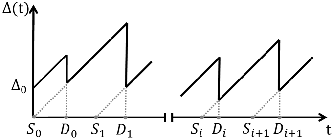
Figure 1: Evolution of the age $\Delta(t)$ over time.

Motivated by the above, this work enriches the time-lag MDP family by treating the observation delay not as a stationary stochastic variable $d$ or $D$, but as a dynamically controlled stochastic process, represented by age $\Delta(t)$ as defined in (1). We refer to this problem as age-aware remote MDP problem, where AoI serves as no longer a typical indicator but important side information for goal-oriented remote decision making. Our main result is that age-aware remote MDP, like DDMDP [5] and SDMDP [6], can also be reduced to a standard MDP problem with a constraint. We design efficient algorithms to solve this type of standard MDP with a constraint. To the best of our knowledge, this is the first work that introduces AoI into the time-lag MDP family, and the first work that explores AoI’s new role as side information to facilitate remote decision making under random delay.

II System Model and Problem Formulation

We consider a time-slotted age-aware remote MDP problem illustrated in Fig. 2(c). Let $X_{t}\in\mathcal{S}$ be the controlled source at time slot $t$. The evolution of the source is a Markov decision process, characterized by the transition probability $\Pr(X_{t+1}|X_{t},a_{t})$, where $a_{t}\in\mathcal{A}$ represents the action taken by the remote decision maker to control the source in the desired way. The sampler conducts the sampling action $a_{t}^{S}\in\{0,1\}$, with $a_{t}^{S}=1$ representing the sampling action and $a_{t}^{S}=0$ otherwise. Let $S_{i}$ be the sampling time of the $i$-th delivered packet, and $D_{i}$ be the corresponding delivery slot. Consider the random channel delay of the $i$-th packet as $Y_{i}\in\mathcal{Y}\subseteq\mathbb{N}^{+}$, which is independent of the source $X_{t}$ and is bounded $\max[{Y_{i}}]<\infty$. The sampling times $S_{0},S_{1},\cdots$ shown in Fig. 1 record the time stamp with $a_{t}^{S}=1$, given by

$$S_{i}=\max\{t\left|t\leq D_{i},a_{t}^{S}=1\right.\},$$ (2)

where the initial state of the system is $S_{0}=0$ and $\Delta(0)=\Delta_{0}$.

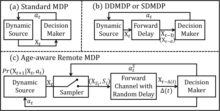
Figure 2: Comparisons among standard MDP, DDMDP, SDMDP, and age-aware remote MDP.

At the sampling time $S_{i},\forall i\in\mathbb{N}$, the state $X_{S_{i}}$ along with the corresponding time stamp $S_{i}$ are encapsulated into a packet $(X_{S_{i}},S_{i})$, which is transmitted to a remote decision maker. Upon the reception of the packet $(X_{S_{i}},S_{i})$ during $t\in[D_{i},D_{i+1})$, the observation history at the decision maker is $\{(X_{S_{j}},S_{j}):{j\leq i}\}$. By employing (1), this sequence can be equivalently represented as $\{(X_{k-\Delta(k)},\Delta(k)):{k\leq t}\}$.

Denote $\mathcal{I}_{t}=\{(X_{k-\Delta(k)},\Delta(k),a_{k-1}^{S},a_{k-1}):{k\leq t}\}$ as the observation history and action history (or simply history) available to the decision maker up to time $t$. The decision maker is tasked with determining both the sampling action and the controlled action $(a_{t}^{S},a_{t})\in\{0,1\}\times\mathcal{A}$ at each time slot $t$ by leveraging the history $\mathcal{I}_{t}$. A decision policy of the decision maker is defined as a mapping from the history to a distribution over the joint action space $\{0,1\}\times\mathcal{A}$, denoted by $\pi_{t}:\mathcal{I}_{t}\rightarrow\mathrm{Prob}(\mathcal{A}\times\{0,1\})$. Similar to [1], we assume that the sampling policy satisfies two conditions:

• $i$) No sample is taken when the channel is busy, i.e., $S_{i+1}\geq D_{i}$, or equivalently,

  $$S_{i+1}-Z_{i}=D_{i}\text{ with }Z_{i}\geq 0,i\in\mathbb{N},$$ (3)

  with $Z_{i}$ representing the sampling waiting time. From this assumption, we can also obtain that $D_{i}=S_{i}+Y_{i},\forall i\in\mathbb{N}$.

• $ii$) The inter-sample times $G_{i}=S_{i+1}-S_{i}$ is a regenerative process [38, Section 6.1]: There is a sequence $0\leq g_{1}<g_{2}<\cdots$ of almost surely finite random integers such that the post-$g_{j}$ process $\{G_{{g_{j}}+i}\}_{i\in\mathbb{N}}$ has the same distribution as the post-$g_{1}$ process $\{G_{{g_{1}}+i}\}_{i\in\mathbb{N}}$ and is independent of the pre-$g_{j}$ process $\{G_{{g_{1}}+i}\}_{i\in\{0,1,\cdots k_{j}-1\}}$. Condition $ii$) implies that, almost surely

  $$\lim\limits_{i\rightarrow\infty}S_{i}=\infty,~{}~{}~{}\lim\limits_{i\rightarrow\infty}D_{i}=\infty.$$ (4)

In addition, we assume that the controlled policy satisfies the following condition: the action $a_{t}$ is updated only upon the delivery of a sample $X_{S_{i}}$, i.e.,

$$a_{t}=A_{i},D_{i}\leq t\leq D_{i+1},i\in\mathbb{N},$$ (5)

where $A_{i}\in\mathcal{A}$ is the updated controlled action upon the delivery of packet $(X_{S_{i}},S_{i})$. We consider bounded cost function $\mathcal{C}(X_{t},a_{t})<\infty$, which represents the immediate cost incurred when action $a_{t}$ is taken in state $X_{t}$. Under the above assumptions, the objective of the system is to design the optimal policies at each time slot $\pi_{0},\pi_{1},\pi_{2}\cdots$ to minimize the long-term average cost:

$$\mathcal{P}1:\inf_{\pi_{0:\infty}}\limsup_{T\rightarrow\infty}\frac{1}{T}\mathbb{E}\left[\sum_{t=1}^{T}\mathcal{C}(X_{t},a_{t})\right].$$ (6)

Since age $\Delta(k)$ is available at the decision maker as side information to facilitate the decision-making process, we call this problem as an age-aware remote MDP problem. This problem aims at determining the distribution of joint sampling and controlled actions $(a_{t}^{S},a_{t})$ based on the history $\mathcal{I}_{t}$, such that the long-term average cost is minimized.

III Optimal Sampling and Remote Decision Making Policy Under Random Delay

III-A Sufficient Statistics of History

The policy $\pi_{t}$ is a mapping from $\mathcal{I}_{t}$ to the action provability space. One challenge to solving $\pi_{t}$ is that the history space $\mathcal{I}_{t}$ explodes exponentially as $t$ increases. This motivates us to compress and abstract information that is necessary for the optimal decision process. Specifically, we will analyze the sufficient statistics in this subsection.

Definition 1.

A sufficient statistics of $\mathcal{I}_{t}$ is a function $S_{t}(\mathcal{I}_{t})$, such that $\min_{a_{t:T}}\mathbb{E}\left[\sum_{k=t}^{T}\mathcal{C}(X_{k},a_{k})|\mathcal{I}_{t}\right]=\min_{a_{t:T}}\mathbb{E}\left[\sum_{k=t}^{T}\mathcal{C}(X_{k},a_{k})|S_{t}(\mathcal{I}_{t})\right]$ holds for any $T>t$.

The above definition implies that the decision making based on the sufficient statistics $H_{t}(\mathcal{I}_{t})$ can achieve an equivalent performance as that dependent on $\mathcal{I}_{t}$. The following lemma demonstrates an important sufficient statistics of $\mathcal{I}_{t}$.

Lemma 1.

During the interval $t\in[D_{i},D_{i+1})$, $\mathcal{G}_{i}=(X_{S_{i}},Y_{i},A_{i-1})\in\mathcal{S}\times\mathcal{Y}\times\mathcal{A}$ is a sufficient statistics of $\mathcal{I}_{t}$. Besides, determining the optimal sampling actions $a_{t}^{S}$ under condition (3) is equivalent to determining the optimal sampling time $S_{i+1}$, or the optimal waiting time $Z_{i}$.

Proof.

See Appendix A. ∎

With Lemma 1, determining the optimal policy $\pi_{t}:\mathcal{I}_{t}\rightarrow\mathrm{Prob}(\mathcal{A}\times\{0,1\})$ for $\mathcal{P}1$ becomes equivalent to solving for an alternative policy $\phi_{t}:\mathcal{S}\times\mathcal{Y}\times\mathcal{A}\rightarrow\mathrm{Prob}(\mathbb{N}\times\mathcal{A})$, which is a mapping from $\mathcal{G}_{i}$ to a distribution of $(Z_{i},A_{i})$. The problem $\mathcal{P}1$ is thus rewritten as

$$\mathcal{P}2:\inf_{\phi_{0:\infty}}\limsup_{T\rightarrow\infty}\frac{1}{T}\mathbb{E}\left[\sum_{t=1}^{T}\mathcal{C}(X_{t},a_{t})\right].$$ (7)

III-B Simplification of Problem $\mathcal{P}2$

As the inter-sampling times $G_{i}$ is a regenerative process and $\lim\limits_{i\rightarrow\infty}D_{i}=\infty$, we can rewrite the objective function in problem $\mathcal{P}2$ as

$$\limsup_{T\rightarrow\infty}\frac{1}{T}\mathbb{E}\left[\sum_{t=1}^{T}\mathcal{C}(X_{t},a_{t})\right]$$

$$=\lim_{\it{D}_{\mathrm{n}}\rightarrow\infty}\frac{\mathbb{E}\left[\sum_{t=1}^{\it{D}_{\mathrm{n}}}\mathcal{C}(X_{t},a(t))\right]}{\mathbb{E}\left[\it{D}_{\mathrm{n}}\right]}$$

$$=\lim_{\mathrm{n}\rightarrow\infty}\frac{\sum_{i=0}^{n-1}\mathbb{E}\left[\sum_{t=\it{D}_{i}}^{\it{D}_{i+1}-1}\mathcal{C}(X_{t},A_{i})\right]}{\sum_{i=0}^{n-1}\mathbb{E}\left[\it{D}_{i+1}-\it{D}_{i}\right]}$$

$$=\lim_{\mathrm{n}\rightarrow\infty}\frac{\sum_{i=0}^{n-1}\mathbb{E}\left[\sum_{t=\it{D}_{i}}^{\it{D}_{i+1}-1}\mathcal{C}(X_{t},A_{i})\right]}{\sum_{i=0}^{n-1}\mathbb{E}\left[Y_{i+1}+Z_{i}\right]}.$$ (8)

Then Problem $\mathcal{P}2$ can be rewritten as

$$\mathcal{P}3:h^{*}\triangleq\inf_{\phi_{0:\infty}}\lim_{\mathrm{n}\rightarrow\infty}\frac{\sum_{i=0}^{n-1}\mathbb{E}\left[\sum_{t=\it{D}_{i}}^{\it{D}_{i+1}-1}\mathcal{C}(X_{t},A_{i})\right]}{\sum_{i=0}^{n-1}\mathbb{E}\left[Y_{i+1}+Z_{i}\right]}.$$ (9)

To solve Problem $\mathcal{P}3$, we consider the following problem with parameter $\lambda\geq 0$:

By similarly applying Dinkelbach’s method for nonlinear fractional programming as in [39] and [21, Lemma 2], we can obtain the following lemma:

Lemma 2.

The following assertions hold:
(i). $h^{*}\gtreqless\lambda\text{ if and only if }U(\lambda)\gtreqless 0\text{. }$
(ii). When $U(\lambda)=0$, the solutions to Problem $\mathcal{P}4$ coincide with those of Problem $\mathcal{P}3$.
(iii). $U(\lambda)=0$ has a unique root, and the root is $h^{*}$.

Proof.

See Appendix B. ∎

Following Lemma 2, solving Problem $\mathcal{P}3$ can be simplified to solving Problem $\mathcal{P}4$ under $U(\lambda)=0$. Our remaining goal is to solve $\mathcal{P}4$ and search $h^{*}$ such that the optimal value of Problem $\mathcal{P}4$ is zero, i.e., $U(h^{*})=0$.

III-C Reformulate Problem $\mathcal{P}4$ as a Standard MDP

In this subsection, we formulate Problem $\mathcal{P}4$ as a standard infinite horizon MDP problem. We introduce the state space, action space, transition probability, and cost function of the MDP problem in this subsection specifically. This MDP problem with parameter $\lambda$ is denoted as $\mathscr{P}_{\mathrm{MDP}}(\lambda)$:

• State Space: the state of the equivalent MDP is the sufficient statistics $\mathcal{G}_{i}=(X_{S_{i}},Y_{i},A_{i-1})\in\mathcal{S}\times\mathcal{Y}\times\mathcal{A}$.

• Action Space: the actions space of the MDP composed by the tuple $(Z_{i},A_{i})\in\mathcal{\mathcal{Z}\times\mathcal{A}}$, where $Z_{i}$ is the sampling waiting time and $A_{i}$ is the controlled actions.

• Transition Probability: The transition probability is defined by $\Pr(\mathcal{G}_{i+1}|\mathcal{G}_{i},Z_{i},A_{i})$. We have the transition probability as (see Appendix C for the detailed proof):

  $$\Pr(\mathcal{G}_{i}=(s^{\prime},\delta^{\prime},a^{\prime})|\mathcal{G}_{i}=(s,\delta,a),Z_{i},A_{i})$$ (11)

  $$=\Pr(Y_{i+1}=\delta^{\prime})\cdot[\mathbf{P}_{a}^{\delta}\cdot\mathbf{P}_{a_{i}}^{Z_{i}}]_{s\times s^{\prime}}\cdot\mathbbm{1}\{a^{\prime}=A_{i}\},$$

• Cost Function: the cost function is typically a real-valued function over the state space and the action space. We denote the cost function as $g(\mathcal{G}_{i},Z_{i},A_{i})$, and next show that we can tailor the cost function to establish an identical standard MDP of Problem $\mathcal{P}4$.

  Lemma 3.

  If the cost function is defined by

  $$g(\mathcal{G}_{i},Z_{i},A_{i};\lambda)\triangleq q(\mathcal{G}_{i},Z_{i},A_{i})-\lambda f(Z_{i}),$$ (12)

  where

  $$f(Z_{i})=Z_{i}+\mathbb{E}\left[Y_{i+1}\right],$$ (13)

  then Problem $\mathscr{P}_{\mathrm{MDP}}(\lambda)$ is identical to Problem $\mathcal{P}4$.

  Proof.

  See Appendix D. ∎

Our remaining focus is to solve $\mathscr{P}_{\mathrm{MDP}}(\lambda)$ and seek a value $h^{*}$ such that the long-term average cost of $\mathscr{P}_{\mathrm{MDP}}(h^{*})$ is zero.

III-D Existence of Optimal Stationary Deterministic Policy

We examine the sufficient conditions required for the existence of a stationary deterministic policy within $\mathscr{P}_{\mathrm{MDP}}(\lambda)$. Our main result is described in the following theorem:

Theorem 1.

If an MDP characterized by finite state space $\mathcal{S}$, finite action space $\mathcal{A}$, and transition probability $\mathbf{P}_{a}$ is a unichain, then an optimal stationary deterministic policy exists for the MDP $\mathscr{P}_{\mathrm{MDP}}(\lambda)$.

Proof.

See Appendix E. ∎

III-E Numerical Solutions

We propose two algorithms to solve the infinite-horizon MDP and seek the parameter $h^{*}$ such that $U(h^{*})=0$.

$\bullet$ Bisec-RVI: The first one is a two-layer algorithm. The outer layer is based on the bisection-search method: the search interval $(\lambda_{\downarrow}^{(k)},\lambda_{\uparrow}^{(k)})$ is iteratively narrowed down by half until the interval can closely approximate the value $h^{*}$ such that $U(h^{*})=0$. The internal layer utilizes Relative Value Iteration (RVI) to compute the value $U(\lambda)$ by resolving the MDP $\mathscr{P}_{\mathrm{MDP}}(\lambda)$. A similar two-layer bisection-based method has been introduced in [1, 21] and [40] to achieve Age-optimal or Mean Square Error (MSE)-optimal sampling. We note the complexity of Bisec-RVI algorithm is dependent on the initialization of the search interval $(\lambda_{\downarrow},\lambda_{\uparrow})$, and thus establish a general upper and lower bound of $h^{*}$ to facilitate the search:

Lemma 4.

The lower bound of $h^{*}$ can be defined by the minimum value of the cost function, given by

$$h^{*}\geq\min_{s,a}\mathcal{C}(s,a).$$ (15)

The upper bound of $h^{*}$ can be defined by the minimum stationary cost achievable under a constant action, given by

$$h^{*}\leq\min_{a}\sum_{s\in\mathcal{S}}{\pi}_{a}(s)\cdot\mathcal{C}(s,a),$$ (16)

where ${\pi}_{a}(s)$ represents the stationary distribution of state $s$, corresponding to the transition probability matrix $\mathbf{P}_{a}$.

Proof.

See Appendix F. ∎

The Bisec-RVI Algorithm is detailed in Algorithm 1, where the RVI algorithm is a mature technique to solve an infinite-horizon MDP. We refer [41, Section 6.5.2] and [42, Section 8.5.5] for the details of RVI.

Input: Tolerence $\epsilon>0$, MDP $\mathscr{P}_{\mathrm{MDP}}(\lambda)$

1 Initialization: $\lambda_{\uparrow}=\min_{a}\sum_{s\in\mathcal{S}}{\pi}_{a}(s)\cdot\mathcal{C}(s,a)$, $\lambda_{\downarrow}=\min_{s,a}\mathcal{C}(s,a)$ ;

2 while $\lambda_{\uparrow}-\lambda_{\downarrow}\geq\epsilon$ do

3       $\lambda=(\lambda_{\uparrow}+\lambda_{\downarrow})/2$;

4       Run RVI to solve $\mathscr{P}_{\mathrm{MDP}}(\lambda)$ and calculate $U(\lambda)$;

5       if $U(\lambda)>0$ then

6             $\lambda_{\downarrow}=\lambda$;

7            

8      else

9            $\lambda_{\uparrow}=\lambda$;

10      

Output: $h^{*}=\lambda$

Algorithm 1 Bisec-RVI algorithm

$\bullet$ Fixed-Point-Based Iteration (FPBI): The Bisec-RVI algorithm requires repeatedly executing the RVI algorithm, which is computation-intensive. This motivates us to propose a one-layer algorithm, which differs significantly from the two-layer Bisec-RVI approach. Unlike the latter, which relies on an outer-layer search to find a value $h^{*}$ such that $U(h^{*})=0$, the one-layer FPBI algorithm treats $U(h^{*})=0$ as a constraint within the Markov Decision Process $\mathscr{P}_{\mathrm{MDP}}(h^{*})$. Our main contribution is the following equivalent equations.

Theorem 2.

Solving Problem $\mathscr{P}_{\mathrm{MDP}}(h^{*})$ with $U(h^{*})=0$ is equivalent to solving the following nonlinear equations:

$$\left\{\begin{aligned} &W^{*}(\gamma)=\min_{A_{i},Z_{i}}\big{\{}g(\gamma,A_{i},Z_{i};h^{*})+\mathbb{E}[W^{*}\left(\gamma^{\prime}\right)|\gamma,Z_{i},A_{i}]\big{\}}\\ &\text{for }\gamma\in\mathcal{S}\times\mathcal{Y}\times\mathcal{A},\\ &h^{*}=\min_{A_{i},Z_{i}}\left\{\frac{q\left(\gamma^{\mathrm{ref}},A_{i},Z_{i}\right)+\mathbb{E}[W^{*}\left(\gamma^{\prime}\right)|\gamma^{\mathrm{ref}},A_{i},Z_{i}]}{f\left(Z_{i}\right)}\right\},\\ \end{aligned}\right.$$ (17)

where $\gamma^{\mathrm{ref}}\in\mathcal{S}\times\mathcal{Y}\times\mathcal{A}$ can be arbitrarily chosen.

Proof.

See Appendix G. ∎

In (17), there are $|\mathcal{S}|\times|\mathcal{Y}|\times|\mathcal{A}|+1$ variables, i.e., $h^{*}$ and $W^{*}(\gamma),\gamma\in\mathcal{S}\times\mathcal{Y}\times\mathcal{A}$, matched by an equal number of equations. We next show (17) is a fixed-point equation. Let $\mathbf{W}^{*}$ denote the vector consisting of $W^{*}(\gamma)$ for all $\gamma\in\mathcal{S}\times\mathcal{Y}\times\mathcal{A}$, (17) can be succinctly represented as follows:

$$\left\{\begin{aligned} &\mathbf{W}^{*}=T(\mathbf{W}^{*},h^{*})\\ &h^{*}=H(\mathbf{W}^{*}).\end{aligned}\right.$$ (18)

Substituting the second equation $h^{*}=H(\mathbf{W}^{*})$ into the first equation of (18) yields $\mathbf{W}^{*}=T(\mathbf{W}^{*},H(\mathbf{W}^{*}))$. Define $Q(\mathbf{W})\triangleq T(\mathbf{W},H(\mathbf{W}))$ for simplification. Consequently, as implied by (18), we have the fixed-point equation:

$$\mathbf{W}^{*}=Q(\mathbf{W}^{*}),$$ (19)

which can be solved by fixed-point iteration in Algorithm 2.

Figure 3: Average age and average cost vs. $p$ with i.i.d random delay $Y_{i}$, where $\Pr(Y_{i}=1)=p$ and $\Pr(Y_{i}=10)=1-p$.

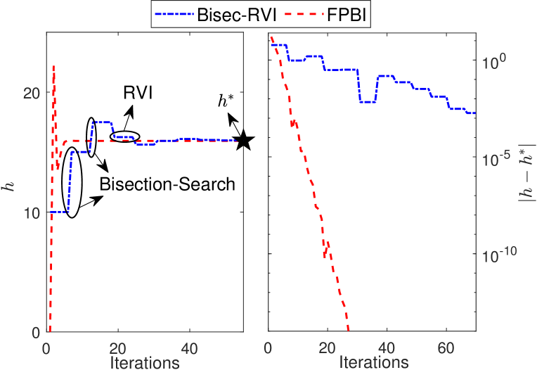
Figure 4: Bisec-RVI vs. FPBI, where $p=0.3$.

Input: MDP $\mathscr{P}_{\mathrm{MDP}}(\lambda)$, Tolerence $\epsilon$;

1 Initialization: $\mathbf{W}^{*}_{(0)}=\mathbf{0}$, $\mathbf{W}^{*}_{(-1)}=\infty$, $k=0$ ;

2 Choose $\gamma^{ref}$ arbitrarily;

3 while $||\tilde{V}_{\pi_{A}}^{k}(\mathbf{w})-\tilde{V}_{\pi_{A}}^{k-1}(\mathbf{w})||\geq\epsilon$ do

4       $k=k+1$;

5       $h^{*}_{(k)}=H(\mathbf{W}^{*}_{(k-1)})$;

6       $\mathbf{W}^{*}_{(k)}=T(\mathbf{W}^{*}_{(k-1)},h^{*}_{(k)})$;

      // See (17) and (18) for $T(\cdot)$ and $H(\cdot)$.

7      

Output: $h^{*}=h^{*}_{(k)}$

Algorithm 2 FPBI for Solving (17)

IV Simulation Results

In this paper, the policy that minimizes the long-term average cost in Problem $\mathcal{P}1$ is referred to as “optimal policy”. We compare it with the following two benchmarks:

• Zero wait: An update is transmitted once the previous update is delivered, i.e., $Z_{i}=0$ for $\forall i$. This policy achieves the minimum delay and maximum throughput. The controlled action $a_{i}$ is age-aware and is obtained by substituting $Z_{i}=0$ into the RHS of (17) and similarly implementing the fixed-point iteration, implying age-aware optimal control under zero-wait sampling.

• AoI-optimal: The AoI-optimal policy determines $Z_{i}$ by [1, Theorem 4], which is a threshold-based policy $Z_{i}=\max(0,\beta-Y_{i})$, where $\beta$ is numerically solved by [1, Algorithm 2]. The controlled action $a_{i}$ is age-aware and is obtained by fixing the AoI-optimal sampling in (17) and similarly implementing the fixed-point iteration, implying age-aware optimal control under AoI-optimal sampling.

As a case study, we consider the parameters detailed in Appendix H for the simulation setup.

Fig. 3 compares the benchmarks with “optimal policy” in terms of average age and cost. The left panel demonstrates that the AoI-optimal policy consistently achieves the lowest age. However, the right panel reveals a counterintuitive result: the AoI-optimal policy does not necessarily lead to the best decision-making performance. This suggests that the value-of-information transcends mere age freshness; it is also shaped by the specific goal of the receiver and the semantic content of the information [43, 44, 45, 46]. The “optimal policy” consistently yields the lowest average cost and the performance gap between the “optimal policy” and others widens as the average delay, $\mathbb{E}[Y_{i}]=10-9p$, increases.

Fig. 4 compares FPBI with Bisec-RVI, employing the latter as a benchmark. This benchmark is inspired by the two-layer solution frameworks by [1, 21] and [40]. The left panel records the trajectories of $h$ across algorithms iterations, illustrating that both Bisec-RVI and FPBI converge to the optimal $h^{*}$. For Bisec-RVI, updates to $h$ are deponent on the outer-layer bisection search, which occur only upon the convergence of the inter-layer RVI. In contrast, our developed one-layer FPBI innovatively eliminates the need for the outer-layer bisection search by fixing $U(h^{*})=0$ and directly establishing fixed point equations for $\mathscr{P}_{\mathrm{MDP}}(h^{*})$ under this condition. The right panel records the distances to $h^{*}$ across algorithms iterations, which clearly demonstrated that FPBI algorithm achieves faster convergence compared Bisec-RVI.

V Conclusion

In this paper, we have proposed a new remote MDP problem in the time-lag MDP framework, termed age-aware remote MDP. Specifically, AoI, typically an optimization indicator to ensure information freshness, has been introduced into the remote MDP problem as a specific category of controlled random processing delay and as important side information to enhance remote decision-making. The main result of this work is that the age-aware remote MDP can be reformulated into a standard, delay-free MDP. Under such an equivalent problem, we have established sufficient conditions for the existence of an optimal stationary deterministic policy. Additionally, we have developed a low-complexity one-layer algorithm to effectively solve this remote MDP problem. We revealed that the age-optimal policy, which ensures the freshest information, does not necessarily achieve the best remote decision making. In contrast, we can design goal-oriented sampling that directly optimize remote decision making.

Appendix A Proof of Lemma 1

A-A Proof of Sufficient Statistics

We begin with rewriting the conditional expectation:

$$\max_{a_{t:T}}\mathbb{E}\left[\sum_{k=t}^{T}\mathcal{C}(X_{k},a_{k})|\mathcal{I}_{t}\right]$$ (20)

$$=\max_{a_{t:T}}\sum_{k=t}^{T}\mathcal{C}(s^{\prime},a_{k})\cdot\Pr(X_{k}=s^{\prime}\mid\mathcal{I}_{t}).$$

Because $X_{k}$ is a Markov decision process, the conditional probability $\Pr(X_{k}=s^{\prime}\mid\mathcal{I}_{t})$, where $\mathcal{I}_{t}$ is defined as $\mathcal{I}_{t}\triangleq\{(X_{k-\Delta(k)},\Delta(k),a_{k-1}^{S},a_{k-1}):{k\leq t}\}$, is only dependent on the most recently available information $X_{t-\Delta(t)}$, the age of the most recently available information $\Delta(t)$, and the actions taken from time slot $t-\Delta(t)$ to time slot $t$, $a_{t-\Delta(t):t}$. Thus, we can rewrite the conditional probability in (20) as:

$$\Pr(X_{k}=s^{\prime}\mid\mathcal{I}_{t})$$ (21)

$$=\Pr\left(X_{k}=s^{\prime}\mid X_{t-\Delta(t)},\Delta(t),a_{t-\Delta(t):t-1}\right).$$

For $t$ within the interval $[D_{i},D_{i+1})$, equation (1) implies that $t-\Delta(t)=S_{i}$. This allows us to deduce the right-hand side (RHS) of (21) as

$$\Pr\left(X_{k}=s^{\prime}\mid X_{S_{i}},t-S_{i},a_{S_{i}:t-1}\right)$$ (22)

$$=\Pr\left(X_{k}=s^{\prime}\mid X_{S_{i}},t-S_{i},a_{S_{i}:D_{i}-1},a_{D_{i}:t-1}\right)$$

$$=\Pr\left(X_{k}=s^{\prime}\mid X_{S_{i}},t-D_{i}+Y_{i},A_{i-1},a_{D_{i}:t-1}\right).$$

Because $t$ and $D_{i}$ are both known to the decision maker during the interval $t\in[D_{i},D_{i+1})$, i.e., $t$ and $D_{i}$ are deterministic, the conditional probability can be rewritten as

$$\Pr\left(X_{k}=s^{\prime}\mid X_{S_{i}},Y_{i},A_{i-1},a_{D_{i}:t-1}\right).$$ (23)

Substituting (23) into (20) yields

Because $a_{t}$ is a constant during the interval $[D_{i},D_{i+1})$, we have that

$$a_{D_{i}:t-1}=a_{t},\text{for }t\in[D_{i},D_{i+1}).$$ (25)

We can thus rewrite the RHS of (24) as

$$\max_{a_{t:T}}\sum_{k=t}^{T}\mathcal{C}(s^{\prime},a_{k})\cdot\Pr\left(X_{k}=s^{\prime}\mid X_{S_{i}},Y_{i},A_{i-1},a_{t}\right)$$ (26)

$$=\max_{a_{t:T}}\mathbb{E}_{a_{t:T}}\left[\sum_{k=t}^{T}\mathcal{C}(X(k),a_{k})\mid X_{S_{i}},Y_{i},A_{i-1}\right].$$

From Definition 1 and we know that $X_{S_{i}},Y_{i},A_{i-1}$ is a sufficient statistics of $\mathcal{I}_{t}$ for $t\in[D_{i},D_{i+1})$.

A-B Determining $a_{t}^{S}$ is equivalent to Determining $Z_{i}$

By combing (2) and (3), we have that the sequence $\{a_{t}^{S}\}_{t\in[D_{i},D_{i+1})}$ constitutes a one-to-one mapping either to the sampling time $S_{i+1}$ or to the waiting time $Z_{i}$. Therefore, determining the sequence $\{a_{t}^{S}\}_{t\in[D_{i},D_{i+1})}$ is equivalent to determine $S_{i+1}$ or $Z_{i}$.

Appendix B Proof of Lemma 2

B-A Proof of Part (i)

B-A1 $h^{*}\leq\lambda\iff U(\lambda)\leq 0$

If $h^{*}\leq\lambda$, there exists a policy $\pi=(Z_{0},A_{0},Z_{1},A_{1},\cdots)$ such that

$$\lim_{\mathrm{n}\rightarrow\infty}\frac{\sum_{i=0}^{n-1}\mathbb{E}_{\pi}\left[\sum_{t=\it{D}_{i}}^{\it{D}_{i+1}-1}\mathcal{C}(X_{t},A_{i})\right]}{\sum_{i=0}^{n-1}\mathbb{E}_{\pi}\left[Y_{i+1}+Z_{i}\right]}\leq\lambda,$$ (27)

which is equivalent to

Since $Y_{i}>0$ and $0\leq Z_{i}<\infty$, we have that $\lim_{\mathrm{n}\rightarrow\infty}\frac{1}{n}\sum_{i=0}^{n-1}\mathbb{E}\left[Y_{i+1}+Z_{i}\right]$ always exists, satisfying

$$0<\lim_{\mathrm{n}\rightarrow\infty}\frac{1}{n}\sum_{i=0}^{n-1}\mathbb{E}\left[Y_{i+1}+Z_{i}\right]<\infty$$ (29)

for any policies. Thus, we have that the numerator of (28) satisfies

$$\lim_{\mathrm{n}\rightarrow\infty}\frac{1}{n}\sum_{i=0}^{n-1}\mathbb{E}_{\pi}\left[\sum_{t=\it{D}_{i}}^{\it{D}_{i+1}-1}\mathcal{C}(X_{t},A_{i})\right]-\lambda\mathbb{E}_{\pi}[Z_{i}+Y_{i+1}]\leq 0.$$ (30)

This implies that the infimum of the left-hand side of (30) is also at most $0$, i.e, $U(\lambda)\leq 0$.

On the contrary, when $U(\lambda)\leq 0$, we can know that there exists a policy $\pi=(Z_{0},A_{0},Z_{1},A_{1},\cdots)$ that satisfies (30). As (29) always holds, we can easily obtain that (27) holds. Note that $h^{*}$ is the infimum of the left hand side of (27), we have

$$h^{*}\leq\lim_{\mathrm{n}\rightarrow\infty}\frac{\sum_{i=0}^{n-1}\mathbb{E}_{\pi}\left[\sum_{t=\it{D}_{i}}^{\it{D}_{i+1}-1}\mathcal{C}(X_{t},a_{i})\right]}{\sum_{i=0}^{n-1}\mathbb{E}_{\pi}\left[Y_{i+1}+Z_{i}\right]}\leq\lambda.$$ (31)

B-A2 $h^{*}>\lambda\iff U(\lambda)>0$

If $h^{*}>\lambda$, we have that for any policy $(Z_{0},A_{0},Z_{1},A_{1},\cdots)$, the following inequality always holds

$$\lim_{\mathrm{n}\rightarrow\infty}\frac{\sum_{i=0}^{n-1}\mathbb{E}\left[\sum_{t=\it{D}_{i}}^{\it{D}_{i+1}-1}\mathcal{C}(X_{t},A_{i})\right]}{\sum_{i=0}^{n-1}\mathbb{E}\left[Y_{i+1}+Z_{i}\right]}>\lambda.$$ (32)

Since (29) holds, we have that for any policy $(Z_{0},A_{0},Z_{1},A_{1},\cdots)$,

$$\lim_{\mathrm{n}\rightarrow\infty}\frac{1}{n}\sum_{i=0}^{n-1}\mathbb{E}\left[\sum_{t=\it{D}_{i}}^{\it{D}_{i+1}-1}\mathcal{C}(X_{t},A_{i})\right]-\lambda\mathbb{E}[Z_{i}+Y_{i+1}]>0.$$ (33)

Since (33) holds for any policies, it follows that the infimum value of the left-hand side (LHS) of (33) is also greater than $0$, implying that $h^{*}>\lambda$.

When $U(\lambda)>0$, it is established that condition (33) is satisfied for any policy sequence $(Z_{0},A_{0},Z_{1},A_{1},\cdots)$. Given that (29) always holds, it follows directly that (32) holds for any policies, implying that the infimum of the LHS of (32) is also greater than $\lambda$, i.e., $h^{*}>\lambda$.

B-B Proof of Part (ii)

Through the proof of Part (ii), we know that $U(\lambda)=0$ is equivalent to $\lambda=h^{*}$. If $U(\lambda)=0$, we know that there exists an optimal policy $\pi^{*}=(Z_{0},A_{0},Z_{1},A_{1},\cdots)$ for Problem $\mathcal{P}4$, satisfying that

$$\lim_{\mathrm{n}\rightarrow\infty}\frac{1}{n}\sum_{i=0}^{n-1}\mathbb{E}\left[\sum_{t=\it{D}_{i}}^{\it{D}_{i+1}-1}\mathcal{C}(X_{t},A_{i})\right]-\lambda(Z_{i}+Y_{i+1})=0,$$ (34)

which implies that for the policy $\pi^{*}$,

$$\lim_{\mathrm{n}\rightarrow\infty}\frac{\sum_{i=0}^{n-1}\mathbb{E}\left[\sum_{t=\it{D}_{i}}^{\it{D}_{i+1}-1}\mathcal{C}(X_{t},A_{i})\right]}{\sum_{i=0}^{n-1}\mathbb{E}\left[Y_{i+1}+Z_{i}\right]}=\lambda.$$ (35)

Note that $h^{*}=\lambda$, we have that for the policy $\pi^{*}$,

$$h^{*}=\lim_{\mathrm{n}\rightarrow\infty}\frac{\sum_{i=0}^{n-1}\mathbb{E}\left[\sum_{t=\it{D}_{i}}^{\it{D}_{i+1}-1}\mathcal{C}(X_{t},A_{i})\right]}{\sum_{i=0}^{n-1}\mathbb{E}\left[Y_{i+1}+Z_{i}\right]},$$ (36)

which infers that policy $\pi^{*}$ is also the optimal policy of Problem $\mathcal{P}3$.

B-C Proof of Part (iii)

From Part (i), we know that proving Part (iii) is equivalent to prove that $U(\lambda)$ is monotonically non-increasing in terms of $\lambda$, i.e., for any $\Delta\lambda>0$, $U(\lambda+\Delta\lambda)\leq U(\lambda)$. This is verified by the following inequalities:

Thus, we have that $\lambda=h^{*}$ is the unique root of $U(\lambda)=0$.

Appendix C Transition Probability of $\mathscr{P}_{\mathrm{MDP}}(\lambda)$

We first calculate $\Pr\left(X_{S_{i+1}}|\mathcal{G}_{i},Z_{i},A_{i}\right)$ $\Pr\left(Y_{{i+1}}|\mathcal{G}_{i},Z_{i},A_{i}\right)$, $\Pr\left(A_{{i+1}}|\mathcal{G}_{i},Z_{i},A_{i}\right)$, respectively here.

C-A $\Pr\left(X_{S_{i+1}}|\mathcal{G}_{i},Z_{i},A_{i}\right)$

From time $S_{i}$ to $S_{i+1}$, the dynamics of the source $X_{t}$ can to divided into two Markov Sources

• During the interval $S_{i}\leq t\leq D_{i}$, the action remains constant $A_{i-1}=a$. Throughout this period, the system’s dynamics adhere to a Markov chain, defined by the transition probability matrix $\mathbf{P}_{A_{i-1}}$. The transitions within this interval are quantified as $D_{i}-S_{i}=Y_{i}=\delta$. Thus the transition probability can be expressed by a $\delta$-step transition probability matrix, denoted as $\mathbf{P}_{a}^{\delta}$.

• In the subsequent time slot where $D_{i}\leq t\leq S_{i+1}$, the action is consistently $A_{i}$. During this phase, the system continues as another Markov chain with transition probability matrix $\mathbf{P}_{A_{i}}$. The number of transitions occurring in this interval is $S_{i+1}-D_{i}=Z_{i}$, which leads to a $Z_{i}$-step transition probability matrix $\mathbf{P}_{A_{i}}^{Z_{i}}$.

Thus, the transition probability from $t=S_{i}$ to $t=S_{i+1}$ is the product of the $\delta$-step transition probability matrix $\mathbf{P}_{a}^{\delta}$ and the $Z_{i}$-step transition probability matrix $\mathbf{P}_{A_{i}}^{Z_{i}}$. This yields the transition probability as:

$$\Pr\left(X_{S_{i+1}}=s^{\prime}|\mathcal{G}_{i}=(s,\delta,a),Z_{i},A_{i}\right)=[\mathbf{P}_{a}^{\delta}\cdot\mathbf{P}_{A_{i}}^{Z_{i}}]_{s\times s^{\prime}}.$$ (38)

C-B $\Pr(Y_{i+1}|\mathcal{G}_{i},Z_{i},A_{i})$

Note that $Y_{i}$ is i.i.d random variable, $Y_{i+1}$ is independent of $\mathcal{G}_{i}$, $Z_{i}$, and $A_{i}$. Thus, the following transition probability is almost sure

$$\Pr\left(Y_{i+1}=\delta^{\prime}|\mathcal{G}_{i}=(s,\delta,a),Z_{i},A_{i}\right)=\Pr(Y_{i+1}=\delta^{\prime}).$$ (39)

C-C $\Pr(A_{i}|\mathcal{G}_{i},Z_{i},A_{i})$

The state $A_{i}$ is actually a record of the action taken. Thus, we have the following transition probability:

$$\Pr\left(A_{i}=a^{\prime}|\mathcal{G}_{i}=(s,\delta,a),Z_{i},A_{i}\right)=\mathbbm{1}\{a^{\prime}=A_{i}\}.$$ (40)

At last, by leveraging the conditional independence among $X_{S_{i+1}}$, $Y_{i+1}$, and $A_{i}$, $\Pr(\mathcal{G}_{i+1}|\mathcal{G}_{i},Z_{i},A_{i})$ can be decomposed into the product of $\Pr(X_{S_{i+1}}|\mathcal{G}_{i},Z_{i},A_{i})$, $\Pr(Y_{i+1}|\mathcal{G}_{i},Z_{i},A_{i})$, and $\Pr(A_{i}|\mathcal{G}_{i},Z_{i},A_{i})$, and we will have the transition probability given in (11).

Appendix D Proof of Lemma 3

If the cost function is defined as in (12), the objective of the MDP $\mathscr{P}_{\mathrm{MDP}}(\lambda)$ is given as

$$\inf_{\phi_{0:\infty}}\limsup_{T\rightarrow\infty}\frac{1}{T}\mathbb{E}\left[\sum_{t=1}^{T}g(\mathcal{G}_{i},A_{i},Z_{i};\lambda)\right]$$ (41)

$$=\inf_{\phi_{0:\infty}}\limsup_{T\rightarrow\infty}\frac{1}{T}\mathbb{E}\left[\sum_{t=1}^{T}q(\mathcal{G}_{i},A_{i},Z_{i})-\lambda\mathbb{E}[Z_{i}+Y_{i+1}]\right].$$

Comparing (41) with Problem $\mathcal{P}4$, our remaining focus is to prove that $\mathbb{E}\left[\sum_{t=\it{D}_{i}}^{\it{D}_{i+1}-1}\mathcal{C}\left(X_{t},A_{i}\right)\right]=\mathbb{E}[q(\mathcal{G}_{i},A_{i},Z_{i})]$.

$\mathbb{E}\left[\sum_{t=\it{D}_{i}}^{\it{D}_{i+1}-1}\mathcal{C}\left(X_{t},A_{i}\right)\right]$ can be decomposed as:

where the conditional expectation can be calculated by

Up to this point, our remaining focus is to calculate the conditional probability $\Pr(X_{t}=s^{\prime}\mid X_{S_{i}},Y_{i},A_{i-1})$ for $t\in[D_{i},D_{i+1}-1)$. Similar our the results about $\Pr(X_{S_{i+1}}\mid\mathcal{G}_{i},Z_{i},A_{i})$ in Appendix C-A, we also analyze the conditional probability through two steps:

• During the interval $S_{i}\leq t\leq D_{i}$, the action is $A_{i-1}$. Throughout this period, the system’s source is a Markov chain, defined by the transition probability matrix $\mathbf{P}_{a}$. The transitions within this interval are $D_{i}-S_{i}=Y_{i}$. Thus the transition probability can be expressed by a $\delta$-step transition probability matrix, denoted as $\mathbf{P}_{A_{i}-1}^{Y_{i}}$.

• In the subsequent time slot where $D_{i}\leq t\leq D_{i+1}-1$, the action $A_{i}$. During this period, the system is another Markov chain with transition probability matrix $\mathbf{P}_{A_{i}}$. The number of transitions in this interval is $t-D_{i}$, which leads to a $(t-D_{i})$-step transition probability matrix $\mathbf{P}_{A_{i}}^{t-D_{i}}$.

Thus, the transition probability from time slot $X_{S_{i}}$ to $X_{t}$, where $D_{i}\leq t\leq D_{i+1}$ is exactly the product of the $Y_{i}$-step transition probability matrix $\mathbf{P}_{A_{i-1}}^{Y_{i}}$ and the ($t-D_{i}$)-step transition probability matrix $\mathbf{P}_{A_{i}}^{t-D_{i}}$, given as:

$$\Pr(X_{t}=s^{\prime}\mid X_{S_{i}},Y_{i},A_{i-1})=\left[\mathbf{P}_{A_{i-1}}^{Y_{i}}\cdot\mathbf{P}_{A_{i}}^{t-D_{i}}\right]_{X_{S_{i}}\times s^{\prime}}.$$ (44)

By substituting (44) into (43), applying the variable substitution as $t:=t-D_{i}$, and interchanging the summation terms, we have

Then, note that the RHS of (45) is exactly the definition of $q(\mathcal{G}_{i},A_{i},Z_{i})$ as in (14), we complete the proof that $\mathbb{E}\left[\sum_{t=\it{D}_{i}}^{\it{D}_{i+1}-1}\mathcal{C}\left(X_{t},A_{i}\right)\right]=\mathbb{E}[q(\mathcal{G}_{i},A_{i},Z_{i})]$. Thus the objective of the MDP $\mathscr{P}_{\mathrm{MDP}}(\lambda)$ is equivalent to Problem $\mathcal{P}4$.

Appendix E Proof of Theorem 1

E-A Existence of Optimal Stationary Policy

According to [47, Proposition 6.2.3], optimal stationary policies exist under conditions where the cost function remains bounded, and both the state and action spaces are finite.

In our context, both the state space and the action space are finite space naturally. Our remaining focus is to verify that $g(\mathcal{G}_{i},Z_{i},A_{i};\lambda)$ is bounded. Given that $h^{*}$ (as shown in Lemma 4), $\lambda$, which needs to $\lambda$ to approach $h^{*}$, is also bounded. Because $\lambda$ is bounded, the step cost function of the MDP $\mathscr{P}_{\mathrm{MDP}}(\lambda)$, given by $g(\mathcal{G}_{i},Z_{i},A_{i};\lambda)$ in (12), is also bounded. This leads to the existence of an optimal stationary policy.

E-B Existence of Optimal Deterministic Policy

The sufficient condition of existence of an optimal deterministic policy is that the MDP is a unichain [42, Theorem 8.4.5]. Our result is that if an MDP characterized by finite state space $\mathcal{S}$, finite action space $\mathcal{A}$, and transition probability $\mathbf{P}_{a}$ is a unichain, then its corresponding remote-MDP transformation $\mathscr{P}_{\mathrm{MDP}}(\lambda)$ is also a unichain, i.e., the introduction of the observation delay $\Delta(t)$ does not change the unichain property of the MDP.

The condition that an MDP characterized by finite state space $\mathcal{S}$, finite action space $\mathcal{A}$, and transition probability $\mathbf{P}_{a}$ is a unichain implies that the transition probability $\mathbf{P}_{a}$, for any given $a\in\mathcal{A}$, is a unichain transition probability. We call a transition probability $\mathbf{P}_{a}$ is a unichain if there is a single recurrent class plus a possibly empty set of transients states [42, Section 8.3.1]. We have the following lemma:

Lemma 5.

The following statements are true:
i) If $\mathbf{P}_{a}$ is a unichain, then $\mathbf{P}_{a}^{n}$, where $n\in\mathbb{N}^{+}$ is also a unichain;
ii) If $\mathbf{P}_{a}$ and $\mathbf{P}_{b}$ are both unichains, then $\mathbf{P}_{a}\cdot\mathbf{P}_{b}$ is a unichain.

Proof.

Proof of Part i):
We first prove that if $s$ is a transient state for Markov chain $\mathbf{P}_{a}$, then it is also a transient state for $n$-step Markov chain $\mathbf{P}_{a}^{n}$. This is verified by the definition of a transient state:

$$p_{ss}^{n}\equiv 0,\text{ for any }n\in\mathbb{N}^{+}.$$ (46)

Next, we prove that if $\mathcal{X}$ is a recurrent class for Markov chain $\mathbf{P}_{a}$, then it is also a recurrent class for $n$-step Markov chain $\mathbf{P}_{a}^{n}$. For $i,j\in\mathcal{X}$, the $m$-step transition probability from state $i$ to $j$ can be calculated by:

$$p_{ij}^{m}=\sum_{k\in\mathcal{S}}\sum_{r=1}^{m-1}p_{ik}^{r}\cdot p_{kj}^{m-r}.$$ (47)

If $k$ is a transient state, then $p_{ik}^{r}\equiv 0$, thus (47) can be reduced to

$$p_{ij}^{m} =\sum_{k\in\mathcal{X}}\sum_{r=1}^{m-1}p_{ik}^{r}\cdot p_{kj}^{m-r}$$ (48)

$$\geq\sum_{r=1}^{m-1}p_{ii}^{r}\cdot p_{ij}^{m-r}.$$

Since $i,j\in\mathcal{X}$, we have that there exists positive integers $N_{ii},N_{ij}\in\mathbb{N}^{+}$ such that $p_{ii}^{N_{ii}}>0$ and $p_{ij}^{N_{ij}}>0$. Thus we can choose $m=N_{ii}+N_{ij}$ to establish

$$p_{ij}^{N_{ii}+N_{ij}}\geq\sum_{r=1}^{m-1}p_{ii}^{r}\cdot p_{ij}^{m-r}\geq p_{ii}^{N_{ii}}\cdot p_{ij}^{N_{ij}}>0.$$ (49)

From (49) we can deduce by mathematical induction to ensure that

$$p_{ij}^{N_{ij}+kN_{ii}}>0,\text{ for any $k\in\mathbb{N}^{+}$}.$$ (50)

Thus, for any $i,j\in\mathcal{X}$ and Markov chain $\mathbf{P}_{a}^{n}$ with any $n$, we can choose $nt=N_{ij}+kN_{ii}$ to hold that

$$\lim_{t\rightarrow\infty}p_{ij}^{nt}=\lim_{k\rightarrow\infty}p_{ij}^{N_{ij}+kN_{ii}}>0,$$ (51)

which implies that $i$ and $j$ are also commutative in the Markov chain $\mathbf{P}_{a}^{n}$.
Proof of Part ii):
To prove this, we first denote the recurrent class of $\mathbf{P}_{a}$ and $\mathbf{P}_{b}$ as $\mathcal{X}(a)$ and $\mathcal{X}(b)$, respectively. We also use $p_{ij}^{n}(a)$ and $p_{ij}^{b}$ to represent the transition probability from state $i$ to state $j$ after $n$ transition of chain $\mathbf{P}_{a}$ and chain $\mathbf{P}_{b}$, and $p_{ij}^{n}(ab)$ to denote the the corresponding transition probability of the chain $\mathbf{P}_{a}\cdot\mathbf{P}_{b}$. We prove Part ii) in the following cases:

• $\mathcal{X}(a)=\mathcal{X}(b)$: In such a case, for any $i,j\in\mathcal{X}(a)$, we have that

  $$\lim_{n\rightarrow\infty}p_{ii}^{n}(a)>0,\lim_{n\rightarrow\infty}p_{ij}^{n}(b)>0.$$ (52)

  Because

  $$\lim_{n\rightarrow\infty}p_{ij}^{n}(ab) =\lim_{n\rightarrow\infty}\sum_{k\in\mathcal{S}}p_{ik}^{n}(a)\cdot p_{kj}^{n}(b)$$ (53)

  $$\geq\lim_{n\rightarrow\infty}\sum_{k\in\mathcal{X}(a)}p_{ik}^{n}(a)\cdot p_{kj}^{n}(b)$$

  $$\geq\lim_{n\rightarrow\infty}p_{ii}^{n}(a)\cdot p_{ij}^{n}(b)>0,$$

  we have that $i$ and $j$ are also communicative for the chain $\mathbf{P}_{a}\cdot\mathbf{P}_{b}$. Thus, $\mathcal{X}(a)$ is a recurrent class of the chain $\mathbf{P}_{a}\cdot\mathbf{P}_{b}$. We next show that if $i\in\mathcal{S}-\mathcal{X}(a)=\mathcal{S}-\mathcal{X}(b)$ is a transient state for the chains $\mathbf{P}_{a}$ and chain $\mathbf{P}_{b}$, then $i$ is also a transient state for the chain $\mathbf{P}_{a}\cdot\mathbf{P}_{b}$, this is verified by

  $$p_{ii}^{n}(ab)=\sum_{k\in\mathcal{S}}p_{ik}^{n}(a)\cdot p_{ki}^{n}(b).$$ (54)

  Because $i$ is a transient state of the chain $\mathbf{P}_{b}$, we have that $p_{ki}^{n}(b)=0$, and thus we can deduce from (54) that $p_{ii}^{n}(ab)=0$. This implies that $i$ is also a transient state of the chain $\mathbf{P}_{a}\cdot\mathbf{P}_{b}$. Thus, in case where $\mathcal{X}(a)=\mathcal{X}(b)$, the recurrent class and the transient state of the chain $\mathbf{P}_{a}\cdot\mathbf{P}_{b}$ remains the same as that of $\mathbf{P}_{a}$ and $\mathbf{P}_{b}$. This implies that the chain $\mathbf{P}_{a}\cdot\mathbf{P}_{b}$ is also a unichain.

• $\mathcal{X}(a)\neq\mathcal{X}(b)$: In this case, we will prove that for the new chain $\mathbf{P}_{a}\cdot\mathbf{P}_{b}$, the unique recurrent class is $\mathcal{X}(a)\cup\mathcal{X}(b)$, and the other states from $\mathcal{S}-\mathcal{X}(a)\cup\mathcal{X}(b)$ are all transient states. There are four cases to describe $i,j\in\mathcal{X}(a)\cup\mathcal{X}(b)$:
  Case 1: $i\in\mathcal{X}(a)$ and $j\in\mathcal{X}(b)$. Similar to (53), we rewrite $p_{ij}^{n}(ab)$ as

  $$\lim_{n\rightarrow\infty}p_{ij}^{n}(ab) =\lim_{n\rightarrow\infty}\sum_{k\in\mathcal{S}}p_{ik}^{n}(a)\cdot p_{kj}^{n}(b)$$ (55)

  $$\geq\lim_{n\rightarrow\infty}\sum_{k\in\mathcal{X}(a)\cap\mathcal{X}(b)}p_{ik}^{n}(a)\cdot p_{kj}^{n}(b).$$

  Because $k\in\mathcal{X}(a)\cap\mathcal{X}(b)$, we have

  $$\lim_{n\rightarrow\infty}p_{ik}^{n}(a)>0,\lim_{n\rightarrow\infty}p_{kj}^{n}(b)>0.$$ (56)

  Substituting (56) into (55) yields $\lim_{n\rightarrow\infty}p_{ij}^{n}(ab)>0$.
  Case 2. $i\in\mathcal{X}(a)$ and $j\in\mathcal{X}(a)$. From (52) and (53) we have that $\lim_{n\rightarrow\infty}p_{ij}^{n}(ab)>0$.
  Case 3. $i\in\mathcal{X}(b)$ and $j\in\mathcal{X}(a)$. This is a symmetry consequence of Case 1 and thus we have that $\lim_{n\rightarrow\infty}p_{ij}^{n}(ab)>0$.
  Case 4. $i\in\mathcal{X}(b)$ and $j\in\mathcal{X}(b)$. This is a symmetry consequence of Case 2 and thus we have that $\lim_{n\rightarrow\infty}p_{ij}^{n}(ab)>0$.

  Thus, we can conclude that for any $i,j\in\mathcal{X}(a)\cup\mathcal{X}(b)$, $i$ and $j$ are communicative with each other for the chain $\mathbf{P}_{a}\cdot\mathbf{P}_{b}$, and thus $\mathcal{X}(a)\cup\mathcal{X}(b)$ is a recurrent class of the chain $\mathbf{P}_{a}\cdot\mathbf{P}_{b}$. We next prove that states from $\mathcal{S}-\mathcal{X}(a)\cup\mathcal{X}(b)$ are all transient states for the chain $\mathbf{P}_{a}\cdot\mathbf{P}_{b}$. Suppose $i\in\mathcal{S}-\mathcal{X}(a)\cup\mathcal{X}(b)$, we can similarly obtain (54) and prove that $p_{ii}^{n}(ab)=0$. Thus, we accomplish the proof.

∎

Corollary 1.

If $\mathbf{P}_{a}$ and $\mathbf{P}_{b}$ are both unichain, then for any $m,n\in\mathbb{N}^{+}$, $\mathbf{P}_{a}^{m}\cdot\mathbf{P}_{b}^{n}$ is also a unichain.

Proof.

By leveraging the results in Lemma 5, we accomplish the proof. ∎

Lemma 6.

If $A_{t}$ and $B_{t}$ are both unichains and are independent with each other, then $(A_{t},B_{t})$ is also a unichain.

Proof.

We denote the recurrent class of $A_{t}$ and $B_{t}$ as $\mathcal{A}$ and $\mathcal{B}$, respectively. We next show that the unique recurrent class of the chain $(A_{t},B_{t})$ is $\mathcal{A}\times\mathcal{B}$. We denote $p_{(\alpha,\beta)(\alpha^{\prime},\beta^{\prime})}^{n}$ as the probability that the Markov chain $A_{t},B_{t}$ moves from $\alpha^{\prime},\beta^{\prime}$ to $(\alpha^{\prime},\beta^{\prime})$ after $n$ transitions, $p_{\alpha\alpha^{\prime}}^{n}$ and $p_{\beta\beta^{\prime}}^{n}$ as the corresponding probability of the Markov chain $A_{t}$ and $B_{t}$, respectively. Similar to (54), we have the following inequality:

For any $(\alpha,\beta),(\alpha^{\prime},\beta^{\prime})\in\mathcal{A}\times\mathcal{B}$, we have

$$\lim_{n\rightarrow\infty}p_{(\alpha,\beta)(\alpha^{\prime},\beta^{\prime})}^{n}=\lim_{n\rightarrow\infty}p_{\alpha\alpha^{\prime}}^{n}\cdot p_{\beta\beta^{\prime}}^{n}>0.$$ (57)

Otherwise, if $(\alpha,\beta)\notin\mathcal{A}\times\mathcal{B}$, we have

$$p_{(\alpha,\beta)(\alpha,\beta)}^{n} =\sum_{(c,d)}\sum_{r=1}^{n-1}\cdot p_{(\alpha,\beta)(c,d)}^{r}\cdot p_{(c,d)(\alpha,\beta)}^{n-r}$$ (58)

$$=\sum_{(c,d)}\sum_{r=1}^{n-1}p_{\alpha c}^{r}\cdot p_{\beta d}^{r}\cdot p_{c\alpha}^{n-r}\cdot p_{d\beta}^{n-r}.$$

Because $(\alpha,\beta)\notin\mathcal{A}\times\mathcal{B}$, we have that $p_{c\alpha}^{n-r}\cdot p_{d\beta}^{n-r}=0$ and thus $p_{(\alpha,\beta)(\alpha,\beta)}^{n}=0$. This implies that $(A_{t},B_{t})$ is a unichain. ∎

With Corollary 1 and Lemma 6 in hand, we can now analyze the Markov decision process $\mathscr{P}_{\mathrm{MDP}}(\lambda)$. We obtain from Corollary 1 that $X_{S_{i}}$ is a unichain given any actions $Z_{i}\in\mathcal{Z}$ and $A_{i}\in\mathcal{A}$. In addition, $Y_{i}$ is also a very special type of a unichain since all the states in $\mathcal{Y}$ are communicative with each other. Third, $A_{i-1}$ records the actions taken in the previous step, thus, for any policies $(A_{0},A_{1},A_{2},\cdots,)$, the available actions construct a recurrent class and the others are transient states. Thus the chain $A_{i-1}$ is also a unichain. Then, from Corollary 1 we have that for any policies $(Z_{0},A_{0},Z_{1},A_{1},\cdots,)$, $\mathcal{G}_{i}=(X_{S_{i}},Y_{i},A_{i-1})$ is a unichain. Thus, MDP $\mathscr{P}_{\mathrm{MDP}}(\lambda)$ is a unichain. This implies the existence of optimal deterministic policies.

Appendix F Proof of Lemma 4

F-A Proof of $h^{*}\geq\min_{s,a}\mathcal{C}(s,a)$

Because $\mathcal{C}(X_{t},a_{t})\geq\min_{s,a}\mathcal{C}(s,a)$ always hold, we have

$$h^{*} =\inf_{\phi_{0:\infty}}\limsup_{T\rightarrow\infty}\frac{1}{T}\mathbb{E}\left[\sum_{t=1}^{T}\mathcal{C}(X_{t},a_{t})\right]$$ (59)

$$\geq\inf_{\phi_{0:\infty}}\limsup_{T\rightarrow\infty}\frac{1}{T}\mathbb{E}\left[\sum_{t=1}^{T}\min_{s,a}\mathcal{C}(s,a)\right].$$

Because $\min_{s,a}\mathcal{C}(s,a)$ is a constant and is independent with $t$, the RHS of (59) is equal to $\min_{s,a}\mathcal{C}(s,a)$, and thus we have

$$h^{*}\geq\min_{s,a}\mathcal{C}(s,a).$$ (60)

F-B Proof of $h^{*}\leq\min_{a}\sum_{s\in\mathcal{S}}{\pi}_{a}(s)\cdot\mathcal{C}(s,a)$

$$0 =\min_{A_{i},Z_{i}}\big{\{}g(\gamma^{\mathrm{ref}},A_{i},Z_{i};h^{*})+\mathbb{E}[W^{*}\left(\gamma^{\prime}\right)|\gamma^{\mathrm{ref}},Z_{i},A_{i}]\big{\}}=\min_{A_{i},Z_{i}}\big{\{}q(\gamma^{\mathrm{ref}},A_{i},Z_{i})-h^{*}\cdot f(Z_{i})+\mathbb{E}[W^{*}\left(\gamma^{\prime}\right)|\gamma^{\mathrm{ref}},Z_{i},A_{i}]\big{\}}$$ (69)

$$=\min_{A_{i},Z_{i}}\left\{f(Z_{i})\cdot\left(\frac{q(\gamma^{\mathrm{ref}},A_{i},Z_{i})+\mathbb{E}[W^{*}\left(\gamma^{\prime}\right)|\gamma^{\mathrm{ref}},Z_{i},A_{i}]}{f(Z_{i})}-h^{*}\right)\right\},$$

Consider a specific policy $\phi(a)=(Z_{0},a,Z_{1},a,\cdots)\in\Psi$, where $\Psi\triangleq\{\phi(a):a\in\mathcal{A}\}$. Because $\Psi$ is the subset of the policy space, we have that the infimum of long-term average cost over the policy space is less than the infimum of that over $\Psi$, satisfying

$$h^{*} =\inf_{\phi_{0:\infty}}\limsup_{T\rightarrow\infty}\frac{1}{T}\mathbb{E}\left[\sum_{t=1}^{T}\mathcal{C}(X_{t},a_{t})\right]$$ (61)

$$\leq\inf_{\phi(a)\in\Psi}\limsup_{T\rightarrow\infty}\frac{1}{T}\mathbb{E}\left[\sum_{t=1}^{T}\mathcal{C}(X_{t},a_{t})\right]$$

$$=\inf_{\phi(a)\in\Psi}\limsup_{T\rightarrow\infty}\frac{1}{T}\mathbb{E}\left[\sum_{t=1}^{T}\mathcal{C}(X_{t},a)\right],$$

For a given constant action $a\in\mathcal{A}$, $X_{t}$ reduces to a Markov chain with transition probability $\mathbf{P}_{a}$, and thus the long-term average cost of the Markov chain $\limsup_{T\rightarrow\infty}\frac{1}{T}\mathbb{E}\left[\sum_{t=1}^{T}\mathcal{C}(X_{t},a)\right]$ can be expressed by

$$\sum_{s\in\mathcal{S}}{\pi}_{a}(s)\cdot\mathcal{C}(s,a),$$ (62)

where $\pi_{a}(s)$ is the stationary of the state $s$. Denote $\boldsymbol{\pi}_{a}$ as the vector consisting of $\pi_{a}(s),s\in\mathcal{S}$, we have $\boldsymbol{\pi}_{a}\cdot\mathbf{P}_{a}=\boldsymbol{\pi}_{a}$. Then, substituting (62) into (61) yields the upper bound.

Appendix G Proof of Theorem 2

From [48, Proposition 7.4.1], we know that for any $\lambda$, the optimal value of Problem $\mathcal{P}4$, which is $U(\lambda)$, is the same for all initial states and some values $V^{*}(\gamma;\lambda),\gamma\in\mathcal{S}\times\mathcal{Y}\times\mathcal{A}$ and satisfies the following Bellman equation:

$$V^{*}(\gamma;\lambda)+U(\lambda)=$$

$$\min_{A_{i},Z_{i}}\big{\{}g(\gamma,A_{i},Z_{i};\lambda)+\mathbb{E}[V^{*}\left(\gamma^{\prime};\lambda\right)|\gamma,A_{i},Z_{i}]\big{\}},$$ (63)

Substituting $\lambda=h^{*}$ and $U(h^{*})=0$ into the Bellman equation, and (G) transforms to

$$V^{*}(\gamma;h^{*})=$$

$$\min_{A_{i},Z_{i}}\big{\{}g(\gamma,A_{i},Z_{i};h^{*})+\mathbb{E}[V^{*}\left(\gamma^{\prime};h^{*}\right)|\gamma,A_{i},Z_{i}]\big{\}},$$ (64)

Similar to the RVI algorithm, we introduce the relative value function defined as

$$W^{*}(\gamma)\triangleq V^{*}(\gamma;h^{*})-V^{*}(\gamma^{\mathrm{ref}};h^{*}),$$ (65)

where $\gamma^{\mathrm{ref}}$ is called reference state and can be arbitrarily chosen from space $\mathcal{S}\times\mathcal{Y}\times\mathcal{A}$. Then, substituting (65) into (G) yields

$$W^{*}(\gamma)=\min_{A_{i},Z_{i}}\big{\{}g(\gamma,A_{i},Z_{i};h^{*})+\mathbb{E}[W^{*}\left(\gamma^{\prime}\right)|\gamma,Z_{i},A_{i}]\big{\}},$$ (66)

Applying $\gamma=\gamma^{\mathrm{ref}}$ in (65) and (66) leads to

$$W^{*}(\gamma^{\mathrm{ref}})=0,\forall\gamma\in\mathcal{S}\times\mathcal{Y}\times\mathcal{A},$$ (67)

and

$$W^{*}(\gamma^{\mathrm{ref}})=$$ (68)

$$\min_{A_{i},Z_{i}}\big{\{}g(\gamma^{\mathrm{ref}},A_{i},Z_{i};h^{*})+\mathbb{E}[W^{*}\left(\gamma^{\prime}\right)|\gamma^{\mathrm{ref}},Z_{i},A_{i}]\big{\}},$$

Then, substituting (67) and $g(\gamma^{\mathrm{ref}},A_{i},Z_{i};h^{*})=q(\gamma^{\mathrm{ref}},A_{i},Z_{i})-h^{*}\cdot f(Z_{i})$ into (68) yields (69).

Because $f(Z_{i})>0$, we have that (69) holds only if

$$\min_{A_{i},Z_{i}}\left\{\frac{q(\gamma^{\mathrm{ref}},A_{i},Z_{i})+\mathbb{E}[W^{*}\left(\gamma^{\prime}\right)|\gamma^{\mathrm{ref}},Z_{i},A_{i}]}{f(Z_{i})}-h^{*}\right\}=0.$$ (70)

Moving $h^{*}$ to the RHS of (70) yields

$$h^{*}=\min_{A_{i},Z_{i}}\left\{\frac{q(\gamma^{\mathrm{ref}},A_{i},Z_{i})+\mathbb{E}[W^{*}\left(\gamma^{\prime}\right)|\gamma^{\mathrm{ref}},Z_{i},A_{i}]}{f(Z_{i})}\right\}.$$ (71)

We thus accomplish the proof.

Appendix H Parameter Setting of Simulations

We consider the following parameter setup in the case study:

• The state space is a binary space: $\mathcal{S}=\{0,1\}$.

• The action space is a binary space: $\mathcal{A}=\{0,1\}$.

• The transition probability matrix of $X_{t}$ is

  $$\mathbf{P}_{0}=\begin{bmatrix}0.9&0.1\\ 0.1&0.9\end{bmatrix},\mathbf{P}_{0}=\begin{bmatrix}0.6&0.4\\ 0.01&0.99\end{bmatrix}.$$ (72)

• The cost function $\mathcal{C}(X_{t},a_{t})$ is given as

  $$\mathcal{C}(0,0)=40,\mathcal{C}(0,1)=60,\mathcal{C}(1,0)=0,\mathcal{C}(1,1)=20.$$ (73)

• The delay is considered as a binary random delay with $\Pr(Y_{i}=1)=p$ and $\Pr(Y_{i}=10)=1-p$.

References

- [1] Y. Sun, E. Uysal-Biyikoglu, R. D. Yates, C. E. Koksal, and N. B. Shroff, “Update or wait: How to keep your data fresh,” IEEE Trans. Inf. Theory, vol. 63, no. 11, pp. 7492–7508, 2017.
- [2] R. A. Howard, Dynamic programming and markov processes. Cambridge, MA; MIT Press, 1960.
- [3] R. Bellman, “Dynamic programming,” Science, vol. 153, no. 3731, pp. 34–37, 1966.
- [4] R. J. Boucherie and N. M. Van Dijk, Markov decision processes in practice. Cham, Switzerland: Springer, 2017.
- [5] E. Altman and P. Nain, “Closed-loop control with delayed information,” Perf. Eval. Rev., vol. 14, pp. 193–204, 1992.
- [6] K. V. Katsikopoulos and S. E. Engelbrecht, “Markov decision processes with delays and asynchronous cost collection,” IEEE Trans. Autom. Control., vol. 48, no. 4, pp. 568–574, 2003.
- [7] R. D. Yates, “Lazy is timely: Status updates by an energy harvesting source,” in IEEE Proc. ISIT, 2015, pp. 3008–3012.
- [8] A. Arafa, K. Banawan, K. G. Seddik, and H. V. Poor, “Sample, quantize, and encode: Timely estimation over noisy channels,” IEEE Trans. Commun., vol. 69, no. 10, pp. 6485–6499, 2021.
- [9] H. Tang, Y. Chen, J. Wang, P. Yang, and L. Tassiulas, “Age optimal sampling under unknown delay statistics,” IEEE Trans. Inf. Theory, vol. 69, no. 2, pp. 1295–1314, 2023.
- [10] J. Pan, A. M. Bedewy, Y. Sun, and N. B. Shroff, “Optimal sampling for data freshness: Unreliable transmissions with random two-way delay,” IEEE/ACM Trans. Netw., vol. 31, no. 1, pp. 408–420, 2023.
- [11] B. Zhou and W. Saad, “Joint status sampling and updating for minimizing Age of Information in the Internet of Things,” IEEE Trans. Commun., vol. 67, no. 11, pp. 7468–7482, 2019.
- [12] S. K. Kaul, R. D. Yates, and M. Gruteser, “Real-time status: How often should one update?” in Proc. IEEE INFOCOM 2012, 2012, pp. 2731–2735.
- [13] A. Kosta, N. Pappas, and V. Angelakis, “Age of Information: A new concept, metric, and tool,” Found. Trends Netw., vol. 12, no. 3, pp. 162–259, 2017.
- [14] R. D. Yates, Y. Sun, D. R. Brown, S. K. Kaul, E. H. Modiano, and S. Ulukus, “Age of Information: An Introduction and Survey,” IEEE J. Sel. Areas Commun., vol. 39, no. 5, pp. 1183–1210, 2021.
- [15] J. Cao, X. Zhu, S. Sun, Z. Wei, Y. Jiang, J. Wang, and V. K. Lau, “Toward industrial metaverse: Age of Information, latency and reliability of short-packet transmission in 6G,” IEEE Wirel. Commun., vol. 30, no. 2, pp. 40–47, 2023.
- [16] M. Costa, M. Codreanu, and A. Ephremides, “On the age of information in status update systems with packet management,” IEEE Trans. Inf. Theory, vol. 62, no. 4, pp. 1897–1910, 2016.
- [17] O. Dogan and N. Akar, “The multi-source probabilistically preemptive M/PH/1/1 Queue With packet errors,” IEEE Trans. Commun., vol. 69, no. 11, pp. 7297–7308, 2021.
- [18] R. D. Yates and S. K. Kaul, “The Age of Information: Real-time status updating by multiple sources,” IEEE Trans. Inf. Theory, vol. 65, no. 3.
- [19] C. Kam, S. Kompella, G. D. Nguyen, and A. Ephremides, “Effect of message transmission path diversity on status age,” IEEE Trans. Inf. Theory, vol. 62, no. 3, pp. 1360–1374, 2015.
- [20] C. Kam, S. Kompella, G. D. Nguyen, J. E. Wieselthier, and A. Ephremides, “Towards an effective age of information: Remote estimation of a Markov source,” in IEEE INFOCOM WKSHPS, 2018, pp. 367–372.
- [21] Y. Sun, Y. Polyanskiy, and E. Uysal, “Sampling of the Wiener process for remote estimation over a channel with random delay,” IEEE Trans. Inf. Theory, vol. 66, no. 2, pp. 1118–1135, 2019.
- [22] T. Z. Ornee and Y. Sun, “Sampling for remote estimation through queues: Age of Information and beyond,” in IEEE Proc. WiOPT, 2019, pp. 1–8.
- [23] H. Tang, Y. Sun, and L. Tassiulas, “Sampling of the wiener process for remote estimation over a channel with unknown delay statistics,” in Proc. ACM MobiHoc, 2022, p. 51–60.
- [24] C.-H. Tsai and C.-C. Wang, “Unifying AoI minimization and remote estimation—Optimal sensor/controller coordination with random two-way delay,” IEEE/ACM Trans. Netw., vol. 30, no. 1, pp. 229–242, 2021.
- [25] T. Z. Ornee and Y. Sun, “Sampling and remote estimation for the Ornstein-Uhlenbeck process through queues: Age of Information and beyond,” IEEE/ACM Trans. Netw., vol. 29, no. 5, pp. 1962–1975, 2021.
- [26] A. Arafa, K. Banawan, K. G. Seddik, and H. Vincent Poor, “Timely estimation using coded quantized samples,” in IEEE Proc. ISIT, 2020, pp. 1812–1817.
- [27] A. Li, S. Wu, J. Jiao, N. Zhang, and Q. Zhang, “Age of Information with Hybrid-ARQ: A Unified Explicit Result,” IEEE Trans. Commun., vol. 70, no. 12, pp. 7899–7914, 2022.
- [28] H. Pan, T.-T. Chan, V. C. Leung, and J. Li, “Age of Information in Physical-layer Network Coding Enabled Two-way Relay Networks,” IEEE Trans. Mob. Comput., 2022.
- [29] M. Xie, Q. Wang, J. Gong, and X. Ma, “Age and energy analysis for LDPC coded status update with and without ARQ,” IEEE Internet Things J., vol. 7, no. 10, pp. 10 388–10 400, 2020.
- [30] S. Meng, S. Wu, A. Li, J. Jiao, N. Zhang, and Q. Zhang, “Analysis and optimization of the HARQ-based Spinal coded timely status update system,” IEEE Trans. Commun., vol. 70, no. 10, pp. 6425–6440, 2022.
- [31] J. P. Mena and F. Núñez, “Age of information in IoT-based networked control systems: A MAC perspective,” Autom., vol. 147, p. 110652, 2023.
- [32] J. Cao, X. Zhu, Y. Jiang, Z. Wei, and S. Sun, “Information age-delay correlation and optimization with Finite Block Length,” IEEE Trans. Commun., vol. 69, no. 11, pp. 7236–7250, 2021.
- [33] Y. Long, W. Zhang, S. Gong, X. Luo, and D. Niyato, “AoI-aware scheduling and trajectory optimization for multi-UAV-assisted wireless networks,” in IEEE GLOBECOM, 2022, pp. 2163–2168.
- [34] H. Feng, J. Wang, Z. Fang, J. Chen, and D. Do, “Evaluating AoI-centric HARQ protocols for UAV networks,” IEEE Trans. Commun., vol. 72, no. 1, pp. 288–301, 2024.
- [35] H. Pan, T. Chan, V. C. M. Leung, and J. Li, “Age of Information in physical-layer network coding enabled two-way relay networks,” IEEE Trans. Mob. Comput., vol. 22, no. 8, pp. 4485–4499, 2023.
- [36] Y. Long, S. Zhao, S. Gong, B. Gu, D. Niyato, and X. S. Shen, “AoI-aware sensing scheduling and trajectory optimization for multi-UAV-assisted wireless backscatter networks,” arXiv, 2024. [Online]. Available: https://arxiv.org/abs/2404.19449
- [37] D. Gündüz, F. Chiariotti, K. Huang, A. E. Kalør, S. Kobus, and P. Popovski, “Timely and massive communication in 6G: Pragmatics, learning, and inference,” IEEE BITS Inf. Theory Mag., vol. 3, no. 1, pp. 27–40, 2023.
- [38] P. J. Haas, Stochastic petri nets: Modelling, stability, simulation. Springer Science & Business Media, 2006.
- [39] W. Dinkelbach, “On nonlinear fractional programming,” Management science, vol. 13, no. 7, pp. 492–498, 1967.
- [40] Y. Sun and B. Cyr, “Sampling for data freshness optimization: Non-linear age functions,” J. Commun. Netw., vol. 21, no. 3, pp. 204–219, 2019.
- [41] V. Krishnamurthy, Partially observed Markov decision processes. Cambridge university press, 2016.
- [42] M. L. Puterman, Markov decision processes: discrete stochastic dynamic programming. John Wiley & Sons, 2014.
- [43] E. Uysal, O. Kaya, A. Ephremides, J. Gross, M. Codreanu, P. Popovski, M. Assaad, G. Liva, A. Munari, B. Soret, T. Soleymani, and K. H. Johansson, “Semantic communications in networked systems: A data significance perspective,” IEEE Netw., vol. 36, no. 4, pp. 233–240, 2022.
- [44] C. Ari, M. K. C. Shisher, E. Uysal, and Y. Sun, “Goal-oriented communications for remote inference with two-way delay,” arXiv, 2023. [Online]. Available: https://doi.org/10.48550/arXiv.2311.11143
- [45] A. Li, S. Wu, S. Meng, R. Lu, S. Sun, and Q. Zhang, “Towards goal-oriented semantic communications: New metrics, open challenges, and future research directions,” IEEE Wirel. Commun. to appear, 2024. [Online]. Available: https://doi.org/10.48550/arXiv.2304.00848
- [46] M. Kountouris and N. Pappas, “Semantics-empowered communication for networked intelligent systems,” IEEE Commun. Mag., vol. 59, no. 6, pp. 96–102, 2021.
- [47] L. I. Sennott, Stochastic dynamic programming and the control of queueing systems. John Wiley & Sons, 2009.
- [48] D. Bertsekas, Dynamic Programming and Optimal Control: Volume I. Athena scientific, 2012, vol. 1.