On finding optimal collective variables for complex systems by minimizing the deviation between effective and full dynamics

Wei Zhang Email: wei.zhang@fu-berlin.de Zuse Institute Berlin, Takustraße 7, 14195 Berlin, Germany Christof Schütte Email: christof.schuette@fu-berlin.de Zuse Institute Berlin, Takustraße 7, 14195 Berlin, Germany Department of Mathematics and Computer Science, Freie Universität Berlin, Arnimallee 6, 14195 Berlin, Germany
Abstract

This paper is concerned with collective variables, or reaction coordinates, that map a discrete-in-time Markov process $X_{n}$ in $\mathbb{R}^{d}$ to a (much) smaller dimension $k\ll d$. We define the effective dynamics under a given collective variable map $\xi$ as the best Markovian representation of $X_{n}$ under $\xi$. The novelty of the paper is that it gives strict criteria for selecting optimal collective variables via the properties of the effective dynamics. In particular, we show that the transition density of the effective dynamics of the optimal collective variable solves a relative entropy minimization problem from certain family of densities to the transition density of $X_{n}$. We also show that many transfer operator-based data-driven numerical approaches essentially learn quantities of the effective dynamics. Furthermore, we obtain various error estimates for the effective dynamics in approximating dominant timescales / eigenvalues and transition rates of the original process $X_{n}$ and how optimal collective variables minimize these errors. Our results contribute to the development of theoretical tools for the understanding of complex dynamical systems, e.g. molecular kinetics, on large timescales. These results shed light on the relations among existing data-driven numerical approaches for identifying good collective variables, and they also motivate the development of new methods.

Keywords— molecular dynamics, transfer operator, collective variable, reaction coordinate, effective dynamics

1 Introduction

In many realistic applications, e.g. molecular dynamics (MD), materials science, and climate simulation, the systems of interest are often very high-dimensional and exhibit extraordinarily complex phenomena on vastly different time scales. For instance, it is common that molecular systems, e.g. proteins, undergo noise-induced transitions among several long-lived (metastable) conformations, and these essential transitions occur on timescales that are much larger compared to the timescale of noisy fluctuations experienced by the systems. Understanding the dynamics of such systems is important for scientific discoveries, e.g. in drug design. However, the characteristics of these systems, e.g. their high dimensionality and the existence of multiple time/spatial scales, bring considerable challenges, as many traditional experimental/computational approaches become either inefficient or completely inapplicable. A great amount of research efforts have thus been devoted to developing theoretical tools as well as advanced numerical approaches for tackling these challenges.

A commonly adopted strategy is to utilize the fact that the dynamics of high-dimensional systems, e.g. molecular systems in MD and materials science, can often be well characterized using only a few observables, often called collective variables (CVs) or reaction coordinates, of the systems. In particular, many enhanced sampling methods (see [16] for a review) utilize the knowledge about the system’s CVs to perform accelerated sampling and efficient free energy calculations [28], whereas various methods for model reduction rely on this knowledge to construct simpler (lower-dimensional) surrogate models [34, 24, 1]. While these methods have proven to be greatly helpful in understanding dynamical behaviors of complex systems, the accuracy of estimated quantities and surrogate models offered by these methods crucially depend on the choices of CVs. Given a set of CVs, analyzing the accuracy of surrogate models in approximating the true dynamics is an important research topic that has attracted considerable attentions in the past years; see [25, 54, 26, 8, 30] for studies on the approximation errors using conditional expectation [24]. Furthermore, efficient algorithms which allow for automatic identification of ”good” CVs are currently under rapid development; see for instance [57, 3, 51] for the recent progresses in finding CVs using machine learning and deep learning techniques.

As generating data for large and complex systems becomes much easier thanks to the significant advances in the developments of both computer hardware and efficient numerical algorithms in the past decades, many data-driven numerical methods have been proposed, which can be applied to understanding dynamical behaviors of complex systems by analyzing their trajectory data. A large class of these data-driven methods are based on the theory of transfer operators [42, 43] or Koopman operators [5], in which the dynamics of a underlying system is analyzed using the eigenvalues and the corresponding eigenfunctions of the transfer (or Koopman) operator associated to the system. Notable examples of methods in this class include standard Markov state models (MSMs) [39, 17], the variational approach to conformational dynamics [33, 35], time lagged independent component analysis (tICA) [38], variational approach for Markov processes (VAMP) [50], extended dynamic mode decompositions [49, 20, 21], and many others. Recent development in this direction includes kernel-tICA [44], as well as the deep learning frameworks VAMPnets [31], and state-free reversible VAMPnets (SRVs) [6] for molecular kinetics.

This paper is concerned with collective variables of discrete-in-time Markov processes $X_{n}$ in $\mathbb{R}^{d}$ in high dimension $d$, where $X_{n}$ may also be understood as resulting from a continuous-time Markov process by subsampling with constant lag-time. Collective variables are described by CV maps $\xi:\mathbb{R}^{d}\rightarrow\mathbb{R}^{k}$, where $1\leq k<d$, with an interest in $k\ll d$. We define the effective dynamics under a given CV map $\xi$ as the best Markovian representation of $X_{n}$ under $\xi$. The main goal is to analyze how good the effective dynamics is in approximating the original process $X_{n}$ on large timescales. For this purpose, we first lay out the theoretical basis by collecting results on how the largest (relaxation) timescales of $X_{n}$ are connected to the dominant eigenvalues of the transfer operator as well as how transition rates between metastable sets can be computed using the committor function via transition path theory (TPT) [46, 9, 10]. These well-known results are reformulated in a variational setting that is instrumental for the subsequent analysis.

Main results

The novelty of the paper is that it gives strict criteria for selecting optimal collective variables via the properties of the effective dynamics. Concretely, we give three optimality statements: First, we show that the transition density of the effective dynamics of the optimal CV solves a relative entropy minimization problem in the sense that its Kullback-Leibler (KL) ”distance” to the transition density of $X_{n}$ is minimal, see Theorem 3.1. Next, we obtain quantitative error estimates for the effective dynamics in approximating the eigenvalues and transition rates of the original process. Based on these results, optimal CVs for minimizing these approximation errors are characterized, see Theorems 4.2 and 4.3.

Algorithmic implications

We show that our theoretical results also impact transfer operator-based data-driven numerical approaches. For instance, in order to reduce computational complexity or pertain certain properties, e.g. rotation and translation invariance in molecular dynamics, many data-driven numerical algorithms such as the deep learning approach VAMPnets for learning eigenfunctions [31, 6], often employ features, e.g., internal variables, of the underlying systems (instead of working directly with coordinate data) for function representation. We show that in the case where such system’s features are employed, the numerical methods implicitly learn the quantities (e.g. timescales, transition rates) of the effective dynamics, see Remark 3.3 for formal discussions. Moreover, the result on the relative entropy minimization property of the effective dynamics of the optimal CV uncovers a close connection to the transition manifold framework [2], especially to its variational formulation [3], as well as to the recent deep learning approach for identifying CVs using normalizing flows [51] (see Theorem 3.1 and Remark 3.2).

The remainder of this article is organized as follows. In Section 2, we study the transfer operator approach for analyzing metastable Markov processes. We present variational characterizations of the system’s main timescales via spectral analysis of the associated transfer operator, and of transition rates using TPT. In Section 3, we define the effective dynamics of discrete-in-time Markov processes in $\mathbb{R}^{d}$ for a given CV map and study its properties, in particular the relative entropy minimization property of the optimal CV. In Section 4, we analyze approximation errors of effective dynamics in terms of estimating eigenvalues and transition rates of the original process, and discuss algorithmic identification of optimal CVs.

2 Transfer operator approach

In this section, we present the transfer operator approach for Markov processes. We introduce necessary quantities in Section 2.1, then we study the spectrum of the transfer operator in Section 2.2, and finally we present an extension of TPT in Section 2.3. This section provides theoretical basis for the study of effective dynamics in Sections 34.

2.1 Definitions and basic properties

Consider a stationary, discrete-in-time Markov process $X_{n}$ in $\mathbb{R}^{d}$ with a positive transition density function $p(x,y)$ for $x,y\in\mathbb{R}^{d}$, i.e. $\mathbb{P}(X_{n+1}\in D|X_{n}=x)=\int_{D}p(x,y)\,\mathrm{d}{y}$ for any measurable subset $D\subseteq\mathbb{R}^{d}$ and any integer $n\geq 0$. We assume that $X_{n}$ is ergodic with respect to a unique invariant distribution $\mu$, whose probability density $\pi$ is positive and satisfies $\mu(\mathrm{d}{x})=\pi(x)\mathrm{d}{x}$ and $\int_{\mathbb{R}^{d}}\pi(x)\,\mathrm{d}{x}=1$. In terms of density, the invariance of $\mu$ reads

$$\int_{\mathbb{R}^{d}}p(x,y)\pi(x)\,\mathrm{d}{x}=\pi(y),\quad y\in\mathbb{R}^{d}\,.$$ (1)

A key object in analyzing the dynamical properties of the process $X_{n}$ is the transfer operator $\mathcal{T}$, which is defined by its action on functions $f:\mathbb{R}^{d}\rightarrow\mathbb{R}$, i.e.

$$(\mathcal{T}f)(x)=\mathbb{E}(f(X_{1})|X_{0}=x)=\int_{\mathbb{R}^{d}}p(x,y)f(y)\,\mathrm{d}{y}\,,\quad x\in\mathbb{R}^{d}\,,$$ (2)

where $\mathbb{E}(\cdot|X_{0}=x)$ denotes the expectation conditioned on the initial state $X_{0}=x$ (see Remark 2.1 below for discussions on different operators studied in the literature as well as their connections). It is natural to study $\mathcal{T}$ in the Hilbert space $\mathcal{H}=L^{2}_{\mu}(\mathbb{R}^{d})=\{f\,|\,f:\mathbb{R}^{d}\rightarrow\mathbb{R},\,\int_{\mathbb{R}^{d}}f(x)^{2}\pi(x)\,\mathrm{d}{x}<+\infty\}$ endowed with the weighted inner product (and the norm denoted by $\|\cdot\|_{\mu}$)

$$\langle f,g\rangle_{\mu}=\int_{\mathbb{R}^{d}}f(x)g(x)\pi(x)\,\mathrm{d}{x}\,,\quad\forall f,g\in\mathcal{H}\,.$$ (3)

With the above preparation we study the reversibility of $X_{n}$. Denote by $\mathcal{T}^{*}$ the adjoint of $\mathcal{T}$ in $\mathcal{H}$, such that $\langle\mathcal{T}f,g\rangle_{\mu}=\langle f,\mathcal{T}^{*}g\rangle_{\mu}$, for all $f,g\in\mathcal{H}$. It is straightforward to verify that

$$(\mathcal{T}^{*}f)(x)=\int_{\mathbb{R}^{d}}p^{*}(x,y)f(y)\,\mathrm{d}{y}\,,\quad x\in\mathbb{R}^{d}$$ (4)

for test functions $f:\mathbb{R}^{d}\rightarrow\mathbb{R}$, where $p^{*}$ is defined by

$$p^{*}(x,y)=\frac{p(y,x)\pi(y)}{\pi(x)}\,,\quad x,y\in\mathbb{R}^{d}\,.$$ (5)

Moreover, from (1) and (5) we can easily verify that $\int_{\mathbb{R}^{d}}p^{*}(x,y)\,\mathrm{d}{y}=1$ for all $x\in\mathbb{R}^{d}$ and $\int_{\mathbb{R}^{d}}p^{*}(x,y)\pi(x)\,\mathrm{d}{x}=\pi(y)$ for all $y\in\mathbb{R}^{d}$. Therefore, $p^{*}$ is a transition density function and it defines another Markov process (i.e. the adjoint of $X_{n}$) which has the same invariant distribution $\mu$.

Note that $\mathcal{T}$ can be decomposed into the reversible and non-reversible parts, i.e.

$$\mathcal{T}=\mathcal{T}^{rev}+\mathcal{T}^{non}$$ (6)

where

$$\mathcal{T}^{rev}=\frac{1}{2}(\mathcal{T}+\mathcal{T}^{*}),\quad\mathcal{T}^{non}=\frac{1}{2}(\mathcal{T}-\mathcal{T}^{*}),$$ (7)

or, more explicitly,

$\displaystyle(\mathcal{T}^{rev}f)(x)=$ $\displaystyle\int_{\mathbb{R}^{d}}\frac{1}{2}\big{(}p(x,y)+p^{*}(x,y)\big{)}f(y)\,\mathrm{d}{y}\,,$ (8)
$\displaystyle(\mathcal{T}^{non}f)(x)=$ $\displaystyle\int_{\mathbb{R}^{d}}\frac{1}{2}\big{(}p(x,y)-p^{*}(x,y)\big{)}f(y)\,\mathrm{d}{y}$

for test functions $f:\mathbb{R}^{d}\rightarrow\mathbb{R}$. From (4), (5), and the simple decomposition in (6)–(8), we obtain the following equivalent conditions which characterize the reversibility of the process $X_{n}$:

$\displaystyle\begin{split}&X_{n}~{}\mbox{satisfies detailed balance}\\ \Longleftrightarrow\quad&p^{*}\equiv p\\ \Longleftrightarrow\quad&\mathcal{T}=\mathcal{T}^{*}=\mathcal{T}^{rev}\\ \Longleftrightarrow\quad&\mathcal{T}^{non}=0\,.\end{split}$ (9)

Let us define the Dirichlet form [13]

$$\mathcal{E}(f,g):=\frac{1}{2}\int_{\mathbb{R}^{d}}\int_{\mathbb{R}^{d}}p(x,y)(f(y)-f(x))(g(y)-g(x))\pi(x)\,\mathrm{d}{x}\,\mathrm{d}{y}\,,$$ (10)

for two test functions $f,g:\mathbb{R}^{d}\rightarrow\mathbb{R}$, and the Dirichlet energy

$$\mathcal{E}(f):=\mathcal{E}(f,f)=\frac{1}{2}\int_{\mathbb{R}^{d}}\int_{\mathbb{R}^{d}}p(x,y)(f(y)-f(x))^{2}\pi(x)\,\mathrm{d}{x}\,\mathrm{d}{y}\,.$$ (11)

The following lemma summarizes the basic properties of these quantities.

Lemma 1.

For any $f,g\in\mathcal{H}$, we have

$$\mathcal{E}(f,g)=\langle(\mathcal{I}-\mathcal{T}^{rev})f,g\rangle_{\mu}\,,$$ (12)

where $\mathcal{I}$ and $\mathcal{T}^{rev}$ denote the identity operator and the reversible part of $\mathcal{T}$ in (7), respectively. Let $X_{0},X_{1},X_{2},\dots$ be an infinitely long trajectory of the process $X_{n}$. Then, we have almost surely

$$\mathcal{E}(f)=\lim_{N\rightarrow+\infty}\frac{1}{2N}\sum_{n=0}^{N-1}|f(X_{n+1})-f(X_{n})|^{2}\,.$$ (13)
Proof.

Concerning (12), from (10) we can derive

$\displaystyle\mathcal{E}(f,g)=$ $\displaystyle\frac{1}{2}\int_{\mathbb{R}^{d}}\int_{\mathbb{R}^{d}}p(x,y)\Big{(}f(y)g(y)+f(x)g(x)-f(y)g(x)-f(x)g(y)\Big{)}\pi(x)\,\mathrm{d}{x}\,\mathrm{d}{y}$
$\displaystyle=$ $\displaystyle\int_{\mathbb{R}^{d}}f(x)g(x)\pi(x)\,\mathrm{d}{x}-\frac{1}{2}\int_{\mathbb{R}^{d}}\int_{\mathbb{R}^{d}}p(x,y)\Big{(}f(y)g(x)+f(x)g(y)\Big{)}\pi(x)\,\mathrm{d}{x}\,\mathrm{d}{y}$
$\displaystyle=$ $\displaystyle\int_{\mathbb{R}^{d}}f(x)g(x)\pi(x)\,\mathrm{d}{x}-\frac{1}{2}\Big{(}\langle\mathcal{T}f,g\rangle_{\mu}+\langle f,\mathcal{T}g\rangle_{\mu}\Big{)}$
$\displaystyle=$ $\displaystyle\langle(\mathcal{I}-\mathcal{T}^{rev})f,g\rangle_{\mu}$

where we used (1),(2) and (7) to obtain the second, the third and the last equality, respectively. The identity (13) follows directly from (11) and the ergodicity of the process. ∎

In the following remark we discuss the relations among different operators that were studied in the literature.

Remark 2.1 (Alternative operators and terminologies).

Different operators have been used under different names in the literature for the study of stochastic dynamical systems. The transfer operator $\mathcal{T}$ in (2) is also called backward transfer operator [42] or Koopman operator [50, 43, 22], whereas its adjoint $\mathcal{T}^{*}$ in (4) is called forward transfer operator in [42]. In the reversible case, we have $\mathcal{T}=\mathcal{T}^{*}$ and hence all these operators coincide with each other. In this work, we focus on the operator $\mathcal{T}$ and stick to the name transfer operator. The analysis can be straightforwardly applied to Koopman operator and forward transfer operator thanks to the relations among these operators.

We conclude this section with a discussion on the concrete examples that are mostly interesting to this work.

Example 2.1.

Transfer operator approach is often used as a theoretical tool in data-driven numerical methods in order to analyze time-series $X_{0}=x(0),X_{1}=x(\tau),X_{2}=x(2\tau),\dots,X_{N-1}=x((N-1)\tau)$ of a system that is governed by a underlying SDE

$$\mathrm{d}{x}(t)=b(x(t))\,\mathrm{d}{t}+\sigma(x(t))\,\mathrm{d}{w}(t)\,,\quad t\geq 0\,,$$ (14)

with some drift and diffusion coefficients $b:\mathbb{R}^{d}\rightarrow\mathbb{R}^{d}$ and $\sigma:\mathbb{R}^{d}\rightarrow\mathbb{R}^{d\times d}$, respectively, where $\tau>0$ is called the lag-time [39], $x(t)\in\mathbb{R}^{d}$ denotes the system’s state at time $t$, and $w(t)$ is a $d$-dimensional Brownian motion. In this case, the transition density $p(x,y)$ of $X_{n}$ is related to the transition density $p^{\mathrm{SDE}}(t,y\,|x)$ of $x(t)$ in (14) at time $t=\tau$, starting from $x\in\mathbb{R}^{d}$ at time $t=0$. The latter solves the Fokker-Planck equation [37, 41]

$\displaystyle\begin{split}&\frac{\partial p^{\mathrm{SDE}}}{\partial t}=\mathcal{L}^{\top}p^{\mathrm{SDE}},\quad t>0\,,\\ &p^{\mathrm{SDE}}(0,y\,|x)=\delta(x-y),\quad t=0\end{split}$ (15)

for $t\in(0,+\infty)$ and $y\in\mathbb{R}^{d}$, where the operator $\mathcal{L}^{\top}$, given by $\mathcal{L}^{\top}f=-\mathrm{div}(bf)+\frac{1}{2}\sum_{i,j=1}^{d}\frac{\partial^{2}\big{(}(\sigma\sigma^{\top})_{ij}f\big{)}}{\partial x_{i}x_{j}}$ for a test function $f$, is the adjoint (with respect to the Lebesque measure) of the generator of (14), and $\delta(\cdot)$ denotes the Dirac delta function. In many cases, the solution to (15) is smooth for $t>0$ (see [37, Chapter 4] and [4] for a comprehensive study). In the following, we consider the transition density $p(x,y)$ in three concrete examples.

  1. 1.

    Brownian dynamics. Assume that SDE (14) has the form

    $$\mathrm{d}{x}(t)=-\nabla V(x(t))\,\mathrm{d}{t}+\sqrt{2\beta^{-1}}\mathrm{d}{w}(t)\,,\quad t\geq 0$$ (16)

    where $V:\mathbb{R}^{d}\rightarrow\mathbb{R}$ is a smooth potential function and $\beta>0$ is a constant related to the system’s temperature. The transition density of $X_{n}$ is then $p(x,y)=p^{\mathrm{BD}}(\tau,y\,|x)$, where $p^{\mathrm{BD}}(t,y\,|x)$ is the solution to (15) with the generator $\mathcal{L}f=-\nabla V\cdot\nabla f+\frac{1}{\beta}\Delta f$. Under certain conditions on $V$, $X_{n}$ is ergodic with the unique invariant distribution $\mu$ whose density is given by $\pi(x)=\frac{1}{Z}\mathrm{e}^{-\beta V(x)}$, where $Z=\int_{\mathbb{R}^{d}}\mathrm{e}^{-\beta V(x)}\,\mathrm{d}{x}$ is a normalizing constant. In particular, $X_{n}$ is reversible and the corresponding transfer operator defined in (2) is given by $\mathcal{T}f=\mathrm{e}^{\tau\mathcal{L}}f$ (the solution to the backward Kolmogorov equation associated to $\mathcal{L}$ [36, Chapter 8]).

  2. 2.

    Langevin dynamics. Assume that the evolution of $x(s)$ is governed by the (underdamped) Langevin dynamics [28, Section 2.2.3]

    $\displaystyle\begin{split}\mathrm{d}{x}(t)=&v(t)\mathrm{d}{t}\\ \mathrm{d}{v}(t)=&-\nabla V(x(t))\mathrm{d}{t}-\gamma\,v(t)\mathrm{d}{t}+\sqrt{2\gamma\beta^{-1}}\mathrm{d}{w}(t)\end{split}$ (17)

    where $v(t)\in\mathbb{R}^{d}$ denotes the system’s velocity and $\gamma>0$ is a friction constant. In this case, if we make the assumption that the (position) data $X_{0},X_{1},X_{2},\dots$ comes from a Markovian process (which is not true) and estimate its transition density using a density estimation method, then the ideal transition density (obtained as data size goes to infinite) is given by

    $$p(x,y)=(\frac{\beta}{2\pi})^{\frac{d}{2}}\int_{\mathbb{R}^{d}}\int_{\mathbb{R}^{d}}p^{\mathrm{Lan}}(\tau,y,v^{\prime}|x,v)\,\mathrm{e}^{-\frac{\beta|v|^{2}}{2}}\,\mathrm{d}{v}\,\mathrm{d}{v^{\prime}},$$

    where $p^{\mathrm{Lan}}(\tau,y,v^{\prime}|x,v)$ denotes the transition density of (17). We refer to Appendix A for detailed derivations.

  3. 3.

    Numerical scheme. Assume that the time-series data comes from sampling the SDE (16) using a discretization scheme

    $$X_{n+1}=X_{n}-\nabla V(X_{n})\,\Delta t+\sqrt{2\beta^{-1}\Delta t}\,W_{n},\quad n=0,1,\dots,$$ (18)

    where $(W_{n})_{n\geq 0}$ are independent standard Gaussian variables in $\mathbb{R}^{d}$ and $\Delta t$ is the step-size (here, for simplicity we assume Euler-Maruyama scheme [19, Chapter 9] and $\tau=\Delta t$). In this case, the transition density of $X_{n}$ is given by $p(x,y)=\big{(}\frac{\beta}{4\pi\Delta t}\big{)}^{\frac{d}{2}}\exp(-\frac{\beta|y-x+\nabla V(x)\Delta t|^{2}}{4\Delta t})$, for $x,y\in\mathbb{R}^{d}$. The process $X_{n}$ is in general not reversible, but in practice this irreversibility due to numerical discretization is often ignored whenever $\Delta t$ is small. Alternatively, reversibility can be retained by adding a Matropolis-Hasting acceptance/rejection step [28, Chapter 2].

2.2 Spectrum and timescales

In this section we study the spectrum of $\mathcal{T}$ as well as its implications on the speed of convergence of the dynamics $X_{n}$ to equilibrium.

We assume that $X_{n}$ is reversible and $\mathcal{T}$ is self-adjoint with respect to the inner product (3) (see (9)), such that its spectrum $\sigma(\mathcal{T})$ is real. To simplify the discussion, we further confine ourself to the case where each nonzero element of $\sigma(\mathcal{T})$ is an eigenvalue $\lambda\in\mathbb{R}$, for which the (integral) equation

$$\mathcal{T}\varphi=\lambda\varphi\,,$$ (19)

has a nonzero solution (eigenfunction). In the following proposition, we make our assumptions precise and give a characterization of the spectrum $\sigma(\mathcal{T})$.

Proposition 1.

Assume that the transition density $p(x,y)$ is positive for all $x,y\in\mathbb{R}^{d}$, the operator $\mathcal{T}$ is self-adjoint with respect to (3), and the invariant density $\pi$ is positive. Also assume that

$$\int_{\mathbb{R}^{d}}\int_{\mathbb{R}^{d}}p(x,y)p(y,x)\,\mathrm{d}{x}\,\mathrm{d}{y}<+\infty\,.$$ (20)

Then, the following claims hold.

  1. 1.

    $\mathcal{T}$ is a compact operator on $\mathcal{H}$. Any nonzero value in $\sigma(\mathcal{T})$ is an eigenvalue of (19).

  2. 2.

    Any eigenvalue $\lambda\in\mathbb{R}$ of (19) satisfies that $-1<\lambda\leq 1$. Moreover, the only eigenfunction corresponding to $\lambda=1$ is the constant function.

Proof.

To prove the first claim, let us apply [40, Theorem VI.23] and show that $\mathcal{T}$ is a Hilbert-Schmidt operator if (20) holds. Obviously, by the definition (2) we have

$$\mathcal{T}f(x)=\int_{\mathbb{R}^{d}}p(x,y)f(y)\,\mathrm{d}{y}=\int_{\mathbb{R}^{d}}K(x,y)f(y)\,\mu(\mathrm{d}{y})\,,$$

for $f\in\mathcal{H}$, where $K(x,y)=\frac{p(x,y)}{\pi(y)}$. And, using (20) and the detailed balance condition (9), we have

$\displaystyle\int_{\mathbb{R}^{d}}\int_{\mathbb{R}^{d}}|K(x,y)|^{2}\,\mu(\mathrm{d}{x})\,\mu(\mathrm{d}{y})$ (21)
$\displaystyle=$ $\displaystyle\int_{\mathbb{R}^{d}}\int_{\mathbb{R}^{d}}\left|\frac{p(x,y)}{\pi(y)}\right|^{2}\pi(x)\pi(y)\,\mathrm{d}{x}\,\mathrm{d}{y}=\int_{\mathbb{R}^{d}}\int_{\mathbb{R}^{d}}p(x,y)p(y,x)\,\mathrm{d}{x}\,\mathrm{d}{y}<+\infty\,.$

Therefore, the conditions of [40, Theorem VI.23] hold and it follows that $\mathcal{T}$ is a Hilbert-Schmidt operator. This in turn implies that $\mathcal{T}$ is compact and any nonzero element in its spectrum $\sigma(\mathcal{T})$ is an eigenvalue (see [40, Theorem VI.22] and [40, Theorem VI.15]).

Next, we prove the second claim. Assume without loss of generosity that the eigenfunction $\varphi$ corresponding to the eigenvalue $\lambda$ is normalized such that $\langle\varphi,\varphi\rangle_{\mu}=1$. Multiplying both sides of (19) by $\varphi$ and integrating with respect to $\mu$, we get $\lambda=\langle\mathcal{T}\varphi,\varphi\rangle_{\mu}$. Concerning the upper bound in the second claim, using (11)–(12) we can derive that $0\leq\mathcal{E}(\varphi)=\langle(I-\mathcal{T})\varphi,\varphi\rangle_{\mu}=1-\lambda$, which implies $\lambda\leq 1$. If $\lambda=1$, we must have $\mathcal{E}(\varphi)=0$ and therefore (11) implies that $\varphi$ is constant, since both $p$ and $\pi$ are positive. For the lower bound, similar to the proof of (12) in Lemma 13, we have (since $\mathcal{T}$ is self-adjoint)

$$0\leq\frac{1}{2}\int_{\mathbb{R}^{d}}\int_{\mathbb{R}^{d}}p(x,y)(\varphi(y)+\varphi(x))^{2}\pi(x)\,\mathrm{d}{x}\mathrm{d}{y}=\langle(I+\mathcal{T})\varphi,\varphi\rangle_{\mu}=1+\lambda\,,$$

which implies $\lambda>-1$, since the equality is not attainable unless $\varphi\equiv 0$. ∎

The next proposition gives conditions which guarantee that all eigenvalues are nonnegative.

Proposition 2.

Under the assumptions in Proposition 1, the following conditions are equivalent.

  1. (a)

    All eigenvalues of $\mathcal{T}$ are nonnegative.

  2. (b)

    The Markov chain $X_{n}$ satisfies $\mathbb{E}_{X_{0}\sim\mu}(f(X_{0})f(X_{1}))\geq 0$, for any $f\in\mathcal{H}$.

  3. (c)

    There is a unique self-adjoint linear operator $\mathcal{A}$ on $\mathcal{H}$ such that $\mathcal{T}=\mathcal{A}^{2}$.

Proof.

Note that by definition

$$\langle\mathcal{T}f,f\rangle_{\mu}=\int_{\mathbb{R}^{d}}\int_{\mathbb{R}^{d}}p(x,y)f(y)f(x)\pi(x)\,\mathrm{d}{x}=\mathbb{E}_{X_{0}\sim\mu}(f(X_{0})f(X_{1}))\,,\quad f\in\mathcal{H}\,.$$ (22)

Therefore, the equivalence between (a) and (b) follows from the variational principle for the smallest eigenvalue of $\mathcal{T}$. To prove the equivalence between (b) and (c), we notice that (22) implies that (b) is equivalent to $\mathcal{T}\geq 0$. Therefore, applying the square root lemma [40, Theorem VI.9] we see that (b) implies (c). Conversely, assuming (c), we have $\langle\mathcal{T}f,f\rangle_{\mu}=\langle\mathcal{A}^{2}f,f\rangle_{\mu}=\langle\mathcal{A}f,\mathcal{A}f\rangle_{\mu}\geq 0$ and therefore (b) holds. This shows that (b) and (c) are equivalent. ∎

In the following remark we discuss the conditions in Proposition 2.

Remark 2.2 (Positivity of eigenvalues).

Roughly speaking, the condition (b) of Proposition 2 describes that “in the average sense, $f(X_{n})$ does not change sign in two consecutive steps”. Intuitively, the equivalence between (a) and (b) of Proposition 2 tells that the eigenvalues of $\mathcal{T}$ are all nonnegative if and only if the underlying Markov chain makes minor moves in a single step.

A situation under which the condition (c) is met is when the chain $X_{n}$ can be embedded into another Markov process $Y_{m}$, such that $X_{n}=Y_{2n}$ for all $n\geq 0$. In particular, suppose that $X_{n}$ describes the states of a continuous-in-time reversible diffusion process governed by a SDE with a generator $\mathcal{L}$ and let $\tau>0$ be the lag-time (see the first case in Example 2.1). Then, $\mathcal{T}=\mathrm{e}^{\tau\mathcal{L}}=\mathcal{A}^{2}$ with $\mathcal{A}=\mathrm{e}^{\frac{\tau}{2}\mathcal{L}}$. In fact, in this case all eigenvalues of $\mathcal{T}$ are positive.

In general, it is possible that a transfer operator $\mathcal{T}$ has negative eigenvalues $\lambda\in(-1,0)$ under the assumptions in Proposition 1. Such negative eigenvalues (and the corresponding eigenfunctions) may even be important in studying the large-time dynamics of $X_{n}$, if they are close to $-1$. Similar to Theorem 2.2 below, variational characterization for these negative eigenvalues (which are closest to $-1$) can be obtained and applied to developing numerical methods. However, we will not consider negative eigenvalues, since we are mainly interested in the case where the Markov chains come from reversible SDEs and the eigenvalues in this case are all positive according to the discussion above.

Let us assume that the assumptions in Proposition 1, as well as one of the conditions in Proposition 2, are satisfied. In this case, the eigenvalues $(\lambda_{i})_{i\geq 0}$ to the problem (19) are nonnegative, and they can be ordered in a way such that

$$1=\lambda_{0}>\lambda_{1}\geq\lambda_{2}\geq\dots\,\geq 0\,.$$ (23)

Moreover, by Hilbert-Schmidt theorem [40, Theorem VI.16], we can choose the corresponding eigenfunctions $(\varphi_{i})_{i\geq 0}$, with $\varphi_{0}\equiv 1$, such that they form an orthonormal basis of $\mathcal{H}$. For a function $f\in\mathcal{H}$, from (2) we obtain

$\displaystyle\mathbb{E}(f(X_{n})|X_{0}=x)=$ $\displaystyle\mathbb{E}\big{(}\mathbb{E}(f(X_{n})|X_{n-1})|X_{0}=x\big{)}=\mathbb{E}((\mathcal{T}f)(X_{n-1})|X_{0}=x)$ (24)
$\displaystyle=$ $\displaystyle\dots=(\mathcal{T}^{n}f)(x)=\mathbb{E}_{\mu}(f)+\sum_{i=1}^{+\infty}\lambda_{i}^{n}\langle f,\varphi_{i}\rangle_{\mu}\varphi_{i}(x)\,,\quad n\geq 0\,,$

where $\mathbb{E}_{\mu}(f)$ denotes the mean value of $f$ under $\mu$. Therefore, as the Markov chain evolves, the expectation $\mathbb{E}(f(X_{n})|X_{0}=x)$ converges to $\mathbb{E}_{\mu}(f)$ (i.e. the value at equilibrium), and the speed of convergence is determined by the leading eigenvalues of $\mathcal{T}$ that are closest to $1$. Estimating these leading eigenvalues and computing the corresponding eigenfunctions help to understand the long-time dynamical behaviors (e.g. identifying large timescales and metastable states) of the process $X_{n}$. In this regard, let us quote from [57] the following variational characterization of the large eigenvalues and the corresponding eigenfunctions of $\mathcal{T}$. We also refer to [56, 55] for similar variational characterizations using generators, whose proofs can be adapted to prove Theorem 2.2 after minor modifications.

Theorem 2.2.

Assume that the spectrum of $\mathcal{T}$ consists of discrete eigenvalues $(\lambda_{i})_{i\geq 0}$ in (23) with the corresponding (normalized) eigenfunctions $(\varphi_{i})_{i\geq 0}$. Given an integer $m\geq 1$ and positive constants $\omega_{1}\geq\dots\geq\omega_{m}>0$, we have

$\displaystyle\sum_{i=1}^{m}\omega_{i}(1-\lambda_{i})=\min_{f_{1},\dots,f_{m}}\sum_{i=1}^{m}\omega_{i}\mathcal{E}(f_{i})\,,$ (25)

where $\mathcal{E}$ is the Dirichlet energy in (11), and the minimization is over all $(f_{i})_{1\leq i\leq m}$ in $\mathcal{H}$ under the constraints

$\displaystyle\mathbb{E}_{\mu}(f_{i})=0,$ $\displaystyle\quad\forall\,i\,\in\{1,\dots,m\}\,,$ (26)
$\displaystyle\langle f_{i},f_{j}\rangle_{\mu}=\delta_{ij}\,,$ $\displaystyle\quad\forall\,i,j\,\in\{1,\dots,m\}\,.$

Moreover, the minimum of (25)–(26) is achieved when $f_{i}=\varphi_{i}$ for $1\leq i\leq m$.

In the following remark we discuss the connection between Theorem 2.2 and the variational formulations in VAMP [50]. Despite of the similarities, we emphasize that the variational formulation in (25) (and also in (28) in the remark below) has the advantage in that it results in a minimization task rather than a maximization task, which is more convenient for numerical computations (see [57, 27] for loss functions in deep learning based on Theorem 2.2, and see [6] for an alternative approach). More importantly, by employing the Dirichlet energy $\mathcal{E}$, we are able to draw a connection between eigenfunctions and slow CVs using Theorem 2.2 (see Theorem 2.3 and the discussions after Remark 2.3), and obtain a unified framework that characterizes both the spectrum and transition rates (see Proposition 4 in Section 2.3) of the process.

Remark 2.3 (Connections to VAMP).

Theorem 2.2 is similar to the variational formulation in VAMP in the reversible case (see [50, Appendix D] and [52]). In fact, using the identity (12) in Lemma 13 and the normalization constraints in (26), we can write (25) as

$\displaystyle\sum_{i=1}^{m}\omega_{i}\lambda_{i}=\max_{f_{1},\dots,f_{m}}\sum_{i=1}^{m}\omega_{i}\langle f_{i},\mathcal{T}f_{i}\rangle_{\mu}\,,$ (27)

which recovers the VAMP-1 score defined in [50] when $\omega_{i}=1$ for $1\leq i\leq m$ (the eigenvalue $\lambda_{0}=1$ and its eigenfunction are excluded by the first constraint in (26)). Similarly, to make a connection to the VAMP-r score in [50] for an integer $r>1$, we note that the same proof of Theorem 2.2 implies that

$\displaystyle\sum_{i=1}^{m}\omega_{i}(1-\lambda_{i}^{r})=\min_{f_{1},\dots,f_{m}}\sum_{i=1}^{m}\omega_{i}\mathcal{E}^{(r)}(f_{i})$ (28)

holds under the constraints (26), where

$$\mathcal{E}^{(r)}(f)=\frac{1}{2}\int_{\mathbb{R}^{d}}\int_{\mathbb{R}^{d}}p^{(r)}(x,y)(f(y)-f(x))^{2}\pi(x)\,\mathrm{d}{x}\,\mathrm{d}{y}$$

denotes the Dirichlet energy corresponding to the transition density $p^{(r)}(x,y)$ that describes jumps from $x=X_{n}$ to $y=X_{n+r}$ (note that $(\lambda_{i}^{r})_{i\geq 0}$ are the eigenvalues of the transfer operator obtained with the lag-time $r\tau$). The formulation (28) recovers the VAMP-r score in [50] by the same reasoning used to derive (27). The Dirichlet energies in both (25) and (28) can be estimated using trajectory data of the underlying dynamics (see (13) in Lemma 13 and discussions in [57]).

Finally, we note that choices on different VAMP-r scores and different sizes of lag-times are discussed in [31, 6]. In fact, the identity (28) and the fact that $p^{(r)}$ is the transition density for jumps in $r$ steps imply that choosing VAMP-r scores for different integers $r$ with fixed lag-time $\tau$ is (at the theoretical level) equivalent to choosing lag-time $r\tau$ for different $r$ with fixed VAMP-1 score. In this sense, it suffices to tune one of these two quantities in practice while keeping the other one fixed.

Based on Theorem 2.2, we discuss the optimality of eigenfunctions as system’s CV maps. We also refer to Remark 4.1 for discussions on a numerical approach (based on Theorem 2.2 and the effective dynamics in the next section) for learning CV maps that can parametrize eigenfunctions.

For simplicity we first assume $k=1$ and consider a scalar CV map $\xi:\mathbb{R}^{d}\rightarrow\mathbb{R}$. We rely on the observation that a good CV map $\xi$ that is capable of indicating the occurrences of essential transitions of $X_{n}$ on large timescales is necessarily capable of filtering out the noisy fluctuations on the smallest timescales. In other words, $\xi$ should be a slow variable such that the observations $\xi(X_{0}),\xi(X_{1}),\dots$ vary slowly (in most of the time unless essential transitions occur) as the dynamics $X_{n}$ evolves. This reasoning suggests that a natural way to find a good CV map $\xi$ is by minimizing the average of squared variations

$$\lim_{N\rightarrow+\infty}\frac{1}{2N}\sum_{n=0}^{N-1}|f(X_{n+1})-f(X_{n})|^{2}$$ (29)

among all non-constant (i.e. non-trivial) functions $f:\mathbb{R}^{d}\rightarrow\mathbb{R}$ that are properly normalized, where the constant $2$ is introduced for convenience.

The above reasoning can be extended to the case where $m\geq 1$. Let $|z|_{\omega}^{2}:=(\sum_{i=1}^{m}\omega_{i}|z_{i}|^{2})^{1/2}$ denote the weighted $l^{2}$ norm of vectors $z=(z_{1},\dots,z_{m})^{\top}\in\mathbb{R}^{m}$, where the weights $\omega=(\omega_{1},\dots,\omega_{m})^{\top}$ are assumed to be both positive and non-increasing, i.e. $\omega_{1}\geq\omega_{2}\geq\dots\geq\omega_{m}>0$. The following result characterizes the leading eigenfunctions as slow variables.

Theorem 2.3.

The CV map $\xi=(\varphi_{1},\dots,\varphi_{m})^{\top}$ defined by the first eigenfunctions $\varphi_{1},\dots,\varphi_{m}$ minimizes the average of squared variations

$$\min_{f}\lim_{N\rightarrow+\infty}\frac{1}{2N}\sum_{n=0}^{N-1}|f(X_{n+1})-f(X_{n})|^{2}_{\omega}$$ (30)

among functions $f=(f_{1},\dots,f_{m})^{\top}:\mathbb{R}^{d}\rightarrow\mathbb{R}^{m}$ whose components satisfy (26).

Proof.

The conclusion follows directly from Lemma 13 and Theorem 2.2. ∎

Note that the norm in (30) is an extension of the norm in (29) when $k>1$. The weights $\omega$ are introduced in order to remove the non-uniqueness of the minimizer of (30) due to reorderings of $f_{1},f_{2},\dots,f_{m}$. Condition (26) guarantees that $f_{1},f_{2},\dots,f_{m}$ are non-constant, normalized, and pairwise orthogonal (therefore linearly independent).

2.3 Transition rates

In this section, we study the transition of the process $X_{n}$ between two subsets $A,B\subset\mathbb{R}^{d}$ in the framework of TPT [46, 9, 10]. Although TPT has been extended to different types of Markov chains [32, 48, 15, 14], here we present new results on the transition rates of Markov processes that are discrete-in-time and continuous-in-space.
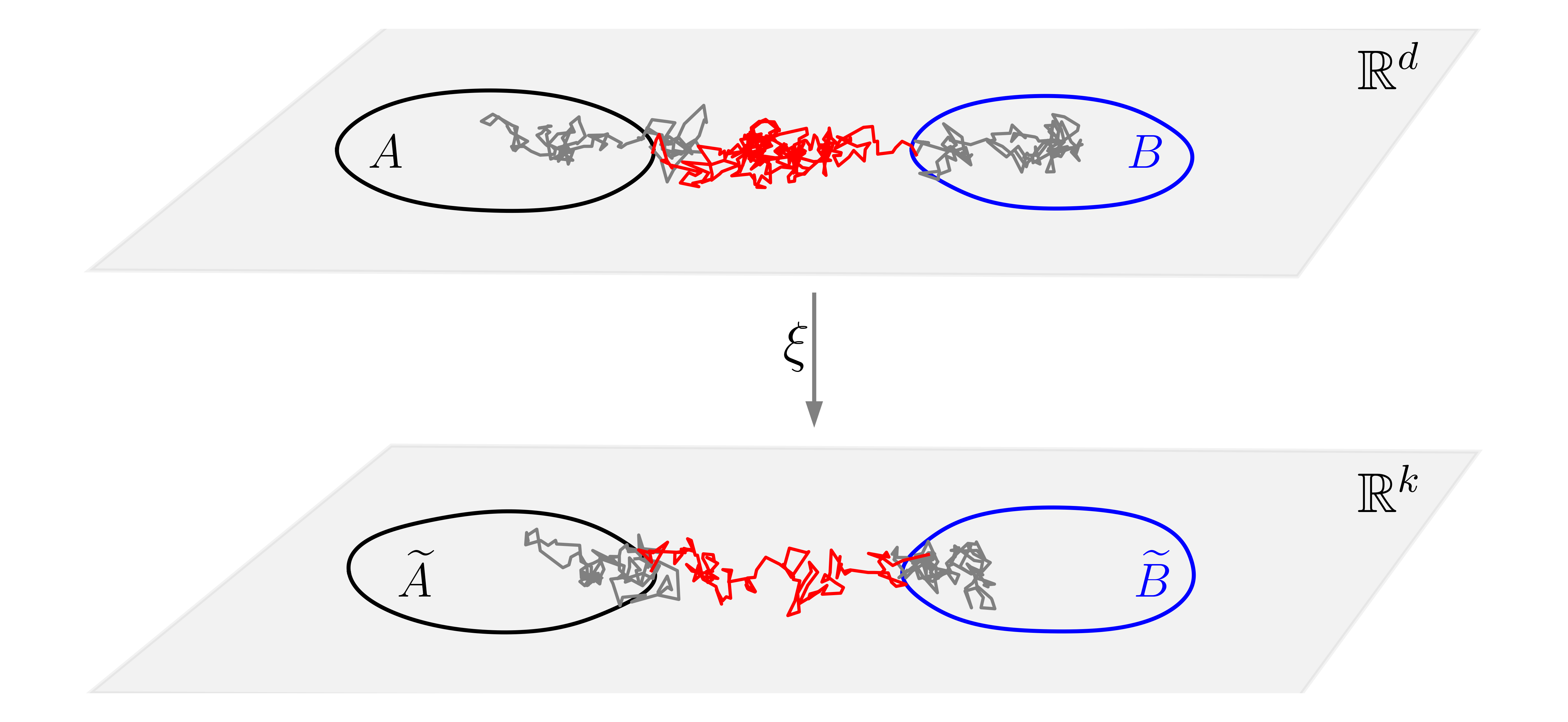
Let us assume that $A,B\subset\mathbb{R}^{d}$ are two closed subsets with smooth boundaries $\partial A$ and $\partial B$, respectively, such that $A\cap B=\emptyset$ and the complement of their union is nonempty, i.e. $(A\cup B)^{c}:=\mathbb{R}^{d}\setminus(A\cup B)\neq\emptyset$. Recall that TPT focuses on the reactive segments in the trajectory of $X_{n}$. Specifically, a trajectory segment $X_{m},X_{m+1},\dots,X_{m+j}$, where $m\geq 0$ and $j\geq 1$, is called reactive, if it starts from a state in $A$ and it goes to $B$ without returning to $A$, or equivalently, if $X_{m}\in A$, $X_{m+j}\in B$, and $X_{i}\in(A\cup B)^{c}$ for all $m<i<m+j$. See Figure 2 for illustration. Suppose that an infinitely long trajectory of $X_{n}$ is given and let $M_{N}^{R}$ denote the number of reactive segments that occur within the first $N$ steps of the trajectory (the last reactive segment is allowed to end after the $N$th step). Then, the transition rate of the process $X_{n}$ from $A$ to $B$ is defined as

$$k_{AB}=\lim_{N\rightarrow+\infty}\frac{M_{N}^{R}}{N}\,.$$ (31)

Let us also recall the so-called (forward) committor $q$ associated to the sets $A$ and $B$, which is defined by

$$q(x)=\mathbb{P}(\text{starting from $x$, $X_{n}$ enters $B$ before it enters $A$}),\quad x\in\mathbb{R}^{d}\,,$$ (32)

and satisfies the equation

$\displaystyle(\mathcal{T}q)(x)=q(x),\quad\forall~{}x\in(A\cup B)^{c}\,,$ (33)
$\displaystyle q|_{A}\equiv 0,\quad q|_{B}\equiv 1\,,$

where $\mathcal{T}$ is the transfer operator of the process $X_{n}$.

In the following, we give alternative expressions for the transition rate $k_{AB}$.

Proposition 3.

Let $p(x,y)$ be the transition density of $X_{n}$ and $\mathcal{E}$ be the Dirichlet energy defined in (11). Then, the following identities hold.

  1. 1.

    $k_{AB}=k_{BA}$.

  2. 2.

    $k_{AB}=\int_{A}\Big{[}\int_{\mathbb{R}^{d}}p(x,y)q(y)\,\mathrm{d}{y}\Big{]}\pi(x)\,\mathrm{d}{x}=\int_{B}\Big{[}\int_{\mathbb{R}^{d}}p(x,y)(1-q(y))\,\mathrm{d}{y}\Big{]}\pi(x)\,\mathrm{d}{x}$.

  3. 3.

    $k_{AB}=\mathcal{E}(q)=\frac{1}{2}\int_{\mathbb{R}^{d}}\int_{\mathbb{R}^{d}}p(x,y)|q(y)-q(x)|^{2}\pi(x)\,\mathrm{d}{x}\,\mathrm{d}{y}$.

Proof.

The first identity follows immediately from the definition (31) and the observation that between two consecutive reactive segments from $A$ to $B$ there is exactly one reactive segment from $B$ to $A$.

Concerning the second claim, we notice that the number of reactive segments within the first $N$ steps can be written as

$$M_{N}^{R}=\sum_{m=0}^{N-1}\mathbbm{1}_{A}(X_{m})\mathbbm{1}_{B}(X_{m+j_{m}})\,,$$

where $\mathbbm{1}_{A}$ (resp. $\mathbbm{1}_{B}$) denotes the indicator function of subset $A$ (resp. $B$), and $j_{m}:=\inf\{i\geq 1;X_{m+i}\in A\cup B\}$. Therefore, by the definition (31), we have

$$k_{AB}=\lim_{N\rightarrow+\infty}\frac{1}{N}\sum_{m=0}^{N-1}\mathbbm{1}_{A}(X_{m})\mathbbm{1}_{B}(X_{m+j_{m}})=\int_{A}\Big{[}\int_{\mathbb{R}^{d}}p(x,y)q(y)\,\mathrm{d}{y}\Big{]}\pi(x)\,\mathrm{d}{x}\,,$$

where the second equality follows from the definition of the committor $q$ in (32) and the ergodicity of the process $X_{n}$. Similarly, by considering reactive segments from $B$ to $A$ and applying the identity in the first claim, we obtain the second equality in this claim, since

$\displaystyle k_{AB}=k_{BA}=$ $\displaystyle\lim_{N\rightarrow+\infty}\frac{1}{N}\sum_{m=0}^{N-1}\mathbbm{1}_{B}(X_{m})\mathbbm{1}_{A}(X_{m+j_{m}})$ (34)
$\displaystyle=$ $\displaystyle\int_{B}\Big{[}\int_{\mathbb{R}^{d}}p(x,y)(1-q(y))\mathrm{d}{y}\Big{]}\pi(x)\,\mathrm{d}{x}\,.$

Concerning the third claim, from (11) we can compute

$\displaystyle\mathcal{E}(q)=$ $\displaystyle\frac{1}{2}\int_{\mathbb{R}^{d}}\int_{\mathbb{R}^{d}}p(x,y)|q(y)-q(x)|^{2}\pi(x)\,\mathrm{d}{x}\,\mathrm{d}{y}$
$\displaystyle=$ $\displaystyle\langle q,(\mathcal{I}-\mathcal{T})q\rangle_{\mu}$
$\displaystyle=$ $\displaystyle\int_{A}q(x)[(\mathcal{I}-\mathcal{T})q](x)\pi(x)\mathrm{d}{x}+\int_{(A\cup B)^{c}}q(x)[(\mathcal{I}-\mathcal{T})q](x)\pi(x)\,\mathrm{d}{x}$
$\displaystyle+\int_{B}q(x)[(\mathcal{I}-\mathcal{T})q](x)\pi(x)\,\mathrm{d}{x}$
$\displaystyle=$ $\displaystyle\int_{B}[(\mathcal{I}-\mathcal{T})q](x)\pi(x)\,\mathrm{d}{x}$
$\displaystyle=$ $\displaystyle\int_{B}\pi(x)\,\mathrm{d}{x}-\int_{B}\Big{[}\int_{\mathbb{R}^{d}}p(x,y)q(y)\,\mathrm{d}{y}\Big{]}\pi(x)\,\mathrm{d}{x}$
$\displaystyle=$ $\displaystyle\int_{B}\Big{[}\int_{\mathbb{R}^{d}}p(x,y)(1-q(y))\,\mathrm{d}{y}\Big{]}\pi(x)\,\mathrm{d}{x}$
$\displaystyle=$ $\displaystyle k_{AB}\,,$

where the second equality follows from (12) in Lemma 13 and the fact that $\langle f,(\mathcal{I}-\mathcal{T}^{rev})g\rangle_{\mu}=\langle f,(\mathcal{I}-\mathcal{T})g\rangle_{\mu}$ when $f=g$, the fourth equality follows by using the equation (33) of the committor $q$, the fifth equality follows from the definition of $\mathcal{T}$ and $f|_{B}\equiv 1$, the sixth equality follows from the fact that $\int_{\mathbb{R}^{d}}p(x,y)\mathrm{d}{y}=1$, and the last equality follows from (34). ∎

It is worth mentioning that Proposition 3 also holds for nonreversible ergodic Markov processes. In particular, the third claim of Proposition 3 states that the transition rate $k_{AB}$ equals to the Dirichlet energy of the committor $q$. In the reversible setting (see (9)), we can further obtain the following variational characterization of the committor.

Proposition 4.

Assume that $X_{n}$ is reversible. Let $q$ be the committor (32) associated to the transitions of $X_{n}$ from $A$ to $B$, and let $\mathcal{E}$ denote the Dirichlet energy defined in (11). For any function $f:\mathbb{R}^{d}\rightarrow\mathbb{R}$ satisfying

$$f|_{A}\equiv 0,\quad f|_{B}\equiv 1,$$ (35)

we have

$$\mathcal{E}(f)=k_{AB}+\mathcal{E}(f-q)\,.$$ (36)

In particular, $q$ solves the minimization problem

$$\min_{f}\mathcal{E}(f)$$ (37)

among all functions $f:\mathbb{R}^{d}\rightarrow\mathbb{R}$ satisfying the condition (35), and the minimum value is $k_{AB}$.

Proof.

It suffices to prove (36). Let us derive

$\displaystyle\mathcal{E}(f)=$ $\displaystyle\langle f,(\mathcal{I}-\mathcal{T})f\rangle_{\mu}$
$\displaystyle=$ $\displaystyle\big{\langle}q+(f-q),(\mathcal{I}-\mathcal{T})\big{(}q+(f-q)\big{)}\big{\rangle}_{\mu}$
$\displaystyle=$ $\displaystyle\langle q,(\mathcal{I}-\mathcal{T})q\rangle_{\mu}+\langle f-q,(\mathcal{I}-\mathcal{T})(f-q)\rangle_{\mu}+2\langle q,(\mathcal{I}-\mathcal{T})(f-q)\rangle_{\mu}$
$\displaystyle=$ $\displaystyle\mathcal{E}(q)+\mathcal{E}(f-q)+2\langle(\mathcal{I}-\mathcal{T})q,f-q\rangle_{\mu}$
$\displaystyle=$ $\displaystyle k_{AB}+\mathcal{E}(f-q)\,,$

where the first, the third, and the fourth equalities follow from (12) in Lemma 13 and the self-adjointness of $\mathcal{T}$, the last equality follows from the third claim of Proposition 3, the fact that $f\equiv q$ on $A\cup B$ thanks to the condition (35) (which is met by both $f$ and $q$), as well as the identity $(\mathcal{I}-\mathcal{T})q=0$ on $(A\cup B)^{c}$ as stated in the equation (33). ∎

Similar to Theorem 2.3 which concerns the leading eigenfunctions, we have the following characterization of the committor as a slow variable for the study of transitions from $A$ to $B$. We also refer to Remark 4.2 for discussions on a numerical approach (based on Proposition 4 and the effective dynamics in the next section) for learning CV maps that can parametrize the committor.

Theorem 2.4.

Assume that $X_{n}$ is reversible. Given two disjoint subsets $A,B\subset\mathbb{R}^{d}$, the CV map defined by the committor $q$ minimizes the average of squared variations

$$\min_{f}\lim_{N\rightarrow+\infty}\frac{1}{2N}\sum_{n=0}^{N-1}|f(X_{n+1})-f(X_{n})|^{2}$$

among all functions $f:\mathbb{R}^{d}\rightarrow\mathbb{R}$ which satisfy $f|_{A}\equiv 0$ and $f|_{B}\equiv 1$.

Proof.

The conclusion follows directly from Proposition 4 and Lemma 13. ∎

3 Effective dynamics for a given CV map

In this section, we study the effective dynamics of $X_{n}$ for a given CV map. We give the definition of the effective dynamics in Section 3.1 and then study its properties in Section 3.2. In particular, we show that its transition density can be characterized via a relative entropy minimization to the transition density of $X_{n}$ and discuss the application of this fact in finding CVs (see Proposition 6 and Remark 3.2).

3.1 Definitions

Before we define the effective dynamics for $X_{n}$, we need to introduce several useful quantities associated to the CV map. To keep the discussions concise and easy to follow, we will adopt the Dirac delta function and work with informal definitions at some places. We point out that all the quantities below can be defined in a rigorous manner (see Remark 3.1).
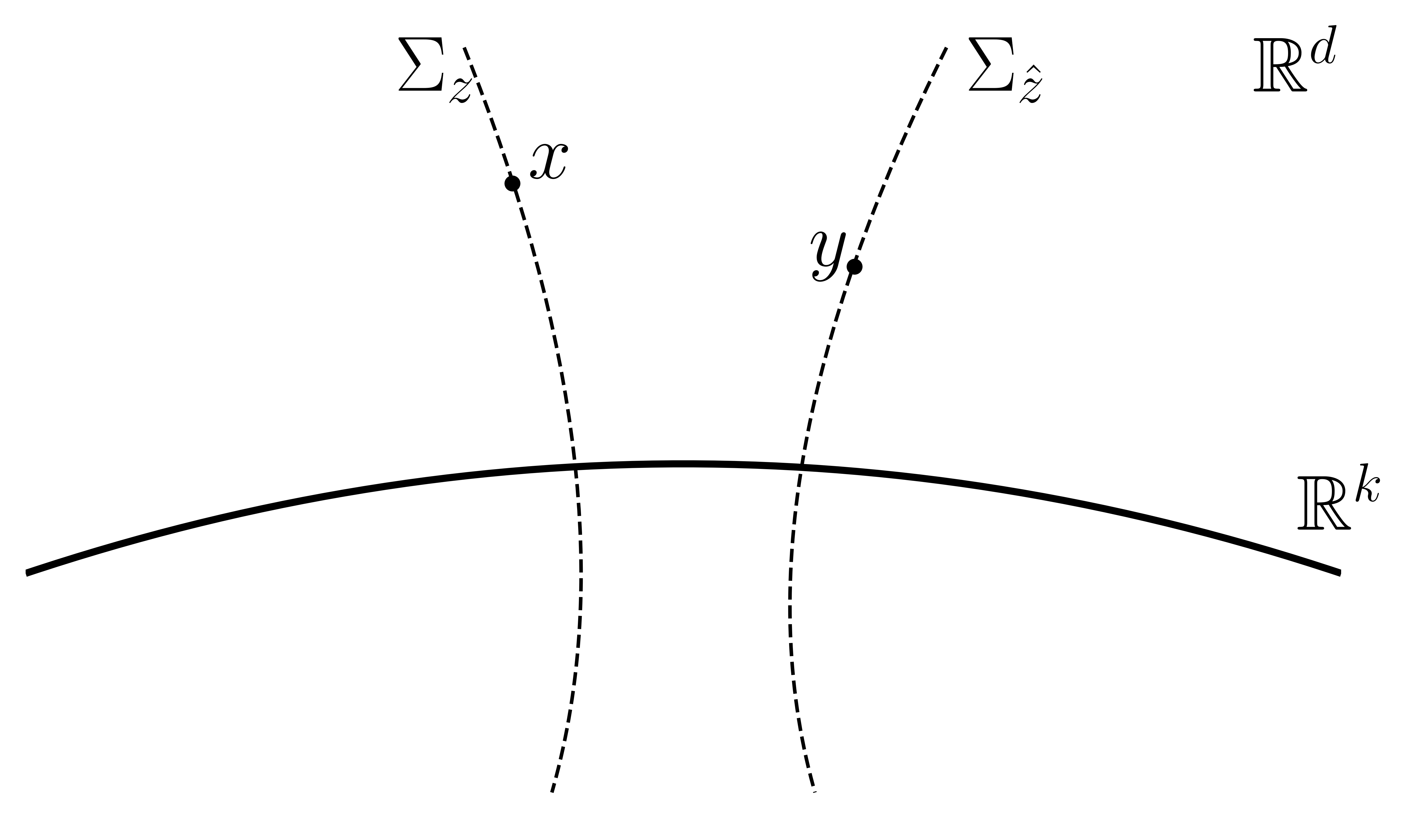
Let us assume that a $C^{2}$-smooth map $\xi=(\xi_{1},\xi_{2},\dots,\xi_{k})^{\top}:\mathbb{R}^{d}\rightarrow\mathbb{R}^{k}$ is given, where $1\leq k<d$ and $\xi_{i}:\mathbb{R}^{d}\rightarrow\mathbb{R}$ for $i=1,2,\dots,k$. Under certain conditions on $\xi$ (in particular, we assume $\xi$ is a onto map; see [30, 29] for concrete conditions), the level set

$$\Sigma_{z}:=\{x\in\mathbb{R}^{d},\xi(x)=z\}\,,$$ (38)

for a given $z\in\mathbb{R}^{k}$, is a $(d-k)$-dimensional submanifold in $\mathbb{R}^{d}$ (Figure 1). Given the map $\xi$, the so-called conditional probability measure $\mu_{z}$ on $\Sigma_{z}$ can be defined as

$$\mu_{z}(\mathrm{d}{x})=\frac{1}{Q(z)}\pi(x)\delta(\xi(x)-z)\,\mathrm{d}{x}\,,$$ (39)

where $\delta(\cdot)$ denotes the Dirac delta function and $Q(z)$ is a normalizing constant given by

$$Q(z)=\int_{\mathbb{R}^{d}}\pi(x)\delta(\xi(x)-z)\,\mathrm{d}{x}\,.$$ (40)

We also define the measure $\widetilde{\mu}$ on $\mathbb{R}^{k}$ (i.e. the pushforward measure of $\mu$ by $\xi$) by

$$\widetilde{\mu}(\mathrm{d}{z})=Q(z)\mathrm{d}{z}\,,\quad z\in\mathbb{R}^{k}\,.$$ (41)

The fact that $\widetilde{\mu}$ is a probability measure can be verified using the well-known identity involving the Dirac delta function:

$$\int_{\mathbb{R}^{k}}\bigg{[}\int_{\mathbb{R}^{d}}f(x)\delta(\xi(x)-\hat{z})\,\mathrm{d}{x}\bigg{]}\,\mathrm{d}{\hat{z}}=\int_{\mathbb{R}^{d}}f(x)\,\mathrm{d}{x}\,,\quad f:\mathbb{R}^{d}\rightarrow\mathbb{R}~{}\mathrm{is~{}integrable}\,.$$ (42)

To motivate the definition of effective dynamics, let us point out that $\xi(X_{n})$ is in general a non-Markovian process in $\mathbb{R}^{k}$, since the probability that $\xi(X_{n+1})\in\widetilde{D}$ at $(n+1)$th step for a subset $\widetilde{D}\subset\mathbb{R}^{k}$ depends on the full state $X_{n}=x$ at $n$th step rather than $\xi(X_{n})=z$ only, i.e.

$$\mathbb{P}(\xi(X_{n+1})\in\widetilde{D}|X_{n}=x)=\int_{\widetilde{D}}\int_{\mathbb{R}^{d}}p(x,y)\delta(\xi(y)-\hat{z})\,\mathrm{d}{y}\,\mathrm{d}{\hat{z}}\,.$$ (43)

One way to define a transition density in $\mathbb{R}^{k}$ is to take average on the right hand side of (43) over the states $X_{n}=x$ on $\Sigma_{z}$ with respect to the conditional measure $\mu_{z}$ in (39). Specifically, given the CV map $\xi$, we define the effective dynamics of $X_{n}$ as follows.

Definition 1 (Effective dynamics).

The effective dynamics of $X_{n}$ associated to the CV map $\xi:\mathbb{R}^{d}\rightarrow\mathbb{R}^{k}$ is defined as the Markov process $Z_{n}$ in $\mathbb{R}^{k}$ with the transition density $\widetilde{p}(z,\hat{z})$, where

$\displaystyle\widetilde{p}(z,\hat{z})=$ $\displaystyle\int_{\Sigma_{z}}\Big{[}\int_{\mathbb{R}^{d}}p(x,y)\delta(\xi(y)-\hat{z})\,\mathrm{d}{y}\Big{]}\,\mu_{z}(\mathrm{d}{x})$ (44)
$\displaystyle=$ $\displaystyle\frac{1}{Q(z)}\int_{\mathbb{R}^{d}}\int_{\mathbb{R}^{d}}p(x,y)\delta(\xi(x)-z)\delta(\xi(y)-\hat{z})\pi(x)\,\mathrm{d}{x}\,\mathrm{d}{y},\quad z,\hat{z}\in\mathbb{R}^{k}\,.$

Using (42) and the fact that $p(x,\cdot)$ is a probability density in $\mathbb{R}^{d}$, we can verify that $\widetilde{p}(z,\cdot)$ in (44) indeed defines a probability density for $z\in\mathbb{R}^{k}$, i.e. $\int_{\mathbb{R}^{k}}\widetilde{p}(z,\hat{z})\,\mathrm{d}{\hat{z}}=1$. As we show in the next subsection, Definition 44 is very natural, because the invariant distribution of $Z_{n}$ is directly related to the free energy associated to $\xi$ [28] and its transition density $\widetilde{p}$ gives the best approximation of $p$ in the sense of relative entropy minimization [7, Section 2.3].

We conclude this section with a discussion on how to make the definitions above rigorous.

Remark 3.1 (Rigorous definitions).

The conditional probability measure $\mu_{z}$ in (39) and the normalizing constant $Q(z)$ in (40) can be defined rigorously without using the Dirac delta function. See (85) and (86) in Appendix B, respectively. In particular, using co-area formula [12, Theorem 3.11], the transition density in (44) can be written rigorously as

$$\widetilde{p}(z,\hat{z})=\int_{\Sigma_{z}}\int_{\Sigma_{\hat{z}}}p(x,y)\big{[}\mathrm{det}(\nabla\xi(y)\nabla\xi(y)^{\top})\big{]}^{-\frac{1}{2}}\,\mu_{z}(\mathrm{d}{x})\,\sigma_{\Sigma_{\hat{z}}}(\mathrm{d}{y}),\quad z,\hat{z}\in\mathbb{R}^{k}\,,$$ (45)

where $\sigma_{\Sigma_{\hat{z}}}$ denotes the surface measure on $\Sigma_{\hat{z}}$, $\nabla\xi(y)\in\mathbb{R}^{k\times d}$ denotes the Jacobian matrix of $\xi$ at $y$, and $\mathrm{det}(\nabla\xi(y)\nabla\xi(y)^{\top})$ denotes the determinant of the $k\times k$ matrix $\nabla\xi(y)\nabla\xi(y)^{\top}$.

Refer to caption
Figure 1: Illustration of level sets of the CV map $\xi:\mathbb{R}^{d}\rightarrow\mathbb{R}^{k}$ for values $z,\hat{z}\in\mathbb{R}^{k}$.

3.2 Properties of effective dynamics

In this section, we study properties of the effective dynamics $Z_{n}$ in Definition 44 whose transition density $\widetilde{p}$ is defined in (44). Let us first identify its invariant probability measure.

Proposition 5.

The probability measure $\widetilde{\mu}$ defined in (41) is an invariant measure of $Z_{n}$.

Proof.

To show the invariance of $\widetilde{\mu}$, let us compute, for $\hat{z}\in\mathbb{R}^{k}$,

$\displaystyle\int_{\mathbb{R}^{k}}\widetilde{p}(z,\hat{z})\,Q(z)\,\mathrm{d}{z}$
$\displaystyle=$ $\displaystyle\int_{\mathbb{R}^{k}}\bigg{[}\frac{1}{Q(z)}\int_{\mathbb{R}^{d}}\int_{\mathbb{R}^{d}}p(x,y)\delta(\xi(x)-z)\delta(\xi(y)-\hat{z})\pi(x)\,\mathrm{d}{x}\,\mathrm{d}{y}\bigg{]}\,Q(z)\,\mathrm{d}{z}$
$\displaystyle=$ $\displaystyle\int_{\mathbb{R}^{k}}\bigg{[}\int_{\mathbb{R}^{d}}\int_{\mathbb{R}^{d}}p(x,y)\delta(\xi(x)-z)\delta(\xi(y)-\hat{z})\pi(x)\,\mathrm{d}{x}\,\mathrm{d}{y}\bigg{]}\,\mathrm{d}{z}$
$\displaystyle=$ $\displaystyle\int_{\mathbb{R}^{d}}\int_{\mathbb{R}^{d}}p(x,y)\delta(\xi(y)-\hat{z})\pi(x)\,\mathrm{d}{x}\,\mathrm{d}{y}$
$\displaystyle=$ $\displaystyle\int_{\mathbb{R}^{d}}\pi(y)\delta(\xi(y)-\hat{z})\,\mathrm{d}{y}$
$\displaystyle=$ $\displaystyle Q(\hat{z})\,,$

where the first equality follows from (44) and (41), the third equality follows from (42), the fourth equality follows from the invariance of $\pi$ in (1), and the last equality follows from the definition of $Q$ in (40). ∎

From now on, we will assume that the effective dynamics $Z_{n}$ is ergodic and $\widetilde{\mu}$ is its unique invariant probability measure. Notice that the free energy associated to the CV map $\xi$, denoted by the map $F:\mathbb{R}^{k}\rightarrow\mathbb{R}$, is related to the normalizing constant in (40) by $F(z)=-\beta^{-1}\ln Q(z)$ [28], where $\beta>0$ is a constant related to the system’s temperature. Therefore, Proposition 5 states that $Z_{n}$ as a surrogate model has the desired invariant probability measure whose density is $Q(z)=\exp(-\beta F(z))$, for $z\in\mathbb{R}^{k}$.

In the following, we present a variational characterization of the transition density $\widetilde{p}$ of $Z_{n}$ by showing that $\widetilde{p}$, together with the conditional measure $\mu_{z}$, gives the best approximation of $p$ within certain class of transition densities in terms of relative entropy minimization. To this end, note that the transition density $p$ can be written as

$$p(x,y)=p(\hat{z}|x)\,p(y|\hat{z},x),$$ (46)

where $p(\hat{z}|x)$ denotes the probability density of $\hat{z}=\xi(y)\in\mathbb{R}^{k}$ given the value $x\in\mathbb{R}^{d}$, and $p(y|\hat{z},x)$ is the probability density of $y\in\Sigma_{\hat{z}}$ given the values $\hat{z}$ and $x$ (see Figure 1 for illustration). Finding a Markov process on $\mathbb{R}^{k}$ that mimics the dynamics of $\xi(X_{n})$ can be achieved by considering the approximation of $p$ within the set $\Theta^{\xi}$ of probability densities $\bar{p}$, which have the following form

$$\bar{p}(x,y)=g(\xi(x),\hat{z})\,\bar{p}_{\hat{z}}(y),\quad x,y\in\mathbb{R}^{d},\quad\xi(y)=\hat{z}\in\mathbb{R}^{k}\,,$$ (47)

where $g$ is a transition density function on $\mathbb{R}^{k}$ and $\bar{p}_{\hat{z}}$ is a probability density on the level set $\Sigma_{\hat{z}}$ (with respect to its surface measure $\sigma_{\Sigma_{\hat{z}}}$). In other words, we approximate the two terms on the right hand side of (46) by assuming that the first term is only conditioned on $z=\xi(x)$ rather than $x$ and the second term only on $\hat{z}$.

The following result states that, among the probability densities in (47), the one which minimizes the relative entropy (or, KL-divergence) to $p$ is given by the transition density $\widetilde{p}$ (44) of the effective dynamics $Z_{n}$ in Definition 44 and the conditional expectation $\mu_{z}$ (39) (see (85) in Appendix B for the density of $\mu_{z}$ and also Remark 3.1 for discussions).

Proposition 6.

For $z\in\mathbb{R}^{k}$, let $p_{z}$ be the density of $\mu_{z}$ on $\Sigma_{z}$ with respect to $\sigma_{\Sigma_{z}}$, i.e. $p_{z}=\frac{\mathrm{d}{}\mu_{z}}{\mathrm{d}{}\sigma_{\Sigma_{z}}}$. For fixed $x\in\mathbb{R}^{d}$, denote by $D_{\mathrm{KL}}(p(x,\cdot)\|\bar{p}(x,\cdot))$ the KL-divergence from the density $\bar{p}(x,\cdot)$ to the density $p(x,\cdot)$. Then the minimizer

$$\bar{p}^{*}=\arg\min_{\bar{p}\in\Theta^{\xi}}\mathbb{E}_{x\sim\mu}\Big{(}D_{\mathrm{KL}}\big{(}p(x,\cdot)\,\|\,\bar{p}(x,\cdot)\big{)}\Big{)}$$ (48)

is given by (47) with $g=\widetilde{p}$ and $\bar{p}_{z}=p_{z}$ for $z\in\mathbb{R}^{k}$.

Proof.

By definition of KL-divergence [7, Section 2.3], we have, for $\bar{p}\in\Theta^{\xi}$,

$\displaystyle\begin{split}&\mathbb{E}_{x\sim\mu}\Big{(}D_{\mathrm{KL}}\big{(}p(x,\cdot)\,\|\,\bar{p}(x,\cdot)\big{)}\Big{)}\\ =&\int_{\mathbb{R}^{d}}\bigg{[}\int_{\mathbb{R}^{d}}p(x,y)\ln\frac{p(x,y)}{\bar{p}(x,y)}\,\mathrm{d}{y}\bigg{]}\pi(x)\,\mathrm{d}{x}\\ =&\int_{\mathbb{R}^{d}}\bigg{[}\int_{\mathbb{R}^{d}}p(x,y)\ln p(x,y)\,\mathrm{d}{y}\bigg{]}\pi(x)\,\mathrm{d}{x}-\int_{\mathbb{R}^{d}}\bigg{[}\int_{\mathbb{R}^{d}}p(x,y)\ln\bar{p}(x,y)\,\mathrm{d}{y}\bigg{]}\pi(x)\,\mathrm{d}{x}\,,\end{split}$ (49)

where the first term in the last line is independent of $\bar{p}$. For the second term, we can derive

$\displaystyle-\int_{\mathbb{R}^{d}}\bigg{[}\int_{\mathbb{R}^{d}}p(x,y)\ln\bar{p}(x,y)\,\mathrm{d}{y}\bigg{]}\pi(x)\,\mathrm{d}{x}$
$\displaystyle=$ $\displaystyle-\int_{\mathbb{R}^{d}}\bigg{[}\int_{\mathbb{R}^{d}}p(x,y)\big{(}\ln g(\xi(x),\xi(y))+\ln\bar{p}_{\xi(y)}(y)\big{)}\,\mathrm{d}{y}\bigg{]}\pi(x)\,\mathrm{d}{x}$
$\displaystyle=$ $\displaystyle-\int_{\mathbb{R}^{k}}\bigg{[}\int_{\mathbb{R}^{k}}\widetilde{p}(z,\hat{z})\ln g(z,\hat{z})\,\mathrm{d}{\hat{z}}\bigg{]}Q(z)\,\mathrm{d}{z}-\int_{\mathbb{R}^{d}}\bigg{[}\int_{\mathbb{R}^{d}}p(x,y)\ln\bar{p}_{\xi(y)}(y)\,\mathrm{d}{y}\bigg{]}\pi(x)\,\mathrm{d}{x}$
$\displaystyle=$ $\displaystyle-\int_{\mathbb{R}^{k}}\bigg{[}\int_{\mathbb{R}^{k}}\widetilde{p}(z,\hat{z})\ln g(z,\hat{z})\,\mathrm{d}{\hat{z}}\bigg{]}Q(z)\,\mathrm{d}{z}-\int_{\mathbb{R}^{d}}\ln\bar{p}_{\xi(x)}(x)\,\pi(x)\,\mathrm{d}{x}$
$\displaystyle=$ $\displaystyle-\int_{\mathbb{R}^{k}}\bigg{[}\int_{\mathbb{R}^{k}}\widetilde{p}(z,\hat{z})\ln g(z,\hat{z})\,\mathrm{d}{\hat{z}}+\int_{\Sigma_{z}}\ln\bar{p}_{z}(x)\mu_{z}(\mathrm{d}{x})\bigg{]}Q(z)\,\mathrm{d}{z}$
$\displaystyle=$ $\displaystyle\int_{\mathbb{R}^{k}}\bigg{[}D_{\mathrm{KL}}\big{(}\widetilde{p}(z,\cdot)\,\|\,g(z,\cdot)\big{)}+D_{\mathrm{KL}}(p_{z}\,\|\,\bar{p}_{z})\bigg{]}Q(z)\,\mathrm{d}{z}$
$\displaystyle-\int_{\mathbb{R}^{k}}\bigg{[}\int_{\mathbb{R}^{k}}(\widetilde{p}\ln\widetilde{p})(z,\hat{z})\,\mathrm{d}{\hat{z}}+\int_{\Sigma_{z}}\ln p_{z}(x)\mu_{z}(\mathrm{d}{x})\bigg{]}Q(z)\,\mathrm{d}{z}\,,$ (50)

where the first equality follows from the expression of $\bar{p}$ in (47), the second equality follows by applying the identity (42) and the definition of $\widetilde{p}$ in (44), the third equality follows from the invariance of $\pi$ in (1), the fourth equality follows by applying the identity (42) and the definition of $\mu_{z}$ in (39), and finally the last equality follows from the definition of KL-divergence.

Putting (49) and (50) together, we get, for any $\bar{p}\in\Theta^{\xi}$,

$\displaystyle\begin{split}&\mathbb{E}_{x\sim\mu}\Big{(}D_{\mathrm{KL}}\big{(}p(x,\cdot)\,\|\,\bar{p}(x,\cdot)\big{)}\Big{)}\\ =&\int_{\mathbb{R}^{k}}\bigg{[}D_{\mathrm{KL}}\big{(}\widetilde{p}(z,\cdot)\,\|\,g(z,\cdot)\big{)}+D_{\mathrm{KL}}(p_{z}\,\|\,\bar{p}_{z})\bigg{]}Q(z)\,\mathrm{d}{z}\\ &-\int_{\mathbb{R}^{k}}\bigg{[}\int_{\mathbb{R}^{k}}(\widetilde{p}\ln\widetilde{p})(z,\hat{z})\,\mathrm{d}{\hat{z}}+\int_{\Sigma_{z}}\ln p_{z}(x)\mu_{z}(\mathrm{d}{x})\bigg{]}Q(z)\,\mathrm{d}{z}\\ &+\int_{\mathbb{R}^{d}}\bigg{[}\int_{\mathbb{R}^{d}}p(x,y)\ln p(x,y)\,\mathrm{d}{y}\bigg{]}\pi(x)\,\mathrm{d}{x}\,.\end{split}$ (51)

Since $\bar{p}$ is only involved (through $g$ and $\bar{p}_{z}$) in the first integral on the right hand side of (51) and the KL-divergence is nonnegative and it equals to zero if and only if the two densities are identical, we conclude that the objective in (48) is minimized when $\bar{p}$ is given in (47) with $g=\widetilde{p}$ and $\bar{p}_{z}=p_{z}$ for $z\in\mathbb{R}^{k}$. ∎

Proposition 6 shows that, given the CV map $\xi$, the effective dynamics $Z_{n}$ in Definition 44 with the transition density $\widetilde{p}$ in (44) is the optimal surrogate model in the sense of relative entropy minimization (47)–(48). But, apparently the ability of $Z_{n}$ in approximating/representing the true dynamics $X_{n}$ depends on the choice of $\xi$. In Section 4 we will study the approximation quality of $Z_{n}$ in terms of estimating both the spectrum and transition rates of the true dynamics $X_{n}$. We note that conditions on the choice of $\xi$ which gives a good effective dynamics have been investigated in the transition manifold framework [2, 3].

In the following result, we transform Proposition 6 into variational formulations that allow for optimizing the CV map $\xi$.

Theorem 3.1 (Optimizing CV maps by relative entropy minimization).

The CV map $\xi$ with the least KL-divergence between the full dynamics and the effective dynamics solves the following equivalent optimization tasks:

$\displaystyle\min_{\xi}\min_{\bar{p}\in\Theta^{\xi}}\mathbb{E}_{x\sim\mu}\Big{(}D_{\mathrm{KL}}\big{(}p(x,\cdot)\,\|\,\bar{p}(x,\cdot)\big{)}\Big{)}$ (52)
$\displaystyle\Longleftrightarrow$ $\displaystyle\min_{\xi,g,\bar{p}_{z}}\bigg{[}-\int_{\mathbb{R}^{d}}\Big{[}\int_{\mathbb{R}^{d}}p(x,y)\ln g(\xi(x),\xi(y))\,\mathrm{d}{y}\Big{]}\pi(x)\,\mathrm{d}{x}-\int_{\mathbb{R}^{d}}\ln\bar{p}_{\xi(x)}(x)\pi(x)\,\mathrm{d}{x}\bigg{]}$ (53)
$\displaystyle\Longleftrightarrow$ $\displaystyle\min_{\xi,g}\bigg{[}-\int_{\mathbb{R}^{d}}\Big{[}\int_{\mathbb{R}^{d}}p(x,y)\ln g(\xi(x),\xi(y))\,\mathrm{d}{y}\Big{]}\pi(x)\,\mathrm{d}{x}+\max_{\bar{Q}}\int_{\mathbb{R}^{d}}\ln\bar{Q}(\xi(x))\pi(x)\,\mathrm{d}{x}$
$\displaystyle\hskip 34.14322pt+\frac{1}{2}\int_{\mathbb{R}^{d}}\ln\mathrm{det}(\nabla\xi(x)\nabla\xi(x)^{\top})\pi(x)\,\mathrm{d}{x}\bigg{]}\,,$ (54)

where $g$ is a transition density on $\mathbb{R}^{k}$, $\bar{p}_{z}$ is a probability density on $\Sigma_{z}$, and $\bar{Q}$ is a probability density on $\mathbb{R}^{k}$ .

Proof.

The equivalence between (52) and (53) follows by rewriting (51) using (42) and noticing the fact that the last term there is independent of both $\xi$ and $\bar{p}$. By a similar argument, from (51) and using the fact that the divergence $D_{KL}(p_{z}\|\bar{p}_{z})$ vanishes when $\bar{p}_{z}=p_{z}$, we obtain that (52) is equivalent to

$$\min_{\xi,g}\bigg{[}-\int_{\mathbb{R}^{d}}\Big{[}\int_{\mathbb{R}^{d}}p(x,y)\ln g(\xi(x),\xi(y))\,\mathrm{d}{y}\Big{]}\,\pi(x)\,\mathrm{d}{x}-\int_{\mathbb{R}^{d}}\ln p_{\xi(x)}(x)\pi(x)\,\mathrm{d}{x}\bigg{]}\,.$$ (55)

To show the equivalence between (52) and (54), note that, using the expression of $D_{KL}(Q|\bar{Q})$ where $Q$ is the probability density on $\mathbb{R}^{k}$ defined in (40), we can verify that

$$\int_{\mathbb{R}^{d}}\ln Q(\xi(x))\pi(x)\,\mathrm{d}{x}=\max_{\bar{Q}}\int_{\mathbb{R}^{d}}\ln\bar{Q}(\xi(x))\pi(x)\,\mathrm{d}{x}.$$

Using the identity above and the expression of the density $p_{z}$ in (85), we can rewrite (55) as (54). This shows the equivalence between (52) and (54). ∎

Remark 3.2 (Algorithmic realization).

Theorem 3.1 provides two possible data-driven numerical approaches for jointly learning $\xi$ and the transition density $\widetilde{p}$ of the effective dynamics. (see [3] for alternative objective loss functions involving weighted $L^{1}$ norm of densities).

  1. 1.

    The first approach is to solve (52) (or (53)). It boils down to minimizing the negative log-likelihood with trajectory data $X_{0},X_{1},\dots,X_{N}$:

    $$\min_{\xi}\min_{\bar{p}\in\Theta^{\xi}}\Big{[}-\frac{1}{N}\sum_{n=0}^{N-1}\ln\bar{p}(X_{n},X_{n+1})\Big{]}\,.$$ (56)

    This recovers the loss function proposed in [51] for learning CV maps based on normalizing flows [23].

  2. 2.

    The second approach is to solve (54). With trajectory data, it amounts to solving

    $\displaystyle\begin{split}\min_{\xi}\Big{[}&-\max_{g}\frac{1}{N}\sum_{n=0}^{N-1}\ln g(\xi(X_{n}),\xi(X_{n+1}))+\max_{\bar{Q}}\frac{1}{N}\sum_{n=0}^{N-1}\ln\bar{Q}(\xi(X_{n}))\\ &+\frac{1}{2N}\sum_{n=0}^{N-1}\ln\mathrm{det}(\nabla\xi(X_{n})\nabla\xi(X_{n})^{\top})\Big{]}\,.\end{split}$ (57)

In (56), learning $\bar{p}$ requires to learn the densities $\bar{p}_{z}$ on (high-dimensional) level sets. In contrast, both $g$ and $\bar{Q}$ in (57) are functions in a low-dimensional space, i.e. $\mathbb{R}^{k}$. Hence, the second approach may have less complexity in comparison with the first approach.

Next, we study the transfer operator of the effective dynamics. In analogy to the transfer operator $\mathcal{T}$ of $X_{n}$ (see (2)), we define the transfer operator associated to $Z_{n}$ by

$$(\widetilde{\mathcal{T}}\widetilde{f}\,)(z)=\int_{\mathbb{R}^{k}}\widetilde{p}(z,\hat{z})\widetilde{f}(\hat{z})\,\mathrm{d}{\hat{z}}\,,\quad z\in\mathbb{R}^{k}$$ (58)

for functions in the Hilbert space

$$\widetilde{\mathcal{H}}=L^{2}_{\widetilde{\mu}}(\mathbb{R}^{k}):=\Big{\{}\widetilde{f}\,\Big{|}\,\widetilde{f}:\mathbb{R}^{k}\rightarrow\mathbb{R},\,\int_{\mathbb{R}^{k}}\widetilde{f}^{\,2}(z)\,Q(z)\,\mathrm{d}{z}<+\infty\Big{\}}\,,$$

which is endowed with the weighted inner product (the corresponding norm is denoted by $\|\cdot\|_{\widetilde{\mu}}$)

$$\langle\widetilde{f},\widetilde{g}\,\rangle_{\widetilde{\mu}}=\int_{\mathbb{R}^{k}}\widetilde{f}(z)\widetilde{g}(z)Q(z)\,\mathrm{d}{z}\,,\quad\widetilde{f},\widetilde{g}\in\widetilde{\mathcal{H}}\,.$$ (59)

The following lemma reveals the relations between the transfer operators $\widetilde{\mathcal{T}}$ and $\mathcal{T}$.

Lemma 2.

Let $\mathcal{T}$ be the transfer operator in (2) associated to $X_{n}$ and $\widetilde{\mathcal{T}}$ be the transfer operator in (58) associated to $Z_{n}$. Then, the following relations hold.

  1. 1.

    For any $\widetilde{g}\in\widetilde{\mathcal{H}}$, we have $(\widetilde{\mathcal{T}}\,\widetilde{g})(z)=\mathbb{E}_{\mu_{z}}(\mathcal{T}g)$ for all $z\in\mathbb{R}^{k}$, where $g=\widetilde{g}\circ\xi$ and $\mathbb{E}_{\mu_{z}}(\cdot)$ denotes the expectation with respect to $\mu_{z}$.

  2. 2.

    For any two functions $\widetilde{f},\widetilde{g}\in\widetilde{\mathcal{H}}$, we have $\langle\widetilde{\mathcal{T}}\widetilde{f},\widetilde{g}\rangle_{\widetilde{\mu}}=\langle\mathcal{T}f,g\rangle_{\mu}$, where $f=\widetilde{f}\circ\xi$ and $g=\widetilde{g}\circ\xi$.

Proof.

Concerning the first claim, given $\widetilde{g}\in\widetilde{\mathcal{H}}$, let us compute

$\displaystyle(\widetilde{\mathcal{T}}\,\widetilde{g})(z)=$ $\displaystyle\int_{\mathbb{R}^{k}}\widetilde{p}(z,\hat{z})\widetilde{g}(\hat{z})\,\mathrm{d}{\hat{z}}$
$\displaystyle=$ $\displaystyle\int_{\mathbb{R}^{k}}\bigg{[}\int_{\Sigma_{z}}\int_{\mathbb{R}^{d}}p(x,y)\delta(\xi(y)-\hat{z})\,\mathrm{d}{y}\,\mu_{z}(\mathrm{d}{x})\bigg{]}\widetilde{g}(\hat{z})\,\mathrm{d}{\hat{z}}$
$\displaystyle=$ $\displaystyle\int_{\Sigma_{z}}\int_{\mathbb{R}^{d}}p(x,y)\widetilde{g}(\xi(y))\,\mathrm{d}{y}\,\mu_{z}(\mathrm{d}{x})$
$\displaystyle=$ $\displaystyle\mathbb{E}_{\mu_{z}}(\mathcal{T}g)\,,$

where $g=\widetilde{g}\circ\xi$, and we have used (58), (44), as well as (42) to derive the above equalities. Concerning the second claim, using (39), (59), the first claim, and the identity (42), we can compute

$\displaystyle\langle\widetilde{\mathcal{T}}\,\widetilde{f},\widetilde{g}\rangle_{\widetilde{\mu}}=$ $\displaystyle\int_{\mathbb{R}^{k}}\big{(}\mathbb{E}_{\mu_{z}}(\mathcal{T}f)\big{)}\widetilde{g}(z)Q(z)\,\mathrm{d}{z}$
$\displaystyle=$ $\displaystyle\int_{\mathbb{R}^{k}}\bigg{[}\frac{1}{Q(z)}\int_{\mathbb{R}^{d}}(\mathcal{T}f)(x)\delta(\xi(x)-z)\pi(x)\,\mathrm{d}{x}\bigg{]}\widetilde{g}(z)Q(z)\,\mathrm{d}{z}$
$\displaystyle=$ $\displaystyle\int_{\mathbb{R}^{d}}(\mathcal{T}f)(x)\widetilde{g}(\xi(x))\pi(x)\,\mathrm{d}{x}$
$\displaystyle=$ $\displaystyle\langle\mathcal{T}f,g\rangle_{\mu}\,,$

where $f=\widetilde{f}\circ\xi$ and $g=\widetilde{g}\circ\xi$.

Using the above relation, we discuss in the following remark the relevance of effective dynamics to data-driven numerical algorithms in VAMP when the system’s features are employed.

Remark 3.3 (Relevance of effective dynamics in numerical algorithms).

Suppose that in applications the VAMP-r score is maximized in order to learn the $m$ leading eigenfunctions $(f_{i})_{1\leq i\leq m}$ of $\mathcal{T}$ (see Remark 2.3 and [50, 31]). Consider first the case $r=1$. Often, these eigenfunctions are represented as functions of system’s features, i.e. $f_{i}(x)=\widetilde{f}_{i}(\mathbf{R}(x))$, where $\widetilde{f}_{i}:\mathbb{R}^{K}\rightarrow\mathbb{R}$, integer $K\gg 1$, and $\mathbf{R}=(\mathbf{R}_{1},\dots,\mathbf{R}_{K})^{\top}:\mathbb{R}^{d}\rightarrow\mathbb{R}^{K}$ is a map describing $K$ features (i.e. feature map or internal variables) of the system $X_{n}$. Consider this specific CV map $\xi=\mathbf{R}$ and define the quantities in Section 3.1 accordingly. Using the second claim in Lemma 2, we obtain for the VAMP-1 score

$\displaystyle\sum_{i=1}^{m}\langle f_{i},\mathcal{T}f_{i}\rangle_{\mu}=\sum_{i=1}^{m}\langle\widetilde{f}_{i},\widetilde{\mathcal{T}}\widetilde{f}_{i}\rangle_{\widetilde{\mu}}\,,$ (60)

and the constraints in (26) are equivalent to

$\displaystyle\mathbb{E}_{\widetilde{\mu}}(\widetilde{f}_{i})=0,$ $\displaystyle\quad\forall\,i\,\in\{1,\dots,m\}\,,$ (61)
$\displaystyle\langle\widetilde{f}_{i},\widetilde{f}_{j}\rangle_{\widetilde{\mu}}=\delta_{ij}\,,$ $\displaystyle\quad\forall\,i,j\,\in\{1,\dots,m\}\,.$

In other words, approximating eigenfunctions of $\mathcal{T}$ by functions of system’s features is equivalent to approximating eigenfunctions of $\widetilde{\mathcal{T}}$ associated to the feature map $\mathbf{R}$. A similar conclusion holds for the case of VAMP-r score, where $r>1$, since we can obtain a similar identity as (60) by considering effective dynamics built with lag-time $r\tau$ and noticing that $\mathcal{T}^{r}$ is the transfer operator corresponding to the lag-time $r\tau$ (see Remark 2.3).

In the last part of this section, we discuss the reversibility of $Z_{n}$ and its connection to the reversibility of $X_{n}$. Denote by $\widetilde{\mathcal{T}}^{*}$ the adjoint of $\widetilde{\mathcal{T}}$ in $\widetilde{\mathcal{H}}$, which satisfies $\langle\widetilde{\mathcal{T}}\widetilde{f},\widetilde{g}\,\rangle_{\widetilde{\mu}}=\langle\widetilde{f},\widetilde{\mathcal{T}}^{*}\widetilde{g}\,\rangle_{\widetilde{\mu}}$ for any $\widetilde{f},\widetilde{g}\in\widetilde{\mathcal{H}}$. The following result gives the concrete expression of $\widetilde{\mathcal{T}}^{*}$.

Proposition 7.

For $\widetilde{f}\in\widetilde{\mathcal{H}}$, we have the following identity

$$(\widetilde{\mathcal{T}}^{*}\widetilde{f}\,)(z)=\int_{\mathbb{R}^{k}}\widetilde{p}^{*}(z,\hat{z})\widetilde{f}(\hat{z})\,\mathrm{d}{\hat{z}}\,,\quad z\in\mathbb{R}^{k}\,,$$ (62)

with the transition density

$$\widetilde{p}^{*}(z,\hat{z})=\frac{\widetilde{p}(\hat{z},z)Q(\hat{z})}{Q(z)}=\int_{\Sigma_{z}}\int_{\mathbb{R}^{d}}p^{*}(x,y)\delta(\xi(y)-\hat{z})\,\mathrm{d}{y}\,\mu_{z}(\mathrm{d}{x})\,,\quad z,\hat{z}\in\mathbb{R}^{k}\,,$$ (63)

where $p^{*}$ is given in (5).

Proof.

For any $\widetilde{f},\widetilde{g}\in\widetilde{\mathcal{H}}$, direct calculation gives

$\displaystyle\langle\widetilde{\mathcal{T}}^{*}\widetilde{f},\widetilde{g}\rangle_{\widetilde{\mu}}=\langle\widetilde{f},\widetilde{\mathcal{T}}\widetilde{g}\rangle_{\widetilde{\mu}}=$ $\displaystyle\int_{\mathbb{R}^{k}}\bigg{[}\int_{\mathbb{R}^{k}}\widetilde{p}(z,\hat{z})\widetilde{g}(\hat{z})\,\mathrm{d}{\hat{z}}\bigg{]}\widetilde{f}(z)Q(z)\,\mathrm{d}{z}$
$\displaystyle=$ $\displaystyle\int_{\mathbb{R}^{k}}\bigg{[}\int_{\mathbb{R}^{k}}\frac{\widetilde{p}(z,\hat{z})Q(z)}{Q(\hat{z})}\widetilde{f}(z)\,\mathrm{d}{z}\bigg{]}\widetilde{g}(\hat{z})\,Q(\hat{z})\,\mathrm{d}{\hat{z}}\,,$

from which we obtain (62) with $\widetilde{p}^{*}$ given by the first identity in (63). To prove the second identity in (63), let us derive

$\displaystyle\widetilde{p}^{*}(z,\hat{z})=$ $\displaystyle\frac{\widetilde{p}(\hat{z},z)Q(\hat{z})}{Q(z)}$
$\displaystyle=$ $\displaystyle\frac{1}{Q(z)}\int_{\mathbb{R}^{d}}\int_{\mathbb{R}^{d}}p(x,y)\delta(\xi(x)-\hat{z})\delta(\xi(y)-z)\pi(x)\,\mathrm{d}{x}\,\mathrm{d}{y}$
$\displaystyle=$ $\displaystyle\frac{1}{Q(z)}\int_{\mathbb{R}^{d}}\int_{\mathbb{R}^{d}}p^{*}(y,x)\delta(\xi(x)-\hat{z})\delta(\xi(y)-z)\pi(y)\,\mathrm{d}{x}\,\mathrm{d}{y}$
$\displaystyle=$ $\displaystyle\int_{\Sigma_{z}}\int_{\mathbb{R}^{d}}p^{*}(x,y)\delta(\xi(y)-\hat{z})\,\mathrm{d}{y}\,\mu_{z}(\mathrm{d}{x})\,,$

where the second equality follows from the definition of $\widetilde{p}$ in (44), the third equality follows from the definition of $p^{*}$ in (5), and the last equality is obtained by exchanging the two variables $x,y$ and using the definition of $\mu_{z}$ in (39). ∎

As a simple application of Proposition 7, we have the following result on the reversibility of $Z_{n}$.

Corollary 1.

Suppose that $X_{n}$ is reversible. Then, the effective process $Z_{n}$ is also reversible.

Proof.

The fact that $X_{n}$ is reversible implies $p^{*}=p$ (see (9)). In this case, we obtain $\widetilde{p}^{*}=\widetilde{p}$ by comparing (63) to (44), and (62) implies that $\widetilde{\mathcal{T}}^{*}=\widetilde{\mathcal{T}}$. Therefore, $\widetilde{\mathcal{T}}$ is self-adjoint and the effective process $Z_{n}$ is reversible. ∎

Before concluding this section, let us introduce the Dirichlet energy associated to the effective dynamics $Z_{n}$. Similar to the Dirichlet energy (11) associated to $X_{n}$, for a test function $\widetilde{f}:\mathbb{R}^{k}\rightarrow\mathbb{R}$, we define its Dirichlet energy associated to $Z_{n}$ as

$$\widetilde{\mathcal{E}}(\widetilde{f})=\frac{1}{2}\int_{\mathbb{R}^{k}}\int_{\mathbb{R}^{k}}\widetilde{p}(z,\hat{z})(\widetilde{f}(\hat{z})-\widetilde{f}(z))^{2}Q(z)\,\mathrm{d}{\hat{z}}\,\mathrm{d}{z}\,.$$ (64)

In analogy to (12), applying Lemma 2 we have (for the first identity see the proof of Lemma 13)

$$\widetilde{\mathcal{E}}(\widetilde{f})=\langle(\mathcal{I}-\widetilde{\mathcal{T}})\widetilde{f},\widetilde{f}\rangle_{\widetilde{\mu}}=\langle(\mathcal{I}-\mathcal{T})(\widetilde{f}\circ\xi),\widetilde{f}\circ\xi\rangle_{\mu}=\mathcal{E}(\widetilde{f}\circ\xi)\,.$$ (65)

Both (64) and (65) will be useful in the next section when we compare eigenvalues and transition rates of $X_{n}$ to those of $Z_{n}$.

4 Error estimates for effective dynamics

In this section, we study the approximation of the effective dynamics to the original process $X_{n}$. In Section 4.1 and Section 4.2, we provide error estimates for the effective dynamics in approximating timescales and transition rates of $X_{n}$, respectively. In Section 4.3, we compare the timescales and transition rates of effective dynamics associated to two CV maps. We assume that $X_{n}$ is reversible and therefore its effective dynamics is also reversible by Corollary 1.

4.1 Timescales

First, we compare the timescales of the effective dynamics $Z_{n}$ to the timescales of $X_{n}$. Similar to the eigenvalue problem (19) in Section 2.2 associated to $X_{n}$, we introduce the eigenvalue problem associated to the effective dynamics $Z_{n}$ in $\mathbb{R}^{k}$:

$$\widetilde{\mathcal{T}}\,\widetilde{f}=\widetilde{\lambda}\,\widetilde{f}\,,$$ (66)

where $\widetilde{\mathcal{T}}$ is the transfer operator in (58), $\widetilde{\lambda}\in\mathbb{R}$, and the function $\widetilde{f}:\mathbb{R}^{k}\rightarrow\mathbb{R}$ is normalized such that $\langle\widetilde{f},\widetilde{f}\rangle_{\widetilde{\mu}}=1$. In analogy to the discussions in Section 2.2, we also assume that the spectrum of $\widetilde{\mathcal{T}}$ consists of the eigenvalues $(\widetilde{\lambda}_{i})_{i\geq 0}$ of (66), which are within the range $(0,1]$ and can be sorted in a way such that

$$1=\widetilde{\lambda}_{0}>\widetilde{\lambda}_{1}\geq\widetilde{\lambda}_{2}\geq\dots\geq 0\,,$$ (67)

with the corresponding orthonormal eigenfunctions $(\widetilde{\varphi}_{i})_{i\geq 0}$, where $\widetilde{\varphi}_{i}:\mathbb{R}^{k}\rightarrow\mathbb{R}$ for $i\geq 0$ and $\widetilde{\varphi}_{0}\equiv 1$. This assumption is true when the density $\widetilde{p}$ and the transfer operator $\widetilde{\mathcal{T}}$ satisfy the conditions of Proposition 1 and Proposition 2.

We have the following result comparing the eigenvalues of (66) to the eigenvalues of (19).

Theorem 4.1.

For each $i=1,2,\dots$, let $\lambda_{i}$ be the eigenvalue of (19) in (23) and $\varphi_{i}$ be the corresponding normalized eigenfunction. Let $\widetilde{\lambda}_{i}$ be the eigenvalue of (66) in (67) and $\widetilde{\varphi}_{i}$ be the corresponding eigenfunction. Let $\mathcal{E}$ denote the Dirichlet energy (11) associated to $X_{n}$. The following claims hold.

  1. 1.

    $\widetilde{\lambda}_{i}\leq\lambda_{i}$.

  2. 2.

    For any $j=1,2,\dots$, we have $\lambda_{i}-\widetilde{\lambda}_{j}=\mathcal{E}(\widetilde{\varphi}_{j}\circ\xi-\varphi_{i})-(1-\lambda_{i})\|\widetilde{\varphi}_{j}\circ\xi-\varphi_{i}\|^{2}_{\mu}$.

  3. 3.

    Assume that there is a function $\widetilde{g}\in\widetilde{\mathcal{H}}$ such that $\varphi_{i}=\widetilde{g}\circ\xi$. Then, $\lambda_{i}$ is an eigenvalue of $\widetilde{\mathcal{T}}$ and $\widetilde{g}$ is the corresponding eigenfunction, i.e. $\widetilde{\lambda}_{j}=\lambda_{i}$ and $\widetilde{\varphi}_{j}=\widetilde{g}$ for some integer $j\geq 1$.

Proof.

Concerning the first claim, notice that $1-\lambda_{i}$ is the $(i+1)$th smallest eigenvalue of $\mathcal{I}-\mathcal{T}$ for $i\geq 1$. Therefore, the min-max theorem [45, Theorem 4.14] implies

$$1-\lambda_{i}=\inf_{S_{i}}\sup_{\psi\in S_{i}}\Big{\{}\langle(\mathcal{I}-\mathcal{T})\psi,\psi\rangle_{\mu},\langle\psi,\psi\rangle_{\mu}=1\Big{\}}\,,$$ (68)

where $S_{i}$ goes over all $(i+1)$-dimensional linear subspace of $\mathcal{H}$. In particular, let $\widetilde{S}_{i}$ be any $(i+1)$-dimensional subspace of $\widetilde{\mathcal{H}}$ and define $S_{i}^{\prime}=\{\widetilde{f}\circ\xi\,|\,\widetilde{f}\in\widetilde{S}_{i}\}$. Then, it is easy to show that $S_{i}^{\prime}$ is an $(i+1)$-dimensional subspace of $\mathcal{H}$. Therefore, from (68) we obtain

$$1-\lambda_{i}\leq\sup_{\psi\in S_{i}^{\prime}}\Big{\{}\langle(\mathcal{I}-\mathcal{T})\psi,\psi\rangle_{\mu},\langle\psi,\psi\rangle_{\mu}=1\Big{\}}\,.$$ (69)

For such $S_{i}^{\prime}$, applying Lemma 2, we have

$$\sup_{\psi\in S_{i}^{\prime}}\Big{\{}\langle(\mathcal{I}-\mathcal{T})\psi,\psi\rangle_{\mu},\langle\psi,\psi\rangle_{\mu}=1\Big{\}}=\sup_{\widetilde{\psi}\in\widetilde{S}_{i}}\Big{\{}\langle(\mathcal{I}-\widetilde{\mathcal{T}})\widetilde{\psi},\widetilde{\psi}\rangle_{\widetilde{\mu}},\langle\widetilde{\psi},\widetilde{\psi}\rangle_{\widetilde{\mu}}=1\Big{\}}\,.$$ (70)

Combining (69) and (70), and applying the min-max theorem to $\mathcal{I}-\widetilde{\mathcal{T}}$, we get

$$1-\lambda_{i}\leq\inf_{\widetilde{S}_{i}}\sup_{\widetilde{\psi}\in\widetilde{S}_{i}}\Big{\{}\langle(\mathcal{I}-\widetilde{\mathcal{T}})\widetilde{\psi},\widetilde{\psi}\rangle_{\widetilde{\mu}},\langle\widetilde{\psi},\widetilde{\psi}\rangle_{\widetilde{\mu}}=1\Big{\}}=1-\widetilde{\lambda}_{i}\,,$$

which implies the first claim.

Concerning the second claim, let us derive, for any $j\geq 1$,

$\displaystyle 1-\widetilde{\lambda}_{j}=$ $\displaystyle\langle(\mathcal{I}-\widetilde{\mathcal{T}})\widetilde{\varphi}_{j},\widetilde{\varphi}_{j}\rangle_{\widetilde{\mu}}$ (71)
$\displaystyle=$ $\displaystyle\langle(\mathcal{I}-\mathcal{T})(\widetilde{\varphi}_{j}\circ\xi),\widetilde{\varphi}_{j}\circ\xi\rangle_{\mu}$
$\displaystyle=$ $\displaystyle\langle(\mathcal{I}-\mathcal{T})(\widetilde{\varphi}_{j}\circ\xi-\varphi_{i}+\varphi_{i}),\widetilde{\varphi}_{j}\circ\xi-\varphi_{i}+\varphi_{i}\rangle_{\mu}$
$\displaystyle=$ $\displaystyle\langle(\mathcal{I}-\mathcal{T})(\widetilde{\varphi}_{j}\circ\xi-\varphi_{i}),\widetilde{\varphi}_{j}\circ\xi-\varphi_{i}\rangle_{\mu}+\langle(\mathcal{I}-\mathcal{T})\varphi_{i},\varphi_{i}\rangle_{\mu}$
$\displaystyle+2\langle(\mathcal{I}-\mathcal{T})\varphi_{i},\widetilde{\varphi}_{j}\circ\xi-\varphi_{i}\rangle_{\mu}$
$\displaystyle=$ $\displaystyle\mathcal{E}(\widetilde{\varphi}_{j}\circ\xi-\varphi_{i})+1-\lambda_{i}+2(1-\lambda_{i})\langle\varphi_{i},\widetilde{\varphi}_{j}\circ\xi-\varphi_{i}\rangle_{\mu}\,,$

where we have used the fact that $\widetilde{\varphi}_{i}$ is normalized to get the first equality, Lemma 2 to obtain the second equality, and the fact that $\varphi_{i}$ is the eigenfunction of $\mathcal{I}-\mathcal{T}$ corresponding to the eigenvalue $1-\lambda_{i}$ to arrive at the last equality. For the last term in the last line of (71), we notice that

$$2\langle\varphi_{i},\widetilde{\varphi}_{j}\circ\xi-\varphi_{i}\rangle_{\mu}=2\langle\varphi_{i},\widetilde{\varphi}_{j}\circ\xi\rangle_{\mu}-2=-\langle\widetilde{\varphi}_{j}\circ\xi-\varphi_{i},\widetilde{\varphi}_{j}\circ\xi-\varphi_{i}\rangle_{\mu}=-\|\widetilde{\varphi}_{j}\circ\xi-\varphi_{i}\|_{\mu}^{2}\,,$$ (72)

which follows from the fact that both eigenfunctions $\varphi_{i}$ and $\widetilde{\varphi}_{j}$ are normalized, and the equality $\|\widetilde{\varphi}_{j}\circ\xi\|_{\mu}=\|\widetilde{\varphi}_{j}\|_{\widetilde{\mu}}=1$ as implied by Lemma 2. The identity in the second claim is obtained by combining and reorganizing (71)–(72).

Concerning the third claim, using the identity in the first claim of Lemma 2 we obtain $(\widetilde{\mathcal{T}}\widetilde{g})(z)=\mathbb{E}_{\mu_{z}}(\mathcal{T}(\widetilde{g}\circ\xi))=\mathbb{E}_{\mu_{z}}(\mathcal{T}\varphi_{i})=\lambda_{i}\mathbb{E}_{\mu_{z}}(\varphi_{i})=\lambda_{i}\widetilde{g}(z)$, from which we can conclude. ∎

Let us discuss the implications of Theorem 4.1. The first claim of Theorem 4.1 implies that the eigenvalues of $Z_{n}$ are smaller than (or equal to) the corresponding eigenvalues of $X_{n}$. In other words, the convergence of the effective dynamics to equilibrium is faster than (or equal to) the convergence of the original process (see (24)). The second claim of Theorem 4.1 implies that the true eigenvalue $\lambda_{i}$ (or equivalently, timescale) of $X_{n}$ can be well approximated by an eigenvalue of $Z_{n}$, if the corresponding eigenfunction $\varphi_{i}$ is approximately a function of the CV map $\xi$. In particular, if a component of $\xi$ is capable of representing the eigenfunction $\varphi_{i}$, e.g. $\varphi_{i}=\xi_{1}$, then the third claim of Theorem 4.1 implies that the corresponding eigenvalue $\lambda_{i}$ is preserved by the effective dynamics. Recall that, in data-driven numerical approaches for timescales estimations, employing system’s features corresponds to estimating timescales of effective dynamics (see Remark 3.3). Therefore, Theorem 4.1 suggests that, in order to obtain accurate timescale estimations, features should be carefully selected such that they can parametrize the corresponding eigenfunctions.

We conclude this section with a theorem on a numerical approach for learning the CV map $\xi$ by optimizing timescale estimations.

Theorem 4.2 (Optimizing CV maps by timescale estimations).

The variational formulation (25)–(26) in Theorem 2.2 can be used to learn the CV map $\xi$, by optimizing the objective in (25) with functions $f_{1},\dots,f_{m}$, which are parametrized by a common CV map $\xi$, i.e. $f_{i}=\widetilde{f}_{i}\circ\xi$ for some function $\widetilde{f}_{i}:\mathbb{R}^{k}\rightarrow\mathbb{R}$, where $1\leq i\leq m$. In this case, we have

$$\min_{f_{1},\dots,f_{m}}\sum_{i=1}^{m}\omega_{i}\mathcal{E}(f_{i})=\min_{\xi}\min_{\widetilde{f}_{1},\dots,\widetilde{f}_{m}}\sum_{i=1}^{m}\omega_{i}\mathcal{E}(\widetilde{f}_{i}\circ\xi)=\min_{\xi}\sum_{i=1}^{m}\omega_{i}(1-\widetilde{\lambda}_{i}),$$ (73)

where functions $\widetilde{f}_{i}$ satisfy the constraints (61).

Proof.

The constraints (61) on $\widetilde{f}_{i}$ follow from the constraints in (26) and Lemma 2. To prove the second equality in (73), we derive

$$\min_{\xi}\min_{\widetilde{f}_{1},\dots,\widetilde{f}_{m}}\sum_{i=1}^{m}\omega_{i}\mathcal{E}(\widetilde{f}_{i}\circ\xi)=\min_{\xi}\min_{\widetilde{f}_{1},\dots,\widetilde{f}_{m}}\sum_{i=1}^{m}\omega_{i}\widetilde{\mathcal{E}}(\widetilde{f}_{i})=\min_{\xi}\sum_{i=1}^{m}\omega_{i}(1-\widetilde{\lambda}_{i}),$$

where the first equality follows from (65) and the second equality follows from the variational formulation in Theorem 2.2 when applied to the eigenfunctions of the effective dynamics. ∎

Remark 4.1 (Interpretation and algorithmic realization).

The rightmost expression in (73) shows that optimizing functions $f_{1},\dots,f_{m}$ of the form $f_{i}=\widetilde{f}_{i}\circ\xi$ for $1\leq i\leq m$ by minimizing the objective in (25) (under the constraints (26)) is equivalent to optimizing the CV map $\xi$ such that the quantity $\sum_{i=1}^{m}\omega_{i}(1-\lambda_{i})$ associated to $X_{n}$ is best approximated by the quantity $\sum_{i=1}^{m}\omega_{i}(1-\widetilde{\lambda}_{i})$ associated to the effective dynamics built using the map $\xi$. We refer to [27, Section 2.7] for a numerical algorithm that learns an encoder (i.e. the map $\xi$) using a loss function that combines reconstruction error and the objective in (25).

4.2 Transition rates

Next, we compare the transition rates of $Z_{n}$ to the corresponding transition rates of $X_{n}$. To begin with, let us recall that in TPT the transition rate $k_{AB}$ of $X_{n}$ given two disjoint closed subsets $A,B\subset\mathbb{R}^{d}$ is defined in (31) in Section 2.3. To make a connection to the effective dynamics, let us furthermore assume that these two subsets are defined using the CV map $\xi$, i.e. there are two disjoint subsets $\widetilde{A},\widetilde{B}\subset\mathbb{R}^{k}$, such that (see Figure 2 for illustration)

$$A=\xi^{-1}(\widetilde{A}),\quad B=\xi^{-1}(\widetilde{B}),\quad(\widetilde{A}\cup\widetilde{B})^{c}\neq\emptyset\,.$$ (74)

Then, in analogy to (31), we define the transition rate of $Z_{n}$ from $\widetilde{A}$ to $\widetilde{B}$ as

$$\widetilde{k}_{\widetilde{A}\widetilde{B}}=\lim_{N\rightarrow+\infty}\frac{\widetilde{M}_{N}^{R}}{N}\,,$$ (75)

by counting the number of reactive segments $\widetilde{M}_{N}^{R}$ in the trajectory of $Z_{n}$ within the first $N$ steps and taking the limit $N\rightarrow+\infty$.

Refer to caption
Figure 2: Top: illustration of transitions of the process $X_{n}$ from set $A$ to set $B$ in $\mathbb{R}^{d}$. Bottom: illustration of transitions of the system $Z_{n}$ from the corresponding set $\widetilde{A}$ to set $\widetilde{B}$ in $\mathbb{R}^{k}$ (see (74) for the relations between the sets). The reactive segments are highlighted in red.

In analogy to the third claim of Proposition 3, for the effective dynamics we have

$$\widetilde{k}_{\widetilde{A}\widetilde{B}}=\widetilde{\mathcal{E}}(\widetilde{q})=\frac{1}{2}\int_{\mathbb{R}^{k}}\int_{\mathbb{R}^{k}}\widetilde{p}(z,\hat{z})|\widetilde{q}(\hat{z})-\widetilde{q}(z)|^{2}Q(z)\mathrm{d}{z}\,\mathrm{d}{\hat{z}}\,,$$ (76)

where $\widetilde{\mathcal{E}}$ is the Dirichlet energy in (64) and $\widetilde{q}$ is the (forward) committor associated to the transitions of $Z_{n}$ from $\widetilde{A}$ to $\widetilde{B}$, satisfying the equation

$\displaystyle(\widetilde{\mathcal{T}}\widetilde{q})(z)=\widetilde{q}(z),\quad\forall~{}z\in(\widetilde{A}\cup\widetilde{B})^{c}\,,$ (77a)
$\displaystyle\widetilde{q}|_{\widetilde{A}}\equiv 0,\quad\widetilde{q}|_{\widetilde{B}}\equiv 1\,.$ (77b)

We have the following result which compares the transition rate $k_{AB}$ of the original process $X_{n}$ to the transition rate $\widetilde{k}_{\widetilde{A}\widetilde{B}}$ of the effective dynamics $Z_{n}$.

Theorem 4.3.

Assume that the sets $A,B\subset\mathbb{R}^{d}$ are related to the sets $\widetilde{A},\widetilde{B}\subset\mathbb{R}^{k}$ through the CV map $\xi$ by (74). Let $q$ and $k_{AB}$ denote the (forward) committor and the transition rate of $X_{n}$ from $A$ to $B$, respectively. Also, let $\widetilde{q}$ and $\widetilde{k}_{\widetilde{A}\widetilde{B}}$ be the committor and the transition rate of $Z_{n}$ from $\widetilde{A}$ to $\widetilde{B}$, respectively. Then, we have

$$\widetilde{k}_{\widetilde{A}\widetilde{B}}=k_{AB}+\mathcal{E}(q-\widetilde{q}\circ\xi)\,,$$ (78)

where $\mathcal{E}$ is the Dirichlet energy in (11) associated to $X_{n}$. In particular, if there is a function $\widetilde{f}:\mathbb{R}^{k}\rightarrow\mathbb{R}$ such that $q=\widetilde{f}\circ\xi$, then $\widetilde{f}=\widetilde{q}$ and $\widetilde{k}_{\widetilde{A}\widetilde{B}}=k_{AB}$.

Proof.

We prove the claims by applying Proposition 4. Consider the function $f:\mathbb{R}^{d}\rightarrow\mathbb{R}$ defined by $f=\widetilde{q}\circ\xi$. The conditions in (77b) and the relation (74) imply that (35) is satisfied by $f$. The equation (78) follows from the identity (36) in Proposition 4 and the fact that $\mathcal{E}(f)=\mathcal{E}(\widetilde{q}\circ\xi)=\widetilde{\mathcal{E}}(\widetilde{q})=\widetilde{k}_{\widetilde{A}\widetilde{B}}$, which in turn is implied by (65) and (76).

Concerning the second claim, we notice that the same conclusion of Proposition 4 holds for $Z_{n}$, i.e. $\widetilde{q}$ minimizes the Dirichlet energy $\widetilde{\mathcal{E}}(\widetilde{f})$ among all $\widetilde{f}:\mathbb{R}^{k}\rightarrow\mathbb{R}$ such that $\widetilde{f}|_{\widetilde{A}}\equiv 0$ and $\widetilde{f}|_{\widetilde{B}}\equiv 1$. Using this fact and (65), we can derive

$$\widetilde{k}_{\widetilde{A}\widetilde{B}}=\widetilde{\mathcal{E}}(\widetilde{q})\leq\widetilde{\mathcal{E}}(\widetilde{f})=\mathcal{E}(\widetilde{f}\circ\xi)=\mathcal{E}(q)=k_{AB}\,,$$

which, together with (78) and the definition of $\mathcal{E}$ in (11), implies that $\widetilde{k}_{\widetilde{A}\widetilde{B}}=k_{AB}$ and $\widetilde{f}\circ\xi=q=\widetilde{q}\circ\xi$. The proof is therefore completed (since $\xi$ is a onto map). ∎

Theorem 4.3 states that the transition rate $k_{AB}$ of $X_{n}$ can be well approximated by the corresponding transition rate $\widetilde{k}_{\widetilde{A}\widetilde{B}}$ of $Z_{n}$, if the committor $q$ is approximately a function of the CV map $\xi$. In particular, the rate $k_{AB}$ is preserved by the effective dynamics if the CV map $\xi$ is capable of parametrizing the committor $q$.

We conclude this section with a discussion on learning the CV map $\xi$ by optimizing the transition rate estimation.

Remark 4.2 (Optimizing CV maps by transition rate estimation).

Similar to the discussions in Remark 4.1, we can also optimize the CV map $\xi$ (for the study of transition events) using the variational characterization in Proposition 4 established for the committor $q$. Specifically, we solve the problem (37) under the condition (35) among functions $f$ of the form $f=\widetilde{f}\circ\xi$, where $\xi:\mathbb{R}^{d}\rightarrow\mathbb{R}^{k}$ and $\widetilde{f}:\mathbb{R}^{k}\rightarrow\mathbb{R}$. Again, in this case Lemma 2 implies that the condition (35) on $f$ is equivalent to the condition (77b) on $\widetilde{f}$, and for the objective (37) we have

$$\min_{f}\mathcal{E}(f)=\min_{\xi}\min_{\widetilde{f}}\mathcal{E}(\widetilde{f}\circ\xi)=\min_{\xi}\min_{\widetilde{f}}\widetilde{\mathcal{E}}(\widetilde{f})=\min_{\xi}\widetilde{k}_{\widetilde{A}\widetilde{B}}\,,$$ (79)

where the last equality follows by applying Proposition 4 to the effective dynamics built with the map $\xi$. To summarize, this approach finds the optimal CV map $\xi$ such that the transition rate is best approximated by the corresponding effective dynamics.

4.3 Comparison under transformations

Finally, we compare timescales and transition rates associated to two effective dynamics. Besides the CV map $\xi:\mathbb{R}^{d}\rightarrow\mathbb{R}^{k}$ and the corresponding effective dynamics $Z_{n}$, let us consider another CV map $\xi^{\prime}:\mathbb{R}^{d}\rightarrow\mathbb{R}^{k^{\prime}}$, which is related to $\xi$ by $\xi^{\prime}=f\circ\xi$, where $f:\mathbb{R}^{k}\rightarrow\mathbb{R}^{k^{\prime}}$ and $1\leq k^{\prime}\leq k<d$. This may correspond to the case discussed in Remark 3.3 where a CV map $\xi^{\prime}$ is built using system’s features (described by $\xi$).

Denote $Z_{n}^{\prime}$ the effective dynamics of $X_{n}$ associated to $\xi^{\prime}$, which is defined by the transition density (see (44) in Definition 44)

$$\widetilde{p}\,^{\prime}(z^{\prime},\hat{z}^{\prime})=\frac{1}{Q^{\prime}(z^{\prime})}\int_{\mathbb{R}^{d}}\int_{\mathbb{R}^{d}}p(x,y)\delta(\xi^{\prime}(x)-z^{\prime})\delta(\xi^{\prime}(y)-\hat{z}^{\prime})\pi(x)\,\mathrm{d}{x}\,\mathrm{d}{y}\,,\quad z^{\prime},\hat{z}^{\prime}\in\mathbb{R}^{k^{\prime}}\,,$$ (80)

where $Q^{\prime}(z^{\prime})=\int_{\mathbb{R}^{d}}\delta(\xi^{\prime}(x)-z^{\prime})\pi(x)\,\mathrm{d}{x}$ is a normalizing factor. Since $X_{n}$ is assumed to be reversible, Corollary 1 implies that $Z_{n}^{\prime}$ is reversible with respect to its invariant probability measure $\widetilde{\mu}^{\prime}$, where $\mathrm{d}{\widetilde{\mu}^{\prime}}=Q^{\prime}(z^{\prime})\mathrm{d}{z^{\prime}}$. Let $\widetilde{\mathcal{T}}^{\prime}$ be the corresponding transfer operator of $Z_{n}^{\prime}$, with (nonnegative) eigenvalues $1=\widetilde{\lambda}^{\prime}_{0}>\widetilde{\lambda}^{\prime}_{1}\geq\widetilde{\lambda}^{\prime}_{2}\geq\dots$, and eigenfunctions $(\widetilde{\varphi}^{\prime}_{i})_{i\geq 0}$, which are normalized with respect to the norm $\|\cdot\|_{\widetilde{\mu}^{\prime}}$. Given the subsets $\widetilde{A},\widetilde{B}\subset\mathbb{R}^{k}$ that were considered in the previous section (see (74)), we assume that there are two subsets $\widetilde{A}^{\prime},\widetilde{B}^{\prime}\subset\mathbb{R}^{k^{\prime}}$, such that $\widetilde{A}=f^{-1}(\widetilde{A}^{\prime})$, $\widetilde{B}=f^{-1}(\widetilde{B}^{\prime})$ and $(\widetilde{A}^{\prime}\cup\widetilde{B}^{\prime})^{c}\neq\emptyset$. Let $\widetilde{k}^{\prime}_{\widetilde{A}^{\prime}\widetilde{B}^{\prime}}$ denote the transition rate of $Z_{n}^{\prime}$ from the set $\widetilde{A}^{\prime}$ to the set $\widetilde{B}^{\prime}$.

We have the following result, which elucidates the relation between the effective dynamics $Z_{n}$ and $Z_{n}^{\prime}$ (see Figure 3), and also the relations between their timescales and transition rates.

Proposition 8.

Assume that $1\leq k^{\prime}<k$. The following claims are true.

  1. 1.

    $Z_{n}^{\prime}$ is the effective dynamics of $Z_{n}$ associated to the CV map $f$.

  2. 2.

    $\widetilde{\lambda}_{i}^{\prime}\leq\widetilde{\lambda}_{i}$, for $i\geq 1$.

  3. 3.

    $\widetilde{k}^{\prime}_{\widetilde{A}^{\prime}\widetilde{B}^{\prime}}\geq\widetilde{k}_{\widetilde{A}\widetilde{B}}$.

Proof.

Concerning the first claim, for the integral on the right hand side of (80) we can derive

$\displaystyle\int_{\mathbb{R}^{d}}\int_{\mathbb{R}^{d}}p(x,y)\delta(\xi^{\prime}(x)-z^{\prime})\delta(\xi^{\prime}(y)-\hat{z}^{\prime})\pi(x)\,\mathrm{d}{x}\,\mathrm{d}{y}$
$\displaystyle=$ $\displaystyle\int_{\mathbb{R}^{d}}\int_{\mathbb{R}^{d}}p(x,y)\delta\big{(}f(\xi(x))-z^{\prime}\big{)}\delta\big{(}f(\xi(y))-\hat{z}^{\prime}\big{)}\pi(x)\,\mathrm{d}{x}\,\mathrm{d}{y}$
$\displaystyle=$ $\displaystyle\int_{\mathbb{R}^{k}}\int_{\mathbb{R}^{k}}\bigg{[}\int_{\mathbb{R}^{d}}\int_{\mathbb{R}^{d}}p(x,y)\delta(\xi(x)-z)\delta(\xi(y)-\hat{z})\pi(x)\,\mathrm{d}{x}\,\mathrm{d}{y}\bigg{]}$
$\displaystyle\hskip 42.67912pt\delta(f(z)-z^{\prime})\delta(f(\hat{z})-\hat{z}^{\prime})\,\mathrm{d}{z}\,\mathrm{d}{\hat{z}}$
$\displaystyle=$ $\displaystyle\int_{\mathbb{R}^{k}}\int_{\mathbb{R}^{k}}\widetilde{p}(z,\hat{z})\delta(f(z)-z^{\prime})\delta(f(\hat{z})-\hat{z}^{\prime})Q(z)\,\mathrm{d}{z}\,\mathrm{d}{\hat{z}}\,,$

where the first equality follows from the relation $\xi^{\prime}=f\circ\xi$, the second equality follows by applying the identity (42), and the last equality follows from the definition of $\widetilde{p}$ in (44). Similarly, for the normalizing factor on the right hand side of (80) we have

$\displaystyle Q^{\prime}(z^{\prime})=$ $\displaystyle\int_{\mathbb{R}^{d}}\delta\big{(}f(\xi(x))-z^{\prime}\big{)}\pi(x)\,\mathrm{d}{x}$
$\displaystyle=$ $\displaystyle\int_{\mathbb{R}^{k}}\bigg{[}\int_{\mathbb{R}^{d}}\delta(\xi(x)-z)\pi(x)\,\mathrm{d}{x}\bigg{]}\delta(f(z)-z^{\prime})\,\mathrm{d}{z}$
$\displaystyle=$ $\displaystyle\int_{\mathbb{R}^{k}}\delta(f(z)-z^{\prime})Q(z)\,\mathrm{d}{z}\,,$

where the last equality follows from (40). Substituting the above expressions into (80), noticing the fact that $\widetilde{p}$ and $Q(z)$ are the transition density and the invariant density of $Z_{n}$ respectively, and using the definition of effective dynamics in Section 3 (see (40) and Definition 44), we conclude that $Z_{n}^{\prime}$ is the effective dynamics of $Z_{n}$ associated to the CV map $f$.

The inequalities in the second and the third claims follow by applying the first claim, Theorem 4.1 and Theorem 4.3 to the dynamics $Z_{n}$ with the CV map $f$. ∎

Refer to caption
Figure 3: Commutative diagram of effective dynamics. The effective dynamics $Z_{n}^{\prime}$ of $X_{n}$ associated to the CV map $\xi^{\prime}$ is the effective dynamics of (the effective dynamics) $Z_{n}$ associated to the CV map $f$.

As an application of Proposition 8, we obtain the following result when $k^{\prime}=k$ and $f$ is an isomorphism (bijection).

Corollary 2.

Assume that $k^{\prime}=k$ and $f:\mathbb{R}^{k}\rightarrow\mathbb{R}^{k}$ is an isomorphism. Then the effective dynamics $Z_{n}^{\prime}$ is identical to $Z_{n}$ up to the transformation $f$. In particular, both processes $Z_{n}$ and $Z_{n}^{\prime}$ have the same eigenvalues and transition rates.

Proof.

Let us consider two test functions $\widetilde{g}^{\prime}_{1},\widetilde{g}^{\prime}_{2}:\mathbb{R}^{k^{\prime}}\rightarrow\mathbb{R}$. Using the fact that $f$ is an isomorphism, the identity (42), and the expressions (44),(80), we can derive

$\displaystyle\int_{\mathbb{R}^{k^{\prime}}}\int_{\mathbb{R}^{k^{\prime}}}\widetilde{p}^{\prime}(z^{\prime},\hat{z}^{\prime})\widetilde{g}^{\prime}_{1}(z^{\prime})\widetilde{g}^{\prime}_{2}(\hat{z}^{\prime})Q^{\prime}(z^{\prime})\,\mathrm{d}{z}^{\prime}\mathrm{d}{\hat{z}}^{\prime}$
$\displaystyle=$ $\displaystyle\int_{\mathbb{R}^{k^{\prime}}}\int_{\mathbb{R}^{k^{\prime}}}\bigg{[}\int_{\mathbb{R}^{d}}\int_{\mathbb{R}^{d}}p(x,y)\delta(\xi^{\prime}(x)-z^{\prime})\delta(\xi^{\prime}(y)-\hat{z}^{\prime})\pi(x)\,\mathrm{d}{x}\,\mathrm{d}{y}\bigg{]}\widetilde{g}^{\prime}_{1}(z^{\prime})\widetilde{g}^{\prime}_{2}(\hat{z}^{\prime})\,\mathrm{d}{z}^{\prime}\mathrm{d}{\hat{z}}^{\prime}$
$\displaystyle=$ $\displaystyle\int_{\mathbb{R}^{d}}\int_{\mathbb{R}^{d}}p(x,y)\widetilde{g}^{\prime}_{1}(f(\xi(x)))\widetilde{g}^{\prime}_{2}(f(\xi(y)))\pi(x)\,\mathrm{d}{x}\,\mathrm{d}{y}$
$\displaystyle=$ $\displaystyle\int_{\mathbb{R}^{k}}\int_{\mathbb{R}^{k}}\widetilde{p}(z,\hat{z})\widetilde{g}^{\prime}_{1}(f(z))\widetilde{g}^{\prime}_{2}(f(\hat{z}))Q(z)\,\mathrm{d}{z}\mathrm{d}{\hat{z}}\,.$

Since the test functions $\widetilde{g}^{\prime}_{1},\widetilde{g}^{\prime}_{2}$ are arbitrary, we can obtain the relations (choosing $\widetilde{g}^{\prime}_{2}\equiv 1$ first)

$$Q^{\prime}(z^{\prime})\mathrm{d}{z}^{\prime}=Q(z)\mathrm{d}{z},\quad\widetilde{p}\,^{\prime}(z^{\prime},\hat{z}^{\prime})\,\mathrm{d}{\hat{z}}^{\prime}=\widetilde{p}(z,\hat{z})\,\mathrm{d}{\hat{z}}\,,$$

for all $z^{\prime},\hat{z}^{\prime}\in\mathbb{R}^{k^{\prime}}$, where $z=f^{-1}(z^{\prime}),\hat{z}=f^{-1}(\hat{z}^{\prime})$. This shows that the processes $Z_{n}$ and $Z_{n}^{\prime}$ are identical up to the transformation $f$. ∎

We conclude this section with a discussion on the practical implication of Proposition 8.

Remark 4.3.

Proposition 8 relates different steps of a multi-step model reduction procedure in terms of effective dynamics and it shows that the approximation errors aggregate in each step. Together with Theorem 4.1 and Theorem 4.3, it also allows to inspect approximation errors (layer-by-layer) in deep learning approaches where multi-layer artificial neural networks are employed to represent CV maps.

5 Conclusion and Discussions

One of the ultimate goals in complex system science is to find a faithful low-dimensional representation of the system’s dynamics. The effective dynamics given by (a set of) collective variables as defined here offers such a low-dimensional representation. In this paper, we have studied this effective dynamics for discrete-in-time Markov processes and presented a detailed study on its properties, including invariances and approximation quality with respect to main timescales, transition rates, and KL-distance to the full dynamics. The results characterize which CVs are optimal regarding the respective minimization of these errors.

There are manifold connections between the work presented herein and similar approaches proposed in the literature. For example, the effective dynamics of diffusion processes described by SDEs have been studied in several works and different types of error estimates were obtained, e.g., in [25, 54, 26, 8, 30], where the error estimates obtained in this work are deeply related to the estimates in [54]. Beyond this, the quality of effective dynamics in approximating the original process can also be studied by considering the relative entropy or pathwise error between the effective dynamics and the original process, as is done, e.g., in [25, 26, 8, 30] for diffusion processes.

While the main results of this work are theoretical, we discussed the relevance of effective dynamics in data-driven numerical approaches, such as in VAMPnets [31, 6], deep learning of transition manifolds [3] and existing algorithms for learning CV maps [51, 27]. The approach taken herein, however, may open the horizon for algorithmic approaches for learning ”good” CVs and the associated effective dynamics simultaneously where the already learned effective dynamics might also be utilized for exploring state space, a key step that is still the main bottleneck of available algorithmic approaches. In future work, this approach will be further studied and applied to concrete systems in MD applications.

Acknowledgments

CS is funded by the Deutsche Forschungsgemeinschaft (DFG, German Research Foundation) under Germany’s Excellence Strategy MATH+: The Berlin Mathematics Research Centre (EXC-2046/1, project No. 390685689) and CRC 1114 “Scaling Cascades in Complex Systems” (project No. 235221301). WZ is funded by DFG’s Eigene Stelle (project No. 524086759). WZ thanks Tony Lelièvre and Gabriel Stolz for inspiring discussions on the topic regarding collective variables.

Appendix A Transfer operator for Langevin dynamics

In this section, we derive the expression of transfer operator for the evolution of the positional variables of Langevin dynamics (see Example 2.1 in Section 2.1).

The transition density $p^{\mathrm{Lan}}$ of the Langevin dynamics (17) satisfies the Fokker-Planck equation

$\displaystyle\begin{split}\frac{\mathrm{d}{}}{\mathrm{d}{t}}p^{\mathrm{Lan}}(t,y,v^{\prime}|x,v)=&-\mathrm{div}_{y}(v^{\prime}\,p^{\mathrm{Lan}})+\mathrm{div}_{v^{\prime}}(\nabla V(y)p^{\mathrm{Lan}})\\ &+\gamma\mathrm{div}_{v^{\prime}}(v^{\prime}\,p^{\mathrm{Lan}})+\frac{\gamma}{\beta}\Delta_{v^{\prime}}p^{\mathrm{Lan}},\quad t>0\\ p^{\mathrm{Lan}}(0,y,v^{\prime}|x,v)=&\delta(y-x)\delta(v^{\prime}-v)\,,\end{split}$ (81)

where $t\in[0,+\infty)$, $x,y,v,v^{\prime}\in\mathbb{R}^{d}$, and $\mathrm{div}_{y}$, $\mathrm{div}_{v^{\prime}}$, $\Delta_{v^{\prime}}$ denote the divergence with respect to $y$, the divergence with respect to $v^{\prime}$, the Laplacian with respect to $v^{\prime}$, respectively. Under certain conditions on $V$, the process is ergodic and the transition density $p^{\mathrm{Lan}}$ converges to the invariant density $p^{\mathrm{Lan}}_{\infty}(x,v)=Z^{-1}(\frac{\beta}{2\pi})^{\frac{d}{2}}\mathrm{e}^{-\beta\big{(}V(x)+\frac{|v|^{2}}{2}\big{)}}$ as $t\rightarrow+\infty$, where $Z=\int_{\mathbb{R}^{d}}\mathrm{e}^{-\beta V(x)}\,\mathrm{d}{x}$ is a normalizing constant [47, 11, 53, 18].

Suppose that we want to construct a Markov chain for the data $(X_{n})_{0\leq n\leq N}$, where $X_{n}=x(n\tau)$ is the position of (17) at time $t=n\tau$ and $\tau>0$ is the lag-time. Let $p(x,y)$ be the transition density of the Markov chain estimated from the data when the length $N\rightarrow+\infty$. Given $\bar{x},\bar{y}\in\mathbb{R}^{d}$, let us denote by $D_{1},D_{2}$ small neighborhoods of $\bar{x}$ and $\bar{y}$, respectively. We can derive

$\displaystyle\int_{D_{2}}p(\bar{x},y)\,\mathrm{d}{y}$
$\displaystyle=$ $\displaystyle\lim_{|D_{1}|\rightarrow 0}\frac{1}{|D_{1}|}\int_{D_{2}}\int_{D_{1}}p(x,y)\,\mathrm{d}{x}\,\mathrm{d}{y}$
$\displaystyle=$ $\displaystyle\lim_{|D_{1}|\rightarrow 0}\lim_{N\rightarrow+\infty}\frac{\frac{1}{N}\sum_{n=0}^{N-1}\mathbbm{1}_{D_{1}}(X_{n})\mathbbm{1}_{D_{2}}(X_{n+1})}{\frac{1}{N}\sum_{n=0}^{N-1}\mathbbm{1}_{D_{1}}(X_{n})}$
$\displaystyle=$ $\displaystyle\big{(}\frac{\beta}{2\pi}\big{)}^{\frac{d}{2}}\lim_{|D_{1}|\rightarrow 0}\frac{\int_{D_{2}}\int_{D_{1}}\int_{\mathbb{R}^{d}}\int_{\mathbb{R}^{d}}p^{\mathrm{Lan}}(\tau,y,v^{\prime}|x,v)\,\mathrm{e}^{-\beta(V(x)+\frac{|v|^{2}}{2})}\,\mathrm{d}{v}\,\mathrm{d}{v^{\prime}}\,\mathrm{d}{x}\,\mathrm{d}{y}}{\int_{D_{1}}\mathrm{e}^{-\beta V(x)}\,\mathrm{d}{x}}$
$\displaystyle=$ $\displaystyle\big{(}\frac{\beta}{2\pi}\big{)}^{\frac{d}{2}}\int_{D_{2}}\Big{[}\int_{\mathbb{R}^{d}}\int_{\mathbb{R}^{d}}p^{\mathrm{Lan}}(\tau,y,v^{\prime}|\bar{x},v)\,\mathrm{e}^{-\frac{\beta|v|^{2}}{2}}\,\mathrm{d}{v}\,\mathrm{d}{v^{\prime}}\Big{]}\,\mathrm{d}{y}\,,$

where the first and the last equalities follow from the continuity of densities $p$ and $p^{\mathrm{Lan}}$, respectively, the second equality follows from the definition of $p$ (i.e. the way in which $p$ is estimated from data), the third equality follows from the ergodicity of the process. Since the above derivation is true for any neighborhood $D_{2}$ of $\bar{y}$, we conclude that

$\displaystyle p(\bar{x},\bar{y})=\big{(}\frac{\beta}{2\pi}\big{)}^{\frac{d}{2}}\int_{\mathbb{R}^{d}}\int_{\mathbb{R}^{d}}p^{\mathrm{Lan}}(\tau,\bar{y},v^{\prime}|\bar{x},v)\,\mathrm{e}^{-\frac{\beta|v|^{2}}{2}}\,\mathrm{d}{v}\,\mathrm{d}{v^{\prime}}\,.$ (82)

Next, we show that $p(x,y)$ satisfies the detailed balance condition with respect to the density $\frac{1}{Z}\mathrm{e}^{-\beta V}$:

$$p(x,y)\,\mathrm{e}^{-\beta V(x)}=p(y,x)\,\mathrm{e}^{-\beta V(y)}\,,\quad\forall~{}x,y\in\mathbb{R}^{d}\,.$$ (83)

For this purpose, notice that the Langevin dynamics is reversible up to the momentum (velocity) flip. In fact, we have, for $t>0$,

$$p^{\mathrm{Lan}}(t,y,v^{\prime}|x,v)\,p^{\mathrm{Lan}}_{\infty}(x,v)=p^{\mathrm{Lan}}(t,x,-v|y,-v^{\prime})\,p^{\mathrm{Lan}}_{\infty}(y,-v^{\prime})\,,\quad\forall x,y,v,v^{\prime}\in\mathbb{R}^{d},$$ (84)

which can be proven using (81) and the Kolmogorov backward equation satisfied by $p^{\mathrm{Lan}}$ when considered as a function of $(t,x,v)$. Applying (82) and (84), we can derive

$\displaystyle p(x,y)\,\frac{1}{Z}\mathrm{e}^{-\beta V(x)}=$ $\displaystyle\frac{1}{Z}\big{(}\frac{\beta}{2\pi}\big{)}^{\frac{d}{2}}\int_{\mathbb{R}^{d}}\int_{\mathbb{R}^{d}}p^{\mathrm{Lan}}(\tau,y,v^{\prime}|x,v)\,\mathrm{e}^{-\beta\big{(}V(x)+\frac{|v|^{2}}{2}\big{)}}\,\mathrm{d}{v}\,\mathrm{d}{v^{\prime}}$
$\displaystyle=$ $\displaystyle\int_{\mathbb{R}^{d}}\int_{\mathbb{R}^{d}}p^{\mathrm{Lan}}(\tau,y,v^{\prime}|x,v)\,p^{\mathrm{Lan}}_{\infty}(x,v)\,\mathrm{d}{v}\,\mathrm{d}{v^{\prime}}$
$\displaystyle=$ $\displaystyle\int_{\mathbb{R}^{d}}\int_{\mathbb{R}^{d}}p^{\mathrm{Lan}}(\tau,x,-v|y,-v^{\prime})\,p^{\mathrm{Lan}}_{\infty}(y,-v^{\prime})\,\mathrm{d}{v}\,\mathrm{d}{v^{\prime}}$
$\displaystyle=$ $\displaystyle\frac{1}{Z}\big{(}\frac{\beta}{2\pi}\big{)}^{\frac{d}{2}}\int_{\mathbb{R}^{d}}\int_{\mathbb{R}^{d}}p^{\mathrm{Lan}}(\tau,x,-v|y,-v^{\prime})\,\mathrm{e}^{-\beta\big{(}V(y)+\frac{|v^{\prime}|^{2}}{2}\big{)}}\,\mathrm{d}{v}\,\mathrm{d}{v^{\prime}}$
$\displaystyle=$ $\displaystyle p(y,x)\,\frac{1}{Z}\mathrm{e}^{-\beta V(y)}\,,$

which gives (83).

Appendix B Rigorous definition of $\mu_{z}$

In this section, we provide rigorous definition of the conditional probability measure $\mu_{z}$. Given the CV map $\xi:\mathbb{R}^{d}\rightarrow\mathbb{R}^{k}$ and $z\in\mathbb{R}^{k}$, recall the level set $\Sigma_{z}:=\{x\in\mathbb{R}^{d},\xi(x)=z\}$, which is a $(d-k)$-dimensional submanifold of $\mathbb{R}^{d}$ under certain assumptions on $\xi$. Given the probability measure $\mu$ in $\mathbb{R}^{d}$ with probability density $\pi$, the probability measure $\mu_{z}$ in (39) can be rigorously defined as a probability measure on $\Sigma_{z}$ by

$$\mu_{z}(\mathrm{d}{x})=p_{z}(x)\sigma_{\Sigma_{z}}(\mathrm{d}{x})=\frac{1}{Q(z)}\pi(x)[\mathrm{det}(\nabla\xi(x)\nabla\xi(x)^{\top})]^{-\frac{1}{2}}\,\sigma_{\Sigma_{z}}(\mathrm{d}{x})\,,$$ (85)

where $\sigma_{\Sigma_{z}}$ denotes the surface measure of $\Sigma_{z}$ and

$$Q(z)=\int_{\Sigma_{z}}\pi(x)[\mathrm{det}(\nabla\xi(x)\nabla\xi(x)^{\top})]^{-\frac{1}{2}}\,\sigma_{\Sigma_{z}}(\mathrm{d}{x})$$ (86)

is the rigorous definition of the normalizing constant in (40). A determinant term is introduced in (85) and (86), so that by co-area formula [12, Theorem 3.11] we have, for all integrable functions $f:\mathbb{R}^{d}\rightarrow\mathbb{R}$,

$$\int_{\mathbb{R}^{d}}f(x)\pi(x)\,\mathrm{d}{x}=\int_{\mathbb{R}^{k}}\Big{(}\int_{\Sigma_{z}}f(x)\,\mu_{z}(\mathrm{d}{x})\Big{)}Q(z)\,\mathrm{d}{z}\,.$$ (87)

The measure $\mu_{z}$ is called the conditional probability measure, since it holds

$$\mathbb{E}_{\mu_{z}}(f)=\int_{\Sigma_{z}}f(x)\,\mu_{z}(\mathrm{d}{x})=\mathbb{E}_{\mu}(f(x)\,|\,\xi(x)=z)\,,$$

for all integrable functions $f$.

References

  • [1] Cihan Ayaz, Lucas Tepper, Florian N. Brünig, Julian Kappler, Jan O. Daldrop, and Roland R. Netz. Non-Markovian modeling of protein folding. Proc. Natl. Acad. Sci. USA, 118(31):e2023856118, 2021.
  • [2] Andreas Bittracher, Péter Koltai, Stefan Klus, Ralf Banisch, Michael Dellnitz, and Christof Schütte. Transition manifolds of complex metastable systems. J. Nonlinear Sci., 28(2):471–512, 2018.
  • [3] Andreas Bittracher, Mattes Mollenhauer, Péter Koltai, and Christof Schütte. Optimal reaction coordinates: Variational characterization and sparse computation. Multiscale Model. Simul., 21(2):449–488, 2023.
  • [4] V.I. Bogachev, N.V. Krylov, M. Röckner, and S.V. Shaposhnikov. Fokker–Planck–Kolmogorov Equations. Mathematical Surveys and Monographs. American Mathematical Society, 2022.
  • [5] Marko Budišić, Ryan Mohr, and Igor Mezić. Applied Koopmanism. Chaos, 22(4):047510, 2012.
  • [6] Wei Chen, Hythem Sidky, and Andrew L. Ferguson. Nonlinear discovery of slow molecular modes using state-free reversible VAMPnets. J. Chem. Phys., 150(21):214114, 2019.
  • [7] Thomas M. Cover and Joy A. Thomas. Elements of Information Theory. John Wiley & Sons, Ltd, 2nd edition, 2006.
  • [8] Manh Hong Duong, Agnes Lamacz, Mark A Peletier, André Schlichting, and Upanshu Sharma. Quantification of coarse-graining error in Langevin and overdamped Langevin dynamics. Nonlinearity, 31(10):4517, 2018.
  • [9] Weinan E and Eric Vanden-Eijnden. Towards a theory of transition paths. J. Stat. Phys., 123(3):503–523, 2006.
  • [10] Weinan E and Eric Vanden-Eijnden. Transition-path theory and path-finding algorithms for the study of rare events. Annu. Rev. Phys. Chem., 61(1):391–420, 2010.
  • [11] Andreas Eberle, Arnaud Guillin, and Raphael Zimmer. Couplings and quantitative contraction rates for Langevin dynamics. Ann. Probab., 47(4):1982–2010, 2019.
  • [12] Lawrence C. Evans and Ronald F. Gariepy. Measure Theory and Fine Properties of Functions, Revised Edition (1st ed.). Chapman and Hall/CRC, 2015.
  • [13] Masatoshi Fukushima, Yoichi Oshima, and Masayoshi Takeda. Dirichlet Forms and Symmetric Markov Processes. De Gruyter, Berlin, New York, 2010.
  • [14] Luzie Helfmann. Non-stationary Transition Path Theory with applications to tipping and agent-based models. Dissertation, Freie Universität Berlin, 2022.
  • [15] Luzie Helfmann, Enric Ribera Borrell, Christof Schütte, and Péter Koltai. Extending transition path theory: Periodically driven and finite-time dynamics. J. Nonlinear Sci., 30(6):3321–3366, 2020.
  • [16] Jérôme Hénin, Tony Lelièvre, Michael R. Shirts, Omar Valsson, and Lucie Delemotte. Enhanced sampling methods for molecular dynamics simulations [article v1.0]. LiveCoMS, 4(1):1583, 2022.
  • [17] Brooke E. Husic and Vijay S. Pande. Markov state models: From an art to a science. J. Amer. Chem. Soc., 140(7):2386–2396, 2018.
  • [18] Alessandra Iacobucci, Stefano Olla, and Gabriel Stoltz. Convergence rates for nonequilibrium Langevin dynamics. Ann. Math. Qué., 43(1):73–98, 2019.
  • [19] Peter E. Kloeden and Eckhard Platen. Numerical Solution of Stochastic Differential Equations. Stochastic Modelling and Applied Probability. Springer Berlin Heidelberg, 2011.
  • [20] Stefan Klus, Péter Koltai, and Christof Schütte. On the numerical approximation of the Perron-Frobenius and Koopman operator. J. Comput. Dyn., 3(1):51–79, 2016.
  • [21] Stefan Klus, Feliks Nüske, Péter Koltai, Hao Wu, Ioannis Kevrekidis, Christof Schütte, and Frank Noé. Data-driven model reduction and transfer operator approximation. J. Nonlinear Sci., 28:985–1010, 2018.
  • [22] Stefan Klus, Feliks Nüske, Sebastian Peitz, Jan-Hendrik Niemann, Cecilia Clementi, and Christof Schütte. Data-driven approximation of the Koopman generator: Model reduction, system identification, and control. Phys. D: Nonlinear Phenom., 406:132416, 2020.
  • [23] Ivan Kobyzev, Simon J.D. Prince, and Marcus A. Brubaker. Normalizing flows: An introduction and review of current methods. IEEE Trans. Pattern Anal. Mach. Intell., 43(11):3964–3979, 2021.
  • [24] Frédéric Legoll and Tony Lelièvre. Effective dynamics using conditional expectations. Nonlinearity, 23(9):2131–2163, 2010.
  • [25] Frédéric Legoll, Tony Lelièvre, and Stefano Olla. Pathwise estimates for an effective dynamics. Stoch. Process. Appl., 127(9):2841–2863, 2017.
  • [26] Frédéric Legoll, Tony Lelièvre, and Upanshu Sharma. Effective dynamics for non-reversible stochastic differential equations: a quantitative study. Nonlinearity, 32(12):4779, 2019.
  • [27] Tony Lelièvre, Thomas Pigeon, Gabriel Stoltz, and Wei Zhang. Analyzing multimodal probability measures with autoencoders. J. Phys. Chem. B., 2024.
  • [28] Tony Lelièvre, Gabriel Stoltz, and Mathias Rousset. Free Energy Computations: A Mathematical Perspective. Imperial College Press, 2010.
  • [29] Tony Lelièvre, Gabriel Stoltz, and Wei Zhang. Multiple projection MCMC algorithms on submanifolds. IMA J. Numer. Anal., 43(2):737–788, 2023.
  • [30] Tony Lelièvre and Wei Zhang. Pathwise estimates for effective dynamics: the case of nonlinear vectorial reaction coordinates. Multiscale Model. Sim., 17(3):1019–1051, 2019.
  • [31] Andreas Mardt, Luca Pasquali, Hao Wu, and Frank Noé. VAMPnets for deep learning of molecular kinetics. Nat. Commun., 9(5), 2018.
  • [32] Philipp Metzner, Christof Schütte, and Eric Vanden-Eijnden. Transition path theory for Markov jump processes. Multiscale Model. Simul., 7(3):1192–1219, 2009.
  • [33] Frank Noé and Felix Nüske. A variational approach to modeling slow processes in stochastic dynamical systems. Multiscale Model. Simul., 11(2):635–655, 2013.
  • [34] William G. Noid. Perspective: Coarse-grained models for biomolecular systems. J. Chem. Phys., 139(9):090901, 2013.
  • [35] Felix Nüske, Bettina Keller, Guillermo Pérez-Hernández, Antonia S.J.S. Mey, and Frank Noé. Variational approach to molecular kinetics. J. Chem. Theory Comput., 10(4):1739–1752, 2014.
  • [36] Bernt Øksendal. Stochastic Differential Equations: An Introduction with Applications. Springer Berlin Heidelberg, 5th edition, 2003.
  • [37] Grigorios A. Pavliotis. Stochastic Processes and Applications: Diffusion Processes, the Fokker-Planck and Langevin Equations. Springer New York, NY, 2014.
  • [38] Guillermo Pérez-Hernández, Fabian Paul, Toni Giorgino, Gianni De Fabritiis, and Frank Noé. Identification of slow molecular order parameters for Markov model construction. J. Chem. Phys., 139(1):015102, 2013.
  • [39] Jan-Hendrik Prinz, Hao Wu, Marco Sarich, Bettina Keller, Martin Senne, Martin Held, John D. Chodera, Christof. Schütte, and Frank Noé. Markov models of molecular kinetics: Generation and validation. J. Chem. Phys., 134(17):174105, 2011.
  • [40] Michael C. Reed and Barry Simon. Methods of Modern Mathematical Physics, I: Functional Analysis. Elsevier Science, 1981.
  • [41] Hannes Risken. The Fokker-Planck Equation: Methods of Solution and Applications. Springer Berlin Heidelberg, 2nd edition, 1989.
  • [42] Christof. Schütte, Whihelm Huisinga, and Peter Deuflhard. Transfer operator approach to conformational dynamics in biomolecular systems. In B. Fiedler, editor, Ergodic Theory, Analysis, and Efficient Simulation of Dynamical Systems, pages 191–223. Springer Berlin Heidelberg, 2001.
  • [43] Christof Schütte, Stefan Klus, and Carsten Hartmann. Overcoming the timescale barrier in molecular dynamics: Transfer operators, variational principles and machine learning. Acta Numer., 32:517–673, 2023.
  • [44] Christian R Schwantes and Vijay S Pande. Modeling molecular kinetics with tICA and the kernel trick. J. Chem. Theory Comput., 11(2):600–608, 2015.
  • [45] Gerald Teschl. Mathematical Methods in Quantum Mechanics: With Applications to Schrödinger Operators. Graduate studies in mathematics. American Mathematical Society, 2009.
  • [46] Eric Vanden-Eijnden. Transition path theory. In M. Ferrario, G. Ciccotti, and K. Binder, editors, Computer Simulations in Condensed Matter Systems: From Materials to Chemical Biology Volume 1, pages 453–493. Springer Berlin Heidelberg, Berlin, Heidelberg, 2006.
  • [47] Cédric Villani. Hypocoercivity. American Mathematical Society, 2009.
  • [48] Max von Kleist, Christof Schütte, and Wei Zhang. Statistical analysis of the first passage path ensemble of jump processes. J. Stat. Phys., 170(4):809–843, 2018.
  • [49] Matthew O. Williams, Ioannis G. Kevrekidis, and Clarence W. Rowley. A data–driven approximation of the Koopman operator: Extending dynamic mode decomposition. J. Nonlinear Sci., 25:1307–1346, 2015.
  • [50] Hao Wu and Frank Noé. Variational approach for learning Markov processes from time series data. J. Nonlinear Sci., 30(1):23–66, 2020.
  • [51] Hao Wu and Frank Noé. Reaction coordinate flows for model reduction of molecular kinetics. J. Chem. Phys., 160(4):044109, 01 2024.
  • [52] Hao Wu, Feliks Nüske, Fabian Paul, Stefan Klus, Péter Koltai, and Frank Noé. Variational Koopman models: Slow collective variables and molecular kinetics from short off-equilibrium simulations. J. Chem. Phys., 146(15):154104, 04 2017.
  • [53] Wei Zhang. Some new results on relative entropy production, time reversal, and optimal control of time-inhomogeneous diffusion processes. J. Math. Phys., 62(4):043302, 2021.
  • [54] Wei Zhang, Carsten Hartmann, and Christof Schütte. Effective dynamics along given reaction coordinates, and reaction rate theory. Faraday Discuss., 195:365–394, 2016.
  • [55] Wei Zhang, Tiejun Li, and Christof Schütte. Solving eigenvalue PDEs of metastable diffusion processes using artificial neural networks. J. Comput. Phys., 465:111377, 2022.
  • [56] Wei Zhang and Christof Schütte. Reliable approximation of long relaxation timescales in molecular dynamics. Entropy, 19(7), 2017.
  • [57] Wei Zhang and Christof Schütte. Understanding recent deep-learning techniques for identifying collective variables of molecular dynamics. Proc. Appl. Math. Mech., 23(4):e202300189, 2023.