Soft Label PU Learning

Abstract

PU learning refers to the classification problem in which only part of positive samples are labeled. Existing PU learning methods treat unlabeled samples equally. However, in many real tasks, from common sense or domain knowledge, some unlabeled samples are more likely to be positive than others. In this paper, we propose soft label PU learning, in which unlabeled data are assigned soft labels according to their probabilities of being positive. Considering that the ground truth of $TPR$, $FPR$, and $AUC$ are unknown, we then design PU counterparts of these metrics to evaluate the performances of soft label PU learning methods within validation data. We show that these new designed PU metrics are good substitutes for the real metrics. After that, a method that optimizes such metrics is proposed. Experiments on public datasets and real datasets for anti-cheat services from Tencent games demonstrate the effectiveness of our proposed method.

Keywords: PU learning, soft label

1 Introduction

Positive Unlabeled (PU) learning is the problem of learning a classifier based only on positive and unlabeled training data. Unlabeled samples can be either positive or negative, which is unknown to the learner. This setting is common in many scenarios (Elkan and Noto, 2008). For example, in medical applications, we would like to train a classifier to predict whether a person has a certain disease. Patients who have been diagnosed to have such disease can be regarded as positive samples, while other people are unlabeled.

Significant progress have been made on PU learning (Bekker and Davis, 2020). Existing methods treat all unlabeled samples equally, which assumes that no prior knowledge about the positive probability of each unlabeled sample is given before model training. However, in practice, it is possible to know from common sense or domain knowledge that some of them are more likely to be positive, while others are less likely. For example, in medical applications, some people have not been diagnosed, but already have some related symptoms. Despite that they should still be regarded as unlabeled samples, the chances of being positive are higher than other people. Traditional PU learning methods regard them as ordinary unlabeled samples, which definitely results in loss of such information.

In this paper, we propose soft label PU learning, which incorporates the prior information of unlabeled samples into our model, to improve the classification accuracy. In particular, our method assigns each unlabeled sample with a soft label between $0$ and $1$. If a sample has a high soft label, then it is more likely to be positive. We then analyze how to use these soft labels to generate an accurate classifier. To be more precise, we mainly analyze three problems. The first problem is the design of evaluation metrics or some objectives that can tell us the direction of improvement. Traditional supervised learning problems with fully labeled samples can be evaluated by real metrics, including $TPR$, $FPR$, and $AUC$, etc. However, since the real label is unknown, we can not estimate them directly from validation data. Hence, we propose some substitute metrics, namely $TPR_{SPU},FPR_{SPU}$ and $AUC_{SPU}$. These substitute metrics are all designed in accordance with those real metrics. Secondly, we would like to discuss how $TPR_{SPU}$, $FPR_{SPU}$ and $AUC_{SPU}$ are related to the real underlying $TPR,FPR,AUC$. This is important because it tells us whether the direction for improvement guided by these PU substitute metrics is correct. In other words, if we adjust our learning algorithm and observe some improvement in our PU substitute metrics, we would like to know whether the real metrics also improve. Finally, we would like to discuss methods to optimize such PU substitute metrics.

Compared with traditional PU learning methods, soft label PU learning is especially useful if the Selected Completely At Random (SCAR) assumption is not satisfied, i.e., the labeling mechanism is uneven (Elkan and Noto, 2008). In this case, if we still use traditional PU learning methods, the classifiers can only identify samples similar to those observed positive ones. Other samples exist that are actually positive, but the labeling mechanism makes them hard to identify. However, if we have prior knowledge, it is possible to generate some reasonable soft labels that are positively related to the probability of a sample being positive. A new classifier can then be trained with these soft labels. As a result, these hidden positive samples will have a much better chance of being discovered by classifiers. This scenario happens in many real cases, including medical diagnosis, ads recommendation and the cheater recognition task in Tencent games, which will be discussed in detail in this paper.

The remainder of this paper is organized as follows. We will briefly review previous works on PU learning in section 2. Section 3 shows problem statements and the PU substitute evaluation metrics. Then, in section 4, we analyze the relationship of the PU metrics to real metrics. Based on the evaluation metrics, we propose methods that optimize them in section 5. The performances of our method on both public datasets and the anti-cheat task of Tencent games are shown in section 6. Finally, we discuss section 7 and conclude our work in section 8. Finally, the details of the generation of soft labels in the cheater recognition task of Tencent games and the proof of our theoretical results are all shown in the appendix.

2 Related Work

To cope with the PU learning problem, researchers have proposed a lot of interesting methods under various assumptions (Bekker and Davis, 2020). A simple and common assumption is Selected Completely at Random (SCAR), which means that each positive sample in the dataset is labeled as positive with equal probabilities. This assumption also implies that the distribution of labeled positive samples is the same as that of all positive samples, including those latent positive samples in the unlabeled dataset. Under SCAR, a lot of interesting methods have been proposed. One simple approach is just training the classifier with unlabeled data being regarded as negative, and then adjust the threshold of prediction scores (Elkan and Noto, 2008). Another idea is to adjust the loss function, such that the empirical risk calculated by PU data is a good estimate of the real risk. This type of methods includes uPU  (Du Plessis et al., 2014) , nnPU  (Kiryo et al., 2017). Recently, several new approaches have been designed, such as generative adversarial method  (Hou et al., 2017), rank pruning (Northcutt et al., 2017), variational approach (Chen et al., 2020a), and self-PU  (Chen et al., 2020b). As long as SCAR assumption is satisfied, and the ratio of positive samples among all samples is known, the classifiers constructed by these above methods usually show satisfactory performance. If the class prior is unknown, then there are several methods to estimate it  (Du Plessis and Sugiyama, 2014; Christoffel et al., 2016; Bekker and Davis, 2018).

However, in many real scenarios, the labeling mechanism is far from being completely random, which makes the PU learning problem significantly harder. There are several methods to solve the PU learning problems using some more realistic assumptions to replace the SCAR assumption, such as , in which a new assumption called Probabilistic Gap PU (PGPU)  (He et al., 2018) was proposed. The classifier is then learned based on the estimated probability gap. Another related work is  (Bekker et al., 2019), which assumes that only part of features are related to the labeling probability. In this case, an expectation-maximization approach can be used to train a classifier iteratively.

3 Problem Statement

Suppose that we have $N$ samples $\left(X_{i},Y_{i},S_{i}\right),i=1,\ldots,N$. These $N$ samples are identical and independently distributed (i.i.d), according to a common distribution $\mathbb{P}_{X,Y,S}.X_{i}\in\mathbb{R}^{d}$ denotes the feature, $Y_{i}\in\{0,1\}$ denotes the true label, which is unknown to us. $S_{i}\in[0,1]$ is the soft label, which is calculated from prior knowledge. If a sample $i$ has $S_{i}=0$, then it is an ordinary unlabeled sample. If $S_{i}=1$, then it is a positive example. If $S_{i}\in(0,1)$, then it is still an unlabeled sample, but is more likely to be positive than ordinary unlabeled samples. $S_{i}$ is known from our prior knowledge of the dataset. We make the following basic assumption:

Assumption 1.

$$\mathbb{E}[S\mid Y=1]>\mathbb{E}[S\mid Y=0].$$ (1)

Assumption 1 holds as long as the assigned soft label $S$ is positively correlated to the real label $Y$. If $S$ can only take values in $\{0,1\}$, then the problem reduces to traditional PU learning problem. Our task is to learn a classifier $\hat{Y}(X)\in\{0,1\}$, to predict the true label $Y$.

Before designing PU metrics, we provide a brief review of common evaluation metrics for classification, including $TPR$, $FPR$ and $AUC$:

$$TPR = \mathbb{P}(\hat{Y}=1\mid Y=1),$$ (2)

$$FPR = \mathbb{P}(\hat{Y}=1\mid Y=0)$$ (3)

Moreover, many classifiers actually output a score $g(X)$ and the final prediction is made by checking whether the score is larger than a certain threshold, i.e.

$$\hat{Y}=I(g(X)>T),$$

in which $T$ is the threshold, $I$ is indicator function, and $g_{s}$ is the raw classifier that outputs scores. $TPR$ and $FPR$ changes with $T$. To evaluate the overall performance of a classifier over all possible thresholds, define

$$AUC=\int_{0}^{1}TPRd(FPR).$$ (4)

In traditional machine learning problems, these metrics can be measured using validation data, which is taken randomly from training dataset. However, in the soft label PU learning problem, $Y_{i}$ is unknown. Therefore, we need to design a substitute of the metrics, to serve as the objectives to optimize. Here we design such metric by constructing a similar counterpart of $TPR,FPR$ and $AUC$ based only on soft label $S$ and prediction $\hat{Y}$. To begin with, note that

$$TPR=\mathbb{P}(\hat{Y}=1\mid Y=1)=\frac{\mathbb{P}(\hat{Y}=1,Y=1)}{\mathbb{P}(Y=1)}=\frac{\mathbb{E}[\hat{Y}Y]}{\mathbb{E}[Y]}.$$ (5)

we can similarly define the substitute $TPR_{SPU}$ to be

$$TPR_{SPU}:=\frac{\mathbb{E}[S\hat{Y}]}{\mathbb{E}[S]}$$ (6)

Similarly, we can define

$$FPR_{SPU}:=\frac{\mathbb{E}[(1-S)\hat{Y}]}{\mathbb{E}[1-S]}$$ (7)

(6) and (7) defined true/false positive rate in the setting of soft label PU learning. Since the distribution is unknown, $TPR_{SPU}$ and $FPR_{SPU}$ can not be calculated exactly. Instead, these two quantities can be estimated using the validation dataset:

$$\widehat{TPR}_{SPU} = \frac{\sum_{i=1}^{N_{V}}S_{i}\hat{Y}_{i}}{\sum_{i=1}^{N_{V}}S_{i}}$$ (8)

$$\widehat{FPR}_{SPU} = \frac{\sum_{i=1}^{N_{V}}\left(1-S_{i}\right)\hat{Y}_{i}}{\sum_{i=1}^{N_{V}}\left(1-S_{i}\right)},$$ (9)

in which $N_{V}$ is the number of validation samples.

Following the definition of $ROC$ and $AUC$ in traditional machine learning, we now define $ROC_{SPU}$ as the curve of $TPR_{SPU}$ versus $FPR_{SPU}$. Correspondingly, define $AUC_{SPU}$ as the area under the $ROC_{SPU}$ curve, i.e.

$$AUC_{SPU}:=\int TPR_{SPU}d\left(FPR_{SPU}\right).$$ (10)

We then discuss the range of $AUC_{SPU}$, which is shown in the following theorem.

Theorem 1.

Given the distribution of $S$, the value of $AUC_{SPU}$ satisfies

$$AUC_{SPU}\leq\frac{1}{2}+\frac{\int_{0}^{1}F_{S}(u)\left(1-F_{S}(u)\right)du}{2\int_{0}^{1}F_{S}(u)du\int_{0}^{1}\left(1-F_{S}(u)\right)du},$$ (11)

in which $F_{S}$ is the cumulative distribution function (cdf) of soft label $S$.

It can be shown that the right hand side of (11) is 1 if and only if $\mathbb{P}(S\in(0,1))=0$, which means that with probability 1 , $S$ can only take values in $\{0,1\}$. In this case, the problem reduces to traditional PU learning problem. Otherwise, if $\mathbb{P}(S\in(0,1))>0$, then the right hand side of (11) is always less than 1 .

4 Analysis of PU metrics

In section 3, we have defined metrics for soft PU learning, which can be estimated using validation data. We will then select model and adjust parameters with the goal of maximizing $TPR_{SPU}$ and minimizing $FPR_{SPU}$ simultaneously. Then a natural question occurs: Are these metrics good substitute of the real underlying metric $TPR,FPR$ and $AUC$? In this section, we answer this question by comparing the PU substitute metrics with real metrics. In other words, we would like to check whether improving $TPR_{SPU}$ and $FPR_{SPU}$ implies improvement of $TPR$ and $FPR$. Throughout this section, we define

$$\pi=\mathbb{P}(Y=1)$$ (12)

as the probability of a sample to be positive, and

$$S_{P} = \mathbb{E}[S\mid Y=1],$$ (13)

$$S_{N} = \mathbb{E}[S\mid Y=0].$$ (14)

In this section, we will show that even though the prior knowledge is not very exact, and those soft labels are not very carefully designed, as long as Assumption 1 is satisfied, i.e. $S_{P}>S_{N}$, then under various assumptions, we can get a desirable performance by optimizing those PU substitute metrics.

4.1 Under Generalized SCAR Assumption

In original PU learning problems, SCAR assumption assumes that positive samples are labeled with equal probability, and thus the distribution of observed positive samples equals the distribution of all positive samples, i.e. $f(x\mid S=1)=f(x\mid Y=1)$, in which $f$ is the probability density function (pdf) of features. Since we now have soft labels for unlabeled data, we can generalize the above assumption and design a Generalized SCAR assumption, which is formulated as following.

Assumption 2.

(Generalized SCAR assumption) $X$ and $S$ are conditional independent given $Y$.

Assumption 2 indicates that for any $s$, we have

$$f(x\mid S=s,Y=1) = f(x\mid Y=1),$$ (15)

$$f(x\mid S=s,Y=0) = f(x\mid Y=0).$$ (16)

Obviously, the generalized SCAR assumption can be reduced to SCAR assumption, in the sense that if $S$ can only take values in $\{0,1\}$, then (15) and (16) are equivalent to the original SCAR assumption. In this case, we show the following theoretical results.

Theorem 2.

If the distribution $\mathbb{P}_{X,Y,S}$ satisfies Generalized SCAR assumption (Assumption 2), then the following results hold:

$$TPR_{SPU} = aTPR+bFPR,$$ (17)

$$FPR_{SPU} = cTPR+dFPR,$$ (18)

$$AUC_{SPU} = \frac{1}{2}(b+c)+(ad-bc)AUC,$$ (19)

in which

$$a = \frac{\pi S_{P}}{\pi S_{P}+(1-\pi)S_{N}},$$ (20)

$$b = \frac{(1-\pi)S_{N}}{\pi S_{P}+(1-\pi)S_{N}},$$ (21)

$$c = \frac{\pi\left(1-S_{P}\right)}{1-\pi S_{P}-(1-\pi)S_{N}},$$ (22)

$$d = \frac{(1-\pi)\left(1-S_{N}\right)}{1-\pi S_{P}-(1-\pi)S_{N}}.$$ (23)

Furthermore, as long as $S_{P}>S_{N}$, we have

$$ad-bc>0.$$ (24)

Note that $\pi,S_{P}$ and $S_{N}$ are usually unknown to us. Therefore, even if we have obtained linear relationship between the PU substitute metrics, they can not be used to infer the value of real metrics. However, from (14) to (16), we know that the direction of improvement pointed out by these PU metrics is correct, since if a new algorithm improves $AUC_{SPU}$, then the underlying $AUC$ will also improve. When optimal $ROC_{SPU}$ is reached, optimal $ROC$ is also reached.

The analysis above indicates that under Generalized SCAR assumption, the PU metrics $TPR_{SPU}$, $FPR_{SPU}$ and $AUC_{SPU}$ can substitute the corresponding real metrics well. However, in some cases, the generalized SCAR assumption (Assumption 2) is not satisfied. Therefore, we analyze the PU metric under weaker assumptions.

4.2 Under Monotonic Expected Label Assumption

Here we use an assumption that is weaker then generalized SCAR assumption.

Assumption 3.

(Monotonic Expected Label Assumption) There exists a monotonic increasing function $h$, such that

$$\mathbb{E}[S\mid X]=h(\mathbb{P}(Y=1\mid X)).$$ (25)

An intuitive understanding of Assumption 3 is that if the positive conditional probability is high under some feature values, then the expected soft label will also be higher.

It can be shown that Assumption 3 is weaker than the combination of Assumption 2 and the basic setting $S_{P}>S_{N}$ :

$$\mathbb{E}[S\mid X] = \mathbb{P}(Y=1\mid X)\mathbb{E}[Y=1,X]+\mathbb{P}(Y=0\mid X)\mathbb{E}[S\mid Y=0,X]$$ (26)

$$= \mathbb{P}(Y=1\mid X)\mathbb{E}[S\mid Y=1]+P(Y=0\mid X)\mathbb{E}[S\mid Y=0]$$

$$= \left(S_{P}-S_{N}\right)P(Y=1\mid X)+S_{N},$$

in which the second step holds because Assumption 2 assumes the conditional independence of $S$ and $X$ given $Y$. As long as $S_{P}>S_{N}$, (22) is satisfied with $h(t)=$ $\left(S_{P}-S_{N}\right)t+S_{N}$. This shows that Assumption 3 is weaker. Actually, comparing with Assumption 2, Assumption 3 is more realistic since it is usually hard to design soft labels to ensure that the conditional expectation of soft label grows linearly with $\mathbb{P}(Y=1\mid X)$.

Under this assumption, we can show the following results:

Theorem 3.

Under Assumption 3, if a classifier $g_{s}^{*}:\mathbb{R}^{d}\rightarrow$ $\mathbb{R}$ attains optimal $ROC_{SPU}$, then $g_{s}^{*}$ attains optimal $ROC$.

Theorem 3 indicates that even if SCAR assumption is not satisfied, as long as the conditional expectation of observed label grow strictly with the regression function $\eta(x)=\mathbb{E}[Y\mid X]$, then the PU substitute metrics are still reliable since when $ROC_{SPU}$ and $AUC_{SPU}$ are optimal, $ROC$ and $AUC$ are also optimal. The difference with the case under Generalized SCAR assumption is that under this new assumption, an improvement of $AUC_{SPU}$ does not necessarily indicates an improvement of $AUC$.

4.3 Under Noisy Monotonic Expected Label Assumption

Assumption 3 is still not satisfied by some cases, in which at the locations with the same $\mathbb{P}(Y=1\mid x),\mathbb{E}[S\mid X]$ are still different. To cope with these cases, we weaken the assumption further.

Assumption 4.

(Noisy Monotonic Expected Label Assumption) There exists a monotonic increasing function $h$, such that

(a) $h^{\prime}\geq C_{h}$ for some constant $C_{h}$;

(b) $|E[S\mid X]-h(\mathbb{P}(Y=1\mid X))|\leq\epsilon$.

Under Assumption 4, $\mathbb{E}[S\mid X]$ roughly grow with $\mathbb{E}[Y\mid X]$, with some fluctuations allowed. Under this assumption, we can show the following results.

Theorem 4.

Under Assumption 4, assume that there exists a constant $M$, such that for any $a,b$ such that $0<a<b<1$,

$$\int_{\mathbb{E}[Y\mid X]\in[a,b]}f(x)dx\leq M(b-a)$$ (27)

Then (1) If the TPR and FPR of a classifier $\hat{Y}$ is on the ROC curve, then there exists a classifier $\hat{Y}_{S}$ on the $ROC_{SPU}$ curve, such that

$$TPR(\hat{Y})-TPR\left(\hat{Y}_{S}\right) \leq \frac{4M}{\pi C_{h}^{2}}\epsilon^{2},$$ (28)

$$FPR\left(\hat{Y}_{S}\right)-FPR(\hat{Y}) \leq \frac{4M}{\pi C_{h}^{2}}\epsilon^{2};$$ (29)

(2) If a scoring function $g_{s}^{*}:\mathbb{R}^{d}\rightarrow\mathbb{R}$ attains optimal $ROC_{SPU}$, then

$$\max_{g}AUC(g)-AUC\left(g_{s}^{*}\right)\leq\frac{8M}{\pi C_{h}^{2}}\epsilon^{2}.$$ (30)

Figure 1 illustrates Theorem 4. If the conditional expectation of soft label does not monotonicly grow with $\mathbb{P}(Y=1\mid X)$, the $ROC$ obtained by optimizing the PU metric $ROC_{SPU}$ will no longer be exactly the same as the optimal $ROC$ when true labels are completely known. However, the deviation is only $O\left(\epsilon^{2}\right)$, which is second order small. Therefore, as long as the deviation of such monotonicity is not severe, $TPR_{SPU},FPR_{SPU}$ and $AUC_{SPU}$ can still work as good metrics.

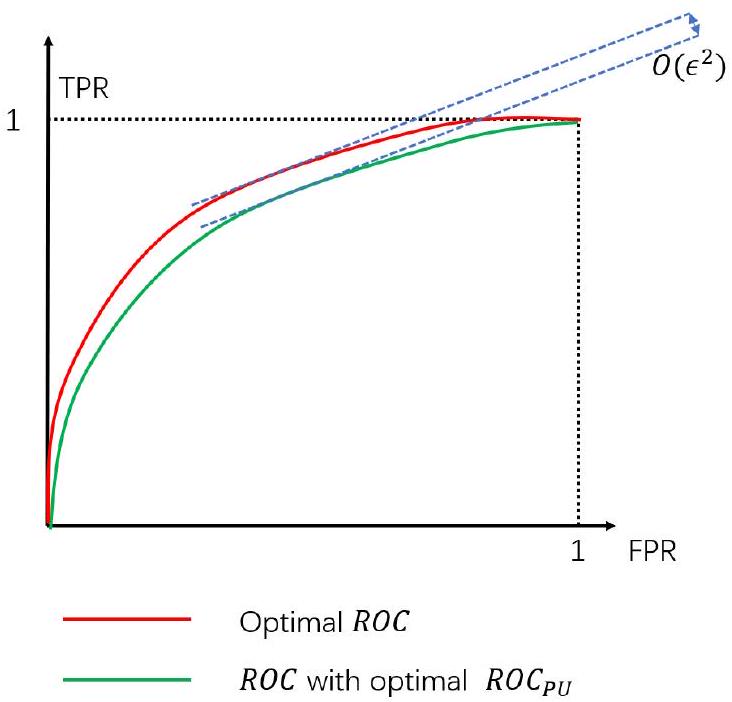
Figure 1: Illustration of the error of the ROC curve obtained by optimizing PU metrics.

Figure 1. Comparison with the optimal $ROC$ with known true label (red curve), versus the $ROC$ when $ROC_{SPU}$ is optimal (green curve). The result indicates that the fluctuation of the conditional expectation of soft label will only cause $O\left(\epsilon^{2}\right)$ deviation of $ROC$, in which $\epsilon$ is the bound in the right hand side of (24).

Now we summarize our findings. We have analyzed the performance of $TPR_{SPU},FPR_{SPU}$ and $AUC_{SPU}$ under three assumptions, in which the first one is the strongest and the last one is the weakest. If Generalized SCAR assumption is satisfied, then these PU metrics can perfectly replace real metrics $TPR,FPR$ and $AUC$, since every improvement on PU metrics implies the improvement on real metrics. If the assumption is weakened, such that we only require $\mathbb{E}[S\mid X]$ to grow monotonically with $\mathbb{E}[Y\mid X]$, then the improvement on PU metrics does not necessarily implies the improvement on real metrics. However, if PU metrics are optimal, then real metrics are also optimal. Then we further weakened the assumption, such that $\mathbb{E}[S\mid X]$ is not required to grow completely monotonic with $\mathbb{E}[Y\mid X]$, a noise with level $\epsilon$ is allowed. In this case, the optimality of PU metrics does not imply the optimality of real metrics, but the gap is only second order small. Therefore, we claim that the PU metrics can, in general, provide us with correct direction to help us design and improve our model.

5 Learning Methods

In section 4, we have shown that after trying to improve these substitute metrics, the distance between our final classifier and the ideal classifier is only $O\left(\epsilon^{2}\right)$. As a result, we can just focus on improving these PU metrics. In this section, we discuss how to optimize these metrics given a real dataset.

To begin with, we assume that we have infinite amount of data. This implies that $\mathbb{E}[S\mid X=x]$ is known for every $x$. In this case, we show the following theorem

Theorem 5.

The $TPR_{SPU}$ and $FPR_{SPU}$ of classifier

$$g^{*}(X)=I(\mathbb{E}[S\mid X]>T)$$ (31)

is on the optimal $ROC_{SPU}$ curve.

This theorem tells us that if the sample size is infinite, such that $\mathbb{E}[S\mid X]$ can be accurately estimated, we can just classify a new sample by checking whether the conditional expectation of soft label is larger than a threshold. Of course, in reality, the amount of data is limited. In this case, we can design a method to approximate $g^{*}(X)$ as close as possible. With this intuition, we propose our method as following: Given a parametric model $g_{s}(x,w)$, e.g. a deep neural network, we minimize the following empirical loss:

$$L_{emp}(w)=-\frac{1}{N}\sum_{i=1}^{N}\left[s_{i}\ln g_{s}\left(x_{i},w\right)+\left(1-s_{i}\right)\ln\left(1-g_{s}\left(x_{i},w\right)\right)\right]$$ (32)

Let $w_{emp}^{*}$ be the minimizer of $L_{emp}(w)$. Now we briefly show that $g\left(x,w_{emp}^{*}\right)$ will converge to the optimal classifier with the growth of sample size $N$ and the model complexity. Define

$$L(w)=-\mathbb{E}\left[S\ln g_{s}(X,w)+(1-S)\ln\left(1-g_{s}(X,w)\right)\right]$$ (33)

and

$$w^{*}=\arg\min L(w).$$ (34)

Then previous research on the convergence of neural network  (Bruck and Goodman, 1988; Kohler and Langer, 2019, 2021; Müller et al., 2012) still hold here, and it can be shown that with the growth of the sample size $N$,

$$\lim_{N\rightarrow\infty}\sup_{x}\left|g_{s}\left(x,w_{emp}^{*}\right)-g_{s}\left(x,w^{*}\right)\right|=0.$$ (35)

Moreover, it can be easily shown from (31) that given the joint distribution of $S$ and $X,L(w)$ is minimized if $g(X,w)=\mathbb{E}[S\mid X]$. From universal approximation theorem, with the growth of complexity, $g_{s}\left(x,w^{*}\right)$ will gradually be closer to $\mathbb{E}[S\mid X]$. Combine this fact with (33), we know that the output score of the model trained by minimizing (30) converges to $\mathbb{E}[S\mid X]$. From Theorem 5, we know that the $TPR_{SPU},FPR_{SPU}$ of the final classifier with thresholding will converge to a point on the optimal $ROC_{SPU}$ curve. Note that it is also possible to use nonparametric classifiers, such as $k$ nearest neighbor classifier (Liu et al., 2006; Zhao and Lai, 2021b, a).

The analysis above shows that the classifier obtained by minimizing (30) converges to the optimal classifier under these PU metrics, including $TPR_{SPU},FPR_{SPU}$ and $AUC_{SPU}$. In the next section, we will test the performance of our new method on some real datasets.

6 Experiments

In this section, we show experiments that validate our soft label PU learning method. Our experiments are conducted on three types of datasets. The first one comes from UCI repository. The second type includes two common image datasets, Fashion MNIST and CIFAR-10. For the first and the second type, since we do not assume the knowledge of class prior, we use $AUC$ instead of accuracy as the metric. Finally, we show the experiment result in anti-cheat task in Tencent Game, which is a realistic task.

6.1 Results on UCI repository

We use three datasets: Diabetes (Strack et al., 2014), Adult and Breast Cancer. These datasets are all fully labeled. However, in training datasets, we assume that the labels are not completely known, and only part of positive samples are labeled. The labeling mechanism is determined in the following way. To begin with, we generate a new feature in the training data, whose values follow a uniform distribution in $[0,0.5]$. Then for each training sample, the probability of being labeled equals the value of this new feature.

Our soft label PU learning method is designed as following. The first step is to identify some features from the dataset that are expected to be related to the probability of being positive. Note that these features are selected from common sense instead of being selected from data. Based on these features, we then generate soft labels.

For the Diabetes dataset, the task is to predict the patients that possibly suffer from diabetes. We expect that the people who visited hospital many times or have received many medical treatments are more likely to be positive than ordinary unlabeled samples. Therefore, we assign soft labels based on four features, i.e. number_medications, number_outpatient, number_emergency and number_inpatient. For the Adult dataset, we need to predict whether a person earns over $50\mathrm{\leavevmode\nobreak\ K}$ a year. We expect that people who have some investments are more likely to earn over $50\mathrm{\leavevmode\nobreak\ K}$, thus capital-gain and capital-loss are two features used to generate soft labels. For the breast cancer dataset, we use worst-radius and worsttexture for soft labels. Actually, in all these three datasets, there may exists better alternative methods to generate soft labels based on the opinions from domain experts.

We use two efficient models to train classifiers based on the generated soft labels, i.e. XGBoost  (Chen and Guestrin, 2016) and LightGBM  (Ke et al., 2017) for classification. To avoid overfitting, we remove the features used to generate soft labels before feeding the training data into models.

To show the effectiveness of the soft label PU learning method, we design a contrast method for baseline, in which we just train a classifier using XGBoost and LightGBM with the labeled positive samples being regarded as positive samples, and those unlabeled as negative samples. Another difference with the soft label PU learning method is that in soft label method, the features used to generate soft labels are removed, while in the baseline method, these features are incorporated in model training.

The AUCs are then compared between the soft label PU learning method and the baseline. The results are shown as follows, in which the AUCs are evaluated using test data with true labels.

Table 1. AUC comparison between soft label PU learning method and baseline.

DATA SET	MODEL	RESULT	BASELINE
DIABETES	XGB	0.721	0.694
DIABETES	LGBM	0.728	0.700
ADULT	XGB	0.834	0.829
ADULT	LGBM	0.863	0.833
BREAST CANCER	XGB	0.934	0.885
BREAST CANCER	LGBM	0.910	0.876

The result shows that for all cases, our soft label PU learning methods perform better than simple PU learning baselines, despite that the generation mechanism for soft labels are actually not very carefully designed. A simple explanation is that since the probability of a positive sample to be labeled depends on the new feature we generated, the labeling mechanism does not satisfy SCAR assumption. In this case, there are some samples that are actually positive, but the labeling mechanism makes them hard to be discovered. With our new method, these hidden positive samples can possibly be assigned a soft label, thus their chances of being identified by classifiers can be greatly enhanced.

6.2 Results on image datasets

We then test the performance of soft label PU learning in two well known image datasets, i.e. Fashion-MNIST and CIFAR10. For these two datasets, we generate soft label under Generalized SCAR assumption, i.e. Assumption 2. To be more precise, for each sample with $Y_{i}=1$, we let

$$\mathbb{P}\left(S_{i}=\frac{k}{4}\right)=\frac{1}{5}$$ (36)

for $k=0,\ldots,4$, which means that each real positive example is labeled with $0,0.25,0.5,0.75$ and 1 with equal probabilities. For each sample with $Y_{i}=0$, we let

$$\mathbb{P}\left(S_{i}=\frac{k}{4}\right)=\frac{\pi(4-k)}{5k(1-\pi)}$$ (37)

for $k=0,\ldots,4$, in which $\pi$ is the ratio of positive samples. It can be proved that by the construction (34) and (35), we have

$$\mathbb{P}(Y=1\mid S=s)=s$$ (38)

for $s=0.25,0.5,0.75$. In this setting, the soft label has the meaning of the probability of a sample with unknown label to be positive.

With this setting, we use a simple convolutional neural network to classify images. Since both two datasets have 10 classes, we select some of classes as positive, while the others are regarded as negative samples. We design two baselines. The first baseline regards all samples with soft labels in $(0,1)$ as ordinary unlabeled samples, while the second baseline regards them as positive samples. The AUC results are shown in the following table, in which BLO and BL1 stand for the first and second baselines, respectively.

Table 2. AUC comparison between soft label PU learning method and baseline.

Dataset	Positive class	Result	Baseline 1	Baseline 2
F-MNIST	0	0.980	0.958	0.978
F-MNIST	$0,2,4,6$	0.994	0.983	0.993
CIFAR 10	0	0.930	0.898	0.900
CIFAR 10	$0,1,8,9$	0.951	0.863	0.936

It can be observed that the soft label PU learning shows the best performance for all cases.

6.3 Results on anti-cheat services in Tencent Games

Finally, we evaluate our method on the anti-cheat tasks in Tencent Games, which is a realistic application. Online video games suffer from all kinds of cheating including game-hacking scripts, fake adult credentials and etc, which hurt user experience severely and lead to a tremendous challenge in terms of legal risk prevention. We have already enacted multiple rules to identify these potential cheaters, and then let them to pass security check. After that, these users can be divided into three groups based on the results. The first group admit that they are cheaters, mainly because security checks are randomly assigned in terms of time and majority of cheaters are not capable to pass the sudden check alone. As a result, accounts in first group will suffer from punishment, including time restriction, account bans and etc. The second group of users pass the checking process successfully. They may indeed be innocent, but it is also possible that they have technical methods to pass the checking procedure. The third group of people skip or fail to pass the security check whose account will be forbidden from playing video games unless the security check is passed or expired. Our goal is to train a classifier to identify users that are possibly cheating, based on the previous security check records and other in-game features. The first group can be regarded as reliable positive samples though the number of them is relatively small. For the rest of the groups, we regarded all of them as unlabeled samples, since there is no way for us to know whether they cheated or not for sure. If we conduct PU learning using traditional methods, then the classifiers trained by the data can only identify ’honest cheaters’ instead of covering all possible cheaters. To cope with this problem, we assign soft labels to unlabeled users, on the basis of data obtained from previous check. And we design two methods to calculated soft labels. Details are shown in Appendix A. We then evaluate the performance of soft label PU learning online. To validate the effectiveness of soft labels, we compare the performance of our new method with a baseline method, in which all unlabeled data are simply regarded as negative samples without soft labels. We use the same three-layer neural network as the classifier in both our new method and the baseline method. After that, we ask users with predicted score higher than a certain threshold to pass security check. The performances are evaluated under two metrics: surrender ratio, defined as the ratio of the number of users who admit themselves as cheaters to the total number of security checks assigned, and the ratio of passing the check, defined as the ratio of the number of passed users to the total number of security checks assigned. A higher surrender ratio and lower ratio of successful pass the security check indicate that the method works better. The results are shown in Table 3.

Table 3. Results of soft label PU learning in anti-cheat task in Tencent Games.

Metric	Method1	Method2	Baseline
Surrender ratio	$2.66\%$	$2.20\%$	$1.84\%$
Pass ratio	$19.7\%$	$24.3\%$	$53.3\%$

The result in Table 3 shows that under both metrics, with both methods for soft label generation, the soft label PU learning method is significantly better than the baseline.

7 Discussion

In this section, we mainly discuss two questions. To begin with, we discuss the potential application of the soft label PU learning method. Then we discuss a common alternative of soft label PU learning method, i.e. use soft label as features and still conduct normal PU learning.

7.1 Potential Applications of our proposed soft label PU learning method

The soft label PU learning method can potentially be used in broadly in many scenarios with only positive and unlabeled data. Generally speaking, if the number of observed positive samples is not enough, or the labeling of positive samples is obviously uneven, or the labeling negative samples is not absolutely accurate, even unlabeled, our method proposed can be applied. Specifically, in section 6, we have discussed the application in the cheater recognition task in Tencent Games. It can mitigate the unlabeled problem in ads recommendation when an ad exposed user disabled the ad tracking leading to a convention unknown observation. Also in medical diagnosis, the observed positive samples are patients that are already diagnosed to have a certain disease. Additionally when our method is used, people who have some related symptoms can be assigned with soft labels depending on their severity. For example, in the diagnosis of Alzheimer’s disease  (Jack Jr et al., 2008), patients who suffer from mild cognitive impairment (MCI) may be assigned with soft labels.

7.2 Comparison with using soft label as features

It may be tempting to use soft label as a feature, and still conducts ordinary PU learning. If the observed positive samples are enough and the labeling is even, then using soft label as features may be better. However, in many applications, labeling is not even and available positive sample size may not be enough. In this case, even if the soft label can be used as a strong feature, the performance of the classifier trained by simple PU method may still not be satisfactory. This has been verified in section 6.1, which shows that after we assign soft labels based on some features that are related to the labels, the AUCs are improved compared with the baseline, which uses these features directly in model training.

8 Conclusion

In this paper, we have proposed soft label PU learning, in which apart from labeled positive and ordinary unlabeled data, we have some additional data that are also unlabeled, but are more likely to be positive. In this case, since $TPR$, $FPR,AUC$ are unknown, we have proposed some substitute metrics to evaluate the performance of a classifier. We have shown that under various different assumptions, these metrics can replace the real metrics well. Therefore, model or feature selection can be conducted with the objective of optimizing the PU metrics instead of real metrics. These analysis motivates us to propose a simple parametric learning method to optimize these PU substitute metrics. Finally, we have conducted experiments on both public datasets and task in the anti-cheat service of Tencent Game to validate our proposed method.

This appendix is organized as follows. In Appendix A, we show the experiment details of soft label generation in Tencent Games. The other sections provide proofs of theorems in the paper.

Appendix A Experiment details

A.1 Details of Soft Label Generation in anti-cheat Task of Tencent Game

Figure 2 is a sketch of the procedure of the game-cheater recognition task. In Tencent games, our goal is to find users who cheat the games in different ways and let them pass a security check for verification. If the check is not passed or is refused, various type of punishment will be given to this player account. For this purpose, we collected some user data avoiding private information including their gaming actions, complains from their teammates or opponents, etc. Based on these data, we have enacted multiple rules, which can select users that are potentially cheater. The users who satisfy at least one rule are then required to pass the security check. After that, some users honestly admit or are recognised by the checking procedure that they are actually cheaters. These users’ accounts will suffer from permanent time restriction, and we use them as positive samples. Some users reject or fail to verify themselves. Then a temporary time restriction will be placed. For these users, we assign them soft labels. Other users successfully passed the security check. They are labeled 0, indicating that they are ordinary negative samples and in our cases, they will be regarded as unlabeled data in case of unknown flaw of the checking procedure. Those players can play games freely without any restrictions. Finally, most of users actually do not satisfy any recognition rules or models. As a result, they are not required to pass any check procedures, and they are also regarded as ordinary unlabeled samples. For users who reject or fail to verify themselves, soft labels are generated using the following two methods.

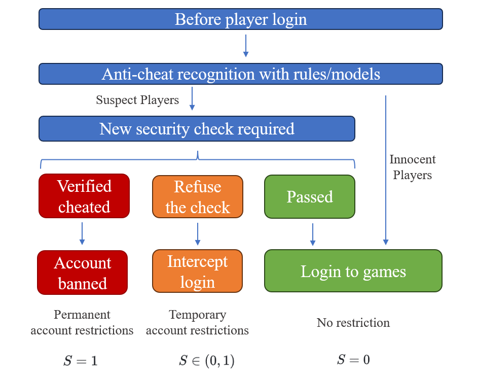
Figure 2: Procedure of game-cheater check and punishment.

A.2 Soft label based on rules

The first method is based on the ratio of users that reject or fail to pass the security check among all users who are required to verify themselves. If such ratio is high, then the rule is likely to be efficient, and the corresponding users are more likely to be cheater. To be more precise, we make the following derivation, in which $R$ denotes a specific rule, $R_{0}$ denotes a special rule which selects users randomly, $F$ denotes the event of rejecting or failing to verify:

$$\mathbb{P}(Y=1|F,R) = \frac{\mathbb{P}(Y=1,F|R)}{\mathbb{P}(F|R)}$$ (39)

$$= \frac{\mathbb{P}(F|R)-\mathbb{P}(Y=0,F|R)}{\mathbb{P}(F|R)}$$

$$\geq 1-\frac{\mathbb{P}(F|Y=0,R)}{\mathbb{P}(F|R)}$$

$$\overset{(a)}{=} 1-\frac{\mathbb{P}(F|Y=0,R_{0})}{\mathbb{P}(F|R)}$$

$$\overset{(b)}{\geq} 1-\frac{\mathbb{P}(F|Y\sim\mathbb{B}{\pi})}{\mathbb{P}(F|R)}$$

$$\approx 1-\frac{\text{Ratio of verification failure under random rule}}{\text{Ratio of verification failure under }R}$$

In (a), we assume that an innocent player rejects or fails to verify himself with equal probabilities for different rules. As a result, the probability of verification failure under each rule equals such probability under a random rule, that is, $P(F|Y=0,R)=P(F|Y=0,R_{0})$. In (b), B denotes Bernoulli distribution, and $\pi=P(Y=1)$ is the positive class prior. We assume that a true cheater are more likely to fail to verify than innocent players.

For every user that rejects or fails security check, the soft label can be assigned as

$$S=1-\frac{\text{Ratio of verification failure under random rule}}{\text{Ratio of verification failure under }R},$$ (40)

then for each soft label $s$,

$$\text{P}(Y=1|S=s)\geq s.$$ (41)

If all soft labels are larger than $\pi$, then Assumption 1 is satisfied. The proof is shown as follows. From Bayes formula,

$$\text{P}(S=s|Y=1)\geq\frac{(1-\pi)s}{\pi(1-s)}\text{P}(S=s|Y=0).$$ (42)

With the condition that $s\notin(0,\pi)$, we have

$$\mathbb{E}[S|Y=1] = \sum_{s}s\mathbb{P}(S=s|Y=1)$$ (43)

$$> \sum_{s}s\mathbb{P}(S=s|Y=0)$$

$$= \mathbb{E}[S|Y=0].$$

Therefore, Assumption 1 is satisfied, and thus the soft label PU learning method can be used here.

A.3 Soft label based on personal security check records

For each user, we collect the security check record within a fixed time period, such as 30 days. Then we let $n_{i}$ be the number of days such that this user is required for security check, and $k_{i}$ be the number of days such that this user passed the security check, $i=1,...,N$,$N$ is the number of all users. The intuition is that if $n_{i}$ is large and $k_{i}$ is small, then the risk of this user to be cheated is high and we need to assign this user a high soft label. The precise rule of soft label is:

$$S_{i}=1-\hat{\theta}_{Bayes,i},$$ (44)

in which $\hat{\theta}_{Bayes,i}$ is the Bayes estimation of the probability such that a user successfully verify himself as an innocent player, which is expressed as

$$\hat{\theta}_{Bayes,i} = \int\theta f(\theta|k_{i})d\theta$$ (45)

$$= \frac{\int\theta f(\theta)\mathbb{P}(k_{i}|\theta)d\theta}{\int f(\theta)\mathbb{P}(k_{i}|\theta)d\theta}$$

$$= \frac{\int f(\theta)\theta^{k_{i}+1}(1-\theta)^{n_{i}-k_{i}}d\theta}{\int f(\theta)\theta^{k_{i}}(1-\theta)^{n_{i}-k_{i}}d\theta}.$$

In the last step, we simply assume that a user passes security check independently with same probabilit, thus $k_{i}$ follows Binomial distribution with parameter $(n_{i},\theta)$.

Now it remains to determine the prior distribution $f(\theta)$. We estimate the prior distribution from data. In particular, we define the log likelihood as

$$L(\theta)=-\frac{1}{N}\sum_{i=1}^{N}\ln\int\binom{n_{i}}{k_{i}}\theta^{k_{i}}(1-\theta)^{n_{i}-k_{i}}f(\theta)d\theta.$$ (46)

Now we get $f(\theta)$ by solving the following optimization problem.

$$\begin{array}[]{cc}\underset{f}{\text{minimize}}&L(\theta)+\lambda\int f^{2}(\theta)d\theta\\ \text{subject to}&\int f(\theta)d\theta=1,f(\theta)\geq 0.\end{array}$$ (49)

$\lambda\int f^{2}(\theta)d\theta$ is a regularization term that prevents overfitting. The optimization is constrained on a probability simplex, hence we can solve it using exponentiated gradient method Beck and Teboulle (2003).

Appendix B Proof of Theorem 1

For simplicity, we only provide the proof assuming that $S$ follows a continuous distribution. If the distribution of $S$ have some mass at some $s$, then we can construct a series of continuous distributions that converges to the true distribution of $S$. Let $f_{S},F_{S}$ be the pdf and cdf of $S$, respectively.

From (3) and (4),

$$TPR_{SPU}=\frac{\mathbb{P}(\hat{Y}=1)}{\mathbb{E}[S]}-\frac{\mathbb{E}[1-S]}{\mathbb{E}[S]}FPR_{SPU}$$ (50)

therefore

$$AUC_{SPU} = \frac{1}{\mathbb{E}[S]}\int_{0}^{1}\mathbb{P}(\hat{Y}=1)dFPR_{SPU}$$ (51)

$$-\frac{\mathbb{E}[1-S]}{\mathbb{E}[S]}\int_{0}^{1}FPR_{SPU}dFPR_{SPU}$$

$$= \frac{1}{\mathbb{E}[S]}-\frac{\mathbb{E}[1-S]}{2\mathbb{E}[S]}-\frac{1}{\mathbb{E}[S]}\int_{0}^{1}FPR_{SPU}d\mathbb{P}(\hat{Y}=1)$$

$$= \frac{1}{2}+\frac{1}{2\mathbb{E}[S]}-\frac{1}{2\mathbb{E}[S]\mathbb{E}[1-S]}$$

$$+\frac{1}{\mathbb{E}[S]\mathbb{E}[1-S]}\int_{0}^{1}\mathbb{E}[S\hat{Y}]d\mathbb{P}(\hat{Y}=1).$$

Define $T$ implicitly, such that $\mathbb{P}(S>T)=\mathbb{P}(\hat{Y}=1)$, then

$$\mathbb{E}[S\hat{Y}] = \mathbb{E}[S\mathbb{P}(\hat{Y}=1\mid S)]$$ (52)

$$= \mathbb{E}[SI(S>T)]+\mathbb{E}[S(\mathbb{P}(\hat{Y}=1\mid S)-I(S>T))]$$

$$\overset{(a)}{=} \mathbb{E}[SI(S>T)]+\mathbb{E}[(S-T)(\mathbb{P}(\hat{Y}=1\mid S)-I(S>T))]$$

$$\overset{(b)}{\leq} \mathbb{E}[SI(S>T)].$$

(a) holds because $\mathbb{E}[\mathbb{P}(\hat{Y}=1|S)-I(S>T)]=\mathbb{P}(\hat{Y}=1)-\mathbb{P}(S>T)=0$. (b) holds because $(S-T)(\mathbb{P}(\hat{Y}=1\mid S)-I(S>T))\leq 0$ always holds.

Therefore

$$\int_{0}^{1}\mathbb{E}[S\hat{Y}]d\mathbb{P}(\hat{Y}=1) \leq \int_{0}^{1}\mathbb{E}[SI(S>T)]d\mathbb{P}(S>T)$$ (53)

$$= \frac{1}{2}-\frac{1}{2}\int_{0}^{1}F_{S}^{2}(u)du.$$

Combine (51) and (53), (11) can be easily derived. The proof is complete.

Appendix C Proof of Theorem 2

For simplicity, we only prove (17) and (19). The proof of (18) is omitted since it is very similar to the proof of (17). From Assumption 3, we have $\mathbb{E}[S\mid Y,\hat{Y}]=\mathbb{E}[S\mid Y]$ since $\hat{Y}$ is a function of $X$. Therefore

$$\mathbb{E}[S\hat{Y}] = \mathbb{E}[SY\hat{Y}]+\mathbb{E}[S(1-Y)\hat{Y}]$$ (54)

$$= \mathbb{E}[Y\hat{Y}]S_{P}+\mathbb{E}[(1-Y)\hat{Y}]S_{N}$$

$$= \pi S_{P}TPR+(1-\pi)S_{N}FPR$$

Moreover,

$$\mathbb{E}[S]=\pi S_{P}+(1-\pi)S_{N},$$ (55)

hence

$$TPR_{SPU}=aTPR+bFPR.$$ (56)

(14) is proved. (15) can be proved in a similar way, thus we omit it. For (16), we have

$$AUC_{SPU} = \int TPR_{SPU}dFPR_{SPU}$$ (57)

$$= ac\int TPRdTPR+bd\int FPRdFPR+ad\int TPRdFPR+bc\int FPRdTPR$$

$$= \frac{1}{2}ac+\frac{1}{2}bd+bc+(ad-bc)AUC$$

$$= \frac{1}{2}(b+c)+(ad-bc)AUC,$$

in which the last step can be simply proved using the expressions from (20) to (23). Furthermore, it is obvious that if $S_{P}>S_{N}$, then $ad-bc>0$.

Appendix D Proof of Theorem 3

Let $\hat{Y}:\mathbb{R}^{d}\rightarrow\{0,1\}$ be a classifier, which is a function of $x$. Define $\eta_{S}(x)=\mathbb{E}[S\mid x]$. We first show the following lemma:

Lemma 1.

Given $\mathbb{P}(\hat{Y}=1)$, if $\hat{Y}=I\left(\eta_{S}(X)>T_{S}\right)$, then $TPR_{SPU}$ is maximized, and $FPR_{SPU}$ is minimized, in which $T_{S}$ is selected such that $\mathbb{P}(\hat{Y}=1)=\mathbb{P}\left(S>T_{S}\right)$.

Proof 

$$\mathbb{E}[S\hat{Y}] = \mathbb{E}\left[\eta_{S}(X)\hat{Y}\right]$$ (58)

$$= \mathbb{E}\left[\eta_{S}(X)I\left(\eta_{S}(X)>T_{S}\right)\right]+\mathbb{E}\left[\eta_{S}(X)\left(\hat{Y}-I\left(\eta_{S}(X)>T_{S}\right)\right)\right]$$

$$\leq \mathbb{E}\left[\eta(X)I\left(\eta_{S}(X)>T_{S}\right)\right].$$

In the last step, equality holds when $\hat{Y}=I\left(\eta_{S}(X)-T_{S}\right)$. From the definition of $TPR_{SPU}$ and $FPR_{SPU}$ in (6) and (7), we know that with $\hat{Y}=I\left(\eta_{S}(X)-T_{S}\right),TPR_{SPU}$ is maximized, and $FPR_{SPU}$ is minimized.  

Therefore, if $g_{S}^{*}$ attains optimal $ROC_{SPU}$, then $g_{S}^{*}$ should be monotonically increasing with $\eta_{S}(x)$. From Assumption 3, $g_{S}^{*}$ is also monotonically increasing with $\eta(\mathbf{x})$. Similar to Lemma 1, it can be proved that $\hat{Y}=I\left(\eta(X)>T_{Y}\right)$ both maximizes $TPR$ and minimizes $FPR$, in which $\eta(X)=$ $\mathbb{E}[Y\mid X]$. Therefore, $g_{S}^{*}$ also attains optimal $ROC$.

Appendix E Proof of Theorem 4

From the proof of Theorem 3, we know that $g^{*}(x)=\eta(x)$ attains optimal $ROC$, while $g_{S}^{*}(x)=\eta_{S}^{*}(x)$ attains optimal $ROC_{SPU}$. For each threshold $T_{Y}\in[0,1]$, define $TPR\left(g,T_{Y}\right)$ as the $TPR$ of classifier $\hat{Y}=I\left(\eta(x)>T_{Y}\right)$, and select $T_{S}$ such that

$$\int_{\eta_{S}(x)\geq T_{S}}f(x)dx=\int_{\eta(x)\geq T_{Y}}f(x)dx.$$ (59)

Then define $TPR\left(g_{S},T_{S}\right)$ as the $TPR$ value of classifier $\hat{Y}=I\left(\eta_{S}(x)>T_{S}\right)$. Then

$$TPR\left(g_{S},T_{S}\right) =\frac{\mathbb{E}\left[YI\left(g_{S}(X)>T_{S}\right)\right]}{\mathbb{E}[Y]}$$ (60)

$$=\frac{1}{\pi}\int_{g_{S}(x)>T_{S}}\eta(x)f(x)dx$$

$$TPR\left(g,T_{Y}\right)= \frac{1}{\pi}\int_{g(X)>T_{Y}}\eta(x)f(x)dx$$

Define

$$A :=\left\{x\mid\eta(x)>T_{Y}\right\}$$ (61)

$$A_{S} :=\left\{x\mid\eta_{S}(x)>T_{S}\right\}$$

Now we bound the difference of the $TPR$ of classifier $I\left(\eta(x)>T_{Y}\right)$ and $I\left(\eta_{S}(x)>T_{S}\right)$ :

$$TPR\left(g,T_{Y}\right)-TPR\left(g_{S},T_{S}\right)$$ (62)

$$= \frac{1}{\pi}\left[\int_{A\setminus A_{S}}\eta(x)f(x)dx-\int_{A_{S}\setminus A}\eta(x)f(x)dx\right]$$

$$= \frac{1}{\pi}\left[\int_{A\setminus A_{S}}\left(\eta(x)-T_{Y}\right)f(x)dx-\int_{A_{S}\setminus A}\left(T_{Y}-\eta(x)\right)f(x)dx\right]$$

$$\leq \frac{1}{\pi C_{h}}\left[\int_{A\setminus A_{S}}\left(h(\eta(x))-h\left(T_{Y}\right)\right)f(x)dx-\int_{A_{S}\setminus A}\left(h\left(T_{Y}\right)-h(\eta(x))\right)f(x)dx\right]$$

$$= \frac{1}{\pi C_{h}}\left[\int_{A\setminus A_{S}}h(\eta(x))f(x)dx-\int_{A_{S}\setminus A}h(\eta(x))f(x)dx\right]$$

$$\leq \frac{1}{\pi C_{h}}\left[\int_{A\setminus A_{S}}\left(h(\eta(x))-\eta_{S}(x)\right)f(x)dx-\int_{A_{S}\setminus A}\left(h(\eta(x))-\eta_{S}(x)\right)f(x)dx\right]$$

$$\leq \frac{2\epsilon}{\pi C_{h}}\int_{A\setminus A_{S}}f(x)dx,$$

in which the last step comes from Assumption 4. For $x\in$ $A\setminus A_{S},\eta_{S}(x)\leq T_{S}$, then from Assumption 4,

$$h(\eta(x))\leq\eta_{S}(x)+\epsilon\leq T_{S}+\epsilon$$ (63)

Moreover, for $x\in A_{S}\setminus A,\eta(x)\leq T_{Y}$, we have

$$T_{S}\leq\eta_{S}(x)\leq h(\eta(x))+\epsilon\leq h\left(T_{Y}\right)+\epsilon$$ (64)

thus $h(\eta(x))\leq h\left(T_{Y}\right)+2\epsilon$, and $\eta(x)-T_{Y}\leq 2\epsilon/C_{h}$. Hence

$$TPR\left(g,T_{Y}\right)-TPR\left(g_{S},T_{S}\right) \leq \frac{2\epsilon}{\pi C_{h}}\int_{\eta(x)\in\left[T_{Y},T_{Y}+2\epsilon/C_{h}\right]}f(x)dx$$ (65)

$$\leq \frac{4M}{\pi C_{h}^{2}}\epsilon^{2},$$

in which the last step comes from (27). Similarly, it can be proved that

$$FPR\left(g_{S},T_{S}\right)-FPR\left(g,T_{Y}\right)\leq\frac{4M}{\pi C_{h}^{2}}\epsilon^{2}.$$ (66)

From (65) and (66), it can be shown that

$$AUC\left(g_{S}^{*}\right)\geq AUC\left(g^{*}\right)-\frac{8M}{\pi C_{h}^{2}}\epsilon^{2}.$$ (67)

Appendix F Proof of Theorem 5

Theorem 5 has been proved in Lemma 1.

References

- Beck and Teboulle (2003) Amir Beck and Marc Teboulle. Mirror descent and nonlinear projected subgradient methods for convex optimization. Operations Research Letters, 31(3):167–175, 2003.
- Bekker and Davis (2018) Jessa Bekker and Jesse Davis. Estimating the class prior in positive and unlabeled data through decision tree induction. In Proceedings of the AAAI conference on artificial intelligence, volume 32, 2018.
- Bekker and Davis (2020) Jessa Bekker and Jesse Davis. Learning from positive and unlabeled data: A survey. Machine Learning, 109:719–760, 2020.
- Bekker et al. (2019) Jessa Bekker, Pieter Robberechts, and Jesse Davis. Beyond the selected completely at random assumption for learning from positive and unlabeled data. In Joint European conference on machine learning and knowledge discovery in databases, pages 71–85. Springer, 2019.
- Bruck and Goodman (1988) Jehoshua Bruck and Joseph W Goodman. A generalized convergence theorem for neural networks. IEEE Transactions on Information Theory, 34(5):1089–1092, 1988.
- Chen et al. (2020a) Hui Chen, Fangqing Liu, Yin Wang, Liyue Zhao, and Hao Wu. A variational approach for learning from positive and unlabeled data. Advances in Neural Information Processing Systems, 33:14844–14854, 2020a.
- Chen and Guestrin (2016) Tianqi Chen and Carlos Guestrin. Xgboost: A scalable tree boosting system. In Proceedings of the 22nd acm sigkdd international conference on knowledge discovery and data mining, pages 785–794, 2016.
- Chen et al. (2020b) Xuxi Chen, Wuyang Chen, Tianlong Chen, Ye Yuan, Chen Gong, Kewei Chen, and Zhangyang Wang. Self-pu: Self boosted and calibrated positive-unlabeled training. In International Conference on Machine Learning, pages 1510–1519. PMLR, 2020b.
- Christoffel et al. (2016) Marthinus Christoffel, Gang Niu, and Masashi Sugiyama. Class-prior estimation for learning from positive and unlabeled data. In Asian Conference on Machine Learning, pages 221–236. PMLR, 2016.
- Du Plessis et al. (2014) Marthinus C Du Plessis, Gang Niu, and Masashi Sugiyama. Analysis of learning from positive and unlabeled data. Advances in neural information processing systems, 27, 2014.
- Du Plessis and Sugiyama (2014) Marthinus Christoffel Du Plessis and Masashi Sugiyama. Class prior estimation from positive and unlabeled data. IEICE TRANSACTIONS on Information and Systems, 97(5):1358–1362, 2014.
- Elkan and Noto (2008) Charles Elkan and Keith Noto. Learning classifiers from only positive and unlabeled data. In Proceedings of the 14th ACM SIGKDD international conference on Knowledge discovery and data mining, pages 213–220, 2008.
- He et al. (2018) Fengxiang He, Tongliang Liu, Geoffrey I Webb, and Dacheng Tao. Instance-dependent pu learning by bayesian optimal relabeling. arXiv preprint arXiv:1808.02180, 2018.
- Hou et al. (2017) Ming Hou, Brahim Chaib-Draa, Chao Li, and Qibin Zhao. Generative adversarial positive-unlabelled learning. arXiv preprint arXiv:1711.08054, 2017.
- Jack Jr et al. (2008) Clifford R Jack Jr, Matt A Bernstein, Nick C Fox, Paul Thompson, Gene Alexander, Danielle Harvey, Bret Borowski, Paula J Britson, Jennifer L. Whitwell, Chadwick Ward, et al. The alzheimer’s disease neuroimaging initiative (adni): Mri methods. Journal of Magnetic Resonance Imaging: An Official Journal of the International Society for Magnetic Resonance in Medicine, 27(4):685–691, 2008.
- Ke et al. (2017) Guolin Ke, Qi Meng, Thomas Finley, Taifeng Wang, Wei Chen, Weidong Ma, Qiwei Ye, and Tie-Yan Liu. Lightgbm: A highly efficient gradient boosting decision tree. Advances in neural information processing systems, 30, 2017.
- Kiryo et al. (2017) Ryuichi Kiryo, Gang Niu, Marthinus C Du Plessis, and Masashi Sugiyama. Positive-unlabeled learning with non-negative risk estimator. Advances in neural information processing systems, 30, 2017.
- Kohler and Langer (2019) Michael Kohler and Sophie Langer. On the rate of convergence of fully connected very deep neural network regression estimates. arXiv preprint arXiv:1908.11133, 2019.
- Kohler and Langer (2021) Michael Kohler and Sophie Langer. On the rate of convergence of fully connected deep neural network regression estimates. The Annals of Statistics, 49(4):2231–2249, 2021.
- Liu et al. (2006) Ting Liu, Andrew W Moore, Alexander Gray, and Claire Cardie. New algorithms for efficient high-dimensional nonparametric classification. Journal of Machine Learning Research, 7(6), 2006.
- Müller et al. (2012) Berndt Müller, Joachim Reinhardt, and Michael T Strickland. Neural networks: an introduction. Springer Science & Business Media, 2012.
- Northcutt et al. (2017) Curtis G Northcutt, Tailin Wu, and Isaac L Chuang. Learning with confident examples: Rank pruning for robust classification with noisy labels. arXiv preprint arXiv:1705.01936, 2017.
- Strack et al. (2014) Beata Strack, Jonathan P DeShazo, Chris Gennings, Juan L Olmo, Sebastian Ventura, Krzysztof J Cios, John N Clore, et al. Impact of hba1c measurement on hospital readmission rates: analysis of 70,000 clinical database patient records. BioMed research international, 2014, 2014.
- Zhao and Lai (2021a) Puning Zhao and Lifeng Lai. Efficient classification with adaptive knn. In Proceedings of the AAAI Conference on Artificial Intelligence, volume 35, pages 11007–11014, 2021a.
- Zhao and Lai (2021b) Puning Zhao and Lifeng Lai. Minimax rate optimal adaptive nearest neighbor classification and regression. IEEE Transactions on Information Theory, 67(5):3155–3182, 2021b.