Graph Neural Network based Active and Passive Beamforming for Distributed STAR-RIS-Assisted Multi-User MISO Systems

Abstract

This paper investigates a joint active and passive beamforming design for distributed simultaneous transmitting and reflecting (STAR) reconfigurable intelligent surface (RIS) assisted multi-user (MU)- mutiple input single output (MISO) systems, where the energy splitting (ES) mode is considered for the STAR-RIS. We aim to design the active beamforming vectors at the base station (BS) and the passive beamforming at the STAR-RIS to maximize the user sum rate under transmitting power constraints. The formulated problem is non-convex and nontrivial to obtain the global optimum due to the coupling between active beamforming vectors and STAR-RIS phase shifts. To efficiently solve the problem, we propose a novel graph neural network (GNN)-based framework. Specifically, we first model the interactions among users and network entities are using a heterogeneous graph representation. A heterogeneous graph neural network (HGNN) implementation is then introduced to directly optimizes beamforming vectors and STAR-RIS coefficients with the system objective. Numerical results show that the proposed approach yields efficient performance compared to the previous benchmarks. Furthermore, the proposed GNN is scalable with various system configurations.

I Introduction

Beyond fifth-generation (B5G) and sixth-generation (6G) wireless communication networks are expected to cope with the explosive increase in the number of wireless devices with a focus on spectral and energy efficiency[1]. In this light, RISs have emerged as a promising technology capable of significantly enhancing the sum rate and energy efficiency of wireless networks.[2]. An RIS is a flat meta-surface containing a number of inexpensive passive reflecting components, which can be adjusted through a controller to smartly manage the propagation of the incident signals with low power consumption. Moreover, RIS deployment allows for the establishment of a connection between the BS and user equipment (UE), especially in scenarios where they are situated in areas with no service or where direct links are obstructed. Nevertheless, typical RISs are only capable of reflecting incident signals, hence only users located in the $180^{o}$ half-plane can be supported by the RISs. Consequently, the positioning of both the BS and users is constrained to be on the same side as the RISs, which restricts their deployment. As a remedy, the STAR-RIS emerges as a promising technology that overcomes the constraints of conventional RIS setups as it can extend the coverage from half-space to a complete $360^{o}$ space[3]. Specifically, the STAR-RIS divides the three-dimensional (3D) space into two distinct regions, i.e., the transmission region ($\mathcal{T}$ region) and the reflection region ($\mathcal{R}$ region). Therefore, compared to conventional RISs, STAR-RISs can provide new degrees-of-freedom (DoFs) that enhance the system performance [3].

Due to its significant potential, researchers in both industry and academia have directed considerable attention toward STAR-RIS and its variations. Many works have exploited the STAR-RIS in various system settings. In [3], the authors examined a MISO system aided by STAR-RIS, and focused on a problem aimed at minimizing power consumption while considering active and passive beamforming. Furthermore, STAR-RISs were employed in non-orthogonal multiple access (NOMA) systems to enhance the performance gain. In [4], the authors delved into a problem of optimizing both active beamforming vectors and STAR-RIS phase shifts to enhance the energy efficiency and overall sum rate of NOMA systems. An iteration based semidefinite relaxation (SDR) scheme was proposed to tackle the non-convexity. In [5], the authors examined the coverage characterization of a two-user system aided by STAR-RIS with a joint optimization of power allocation at the access point and the STAR-RIS coefficients. The non-convex decoding order constraint in the problem was re-transformed into a convex one by applying KKT conditions. Nevertheless, most of the current research has focused on single STAR-RIS-assisted wireless systems, while the benefits of deploying multiple intelligent reflecting surfaces have been investigated in [6, 7, 8, 9]. As opposed to the single RIS scenario, the distributed employment has revealed its potential for enhancing coverage, signal power, and system energy efficiency. Therefore, it is crucial to extend the study of STAR-RIS-assisted systems to encompass the distributed scenario.

While STAR-RISs have been extensively explored in the existing literature, traditional designs face challenges due to their high computational complexity. Unlike conventional RIS systems, transmission and reflection elements in STAR-RIS systems are coupled together, which further increase the resource allocation complexity [3]. In this light, deep learning (DL) has stood out as a cost-effective solution for the intelligent reflecting surfaces assisted system optimization [10, 11, 12, 13]. Particularly, fully connected neural networks (FCNNs) were proposed in [10] passive beamforming optimization problem in RIS-assisted single user systems. FCNNs were trained via a unsupervised training procedure to predict the local optimum solution maximizing user’s achievable rate directly from channel information. In addition, an end-to-end design was proposed for a double-RIS aided MIMO system in [11] to optimize the system’s reliability, where each device was represented as a one-dimensional CNN (1D-CNN) model and all the models were jointly trained to reduce the symbol detection error rate. It was proved that the proposed end-to-end design can provide a promising performance with low complexity compared to the conventional optimization approach. DL models have utilities of optimizing STAR-RIS systems. The authors in [12] proposed a deep deterministic policy gradient (DDPG)-based framework to optimize the energy efficiency of STAR-RIS-aided NOMA systems. The transmitting beamforming vectors and STAR-RIS coefficient were jointly optimized based on the CSI via an trial-and-error process. Furthermore, the authors in [13] proposed two solutions for the joint active and passive beamforming optimization in STAR-RIS-aided NOMA systems, namely the hybrid DDPG algorithm and the joint DDPG and deep Q network algorithm. It was shown that the proposed solutions achieve superior performance compared to the conventional DDPG framework, albeit with increased computational complexity.

Despite the commendable performance and low complexity of traditional DL models, they lacked the versatility to generalize across various network sizes, such as differing numbers of users and RIS elements. This limitation stems from the fixed output/input dimensions inherent in these models; thus, an FCNN/CNN trained with a specific configuration cannot be seamlessly applied to others. Consequently, the practical utility of DL models is significantly hampered, especially in dynamic system configurations. One potential remedy entails training multiple DL models tailored to different configurations and switching them accordingly based on real-time system settings. However, this approach is inherently cumbersome due to its demand for prohibitively high training complexity and storage memory.

Given the constraints on the dimensions of traditional FCNN/CNN models, our primary objective is to devise a DL design for distributed STAR-RIS-aided MU-MISO systems that are scalable to different system settings with varying numbers of users and STAR-RIS elements. To accomplish this, the designed deep neural network (DNN) must maintain dimensional invariance in its input processing, irrespective of system configurations. The development of such neural networks has been explored within the framework of (GNNs)[14], initially crafted for managing graph-structured data. In GNN layers, each vertex is meticulously engineered to remain invariant to changes in network dimensions and input sequences. This approach preserves both permutation invariance (PI) and permutation equivariance (PE) within the model, as demonstrated in the previous work [15].

In other words, GNNs are able to learn the underline interaction between network entities and generalize well with the varying number of order of them. Motivated by this property, GNNs have been extended to solve many scalable wireless communication systems [16, 17, 18, 19, 20, 21]. In [16, 17, 18], the homogeneous GNN was utilized to address power management concerns within device-to-device (D2D) wireless networks, where each transmitter-receiver pair is model as a vertex of the graph, and their interfering channels are model as edges. Owing to parameter sharing among vertices, these GNN models demonstrate remarkable generalization across different numbers of transceiver pairs. Furthermore, GNN models have been extended to more intricate wireless networks encompassing devices of diverse types. In [19, 20], heterogeneous GNNs were employed to model MU-MISO systems. This approach involved representing each antenna and user as distinct types of vertices, and the explicit channels between them are exploited as weights of edges in the graph. By facilitating information exchange between vertex types via heterogeneous message passing inference, the devised GNN models adeptly estimated the precoding matrix, yielding notable performance gains compared to conventional beamforming benchmarks.

Motivated by the above challenges and the recent success of GNN, this paper investigates the optimization problem of jointly optimizing active and passive beamforming for distributed STAR-RIS-aided MU-MISO systems. Specifically, we delve into the coordinated optimization of active beamforming vectors at the BS, the STAR-RIS phase shifts, and the STAR-RIS amplitude coefficients. Our objective is to maximize the total user throughput while adhering to predefined power constraints. Within this framework, we introduce a novel Heterogeneous Graph Neural Network (HGNN) approach for the joint optimization of active beamforming vectors at the BS, the STAR-RIS phase shifts, and the STAR-RIS amplitude coefficients. Specifically, we propose an HGNN design where each element of the STAR-RIS and each user are represented as distinct types of vertices within the graph structure. The information between them is then propagated through the entire graph via a heterogeneous message-passing procedure dedicated to the considered problem. The designed HGNN is then trained via an unsupervised fashion to enhance the system sum rate. Our primary contributions are outlined as follows

• We formulate a sum rate optimization problem for distributed STAR-RIS-assisted MU-MISO systems. As the distributed STAR-RIS assisted systems have not been studied in literature, we first present a conventional optimization technique to solve the problem and use it as a benchmark of the proposed HGNN approach. Specifically, the original problem are decomposed into sub-problems corresponding to each variable. Then, an alternation optimization (AO) algorithm based on successive convex approximation (SCA) technique is applied to optimize the problem in an iterative manner.

• We investigate the PE property of the beamforming policy in the considered system and propose a heterogeneous graph representation to model the considered wireless networks. Each STAR-RIS element and user is modeled as a vertex of the graph, and the corresponding equivalent channel is used as edges connecting them. Consequently, we propose a heterogeneous graph message passing (HGMP) algorithm dedicated to beamforming tasks which facilitates the information exchange through the entire graph. We then prove that the PE property is well-preserved in the proposed HGMP.

• We present an effective implementation of the beamforming heterogeneous graph neural network (BHGNN) model executing the proposed message-passing algorithm. Specifically, each function within the HGMP algorithm is approximated by an FCNN model with trainable parameters. The forward propagation of the designed BHGNN model is executed aligned with the HGMP algorithm and the model is then trained to optimize the system sum rate. S. Given that the dimensions of vertices and edges remain unaffected by the system’s configuration, our designed BHGNN demonstrates strong generalization capabilities across various system settings, rendering it suitable for dynamic networks.

• We produce extensive simulations to validate the efficacy of the proposed methodology. The numerical results indicate that the HGNN can attain performance levels close to those of the AO-based approach with much lower computational complexity. Additionally, the HGNN model exhibits robust generalization across varying numbers of users, STAR-RIS elements, and user distributions.

The rest of this paper is organized as follows: Section II introduces the system model and outlines the formulation of the problem aiming to maximize user sum rates. In section III an AO-based solution is presented to address the formulated problem. Section IV introduces a heterogeneous graph representation for the system and proposes a GNN-based solution to jointly optimize beamforming vectors and STAR-RIS phase shifts, maximizing the system sum rate. The numerical results and discussions are detailed in Section V, and Section VI offers the primary conclusions drawn from this paper.

Notation: Matrices are presented by bold capital letters, and lower bold letters denote vectors. The regular transpose and Hermitian transpose of a matrix $\mathbf{A}$ are denoted by $\mathbf{A}^{T}$ and $\mathbf{A}^{H}$, respectively. The trace of a square matrix $\mathbf{A}$ is denoted by $\mathrm{tr}(\mathbf{A})$, while its inverse is represented as $\mathbf{A}^{-1}$. Furthermore, $\mathrm{Re}(.)$ and $\mathrm{Im}(.)$ are employed to represent the real and imaginary parts, respectively, of the given argument. $\|\cdot\|$ represents the Euclidean norm, and $\mathcal{CN}(\cdot,\cdot)$ is a circularly symmetric Gaussian distribution. $\nabla f(\cdot)$ denotes the derivative of function $f(\cdot)$. Finally, $\mathcal{O}(\cdot)$ is the big-$\mathcal{O}$ notation.

II System model and problem formulation

This section describe the distributed STAR-RIS system under study in the paper. We formulate a problem aimed at maximizing the sum rate while adhering to constrained power limits, specifically addressing the joint design of active and passive beamforming.

II-A System model

We investigate a distributed MISO system aided by STAR-RIS, where a BS with $N_{t}$ antennas serves $K$ individual users, each equipped with a single antenna, positioned on either the transmission side $(\mathcal{T})$ or the reflection side $(\mathcal{R})$. To enhance the system spectral efficiency, $L$ STAR-RISs are deployed to support the transmission, each of which contains $M$ elements.

In this paper, we make the assumption that the STAR-RISs operate in the energy splitting (ES) mode, which entails partitioning the power of the incoming signal into transmitted and reflected signal energies. Consequently, the matrices representing the transmission and reflection coefficients of the $l$-th STAR-RIS are expressed as

$$\boldsymbol{\Phi}_{l}^{\chi}=\mathrm{diag}\left(\sqrt{\beta_{l1}^{\chi}}e^{\theta_{l1}^{\chi}},\cdots,\sqrt{\beta_{lM}^{\chi}}e^{\theta_{lM}^{\chi}}\right),$$ (1)

where $\chi\in\{\mathcal{T},\mathcal{R}\}$. For brevity, we represent $\boldsymbol{\beta}_{l}^{\chi}=[\sqrt{\beta_{l1}^{\chi}},\cdots,\sqrt{\beta_{lM}^{\chi}}]^{T}$ and $\mathbf{\Theta}_{l}^{\chi}=[e^{j\theta_{l1}^{\chi}},\cdots,e^{j\theta_{lM}^{\chi}}]^{T}$ as the amplitude and phase shift vectors, respectively, of the $l$-th STAR-RIS in the transmitter and receiver regions. Additionally, this study assumes that direct links between the base station (BS) and users are obstructed by obstacles.

Among the $K$ users, we consider the initial $K_{0}$ users positioned in the $t$ region, while the rest $(K-K_{0})$ users are situated in the $r$ region. Specifically, $\chi=\mathcal{T}$ if $k\in{1,2,\cdots,K_{0}}$, otherwise $\chi=\mathcal{R}$. The received signal at the $k$-th user is expressed as

$$y_{k}=\sum_{l=1}^{L}\mathbf{h}_{kl}^{H}\mathrm{diag}(\boldsymbol{\beta}_{l}^{\chi})\mathrm{diag}(\mathbf{\Theta}_{l}^{\chi})\mathbf{G}_{l}\mathbf{x}+n_{k},$$ (2)

where $\mathbf{x}=\sum_{k=1}^{K}\mathbf{w}_{k}s_{k}$ represents the transmitted symbols, and $n_{k}\sim\mathcal{CN}(0,\sigma^{2})$ denotes additive white Gaussian noise. Moreover, $\mathbf{h}_{kl}\in\mathbb{C}^{M}$ represents the channel from the $l$-th RIS to the $k$-th user, and $\mathbf{G}_{l}\in\mathbb{C}^{M\times N_{t}}$ signifies the channel from the BS to the $l$-th RIS. The signal-to-interference-and-noise ratio (SINR) at the $k$-th user is represented as

$$\gamma_{k}=\frac{\left|\sum_{l=1}^{L}\mathbf{h}_{kl}^{H}\boldsymbol{\Phi}_{l}^{\chi}\mathbf{G}_{l}\mathbf{w}_{k}\right|^{2}}{\sum_{j\in\mathcal{K},j\neq k}\left|\sum_{l=1}^{L}\mathbf{h}_{kl}^{H}\boldsymbol{\Phi}_{l}^{\chi}\mathbf{G}_{l}\mathbf{w}_{j}\right|^{2}+\sigma^{2}},$$ (3)

where $\mathcal{K}=\{1,2,\cdots,K\}$ is the set of user. The SINR expression in (3) reveals that compared to a centralized STAR-RIS system, the distributed RISs gain the potential for increased spatial diversity, enhanced interference mitigation by cooperatively optimizing STAR-RIS phase shifts over multiple channel realizations. Moreover, the potential gain is in the order of $\mathcal{O}(L^{2}M^{2})$ thanks to the coherent signal processing.

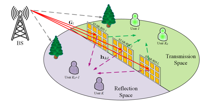
Figure 1: The considered distributed STAR-RIS system model.

II-B Problem Formulation

Our objective is to maximize the system sum rate of all users while adhering to the transmit power constraint by jointly optimizing the precoding vector $\mathbf{w}_{k}$, the STAR-RIS phase shift $\mathbf{\Theta}^{\chi}$, and the amplitude coefficients $\boldsymbol{\beta}_{l}^{\chi}$. Mathematically, the optimization problem is formulated as

$$\underset{\{\mathbf{W},\mathbf{\Theta}^{\chi},\boldsymbol{\beta}^{\chi}\}\textperiodcentered}{\mathrm{maximize}} \sum_{k\in\mathcal{K}}\log_{2}(1+\gamma_{k})$$ (4a)

subject to $$\mathbf{W}^{H}\mathbf{W}\leq P_{\max},$$ (4b)

$$\theta_{lm}^{\chi}\in[0,2\pi],\quad\forall l\in\mathcal{L},m\in\mathcal{M},$$ (4c)

$$0\leq\beta_{lm}^{\chi}\leq 1\quad\forall l\in\mathcal{L},m\in\mathcal{M},$$ (4d)

$$(\beta_{lm}^{T})^{2}+(\beta_{lm}^{R})^{2}\leq 1,\forall l\in\mathcal{L},m\in\mathcal{M},$$ (4e)

where $\mathcal{M}=\{1,2,\cdots,M\}$ is the set of STAR-RIS phase shift elements. Besides, $\mathcal{L}=\{1,2,\cdots,L\}$ is the set for STAR-RISs. The stacked beamforming vector of all $K$ user is $\mathbf{W}=[\mathbf{w}_{1}^{T},\mathbf{w}_{2}^{T},\cdots,\mathbf{w}_{K}^{T}]^{T}\in\mathbb{C}^{N_{t}K}$. Similarly, the stacked phase shift matrix of all the $L$ STAR-RISs is $\mathbf{\Theta}^{\chi}=[(\mathbf{\Theta}_{1}^{\chi})^{T},\cdots(\mathbf{\Theta}_{L}^{\chi})^{T}]^{T}$, $\boldsymbol{\beta}^{\chi}=[(\boldsymbol{\beta}_{1}^{\chi})^{T},\cdots,(\boldsymbol{\beta}_{L}^{\chi})^{T}]^{T}$. In (4), $P_{\mathrm{max}}$ is the transmit power budget at the BS. For the constraints, (4b) represents the total transmit power constraint, and (4c) defines the phase shift constraint for each STAR-RIS element. In addition, (4d) and (4e) denote the constraints on the conservation law of energy at the STAR-RIS. One can prove that the problem (4) is non-convex and NP-hard by exploiting the same methodology as in [22] with the maximal independent set. Apart from this, the coupling of transmit beamforming and STAR-RIS phase shifts makes the problem (4) challenging to obtain a global solution. Consequently, in the next sections, we present two alternative frameworks that obtain feasible solutions for the considered problem, namely an AO-based iterative algorithm and a heterogeneous GNN-based solution.

III AO-based Solution of Joint Beamforming Optimization Problem

This section presents an AO-based solution to jointly optimize beamforming vectors and STAR-RIS elements. Specifically, we decompose the problem (4) into three sub-problems corresponding to separate variables, i.e. $\mathbf{w}_{k}$, $\boldsymbol{\beta}^{\chi}$, and $\mathbf{\Theta}^{\chi}$, and solve each of them in an iterative manner.

III-A Phase shift optimization

For given $\mathbf{w}_{k}$ and $\boldsymbol{\beta}^{\chi}$, the problem (4) can be re-written as

$$\underset{\boldsymbol{\Theta}^{\chi},\boldsymbol{\eta}}{\mathrm{maximize}} \sum_{k\in\mathcal{K}}\log_{2}(1+\eta_{k})$$ (5a)

subject to $$\eta_{k}\leq\frac{\left|\sum_{l=1}^{L}\mathbf{h}_{kl}^{H}\boldsymbol{\Phi}_{l}^{\chi}\mathbf{G}_{l}\mathbf{w}_{k}\right|^{2}}{\sum_{i\in\mathcal{K},i\neq k}\left|\sum_{l=1}^{L}\mathbf{h}_{kl}^{H}\boldsymbol{\Phi}_{l}^{\chi}\mathbf{G}_{l}\mathbf{w}_{i}\right|^{2}+\sigma^{2}}$$

$$\forall k\in\mathcal{K},$$ (5b)

$$\theta_{lm}^{k}\in[0,2\pi],\quad\forall l\in\mathcal{L},m\in\mathcal{M},$$ (5c)

where $\boldsymbol{\eta}=[\eta_{1},\cdots,\eta_{k}]^{T}$ stands for a slack variable, ensuring the constraint (5b) remains satisfied at all times, maintaining equality at the optimal solution. Let us introduce $s_{ln}^{\chi}=e^{j\theta_{ln}^{\chi}}$, then with this, we can show that $\mathbf{h}_{kl}^{H}\mathrm{diag}(\boldsymbol{\beta}_{l}^{\chi})\mathbf{\Theta}_{l}^{\chi}\mathbf{G}_{l}\mathbf{w}_{i}=\mathbf{t}_{kil}^{H}\mathbf{s}_{l}^{\chi}$, where $\mathbf{t}_{kil}=(\mathrm{diag}(\mathbf{h}_{kl}^{H})\mathrm{diag}(\boldsymbol{\beta}_{l}^{\chi})\mathbf{G}_{l}\mathbf{w}_{i})^{\ast}\in\mathbb{C}^{M}$, and $\mathbf{s}_{l}^{\chi}=[s_{l1}^{\chi},\cdots,s_{lM}^{\chi}]$. The constraint (5b) can be recast as

$$\eta_{k}\leq\frac{|\mathbf{t}_{kk}^{H}\mathbf{s}^{\chi}|^{2}}{\sum_{i\in\mathcal{K},i\neq k}|\mathbf{t}_{ki}^{H}\mathbf{s}^{\chi}|^{2}+\sigma^{2}},$$ (6)

where the new vectors are defined as $\mathbf{s}^{\chi}=[s_{11}^{\chi},\cdots,s_{1M}^{\chi},\cdots,s_{LM}^{\chi}]^{T}$, and $\mathbf{t}_{ki}=[\mathbf{t}_{ki1};\cdots;\mathbf{t}_{kiL}]$. Consequently, the problem (5) can be reformulated as

$$\underset{\boldsymbol{\eta},\mathbf{s}\textperiodcentered}{\mathrm{maximize}} \sum_{k\in\mathcal{K}}\log_{2}(1+\eta_{k})$$ (7a)

subject to $$|s_{lm}^{\chi}|=1,\quad\forall l\in\mathcal{L},m\in\mathcal{M},$$ (7b)

$$\eta_{k}\leq\frac{|\mathbf{t}_{kk}^{H}\mathbf{s}^{\chi}|^{2}}{\sum_{i\in\mathcal{K},i\neq k}|\mathbf{t}_{ki}^{H}\mathbf{s}^{\chi}|^{2}+\sigma^{2}},\forall k\in\mathcal{K}.$$ (7c)

The problem (7) is, however, still non-convex due to the presence of the unit modulo constraint and the non-convex nature of constraints (6). We first relax the unit modulo constraint by applying the penalty method and the problem (6) now can be expressed as

$$\underset{\boldsymbol{\eta},\mathbf{s}\textperiodcentered}{\mathrm{maximize}} \sum_{k=1}^{K}\log_{2}(1+\eta_{k})+C\sum_{k=1}^{K}\sum_{l=1}^{L}\sum_{m=1}^{M}(|s_{lm}^{\chi}|^{2}-1),$$ (8a)

subject to $$|s_{lm}^{\chi}|\leq 1,\quad\forall l\in\mathcal{L},m\in\mathcal{M},$$ (8b)

$$\eqref{eq:eta_inequality},$$ (8c)

where $C$ is a large positive constant. Next, the SCA method is applied to handle the non-convex objective and constraints. Specifically, the (8) can be approximated using the first order Taylor approximation as

$$\begin{split}&\sum_{k=1}^{K}\log_{2}(1+\eta_{k})+\\ &2C\sum_{k=1}^{K}\sum_{l=1}^{L}\sum_{m=1}^{M}\mathrm{Re}(((s_{lm}^{\chi})^{(n)})^{H}({s}_{lm}^{\chi}-(s_{lm}^{\chi})^{(n)})))\end{split}$$ (9)

To handle the non-convexity in the constraints (6), we introduce a slack variable $\alpha_{k}$ and decompose each constraint of (6) into two following constraints

$$|\mathbf{t}_{kk}^{H}\mathbf{s}^{\chi}|^{2}\geq\alpha_{k}\eta_{k},$$ (10)

$$\sum_{i\in\mathcal{K},i\neq k}|\mathbf{t}_{ki}^{H}\mathbf{s}^{\chi}|^{2}+\sigma^{2}\leq\alpha_{k},$$ (11)

where (11) is already convex as aligned with the second-order cone. To address the non-convex nature of (10), we first rewrite the constraint (10) as

$$-|\mathbf{t}_{kk}^{H}\mathbf{s}^{\chi}|^{2}+\frac{1}{4}(\alpha_{k}+\eta_{n})^{2}-\frac{1}{4}(\alpha_{k}-\eta_{k})^{2}\leq 0.$$ (12)

Since the first and third term of (12) are concave, we employ the Taylor approximation as

$$\begin{split}&-|\mathbf{t}_{kk}^{H}\mathbf{s}^{\chi}|^{2}+\frac{1}{4}(\alpha_{k}+\eta_{n})^{2}-\frac{1}{4}(\alpha_{k}-\eta_{k})^{2}\leq\frac{1}{4}(\alpha_{k}+\eta_{n})^{2}\\ &-2\mathrm{Re}((\mathbf{t}_{kk}^{H}(\mathbf{s}^{\chi})^{(n)})^{H}\mathbf{t}_{kk}^{H}(\mathbf{s}^{\chi}-(\mathbf{s}^{\chi})^{(n)}))-|\mathbf{t}_{kk}^{H}(\mathbf{s}^{\chi})^{(n)}|^{2}\\ &-\frac{1}{4}(2(\alpha^{(n)}_{k}-\eta_{k}^{(n)})(\alpha_{k}-\eta_{k})-(\alpha^{(n)}_{k}-\eta_{k}^{(n)})^{2}).\end{split}$$ (13)

Thus, constraint (12) around $(\mathbf{s}^{\chi})^{(n)}$ and $\eta_{k}^{(n)}$ and can be locally approximated as

$$\begin{split}&-2\mathrm{Re}((\mathbf{t}_{kk}^{H}(\mathbf{s}^{\chi})^{(n)})^{H}\mathbf{t}_{kk}^{H}(\mathbf{s}^{\chi}-(\mathbf{s}^{\chi})^{(n)}))-|\mathbf{t}_{kk}^{H}(\mathbf{s}^{\chi})^{(n)}|^{2}\\ &+\frac{1}{4}((\alpha_{k}+\eta_{n})^{2}-2(\alpha^{(n)}_{k}-\eta_{k}^{(n)})(\alpha_{k}-\eta_{k})\\ &+(\alpha^{(n)}_{k}-\eta_{k}^{(n)})^{2})\leq 0.\end{split}$$ (14)

Note that although a Taylor series approximated function does not ensure the original inequality in general, the inequality locally holds around the tangent point.

Then, the problem (5) can be recast into the following approximated convex problem:

$$\underset{\mathbf{s},\eta,\alpha\textperiodcentered}{\mathrm{maximize}} \sum_{k\in\mathcal{K}}\log_{2}(1+\eta_{k})+$$ (15a)

$$2C\sum_{k=1}^{K}\sum_{l=1}^{L}\sum_{m=1}^{M}\mathrm{Re}(((s_{lm}^{\chi})^{(n)})^{H}({s}_{lm}^{\chi}-(s_{lm}^{\chi})^{(n)})))$$

subject to $$\alpha_{k}\geq 0,\quad\forall k\in\mathcal{K},$$ (15b)

$$|s_{lm}^{\chi}|\leq 1,\quad\forall l\in\mathcal{L},m\in\mathcal{M},$$ (15c)

$$\eqref{eq:inequa2},\eqref{eq:inequa1Taylor},\quad\forall k\in\mathcal{K}.$$ (15d)

The problem (5) can be addressed by repeatedly solving the approximated convex problem (15), employing the SCA method. The details of the SCA algorithm for solving (5) is summarized in Algorithm 1. We directly follow [23, Proposition 3] to provide a lemma that guarantees the convergence of Algorithm 1 as follow.

Lemma 1.

The objective value in (8) achieved by Algorithm 1 is monotonically increasing and the variables $({\mathbf{s}}^{\chi})^{(n)}$, ${\alpha}_{k}^{(n)}$, ${\eta}_{k}^{(n)}$ converge to the points that fulfill the KKT of the problem (8).

Lemma 1 demonstrates that by iteratively solving the approximate problem (15), we can conduct a series of feasible solutions that eventually converge to the KKT solution of the problem (8). With a proper penalty factor $C$, we can find a feasible solution for the original problem (5) by following Algorithm 1.

Algorithm 1 SCA for solving the problem (5)

1:Initialization: $(\mathbf{s}^{\chi})^{(0)},\alpha_{k}^{(0)},\eta_{k}^{(0)},k\in\{1,2\}$ and the iteration index $n=0$.

2:repeat

3: Solve the convex problem (15) to obtain $(\hat{\mathbf{s}}^{\chi})^{(n)},\hat{\alpha}_{k}^{(n)},\hat{\eta}_{k}^{(n)},k\in\mathcal{K}$.

4: Update:

5:  $(\mathbf{s}^{\chi})^{(n+1)}=(\hat{\mathbf{s}}^{\chi})^{(n)}$.

6:  $\alpha_{k}^{(n+1)}=\hat{\alpha}_{k}^{(n)}$

7:  $\eta_{k}^{(n+1)}=\hat{\eta}_{k}^{(n)}$

8:  $t:=t+1$.

9:until The fractional increment in the objective function in (5) remains below a specified threshold $\epsilon_{1}>0$.

10:Return $\mathbf{s}^{\chi*}=(\hat{\mathbf{s}}^{\chi})^{(n)},\alpha_{k}^{*}=\hat{\alpha}_{k}^{(n)},\eta_{k}^{*}=\hat{\eta}_{k}^{(n)},k\in\mathcal{K}$.

III-B Amplitude vector optimization

For given $\mathbf{\Theta}$ and $\mathbf{w}_{k}$, the problem (4) is reduced to

$$\underset{\boldsymbol{\beta}^{\chi},\boldsymbol{\delta}\textperiodcentered}{\mathrm{maximize}} \sum_{k\in\mathcal{K}}\log_{2}(1+\delta_{k})$$ (16a)

subject to $$\delta_{k}\leq\frac{\left|\mathbf{v}^{H}_{kk}\boldsymbol{\beta}^{\chi}\right|^{2}}{\sum_{i\in\mathcal{K},i\neq k}\left|\mathbf{v}^{H}_{ki}\boldsymbol{\beta}^{\chi}\right|^{2}+\sigma^{2}}\quad\forall k\in\mathcal{K},$$ (16b)

$$\eqref{constraint3},\eqref{constraint4},$$ (16c)

where $\boldsymbol{\delta}=[\delta_{1},\cdots,\delta_{K}]^{T}$, $\mathbf{v}_{ki}=[\mathbf{v}_{ki1};\cdots;\mathbf{v}_{kiL}]$, and $\mathbf{v}_{kil}=(\mathrm{diag}(\mathbf{h}_{kl}^{H})\mathrm{diag}(\mathbf{\Theta}_{l}^{\chi})\mathbf{G}_{l}\mathbf{w}_{i})^{\ast}\in\mathbb{C}^{M}$. Applying a methodology akin to that in Section III-A, we can solve the problem (16) with SCA.

III-C Beamforming Optimization

For given $\mathbf{\Theta}^{\chi}$ and $\boldsymbol{\beta}^{\chi}$, the problem (4) is reduced to

$$\underset{\mathbf{w},\boldsymbol{\zeta}\textperiodcentered}{\mathrm{maximize}} \sum_{k\in\mathcal{K}}\log_{2}(1+\zeta_{k})$$ (17a)

subject to $$\zeta_{k}\leq\frac{|\tilde{\mathbf{g}}^{H}_{k}\mathbf{w}_{k}|^{2}}{|\sum_{i\in\mathcal{K},i\neq k}\tilde{\mathbf{g}}^{H}_{k}\mathbf{w}_{i}|^{2}+\sigma^{2}}\quad\forall k\in\mathcal{K},$$ (17b)

$$\mathbf{W}^{H}\mathbf{W}<=P_{\mathrm{max}},$$ (17c)

where $\boldsymbol{\zeta}=[\zeta_{1},\cdots,\zeta_{k}]^{T}$ and $\tilde{\mathbf{g}}_{k}=\sum_{l=1}^{L}\mathbf{G}_{l}^{H}\mathrm{diag}(\boldsymbol{\beta}_{l}^{\chi})\mathrm{diag}(\mathbf{\Theta}_{l}^{\chi})^{H}\mathbf{h}_{kl}$. We reframe the constraint (17b) by introducing a slack variable $\gamma_{k}\geq 0$ as

$$|\tilde{\mathbf{g}}^{H}_{k}\mathbf{w}_{k}|^{2}\geq\gamma_{k}\zeta_{k},$$ (18)

$$\left|\sum_{i\in\mathcal{K},i\neq k}\tilde{\mathbf{g}}^{H}_{k}\mathbf{w}_{i}\right|^{2}+\sigma^{2}\leq\gamma_{k}.$$ (19)

The expression $\tilde{\mathbf{g}}^{H}_{k}\mathbf{w}_{k}$ can be rendered as a real number by applying an arbitrary rotation to $\mathbf{w}_{k}$. Therefore, constraint (18) is equivalent to $\mathrm{Re}(\tilde{\mathbf{g}}^{H}_{k}\mathbf{w}_{k})\geq\sqrt{\gamma_{k}\zeta_{k}}$. Through the first-order Taylor approximation of the concave function $\sqrt{\gamma_{k}\zeta_{k}}$, the constraint (18) around $\gamma_{k}^{(n)}$ can be locally approximated as

$$\begin{split}\mathrm{Re}(\tilde{\mathbf{g}}^{H}_{k}\mathbf{w}_{k})&\geq\sqrt{\gamma_{k}^{(n)}\zeta_{k}^{(n)}}+\frac{1}{2}\sqrt{\frac{\gamma_{k}^{(n)}}{\zeta_{k}^{(n)}}}(\zeta_{k}-\zeta_{k}^{(n)})\\ &+\frac{1}{2}\sqrt{\frac{\zeta_{k}^{(n)}}{\gamma_{k}^{(n)}}}(\gamma_{k}-\gamma_{k}^{(n)}).\end{split}$$ (20)

Then, the non-convex problem (17a) is reformulated as

$$\underset{\mathbf{W},\boldsymbol{\zeta}\textperiodcentered}{\mathrm{maximize}} \sum_{k\in\mathcal{K}}\log_{2}(1+\zeta_{k})$$ (21a)

subject to $$\mathbf{W}^{H}\mathbf{W}\leq P_{\mathrm{max}},$$ (21b)

$$\gamma_{k}\geq 0,\quad\forall k\in\mathcal{K},$$ (21c)

$$\eqref{eq:denumerator},\eqref{eq:TalayDenum},\forall k\in\mathcal{K}.$$ (21d)

Overall, Algorithm 2 encapsulates the AO-based method tailored for the problem (4). The assurance of problem convergence is underpinned by two fundamental factors. Firstly, as indicated in Lemma 1, the convergence point of the SCA algorithm satisfies the KKT conditions of the approximated convex problem, ensuring that the objective function is non-decreasing through each iteration. Secondly, due to the power constraint and unit-modulo constraint, it is evident that the objective function is upper bound. Therefore, the convergence of Algorithm 2 is guaranteed.

Algorithm 2 AO-based Algorithm for Solving problem (4)

1:Initialization: $\mathbf{w}^{(0)},\boldsymbol{\phi}^{(0)},\boldsymbol{\beta}^{(0)}$, and the iteration index $n=0$.

2:repeat

3: Solve the phase shift optimization problem (5) with given $(\mathbf{w}^{(n-1)},\boldsymbol{\beta}^{(n-1)})$ utilizing SCA technique in Section III-A, and denote the solution as $\boldsymbol{\phi}^{(n)}$.

4: Solve the amplitude optimization problem (16) with given $(\mathbf{w}^{(n-1)},\boldsymbol{\phi}^{(n)})$ using SCA technique in Section III-B, and denote the solution as $\boldsymbol{\beta}^{(n)}$.

5: Solve the beamforming optimization problem (21) with given $(\boldsymbol{\phi}^{(n)},\boldsymbol{\beta}^{(n)})$ using SCA technique in Section III-C, and denote the solution as $\mathbf{w}^{(n)}$.

6: $n:=n+1$.

7:until The fractional increment in the objective function in (4a) remains below a specified $\epsilon>0$.

III-D Complexity Analysis

The primary complexity of Algorithm 2 arises from solving the phase shift optimization problem (5), the amplitude optimization problem (16), and the beamforming optimization problem (21). The complexity associated with solving a problem using SCA is assessed as follows: The required number of inner iterations is $\mathcal{O}(\sqrt{N}\log_{2}(1/\epsilon_{1}))$, where $N$ is the number of variables and $\epsilon_{1}$ is the convergence tolerance level. Moreover, the complexity for solving the problem in each inner iteration is $\mathcal{O}(N_{1}^{2}N_{2})$, where $N_{1}$ is the number of variables and $N_{2}$ denotes the number of constraints [24]. Following the analysis, the complexity for solving the problem (5) scales with $\mathcal{O}\left((KLM)^{3.5}\log_{2}(1/\epsilon_{1})\right)$. Similarly, the complexities for solving (16) and (21) are on the order of $\mathcal{O}\left((KLM)^{3.5}\log_{2}(1/\epsilon_{2})\right)$ and $\mathcal{O}\left((N_{t}K)^{3.5}\log_{2}(1/\epsilon_{3})\right)$, respectively. Consequently, the total complexity of Algorithm 2 is $\mathcal{O}\left(S(KLM)^{3.5}\log_{2}(1/(\epsilon_{1}\epsilon_{2}))+S(N_{t}K)^{3.5}\log_{2}(1/\epsilon_{3})\right)$ with $S$ being the number of iterations that Algorithm 2 requires to reach the KKT point of the approximated convex problem.

IV Graph Neural Network-based Solution

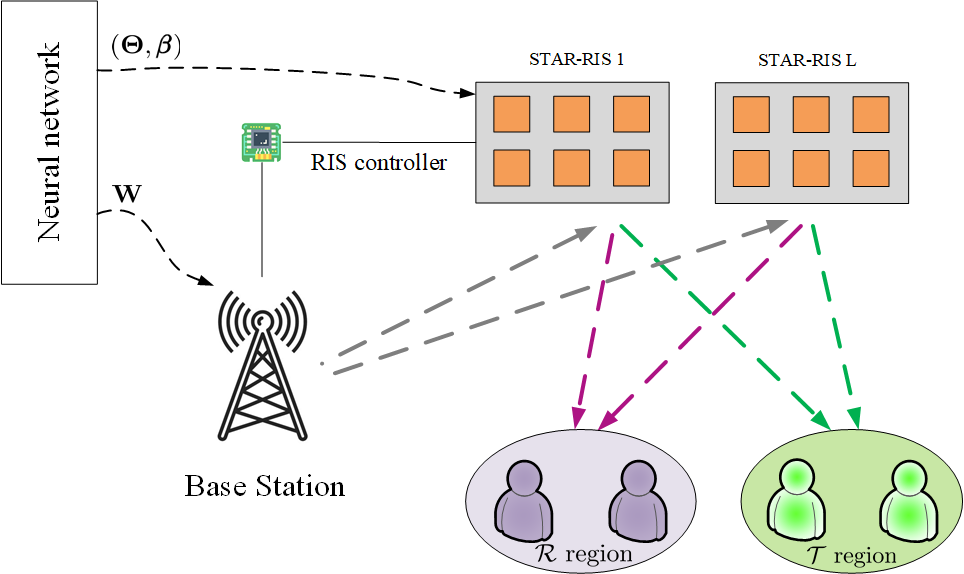
$(a)$

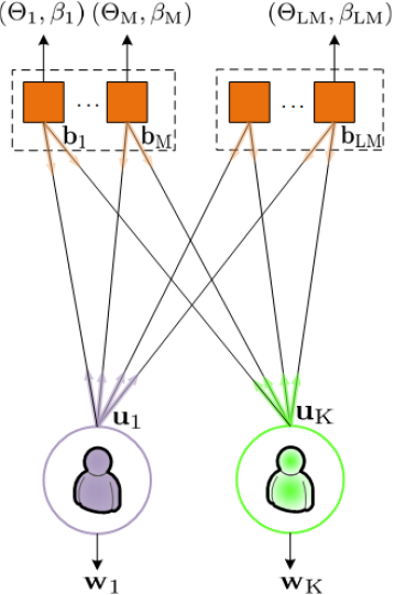
$(b)$

Figure 2: $(a)$ The proposed deep learning framework for the joint active and passive beamforming design problem. $(b)$ The graph representation of the distributed STAR-RISs systems.

This section presents the main contribution of the paper. Specifically, a GNN-based solution is introduced to address the considered sum rate optimization problem. We begin by depicting the STAR-RIS multi-user system using a heterogeneous graph. This graph comprises STAR-RIS vertices and user vertices, effectively capturing the dynamic interplay between users and STAR-RISs within the system. The overall deep learning framework is illustrated in Fig. 2$(a)$.

IV-A Properties of the joint beamforming design policy

We now show that the optimal active and passive beamforming policy enjoys permutation equivalence property. We start by re-writing the objective function in (4) as

$$\begin{split}\gamma_{k}&=\frac{|\sum_{l=1}^{L}\sum_{m=1}^{M}h_{klm}\phi_{lm}^{\chi}\mathbf{G}_{lm}\mathbf{w}_{k}|^{2}}{\sum_{j\in\mathcal{K},j\neq k}|\sum_{l=1}^{L}\sum_{m=1}^{M}h_{klm}\phi_{lm}^{\chi}\mathbf{G}_{lm}\mathbf{w}_{j}|^{2}+\sigma^{2}}\\ &=\frac{|\sum_{l=1}^{L}\sum_{m=1}^{M}\phi_{lm}^{\chi}\tilde{\mathbf{h}}_{klm}^{H}\mathbf{w}_{k}|^{2}}{\sum_{j\in\mathcal{K},j\neq k}|\sum_{l=1}^{L}\sum_{m=1}^{M}\phi_{lm}^{\chi}\tilde{\mathbf{h}}_{klm}^{H}\mathbf{w}_{j}|^{2}+\sigma^{2}},\end{split}$$ (22)

where $\mathbf{h}_{kl}=[h_{kl1},\cdots,h_{klM}]^{T}$, $\mathbf{G}_{lm}$ denotes the $m$-th row of $\mathbf{G}_{l}$, and $\tilde{\mathbf{h}}_{klm}^{H}=h_{klm}\mathbf{G}_{lm}\in\mathbb{C}^{1\times N_{t}}$ denoting the equivalent channel between the $m$-th element of the $l$-th STAR-RIS and the $k$-th user including the channel from BS. With the re-written objective function, one may view the original system as a system comprising STAR-RIS and users with the corresponding propagation channels between them. We will learn a joint optimal active and passive beamforming policy as

$$\{\mathbf{W}^{\ast},\boldsymbol{\Phi}^{\chi\ast}\}=F(\mathbf{H}),$$ (23)

where $F(.)$ is the optimal beamforming policy that is needed to be learned, $\mathbf{W}^{\ast}=[\mathbf{w}_{1}^{\ast},\cdots,\mathbf{w}_{K}^{\ast}]$ is the optimal beamforming matrix, $\boldsymbol{\Phi}^{\chi\ast}=[(\boldsymbol{\Phi}^{\chi\ast}_{1})^{T},\cdots,(\boldsymbol{\Phi}^{\chi\ast}_{L})^{T}]^{T}$ denotes the optimal STAR-RIS phase shift, and $\mathbf{H}$ is the equivalent channel matrix between STAR-RIS elements and users, which is expressed as

$$\mathbf{H}=\begin{pmatrix}\tilde{\mathbf{h}}_{111}&\cdots&\tilde{\mathbf{h}}_{K11}\\ \vdots&\vdots&\vdots\\ \tilde{\mathbf{h}}_{11M}&\cdots&\tilde{\mathbf{h}}_{K1M}\\ \vdots&\vdots&\vdots\\ \tilde{\mathbf{h}}_{1LM}&\cdots&\tilde{\mathbf{h}}_{KLM}\end{pmatrix}\in\mathbb{C}^{LM\times K}.$$ (24)

Before investigating the PI and PE properties of the joint active and passive beamforming optimization problem, we introduce the definition of these properties. Let us consider a multivariate function $\mathbf{Y}=f(\mathbf{X})$, and a permutation matrix $\mathbf{\Pi}$, the PI and PE properties of $f(\mathbf{X})$ is defined by the following definition.

Definition 1: For an arbitrary permutation of matrix $\mathbf{X}$, i.e, denoted by $\mathbf{\Pi}\mathbf{X}$, if $\mathbf{Y}=f(\mathbf{\Pi}\mathbf{X})$, then $\mathbf{Y}=f(\mathbf{X})$ exhibits permutation invariance to $\mathbf{X}$. Additionally, if $\mathbf{\Pi}\mathbf{Y}=f(\mathbf{\Pi}\mathbf{X})$, then $\mathbf{Y}=f(\mathbf{X})$ is permutation equivalent to $\mathbf{X}$.

To investigate the properties of the beamforming optimization problem, we first consider a simple example, where there are 2 STAR-RISs exploited to support two users as illustrated in Fig. 2$(b)$ with $L=K=2$. If the order of two STAR-RISs is swapped, the order of optimal passive beamforming $\boldsymbol{\Phi}_{1}^{\chi\ast}$ and $\boldsymbol{\Phi}_{2}^{\chi\ast}$ is also swapped. In contrast, the beamforming policy defined in (23) remains unchanged. In general, when the order of STAR-RISs is permuted, the optimal STAR-RIS phase shifts, and the rows of $\mathbf{H}$ are permuted to $\mathbf{\Pi}_{1}\boldsymbol{\Phi}^{\chi*}$, and $\mathbf{\Pi}_{1}\mathbf{H}$, respectively. Moreover, when the order of users is permuted, the optimal beamforming vectors and the columns of $\mathbf{\Pi}_{1}\mathbf{H}$ are permuted to $\mathbf{\Pi}_{2}\mathbf{W}^{\ast}$ and $\mathbf{\Pi}_{1}\mathbf{H}\mathbf{\Pi}_{2}^{T}$. Since the optimal active and passive beamforming optimization policy remains unchanged, we have

$$\mathbf{\Pi}_{1}\boldsymbol{\Phi}^{\chi*},\mathbf{\Pi}_{2}\mathbf{W}^{*}=F(\mathbf{\Pi}_{1}\mathbf{H}\mathbf{\Pi}_{2}^{T}).$$ (25)

In other words, the optimal beamforming policy is permutation equivariant. By identifying the PE of the beamforming policy, we can design a neural network that not only simply approximates the mapping between channel information and optimal solution, but also preserves this structural property.

IV-B Heterogeneous Graphical Representation of STAR-RIS systems

We now introduce a comprehensive graphical framework that sheds light on the dynamics of the considered distributed STAR-RIS multi-user system. As illustrated in Fig. 2$(b)$, the system may be represented as a heterogeneous graph denoted as $\mathcal{G}(\mathcal{V},\mathcal{E})$, where the STAR-RIS elements and users form two vertex sets denoted as $\mathcal{S}$ and $\mathcal{K}$, where $|\mathcal{S}|=LM$ and $|\mathcal{K}|=K$. In addition, $\mathcal{E}$ comprises the set of undirected edges $(s,k)$ connecting RIS element vertex $s$ and user vertex $k$, $\forall s\in\mathcal{S},k\in\mathcal{K}$. To more effectively capture the interaction between user vertices and RIS vertices in the wireless graph, we initially establish the characteristics for each vertex and edge. Intuitively, the connection between user $k$ and RIS $s$ can be described by using the instantaneous channel information linking them. However, this approach is unsuitable for distributed STAR-RIS systems due to two primary reasons: First, the inherent passive nature of STAR-RIS makes it infeasible to collect instantaneous individual CSI. Second, although the base station possesses instantaneous information on the equivalent channel as per (24), it is not explicitly represented in the proposed graphical model, despite being leveraged in the learning process. Consequently, utilizing instantaneous channel information for each edge in the presented HGNN model would inadequately encapsulate the interactions. In this light, it is suggested from (22) that the equivalent channels between STAR-RISs and users are sufficient for the optimization of beamforming and phase shift vectors.

To this end, we define the feature for the $(s,k)$ edge connecting the $s$-th RIS vertex and the $k$-th user vertex as

$$\mathbf{e}_{s,k}=[\mathrm{Re}(\mathbf{H}[s,k]),\mathrm{Im}(\mathbf{H}[s,k])],$$ (26)

where $\mathbf{H}[s,k]$ denotes the $(s,k)$-th element of matrix $\mathbf{H}$. The edge feature matrix of the whole graph is then defined as $\mathbf{E}=[\mathbf{e}_{s,k}]\in\mathbb{R}^{LM\times K\times 2N_{t}}$. In order to facilitate the exchange of information among vertices, we introduce a graph message passing (GMP) protocol. This protocol enables the dissemination of knowledge across the entire heterogeneous graph, allowing for the collaborative sharing of pertinent statistics required for optimizing the active and passive beamforming vectors. The GMP inference is processed through a series of the $T$ iterations. During each iteration, every vertex communicates with its neighboring vertices, which results in an update of its internal state by processing the received messages from its adjacent nodes. The update procedure of a vertex state during the $t$-th iteration can be defined as

• User vertex update:

  $$\mathbf{u}^{(t)}_{k}=\mathcal{U}^{t}(\mathbf{u}^{(t-1)}_{k},\mathbf{w}_{k}^{(t-1)},\mathbf{c}_{k}^{(t)}),$$ (27)

• RIS vertex update

  $$\mathbf{b}^{(t)}_{s}=\mathcal{B}^{t}(\mathbf{b}^{(t-1)}_{s},\Theta_{s}^{(t-1)},\beta_{s}^{(t-1)},\mathbf{d}_{s}^{(t)}),$$ (28)

where $\mathbf{u}^{(t)}_{k}$ and $\mathbf{b}^{(t)}_{s}$ are the vertex feature of the $k$-th user vertex and the $s$-th RIS vertex at the $t$-th iteration, respectively. In addition, $\mathcal{U}^{t}(\cdot)$ and $\mathcal{B}^{t}(\cdot)$ are user vertex and RIS vertex combination operators. Moreover, $\mathbf{c}_{i}^{t}$ and $\mathbf{d}_{i}^{t}$ are the aggregated messages from a vertex’s neighbors, which are given, respectively, by

$$\mathbf{c}_{k}^{(t)}=\mathrm{PL}_{s\in\mathcal{S}}\{\phi^{t}(\mathbf{b}_{s}^{(t-1)},\mathbf{u}_{k}^{(t-1)},\mathbf{e}_{s,k})\},$$ (29a)

$$\mathbf{d}_{s}^{(t)}=\mathrm{PL}_{k\in\mathcal{K}}\{\psi^{t}(\mathbf{u}_{k}^{(t-1)},\mathbf{b}_{s}^{(t-1)},\mathbf{e}_{s,k})\},$$ (29b)

where $\phi^{t}$ and $\psi^{t}$ are the aggregation operators at the user vertices and RIS vertices, and $\mathrm{PL}(.)$ is the pooling function which is dimensional-invariant. In (27) and (28), $\mathbf{w}_{k}^{(t-1)}$, $\Theta_{r}^{(t-1)}$, and $\beta_{r}^{(t-1)}$ are the predicted beamforming vectors, the RIS phase shift and its amplitude at the $(t-1)$-th iteration, which are updated, respectively, as

$$\mathbf{w}_{k}^{(t-1)} =\mathcal{W}(\mathbf{u}^{(t-1)}_{k}),\quad\forall k\in\mathcal{K},$$ (30a)

$$\Theta_{s}^{(t-1)} =\mathcal{C}(\mathbf{b}_{s}^{(t-1)}),\quad\forall s\in\mathcal{S},$$ (30b)

$$\beta_{s}^{(t-1)} =\mathcal{D}(\mathbf{b}_{s}^{(t-1)}),\quad\forall s\in\mathcal{S},$$ (30c)

where $\mathcal{W}(\cdot)$, $\mathcal{C}(\cdot)$, and $\mathcal{D}(\cdot)$ are the mapping functions. It is worth highlighting that our proposed BMP differs from the conventional message passing procedure described in [19] and [26]. In the conventional approach, optimized variables are only predicted at the last iteration, $T$, of the procedure. Additionally, both types of vertices utilize similar computation structures for the message generation rule. This may be sufficient in the power allocation problem considered in [19] where there is only one type of variable to be optimized, i.e. the power allocated at each antenna. However, in the joint beamforming design problem where various types of variables need to be jointly optimized, such a message generation rule lacks the capacity to capture the heterogeneous characteristics of the graph network. On the contrary, the proposed BMP predicts beamforming vectors and STAR-RIS phase shifts at each iteration and integrates them into a dedicated message generation rule for each vertex type. This information will be then propagated throughout the vertices and utilized in subsequent iterations for beamforming and phase shift prediction. The updated message passing enhances the performance of the designed graph neural network.

The proposed GMP hinges on the pooling function in (29), enabling the dimension-invariant computation of the graph. We apply the sum operator in the paper, which is a widely recognized and efficient pooling function utilized across various applications [18, 17]. The proposed GMP inference is presented in Algorithm 3.

Algorithm 3 Proposed GMP inference

1:Initialize $\mathbf{u}_{k}^{(0)},\mathbf{b}_{l}^{(0)},\forall k\in\mathcal{K},s\in\mathcal{S}$ and $t=0$.

2:for $t\leftarrow 1$ to $T$ do

1. User vertex update:

   The $k$-th user vertex aggregates its received messages from (29a) to generate message $\mathbf{c}_{k}^{(t)}$.

   The $k$-th user vertex updates its new feature $\mathbf{u}_{k}^{(t)}$ from (27) and sends it to the $s$-th RIS vertex $s\in\mathcal{S}$.

   The $k$-th user generates its corresponding beamforming vector as in (30a).

2. RIS vertex update:

   The $s$-th RIS vertex aggregates its received messages from (29b) to generate message $\mathbf{d}_{s}^{(t)}$.

   The $s$-th RIS vertex updates its new feature $\mathbf{b}_{s}^{(t)}$ from (28) and sends it to the $k$-th user vertex $k\in\mathcal{K}$.

   The $s$-th RIS vertex generates its phase shift and amplitude as in (30b) and (30c).

3:end for

4:Return the predicted beamforming vectors, RIS phase shift and amplitude at the $T$-th iteration.

IV-C Properties of the proposed GMP

This subsection discusses the key properties of the GMP that are favorable to handle the scalable joint beamforming optimization problems.

IV-C1 Permutation equivariance

The permutation equivariance property of the GMP is stated in Proposition 1.

Proposition 1.

Let the outputs of the GMP defined in (27) and (28) denote $\Phi:(\mathbf{E})\mapsto\mathbf{U},\mathbf{B}$, where $\mathbf{E}$ is the edge feature tensor, $\mathbf{U}$ and $\mathbf{B}$ are the outputs of the GMP corresponding to the user and RIS vertices, i.e., vertex features at the last layer of GMP. Also, For any $\mathbf{\Pi}_{1}$ and $\mathbf{\Pi}_{2}$ denoting RIS and user vertex permutation matrices, respectively, we have

$$\{\mathbf{\Pi}_{1}\mathbf{B},\mathbf{\Pi}_{2}\mathbf{U}\}=\Phi(\mathbf{\Pi}_{1}\mathbf{E}\mathbf{\Pi}_{2}^{T}),$$ (31)

Proof:

Refer to Appendix A. ∎

As demonstrated in the previous subsection, the active and passive beamforming policy exhibits a PE property, which indicates that an optimal solution obtained from a permuted problem corresponds to a permutation of the solution derived from the original problem. Proposition 1 confirms that the GMP adheres to this property. Specifically, if a GNN performs well on a particular input, it also delivers comparable performance on permutations of that input. It is important to highlight that this property is not inherently guaranteed by FCNNs or CNNs. In contrast, achieving permutation equivariance necessitates data augmentation during the training of FCNNs or CNNs, adding extra computational complexity.

IV-C2 Scalability to different system configurations

Due to the dimensional constraints, both FCNNs and CNNs must have the same input and output dimension in the training and testing phases. Therefore, the number of agents in the inference phase can not exceed those in the training phase, which limits the scalability of these networks to various system configurations when the number of UEs varies. In contrast, in the GMP, each vertex with the same type is processed by the same non-linear functions, i.e., $\mathcal{B}(\cdot),\mathbf{U}(\cdot),\phi^{t}(\cdot),$ and $\psi^{t}(\cdot)$, whose input dimension is invariant to the number of vertices. Thus, the GMP can be readily adapted to different scales of the considered problem in the testing phase

IV-D Implementation of Heterogeneous Graph Neural Network

In this section, we present an implementation of a beamforming heterogeneous graph neural network (BHGNN), which effectively executes the GMP inference described in Algorithm 2. Particularly, the BHGNN model contains $T$ layers corresponding to $T$ iterations of the proposed GMP inference. We focus on the implementation of the vertex operators, the aggregation operators, and the mapping functions at each BHGNN layer. Instead of finding the exact structure, we adopt various FCNNs to implicitly approximate these functions. The vertex operators and aggregation operators at the $t$-th layer are designed as

$$\begin{split}\mathbf{u}^{(t)}_{k}&=f_{\mathcal{U}}^{t}\big{(}\mathbf{u}^{(t-1)}_{k},\mathbf{w}_{k}^{(t-1)},\mathbf{c}_{k}^{(t)}\big{)},\\ \mathbf{b}^{(t)}_{s}&=f_{\mathcal{B}}^{t}(\mathbf{b}^{(t-1)}_{s},\Theta_{s}^{(t-1)},\beta_{s}^{(t-1)},\mathbf{d}_{s}^{(t)}),\\ \mathbf{c}_{k}^{(t)}&=\sum_{s\in\mathcal{S}}(f_{\phi}^{t}(\mathbf{b}_{s}^{(t-1)},\mathbf{u}_{k}^{(t-1)},\mathbf{e}_{s,k})),\\ \mathbf{d}_{s}^{(t)}&=\sum_{k\in\mathcal{K}}(f_{\psi}^{t}(\mathbf{u}_{k}^{(t-1)},\mathbf{b}_{s}^{(t-1)},\mathbf{e}_{s,k})),\\ &\mathbf{w}_{k}^{(t)}=f_{\mathcal{W}}(\mathbf{u}^{(t)}_{k}),\\ &\Theta_{s}^{(t)}=f_{\mathcal{C}}(\mathbf{b}_{s}^{(t)}),\\ &\beta_{s}^{(t)}=f_{\mathcal{D}}(\mathbf{b}_{s}^{(t)}),\end{split}$$ (32)

where $f(\cdot)$ is a FCNN. The reliability of these neural networks is substantiated by the universal approximation theorem [27], affirming that a properly constructed FCNN is able to approximate any continuous function with a sufficiently small error. After the $T$ layers, the beamforming vectors are gathered and normalized to satisfy the transmit power constraint as follows:

$$\begin{split}\mathbf{w}_{k}^{(T)}&=f_{\mathcal{W}}(\mathbf{u}^{(T)}_{k})\in\mathbb{R}^{2N_{t}},\\ \mathbf{W}^{(T)}&=[\mathbf{w}_{1}^{(T)},\cdots,\mathbf{w}_{K}^{(T)}]\in\mathbb{R}^{2N_{t}\times K},\\ \mathbf{W}^{(T)}&=\sqrt{P_{\mathrm{max}}}\frac{\mathbf{W}^{(T)}}{||\mathbf{W}^{(T)}||_{F}},\\ \mathbf{W}&=\mathbf{W}^{(T)}(1:N_{t},:)+j\mathbf{W}^{(T)}(N_{t}+1:2N_{t},:),\end{split}$$ (33)

where $\mathbf{W}(i_{1}:i_{2},:)$ denotes a matrix constructed by taking from the $i_{1}$-th to the $i_{2}$-th row of $\mathbf{W}$. Moreover, the STAR-RIS phase shift and amplitude in (2) are obtained as

$$\Theta_{s}^{(T)} =f_{\mathcal{C}}(\mathbf{b}_{s}^{(T)})\in\mathbb{R}^{2},\quad\forall s\in\mathcal{S},$$

$$\mathbf{\Theta}_{l}^{t} =e^{j2\pi[\Theta_{lM+1}^{(T)}(1),\cdots,\Theta_{(l+1)M}^{(T)}(1)]},\quad l\in\mathcal{L},$$

$$\mathbf{\Theta}_{l}^{r} =e^{j2\pi[\Theta_{lM+1}^{(T)}(2),\cdots,\Theta_{(l+1)M}^{(T)}(2)]},\quad l\in\mathcal{L},$$

$$\beta_{s}^{(T)} =f_{\mathcal{D}}(\mathbf{b}_{s}^{(T)})\in\mathbb{R},\quad\forall s\in\mathcal{S},$$

$$\boldsymbol{\beta}_{l}^{t} =\left[\sqrt{\beta_{lM+1}^{(T)}},\cdots,\sqrt{\beta_{(l+1)M}^{(T)}}\right],\quad l\in\mathcal{L},$$

$$\boldsymbol{\beta}_{l}^{r} =\left[\sqrt{1-\beta_{lM+1}^{(T)}},\cdots,\sqrt{1-\beta_{(l+1)M}^{(T)}}\right],\quad l\in\mathcal{L}.$$ (34)

It is worth noting that in the BHGNN architecture, all vertices employ an identical FCNN structure, which remains invariant regardless of the number of UEs or STAR-RISs. This attribute is crucial as it ensures that the BHGNN system can scale effectively, accommodating any number of users and STAR-RISs. This scalability distinguishes the BHGNN model from traditional DL models such as CNN and FCNN, where the system settings during the training and testing phases are required to remain unchanged. While increasing the depth of the FCNN within BHGNN may be necessary in larger system settings, even with fixed FCNNs, any performance degradation in BHGNN would be minimal. This ability to generalize across different scenarios will be confirmed in the simulation section.

IV-E Training the BHGNN

After obtaining the predicted variables as in (IV-D), the sum rate can be readily computed according to (3) and (4a). In order to train the proposed BHGNN, we define the training minimization problem on the negative expectation of the sum rate as

$$\underset{\mathbf{\Omega}\textperiodcentered}{\mathrm{minimize}}\quad-\mathbb{E}\left[\sum_{k=1}^{K}R_{k}(\mathbf{W},\mathbf{\Theta}^{\chi},\boldsymbol{\beta},\mathbf{\Omega})\right],$$ (35)

where $\mathbf{\Omega}=\{\boldsymbol{\omega}_{\mathcal{W}},\boldsymbol{\omega}_{\mathcal{D}},\boldsymbol{\omega}_{\mathcal{C}},\boldsymbol{\omega}_{\mathcal{U}},\boldsymbol{\omega}_{\mathcal{B}},\boldsymbol{\omega}_{\psi},\boldsymbol{\omega}_{\phi}\}$ is the set of the parameters of the FCNNs. The parameters update can be done using the established methods like the mini-batch SGD algorithm, along with its variants such as the ADAM algorithm. [28].

IV-F Complexity Analysis

This section analyzes the computational complexity of the proposed BHGNN model. As described above, the BHGNN model comprises multiple FCNN models. For a FCNN model with $H$ hidden layers, its computational complexity is given by [29]

$$C_{\mathrm{FCNN}}=\mathcal{O}\left(In_{1}+n_{H}N+\sum_{i=1}^{H-1}n_{i}n_{i+1}\right),$$ (36)

where $I$, $N$, and $n_{i}$ are the input size, the output size, and the number of neural in the $i$-th layers of the FCNN, respectively. Given the FCNN models designed for the HBGNN in Table I, and by considering the number of vertices of the HBGNN, the total computational complexity of the model is on the order of $\mathcal{O}(LMN_{t}^{2}+KN_{t}^{2}+TN_{t})$. Therefore, it becomes evident that the proposed HBGNN exibits lower complexity compared to the AO-based SCA algorithm.

V Numerical Results

This sections evaluates the performance of the distributed STAR-RIS-aided MU-MISO system for the proposed approaches. We also compare the distributed and centralized STAR-RIS systems under different aspects.

V-A Simulation Settings

We utilize a three-dimensional (3D) Cartesian coordinates to present the positions of devices in the considered system. The BS is situated at the origin, positioned at a height of $d_{H}$ meter (m), where the location of the $l$-th STAR-RIS is given by $(10\cdot l,0,d_{R})$. The locations of users are uniformly distributed on the ground in the rectangular area $[20,30]\times[20,30]$ (m) in the $(x,y)$-plane for the $\mathcal{T}$ users and $[-30,-20]\times[20,30]$ (m) in the $(x,y)$-plane for the $\mathcal{R}$ users. If not explicitly stated, we assume the number of BS antennas to be $N_{t}=16$ with the transmit power budget $P_{\mathrm{max}}=30$ dBm. The number of STAR-RISs is $L=4$, where the number of STAR-RIS elements varies according to the scenarios. The channels between the BS and STAR-RISs and between STAR-RISs and users follow the Rician fading channel models as

$$\mathbf{G}_{l} =\kappa_{1,l}\left(\sqrt{\frac{\xi}{\xi+1}}\bar{\mathbf{G}}_{l}+\sqrt{\frac{1}{\xi+1}}\tilde{\mathbf{G}}_{l}\right),$$ (37)

$$\mathbf{h}_{kl} =\kappa_{2,kl}\left(\sqrt{\frac{\xi}{\xi+1}}\bar{\mathbf{h}}_{kl}+\sqrt{\frac{1}{\xi+1}}\tilde{\mathbf{h}}_{kl}\right),$$

where $\kappa_{1,l}$ represents the distance path-loss of the channel link modeled as $32.6+36.7\log_{10}(d)$ dB, with $d$ signifies the channel link distance measured in meter, $\tilde{\mathbf{G}}_{l}$ and $\tilde{\mathbf{h}}_{kl}$ denote the non-light-of-sight (NLOS) components, which follow standard Gaussian distributions. In addition, $\bar{\mathbf{G}}_{l}$ and $\bar{\mathbf{h}}_{kl}$ denote the light-of-sight (LOS) components. We assume the BS antennas are arranged in a ULA structure, while STAR-RISs elements are arranged in the form of a UPA structure. Thus, the LoS components in (37) are expressed as the product of the UPA and ULA response vector as [30]

$$\begin{split}\bar{\mathbf{G}}_{l}&=\mathbf{a}_{R_{l}}(\theta^{A}_{TR_{l}},\phi^{A}_{TR_{l}})\mathbf{a}_{T}^{H}(\theta^{D}_{TR_{l}}),\\ \bar{\mathbf{h}}_{kl}&=\mathbf{a}_{R_{l}}(\theta^{D}_{R_{l}k},\phi^{D}_{R_{l}k}),\end{split}$$ (38)

where $\mathbf{a}_{R_{l}}(\theta^{A}_{TR_{l}},\phi^{A}_{TR_{l}})$ is the steering vector at the $l$-th STAR-RIS, $\mathbf{a}_{T}(\theta^{D}_{TR_{l}})$ is the steering vector at the BS, $(\theta^{A}_{TR_{l}},\phi^{A}_{TR_{l}})$ denote the azimuth and elevation angle-of-arrival (AoA) at the $l$-th STAR-RIS, $(\theta^{D}_{R_{l}k},\phi^{D}_{R_{l}k})$ presents the azimuth and elevation angle-of-departure (AoD) from the $l$-th STAR-RIS to the $k$-th user, and $\theta^{D}_{TR_{l}}$ is the AoD from the BS to the $l$-th STAR-RIS. In (38) the steering vectors are modelled as

$$\begin{split}&[\mathbf{a}_{R_{l}}(\theta^{A}_{TR_{l}},\phi^{A}_{TR_{l}})]_{n}=\\ &\quad\quad e^{j\frac{2\pi d_{RIS}}{\lambda}\{i_{1}(n)\mathrm{sin}(\theta^{A}_{TR_{l}})\cos(\phi^{A}_{TR_{l}})+i_{2}(n)\sin(\phi^{A}_{TR_{l}})\}},\\ &[\mathbf{a}_{T}(\theta^{D}_{TR_{l}})]_{n}=e^{j\frac{2\pi d_{A}(n-1)\sin(\phi^{A}_{TR_{l}})}{\lambda}},\end{split}$$ (39)

where $d_{RIS}$ is the distance between to consecutive STAR-RIS elements, $d_{A}=\lambda/2$ is the distance between BS antennas, with $\lambda$ denotes the carrier wavelength in meter, $i_{1}(n)=\mod(n-1,10),$ and $i_{2}(n)=\lfloor(n-1)/10\rfloor$. For the AO-based algorithm and the SCA method, we set the penalty factor as $C=10^{4}$, the convergence tolerance levels as $\epsilon=\epsilon_{1}=\epsilon_{3}=\epsilon_{2}=10^{-3}$. Moreover, we adopt a three-layer HBGNN model, i.e. $T=3$, with the deployment of the FCNN presented in Table I. To implement the proposed GNN model, we utilize the PyTorch deep learning library [31]. To train the proposed neural network, 50,000 channel realizations are generated as dataset, among which 45,000 channel realizations are used for the training phase and 5,000 realizations are used for the testing phase. The neural network is trained employing the ADAM optimizer [32], with an initial learning rate of $10^{-3}$. Throughout the training phase, the learning rate undergoes reduction every 10 epochs with a decay rate of 0.95. The training process ends when the validation loss fails to decrease consistently for five consecutive epochs.

TABLE I: Parameters of the designed fully connected layer networks

Name	Shape	Activation function
$f^{1}_{\phi}$, $f^{1}_{\psi}$	$2+2N_{t}\times 2+2N_{t}$	ReLU
$f^{2}_{\phi}$, $f^{3}_{\phi}$,$f^{2}_{\psi},f^{3}_{\psi}$	$574\times 574$	ReLU
$f^{1}_{\mathcal{U}}$, $f^{1}_{\mathcal{B}}$	$2+2N_{t}\times 256$	ReLU
$f^{2}_{\mathcal{U}}$, $f^{2}_{\mathcal{B}}$,$f^{3}_{\mathcal{U}}$, $f^{3}_{\mathcal{B}}$	$574\times 256$	ReLU
$f_{\mathcal{W}}$	$256\times 256\times 2N_{t}$	ReLU
$f_{\mathcal{C}}$	$256\times 64\times 2$	Sigmoid
$f_{\mathcal{D}}$	$256\times 64\times 1$	Sigmoid

To facilitate comparison, we present the performance of the following benchmarks:

1. AO-SCA: The iterative algorithm for solving problem (4) presented in Algorithm 2.

2. BHGNN: The proposed heterogeneous graph neural network presented in Section IV. Unless specified otherwise, the BHGNN is trained for the setting of $N_{t}=16,L=4,M=4$, and $K=8$, and is tested with different settings to show its generalizability capability robust to various settings.

3. Naive CNN: Conventional CNN design that processes the entire channel matrices $\mathbf{H}$ and $\mathbf{G}$. We follow a similar architecture in [33] where the beamforming vector, STAR-RIS phase shift, and amplitude are jointly optimized.

4. HetGNN: A heterogeneous GNN design with vertices and edges defined similarly to the proposed BHGNN. However, the conventional message passing procedure is adopted as in [19] to optimize the neural network.

5. Centralized STAR-RIS: We apply Algorithm 2 to optimize beamforming vectors, phase shift, and amplitude of the system with a single STAR-RIS located near the users. The total number of the single STAR-RIS elements is set to be equal to the total number of that in the distributed scenario, i.e. $LM$, for a fair comparison.

6. Random Phase shift: We optimize beamforming vectors with the method proposed in Algorithm 2, while the phase shift and amplitude of the STAR-RISs are randomized.

7. AO-SCA-EXH: We run the AO-SCA algorithm with different initialization points for a sufficiently large number and output the solution with the highest sum rate performance. Since Algorithm 2 is proved to converge to the KKT point of the approximated convex problem, this scheme is expected to approximate the global optimal solution of the approximated convex problem

V-B Performance Evaluation

We first evaluate convergence of BHGNN model during the training phase. In Fig. 3, we show the performance of BHGNN model on both training and validation dataset. Furthermore, the convergence of AO-SCA scheme is also presented for the comparison. As observed, the BHGNN model converges after approximately 40 epochs. Furthermore, its performance on the validation dataset eventually matches that of the AO-SCA benchmark.

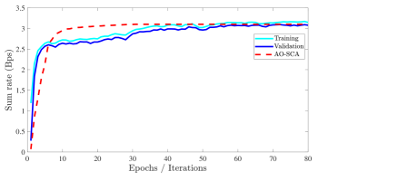
Figure 3: The training convergence of the proposed BHGNN model with $N_{t}=16,K=4,L=4,M=8$.

Next, we compare the sum rate performance of the examined benchmarks versus the number of total STAR-RIS elements in Fig. 4. In addition, to show the superiority of the distributed STAR-RIS system, we also present the performance of the single STAR-RIS-assisted system with an equal number of STAR-RIS elements. As can be observed, the random phase-shift benchmark still achieves a small gain, while the sum rate of the others examined frameworks grows significantly as the number of STAR-RIS elements grows. Particularly, the proposed BHGNN yield a comparable performance with the AO-SCA benchmarks, and the both schemes achieve near-performance compared to the AO-SCA-EXH scheme. As the number of STAR-RIS elements increases, the performance gap to the AO-SCA-EXH scheme becomes larger. This is straightforward since in higher dimensions, the optimization space is extremely large. The algorithm is, therefore, more likely to converge to a local optimal solution. While the BHGNN is trained with $(L,M)=(4,8)$, it shows a good generalizes capability robust to different numbers of STAR-RIS coefficients.

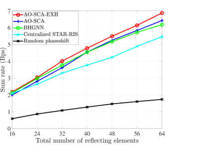
Figure 4: The sum rate performance versus total number of STAR-RIS elements of the examined methods, with $K=8,N_{t}=16$.

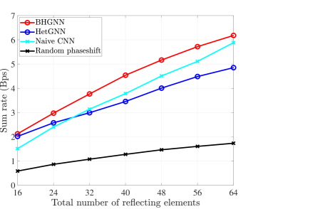
Figure 5: The sum rate performance versus total number of STAR-RIS elements of different ML-based methods, with $K=8,N_{t}=16$.

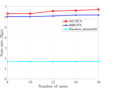
Figure 6: The sum rate performance versus number of users with $N_{t}=16$, $L=4$, $M=16$.

In Fig. 5, we compare the proposed BHGNN model with other existing deep learning designs. As illustrated, the proposed BHGNN outperforms other DL models. Although the Naive CNN model can achieve a close performance compared to BHGNN, it is required to be re-trained for different numbers of RIS elements. In addition, the performance of the HetGNN model is notably inferior to that of the the proposed BHGNN and the CNN model. This is because while the BHGNN and CNN models are designed for the joint beamforming design, HetGNN model is originally proposed for the conventional beamforming problem. The result also validates the effectiveness of our proposed message-passing inference. Furthermore, as shown in Fig. 6, the proposed BHGNN showcases a good generalization capability robust to different numbers of users, while achieving comparable performance to the AO-based algorithm. This is crucial since unlike the conventional DNN models, the proposed BHGNN does not require to be re-trained when the number of STAR-RIS elements and users are changed. Consequently, this feature enhances the practical utility of the proposed BHGNN in real environments.

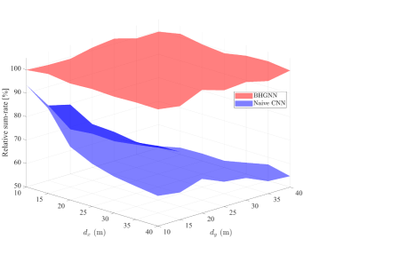
Figure 7: The sum rate performance versus different user location’s density, with $N_{t}=16$, $L=4$, $M=10$, $K=8$.

Fig. 7 illustrates the relative sum rate performance obtained by the proposed BHGNN and naive CNN model as a function of different user location densities. The relative sum rate is defined as the sum rate normalized by that of the AO-SCA algorithm. Specifically, the DL models are first trained as users are uniformly distributed in the rectangular area of $(x,y)=[\pm 20,\pm 30]\times[20,30]$ (m). We then vary the area of the rectangle in the testing phase as $(x,y)=[20,20+d_{x}]\times[20,20+d_{y}]$ (m) for $\mathcal{T}$ users and $(x,y)=[-20-d_{x},-20]\times[20,20+d_{y}]$ (m) for $\mathcal{R}$ users, where $d_{x}$ and $d_{y}$ denote the range of the location rectangle. Even though most of the user locations are unseen in the testing phase, the designed BHGNN obtains almost the same sum rate compared to the AO-SCA algorithm. In contrast, the naive CNN yields significant performance losses, particularly when the network area is larger. This validates the scalability to different network sizes of our proposed HGNN model. Unlike the naive CNN model which simply memorizes the mapping between channel information and the optimal solution, the BHGNN model learns the universal optimization rule which allows it to generalize well robust to different system configurations.

TABLE II: Average Running Time of the AO-SCA and BHGNN Approaches

Parameters	AO-SCA	BHGNN
$LM=16,K=4$	177.4 ms	25.7 ms
$LM=16,K=8$	288.1 ms	29.3 ms
$LM=16,K=16$	821.5ms	32.4 ms
$LM=64,K=4$	203.1 ms	26.6 ms
$LM=64,K=8$	414.1 ms	39.5 ms
$LM=64,K=16$	1271.7 ms	43.3 ms

Finally, we compare the computational complexity of the two proposed scheme in terms of average CPU running time in Table II. As illustrated, the BHGNN exhibits significantly slower running time compared to the AO-SCA. In addition, as the total number of STAR-RIS coefficients and users increases, the complexity of the BHGNN slightly increases, while the running time of AO-SCA grows drastically. This result aligns well with the complexity analysis presented in the previous sections.

VI Conclusion

In this paper, we delved into the joint optimization of active and passive beamforming in a distributed STAR-RIS assisted MU-MISO communication networks to maximize the overall sum rate. We proposed a novel GNN-based approach that efficiently handle the inherent non-convexity of the original problem. A HGNN model was designed to directly optimize the beamforming vectors and STAR-RIS elements, namely BHGNN. Particularly, we modeled each user and STAR-RIS coefficient as vertices, while the effective channel information was exploited as edges connecting them. Numerical results showed that the proposed BHGNN model can achieve a comparable sum rate performance to AO-based benchmark, and it can generalize well with different number of users as well as STAR-RIS coefficients. Furthermore, the BHGNN model requires significantly lower computational complexity compared to the AO-based benchmark, rendering it feasible for practical system implementations.

Appendix A Proof of Proposition 1

We represent the input features of user vertex $k$ and RIS vertex $s$ in the original graph as $\mathbf{u}_{k}^{(0)}$ and $\mathbf{b}_{s}^{(0)}$, respectively, the edge feature connecting RIS vertex $s$ and user vertex $k$ as $\mathbf{e}_{s,k}$, and the outputs of the $t$-th layer as $\mathbf{u}_{k}^{(t)}$ and $\mathbf{b}_{r}^{(t)}$. These variables in the permuted graph are correspondingly denoted as $\hat{\mathbf{u}}_{k}^{(0)}$, $\hat{\mathbf{b}}_{r}^{(0)}$, $\hat{\mathbf{e}}_{s,k}$, $\hat{\mathbf{u}}_{k}^{(t)}$, and $\hat{\mathbf{b}}_{r}^{(t)}$. At the initial stage of the graph, we have

$$\begin{split}\begin{gathered}\hat{\mathbf{e}}_{\pi_{1}(s),\pi_{2}(k)}=\mathbf{e}_{s,k},\quad\hat{\mathbf{b}}_{\pi_{1}(s)}^{(0)}=\mathbf{b}_{s}^{(0)},\quad\hat{\mathbf{u}}_{\pi_{2}(k)}^{(0)}=\mathbf{u}_{k}^{(0)},\\ \mathcal{S}(\pi_{1}(s))=\{\pi_{1}(s),s\in\mathcal{S}\},\quad\mathcal{K}(\pi_{2}(k))=\{\pi_{2}(k),k\in\mathcal{K}\},\end{gathered}\end{split}$$ (40)

where $\pi_{1}$ and $\pi_{2}$ are the permutation operator on the RIS vertices and user vertices. Specifically, these operators are defined as

$$\begin{split}\pi_{1}:[LM]\rightarrow[LM]\quad&\text{with}\quad[LM]=\{1,\ldots LM\}\\ \pi_{2}:[K]\rightarrow[K]\quad&\text{with}\quad[K]=\{1,\ldots,K\}\end{split}$$ (41)

For given permutation operators $\pi_{1}$, $\pi_{2}$ and $n$, we prove that $\mathbf{u}^{(n)}_{k}=\hat{\mathbf{u}}^{(n)}_{\pi_{2}(k)},\forall k$, and $\mathbf{b}^{(n)}_{s}=\hat{\mathbf{b}}^{(n)}_{\pi_{1}(s)},\forall n$ by induction. In the case of $n=0$, the proof directly follows (40). We now assume that the result holds with $n=1,\ldots,S-1$, that is

$$\begin{split}\begin{gathered}\mathbf{u}^{(n)}_{k}=\hat{\mathbf{u}}^{(n)}_{\pi_{2}(k)},\quad\mathbf{b}^{(n)}_{s}=\hat{\mathbf{b}}^{(n)}_{\pi_{1}(s)},\hat{\mathbf{e}}_{\pi_{1}(s),\pi_{2}(k)}=\mathbf{e}_{s,k},\\ \mathcal{S}(\pi_{1}(s))=\{\pi_{1}(s),s\in\mathcal{S}\},\quad\mathcal{K}(\pi_{2}(k))=\{\pi_{2}(k),k\in\mathcal{K}\},\\ \forall n=1,\ldots,S-1.\end{gathered}\end{split}$$ (42)

We prove that the results hold with $n=S$. Following the GMP update rule, the outputs of vertices at the $S$-th layer are

$$\mathbf{u}^{(S)}_{k}=\mathcal{U}^{S}\left(\mathbf{u}^{(S-1)}_{k},\mathcal{W}(\mathbf{u}^{(S-1)}_{k}),\right.$$

$$\left.\mathrm{PL}_{s\in\mathcal{S}}\left\{\phi^{S}(\mathbf{b}_{s}^{(S-1)},\mathbf{u}_{k}^{(S-1)},\mathbf{e}_{s,k})\right\}\right),$$

$$\hat{\mathbf{u}}^{s}_{\pi_{2}(k)}=\mathcal{U}^{S}\left(\mathbf{u}^{(S-1)}_{\pi_{2}(k)},\mathcal{W}(\mathbf{u}^{(S-1)}_{\pi_{2}(k)}),\right.$$

$$\quad\quad\left.\mathrm{PL}_{s\in\mathcal{S}(\pi_{1}(s))}\left\{\phi^{S}(\mathbf{b}_{r}^{(S-1)},\mathbf{u}_{\pi_{2}(k)}^{(S-1)},\mathbf{e}_{s,\pi_{2}(k)})\right\}\right),$$

$$\mathbf{b}^{(S)}_{s}=\mathcal{B}^{S}\left(\mathbf{b}^{(S-1)}_{s},\mathcal{C}(\mathbf{b}_{s}^{(S-1)}),\mathcal{D}(\mathbf{b}_{s}^{(S-1)}),\right.$$

$$\quad\quad\left.\mathrm{PL}_{k\in\mathcal{K}}\left\{\psi^{S}(\mathbf{u}_{k}^{(S-1)},\mathbf{b}_{s}^{(S-1)},\mathbf{e}_{s,k})\right\}\right)$$

$$\hat{\mathbf{b}}_{\pi_{1}(s)}^{(S)}=\mathcal{B}^{S}\left(\mathbf{b}^{(S-1)}_{\pi_{1}(s)},\mathcal{C}(\mathbf{b}_{\pi_{1}(s)}^{(S-1)}),\mathcal{D}(\mathbf{b}_{\pi_{1}(s)}^{(S-1)}),\right.$$

$$\quad\quad\left.\mathrm{PL}_{k\in\mathcal{K}(\pi_{2}(k))}\left\{\psi^{S}(\mathbf{u}_{k}^{(S-1)},\mathbf{b}_{\pi_{1}(s)}^{(S-1)},\mathbf{e}_{{\pi_{1}(s)},k})\right\}\right).$$ (43)

Plugging (42) into (A), we have $\mathbf{u}_{k}^{(S)}=\hat{\mathbf{u}}_{\pi(k)}^{(S)}$ and $\mathbf{b}_{s}^{(S)}=\hat{\mathbf{b}}_{\pi(s)}^{(S)}$. We recall that for the original graph, the output at RIS vertices is $\mathbf{U}=[\mathbf{u}_{1},\ldots,\mathbf{u}_{|\mathcal{S}|}]^{T}$, while that of the permuted graph is $\hat{\mathbf{U}}=[\hat{\mathbf{u}}_{1},\ldots,\hat{\mathbf{u}}_{|\mathcal{S}|}]^{T}$. Therefore, we have $\mathbf{U}=\pi_{1}\star\hat{\mathbf{U}}$, where $\pi_{1}\star\mathbf{A}$ is defined as $(\pi_{1}\star\mathbf{A})_{(\pi_{1}(i))}=\mathbf{A}_{(i)}$ for any matrix $\mathbf{A}$. Similarly, we have $\mathbf{B}=\pi_{2}\star\hat{\mathbf{B}}$, where $(\pi_{2}\star\hat{\mathbf{B}})_{\pi_{2}(i)}=\hat{\mathbf{B}}_{(s)}$. Since permutation of the output of the original graph is the output of the permuted graph, the result in proposition 1 is proved.

References

- [1] W. Saad, M. Bennis, and M. Chen, “A vision of 6g wireless systems: Applications, trends, technologies, and open research problems,” IEEE Network, vol. 34, no. 3, pp. 134–142, 2020.
- [2] E. Basar, M. Di Renzo, J. De Rosny, M. Debbah, M.-S. Alouini, and R. Zhang, “Wireless communications through reconfigurable intelligent surfaces,” IEEE Access, vol. 7, pp. 116 753–116 773, 2019.
- [3] X. Mu, Y. Liu, L. Guo, J. Lin, and R. Schober, “Simultaneously transmitting and reflecting (star) ris aided wireless communications,” IEEE Transactions on Wireless Communications, vol. 21, no. 5, pp. 3083–3098, 2022.
- [4] T. Wang, F. Fang, and Z. Ding, “Joint phase shift and beamforming design in a multi-user miso star-ris assisted downlink noma network,” IEEE Transactions on Vehicular Technology, vol. 72, no. 7, pp. 9031–9043, 2023.
- [5] C. Wu, Y. Liu, X. Mu, X. Gu, and O. A. Dobre, “Coverage characterization of star-ris networks: Noma and oma,” IEEE Communications Letters, vol. 25, no. 9, pp. 3036–3040, 2021.
- [6] A. Papazafeiropoulos, C. Pan, A. Elbir, P. Kourtessis, S. Chatzinotas, and J. M. Senior, “Coverage probability of distributed irs systems under spatially correlated channels,” IEEE Wireless Communications Letters, vol. 10, no. 8, pp. 1722–1726, 2021.
- [7] P. Wang, J. Fang, X. Yuan, Z. Chen, and H. Li, “Intelligent reflecting surface-assisted millimeter wave communications: Joint active and passive precoding design,” IEEE Transactions on Vehicular Technology, vol. 69, no. 12, pp. 14 960–14 973, 2020.
- [8] Z. Yang, M. Chen, W. Saad, W. Xu, M. Shikh-Bahaei, H. V. Poor, and S. Cui, “Energy-efficient wireless communications with distributed reconfigurable intelligent surfaces,” IEEE Transactions on Wireless Communications, vol. 21, no. 1, pp. 665–679, 2022.
- [9] J. Lee, H. Seo, and W. Choi, “Computation-efficient reflection coefficient design for graphene-based ris in wireless communications,” IEEE Transactions on Vehicular Technology, vol. 73, no. 3, pp. 3663–3677, 2024.
- [10] J. Gao, C. Zhong, X. Chen, H. Lin, and Z. Zhang, “Unsupervised learning for passive beamforming,” IEEE Communications Letters, vol. 24, no. 5, pp. 1052–1056, 2020.
- [11] H. An Le, T. Van Chien, V. D. Nguyen, and W. Choi, “Double ris-assisted mimo systems over spatially correlated rician fading channels and finite scatterers,” IEEE Transactions on Communications, vol. 71, no. 8, pp. 4941–4956, 2023.
- [12] W. Xu, L. Gan, and C. Huang, “A robust deep learning-based beamforming design for RIS-assisted multiuser MISO communications with practical constraints,” IEEE Transactions on Cognitive Communications and Networking, vol. 8, no. 2, pp. 694–706, 2022.
- [13] R. Zhong, Y. Liu, X. Mu, Y. Chen, X. Wang, and L. Hanzo, “Hybrid reinforcement learning for star-riss: A coupled phase-shift model based beamformer,” IEEE Journal on Selected Areas in Communications, vol. 40, no. 9, pp. 2556–2569, 2022.
- [14] J. Zhou, G. Cui, S. Hu, Z. Zhang, C. Yang, Z. Liu, L. Wang, C. Li, and M. Sun, “Graph neural networks: A review of methods and applications,” AI Open, vol. 1, pp. 57–81, 2020.
- [15] Y. Shen, J. Zhang, S. H. Song, and K. B. Letaief, “Graph neural networks for wireless communications: From theory to practice,” IEEE Transactions on Wireless Communications, vol. 22, no. 5, pp. 3554–3569, 2023.
- [16] M. Eisen and A. Ribeiro, “Optimal wireless resource allocation with random edge graph neural networks,” IEEE Transactions on Signal Processing, vol. 68, pp. 2977–2991, 2020.
- [17] Y. Shen, Y. Shi, J. Zhang, and K. B. Letaief, “Graph neural networks for scalable radio resource management: Architecture design and theoretical analysis,” IEEE Journal on Selected Areas in Communications, vol. 39, no. 1, pp. 101–115, 2021.
- [18] A. Chowdhury, G. Verma, C. Rao, A. Swami, and S. Segarra, “Unfolding wmmse using graph neural networks for efficient power allocation,” IEEE Transactions on Wireless Communications, vol. 20, no. 9, pp. 6004–6017, 2021.
- [19] J. Guo and C. Yang, “Learning power allocation for multi-cell-multi-user systems with heterogeneous graph neural networks,” IEEE Transactions on Wireless Communications, vol. 21, no. 2, pp. 884–897, 2022.
- [20] J. Kim, H. Lee, S.-E. Hong, and S.-H. Park, “A bipartite graph neural network approach for scalable beamforming optimization,” IEEE Transactions on Wireless Communications, vol. 22, no. 1, pp. 333–347, 2023.
- [21] T. Jiang, H. V. Cheng, and W. Yu, “Learning to reflect and to beamform for intelligent reflecting surface with implicit channel estimation,” IEEE Journal on Selected Areas in Communications, vol. 39, no. 7, pp. 1931–1945, 2021.
- [22] Z.-Q. Luo and S. Zhang, “Dynamic spectrum management: Complexity and duality,” IEEE journal of selected topics in signal processing, vol. 2, no. 1, pp. 57–73, 2008.
- [23] A. Zappone, E. Björnson, L. Sanguinetti, and E. Jorswieck, “Globally optimal energy-efficient power control and receiver design in wireless networks,” IEEE Transactions on Signal Processing, vol. 65, no. 11, pp. 2844–2859, 2017.
- [24] M. S. Lobo, L. Vandenberghe, S. Boyd, and H. Lebret, “Applications of second-order cone programming,” Linear Algebra and its Applications, vol. 284, no. 1, pp. 193–228, 1998.
- [25] X. Yang, M. Yan, S. Pan, X. Ye, and D. Fan, “Simple and efficient heterogeneous graph neural network,” ser. AAAI’23/IAAI’23/EAAI’23. AAAI Press, 2023. [Online]. Available: https://doi.org/10.1609/aaai.v37i9.26283
- [26] X. Zhang, H. Zhao, J. Xiong, X. Liu, L. Zhou, and J. Wei, “Scalable power control/beamforming in heterogeneous wireless networks with graph neural networks,” in 2021 IEEE Global Communications Conference (GLOBECOM), 2021, pp. 01–06.
- [27] K. Hornik, M. Stinchcombe, and H. White, “Multilayer feedforward networks are universal approximators,” Neural Networks, vol. 2, no. 5, pp. 359–366, 1989.
- [28] D. P. Kingma and J. Ba, “Adam: A method for stochastic optimization,” in 3rd International Conference on Learning Representations, ICLR 2015, San Diego, CA, USA, May 7-9, 2015, Conference Track Proceedings, Y. Bengio and Y. LeCun, Eds., 2015.
- [29] H. A. Le, T. Van Chien, T. H. Nguyen, H. Choo, and V. D. Nguyen, “Machine learning-based 5g-and-beyond channel estimation for mimo-ofdm communication systems,” Sensors, vol. 21, no. 14, 2021.
- [30] S. Zhang and R. Zhang, “Capacity characterization for intelligent reflecting surface aided MIMO communication,” IEEE Journal on Selected Areas in Communications, vol. 38, no. 8, pp. 1823–1838, 2020.
- [31] A. Paszke, S. Gross, F. Massa, A. Lerer, J. Bradbury et al., “Pytorch: An imperative style, high-performance deep learning library,” in Advances in Neural Information Processing Systems 32. Curran Associates, Inc., 2019, pp. 8024–8035.
- [32] D. P. Kingma and J. Ba, “Adam: A method for stochastic optimization,” CoRR, vol. abs/1412.6980, 2014. [Online]. Available: https://api.semanticscholar.org/CorpusID:6628106
- [33] H. Song, M. Zhang, J. Gao, and C. Zhong, “Unsupervised learning-based joint active and passive beamforming design for reconfigurable intelligent surfaces aided wireless networks,” IEEE Communications Letters, vol. 25, no. 3, pp. 892–896, 2021.