PINT: Maximum-likelihood estimation of pulsar timing noise parameters

Abstract

PINT is a pure-Python framework for high-precision pulsar timing developed on top of widely used and well-tested Python libraries, supporting both interactive and programmatic data analysis workflows. We present a new frequentist framework within PINT to characterize the single-pulsar noise processes present in pulsar timing datasets. This framework enables the parameter estimation for both uncorrelated and correlated noise processes as well as the model comparison between different timing and noise models. We demonstrate the efficacy of the new framework by applying it to simulated datasets as well as a real dataset of PSR B1855+09. We also briefly describe the new features implemented in PINT since it was first described in the literature.

1 Introduction

Since their discovery, pulsars have been used as celestial laboratories to probe a wide range of time-domain phenomena owing to their remarkable rotational stability. This is especially true for millisecond pulsars (MSPs), which are pulsars with millisecond-scale rotational periods spun up by accretion from a companion star (Manchester, 2017). Such applications include constraints on the neutron star equation of state (e.g. Cromartie et al., 2020), discovery of exoplanets (Wolszczan & Frail, 1992), tests of theories of gravity (e.g. Kramer et al., 2021), probing the interstellar medium (e.g. Donner et al., 2020) and solar wind (e.g. Tiburzi et al., 2021), creation of an international time standard (Hobbs et al., 2019), characterizing the uncertainties present in the solar system ephemerides (e.g. Caballero et al., 2018), and more. These exciting results were produced with the help of pulsar timing, the technique of tracking a pulsar’s rotational phase using the measured times of arrival (TOAs) of its pulses, allowing it to be used as a celestial clock (Lorimer & Kramer, 2012). Pulsar timing was instrumental in the recent evidence for a nanohertz gravitational wave background (Agazie et al., 2023b; Antoniadis et al., 2023; Reardon et al., 2023; Xu et al., 2023; Agazie et al., 2023) by Pulsar Timing Array (PTA) experiments (Sazhin, 1978; Foster & Backer, 1990), inaugurating the era of nanohertz gravitational wave astronomy.

High-precision pulsar timing experiments such as PTAs and tests of gravity require modeling the TOAs down to nanosecond-level precision. A pulsar timing model or pulsar ephemeris is a generative mathematical description of the deterministic astrophysical processes influencing the measured TOAs. These processes include pulsar rotation, pulsar binary dynamics, interstellar dispersion, solar system dynamics, proper motion, solar wind, etc., and must be accurately incorporated into the timing model to achieve the required precision (Edwards et al., 2006). The timing model is often accompanied by a noise model, which incorporates stochastic processes affecting the TOAs such as radiometer noise, pulse jitter, rotational irregularities, interstellar medium variability, radio frequency interference (RFI), etc (Agazie et al., 2023a).

In practice, pulsar timing involves the creation and incremental refinement of a pulsar timing model that matches the observed TOAs, typically using frequentist methods. This is usually performed using one of the three standard software packages: tempo (Nice et al., 2015), tempo2 (Hobbs et al., 2006; Edwards et al., 2006), and PINT (Luo et al., 2021), often in an interactive manner. Noise characterization is usually performed separately in the Bayesian paradigm using software packages such as ENTERPRISE (Johnson et al., 2023) and TEMPONEST (Lentati et al., 2014), starting from a post-fit timing model. ENTERPRISE can also be used to characterize deterministic and stochastic signals common across multiple pulsars, such as the stochastic gravitational wave background and solar system ephemeris errors (e.g. Agazie et al., 2023b; Vallisneri et al., 2020). However, for ease of use it would be useful to incorporate single-pulsar noise characterization in the same analysis used for the timing fit.

PINT is a flexible pure-Python framework for pulsar timing that is written on top of widely-used scientific computing libraries such as numpy (Harris et al., 2020), scipy (Virtanen et al., 2020), astropy (Price-Whelan et al., 2022), and matplotlib (Hunter, 2007), developed under the aegis of the North American Nanohertz Observatory for Gravitational Waves (NANOGrav: Demorest et al., 2012). The reliability of this package is ensured via its reliance on these well-tested libraries, strict version control, and an extensive continuous integration and testing suite. PINT is primarily designed to be used as a Python library to ensure that (a) all of its functionality remains easily accessible to the user, (b) it is easily extensible, and (c) it can be easily composed with other Python packages. It also provides a graphical user interface (named pintk) and command-line tools for specific tasks. In comparison, tempo and tempo2, written in FORTRAN and C-style C++ respectively, are primarily designed to be used as command-line applications (tempo2 also has a graphical user interface named plk and a Python wrapper named libstempo; Vallisneri 2020).

In this work, we present a new frequentist framework in PINT for characterizing the noise processes affecting pulsar timing, allowing the noise parameters to be fit simultaneously with the timing model parameters in a maximum-likelihood way for a single pulsar. This framework also enables model comparisons within PINT using the Akaike Information Criterion (AIC: Burnham & Anderson, 2004). The new framework should allow us to more easily incorporate noise characterization into interactive pulsar timing workflows and pulsar timing pipelines, obtaining relatively quick noise estimates. This is in contrast to conventional Bayesian noise characterization, which is performed as a separate step from pulsar timing and is relatively more computationally expensive but can also include common noise terms between pulsars (e.g. Agazie et al., 2023a). While this framework is not intended to replace Bayesian methods for noise characterization, it can nevertheless complement the Bayesian methods in the following ways. The quick noise estimates can help iteratively refine noise models and can be used as cross-checks for Bayesian results. They can also act as starting points for Markov Chain Monte Carlo (MCMC) samplers (e.g. Jones & Qin, 2022) allowing them to burn in faster.

This paper is arranged as follows. Section 2 provides a quick overview of pulsar timing. Section 3 briefly describes the fitting methods used in PINT. The newly implemented methods for estimating noise parameters are described in section 4. Model comparison using the AIC is described in section 5. We demonstrate the new framework using simulations in section 6, and using a real dataset in section 7. In section 8, we discuss some of the new developments in PINT, implemented since the publication of Luo et al. (2021) which initially described the package. Finally, we summarize our work in section 9.

2 A brief overview of pulsar timing

2.1 TOAs

The primary measurable quantity in pulsar timing is the TOA. In conventional pulsar timing, the pulsar time series data is coherently averaged (‘folded’) into an integrated pulse profile to improve its signal-to-noise ratio (S/N) and to mitigate the effects of pulse-to-pulse variations (Lorimer & Kramer, 2012). A TOA can be measured from an integrated pulse profile by matching it against a noise-free template (Taylor, 1992). In the traditional narrowband paradigm, the observation is split into multiple frequency sub-bands, and the TOAs are estimated in each sub-band independently. On the other hand, in the more recently developed wideband paradigm, a frequency-resolved integrated pulse profile is cross-correlated against a 2-dimensional template in frequency and pulse phase to simultaneously measure a TOA and a dispersion measure (DM) for the whole observation (Pennucci et al., 2014; Pennucci, 2019). Algorithms for folding and manipulating integrated pulse profiles and for measuring TOAs are available in packages like DSPSR (van Straten & Bailes, 2011), PRESTO (Ransom, 2001), PSRCHIVE (Hotan et al., 2004), and PulsePortraiture (Pennucci et al., 2014; Pennucci, 2019). We restrict ourselves to the narrowband paradigm in this work for the sake of simplicity unless explicitly stated otherwise.

The TOAs are generally recorded against local observatory clocks. PINT applies a series of clock corrections to the measured TOAs, bringing them to the Barycentric Dynamical Time (TDB), a relativistic timescale defined at the solar system barycenter (SSB). Detailed descriptions of clock corrections may be found in Hobbs et al. (2006) and Luo et al. (2021). Note that tempo2 uses the Barycentric Coordinate Time (TCB) by default, which differs from TDB by a constant factor, and timing models using TCB need to be converted to TDB to be PINT-compatible (see section 8.1 for the newly-available TCB to TDB conversion feature).

In PINT, a set of observed TOAs are represented by the TOAs class in the pint.toa module. See Luo et al. (2021) for details on the internal representation of TOAs. They are usually stored in human-readable text files known as ‘tim’ files. A ‘tim’ file can be read using the pint.toa.get_TOAs() function.

2.2 The timing and noise model

Pulsar timing involves connecting the pulse number $N$, related to the rotational phase of the pulsar as $\Phi(N)=2\pi N$, to the time of emission $t_{\text{em}}$ as

$$N=N_{0}+f(t_{\text{em}}-t_{0})+\frac{1}{2}\dot{f}(t_{\text{em}}-t_{0})^{2}+...\,,$$ (1)

where $f$ is the rotational frequency, $\dot{f}$ is the rotational frequency derivative, and $t_{0}$ is a fiducial time. The right-hand side of the above equation may also include higher-order frequency derivative terms as well as rotational irregularity effects such as glitches (Hobbs et al., 2006). The measured TOA $t_{\text{arr}}$ is related to $t_{\text{em}}$ by

$$t_{\text{arr}}=t_{\text{em}}+\Delta_{\text{B}}+\Delta_{\text{DM}}+\Delta_{\text{\astrosun}}+...+\mathcal{N}\,.$$ (2)

Here, the delay $\Delta_{\text{B}}$ originates from the motion of the pulsar in a binary system and includes Rømer delay, Shapiro delay, and Einstein delay (Damour & Deruelle, 1986). $\Delta_{\text{DM}}$ denotes the delay caused by interstellar dispersion and is given by $\Delta_{\text{DM}}=\mathcal{K}D/\nu^{2}$, where $\nu$ is the observing frequency, $D$ is the DM, and $\mathcal{K}$ is known as the DM constant (Lorimer & Kramer, 2012). $\Delta_{\text{\astrosun}}$ denotes the delays caused by the Solar System motion, including the Rømer delay and the Shapiro delay, and are computed using the solar system ephemerides published by space agencies (e.g., Park et al., 2021). A detailed description of the various timing model components can be found in Edwards et al. (2006) and Luo et al. (2021). Finally, $\mathcal{N}$ denotes the noise present in the TOA, including correlated and uncorrelated noise components (see section 4.1).

The various timing model components available in PINT are listed in Table LABEL:tab:model-components, and the new/updated components are highlighted therein. These are available in the pint.models module of PINT. The timing model as a whole, comprising these components, is represented by the TimingModel class in the pint.models module. Pulsar ephemerides are usually stored in human-readable text files known as ‘par’ files, and can be read using the pint.models.get_model() function. A pair of ‘par’ and ‘tim’ files belonging to the same pulsar can be read together using the pint.models.get_model_and_toas() function.

Table 1: Updated list of timing model components available in PINT (in the pint.models module). ‘§’ denotes newly implemented components. ‘†’ denotes components that have had significant changes since the publication of Luo et al. (2021). The BinaryELL1 component now includes up to $\mathcal{O}(e^{3})$ terms in orbital eccentricity. The SolarWindDispersion component now allows electron density radial power law indices other than 2. The EcorrNoise component now incorporates a faster algorithm for inverting the TOA covariance matrix. ‘¶’ denotes components that were renamed after the publication of Luo et al. (2021). ‘‡’ denotes components only available in PINT. The choice of the binary model is specified in the ‘par’ files using the ‘BINARY’ keyword, e.g., ‘BINARY ELL1’. Additionally, there is a generic timing model in tempo2 called the ‘T2’ model, which chooses the underlying binary model based on the available binary parameters. When ‘BINARY T2’ is encountered, PINT emits an informative error message indicating the best guess for the underlying binary model, and optionally constructs the binary timing model based on this guess.

Component	Description	References
Pulsar rotation, rotational phase & rotational irregularities
Spindown	Taylor series representation of the pulsar rotation	Backer & Hellings (1986)
PiecewiseSpindown §	Piecewise-constant corrections to pulsar rotation
Glitch	Pulsar glitches	Hobbs et al. (2006)
IFunc	Piecewise-constant or spline representation of rotational period	Deng et al. (2012)
WaveX §‡	Fourier series representation of achromatic red noise	Hobbs et al. (2006)
	(supersedes the deprecated Wave model)	Section 4.1.3, 4.3
PLRedNoise	Fourier Gaussian process representation of achromatic red	Lentati et al. (2014)
	noise
AbsPhase	Reference TOA with respect to which the rotational phase
	is measured
PhaseOffset §‡	Overall phase offset between reference TOA and the physical	Section 4.2
	TOAs
PhaseJump ¶	Phase offsets between TOAs measured using different systems	Hobbs et al. (2006)
Binary system
BinaryBT	Simple parametrized post-Keplerian binary model	Blandford & Teukolsky (1976)
	(only Rømer delay)
BinaryBTPiecewise §‡	Similar to BinaryBT, but with piecewise-constant
	orbital parameters
BinaryDD	Parametrized post-Keplerian model (with Shapiro	Damour & Deruelle (1986)
	delay and Einstein delay)
BinaryDDGR §	Similar to BinaryDD, but assumes General Relativity	Taylor & Weisberg (1989)
BinaryDDH §	Similar to BinaryDD, but uses a harmonic representation	Freire & Wex (2010)
	of Shapiro delay (for low-inclination systems)	Weisberg & Huang (2016)
BinaryDDK	Similar to BinaryDD, but includes Kopeikin delay	Damour & Taylor (1992)
		Kopeikin (1995, 1996)
BinaryDDS §	Similar to BinaryDD, but uses an alternative representation	Kramer et al. (2006)
	of Shapiro delay (for almost edge-on orbits)	Rafikov & Lai (2006)
BinaryELL1 †	Binary model specialized for nearly circular orbits using	Lange et al. (2001)
	Laplace-Lagrange parameters (includes up to third-order	Zhu et al. (2018)
	terms in eccentricity)	Fiore et al. (2023)
BinaryELL1H	Similar to ELL1, but uses a harmonic representation of	Freire & Wex (2010)
	Shapiro delay (for low-inclination systems)
BinaryELL1k §	Similar to ELL1, but includes an exact treatment of advance	Susobhanan et al. (2018)
	of periastron (for highly relativistic or tidally interacting
	binaries)
Interstellar dispersion & dispersion measure variations
DispersionDM ¶	Taylor series representation of dispersion measure (DM)	Backer & Hellings (1986)
DispersionDMX ¶	Piecewise-constant representation of DM variations	Arzoumanian et al. (2015)
DMWaveX §‡	Fourier series representation of DM variations	Section 4.1.3, 4.3
PLDMNoise §	Fourier Gaussian process representation of DM	Lentati et al. (2014)
	variations
DispersionJump §	Offsets between wideband DMs measured using different	Alam et al. (2021)
	systems (no delay)
FDJumpDM §	DM offsets between narrowband TOAs measured using different
	systems
Astrometry & solar system delays
AstrometryEcliptic	Astrometry in ecliptic coordinates	Edwards et al. (2006)
AstrometryEquatorial	Astrometry in equatorial coordinates
SolarSystemShapiro	Solar system Shapiro delay	Shapiro (1964)
Solar wind
SolarWindDispersion †	Solar wind model assuming a radial power-law relation for	Edwards et al. (2006)
	the electron density	You et al. (2007, 2012)
SolarWindDispersionX §‡	Similar to SolarWindDispersion, but with a piecewise-constant	Madison et al. (2019)
	representation of the electron density.	Hazboun et al. (2022)
Troposphere
TroposphereDelay	Tropospheric zenith hydrostatic delay	Davis et al. (1985)
		Niell (1996)
Time-uncorrelated noise
ScaleToaError	Modifications to the measured TOA uncertainties	Lentati et al. (2014)
ScaleDMError §	Modifications to the measured wideband DM uncertainties	Alam et al. (2021)
EcorrNoise †	Correlation between TOAs measured from the same	Arzoumanian et al. (2015)
	observation.	Johnson et al. (2023)
Frequency-dependent profile evolution
FD ¶	Frequency-dependent profile evolution	Arzoumanian et al. (2015)
FDJump §	System and frequency-dependent profile evolution	Appendix A

2.3 Timing residuals

The timing model can be used to predict the phase $\Phi_{i}$ associated with each TOA, and this allows us to compute the timing residuals

$$r_{i}=\frac{\Phi_{i}-2\pi N[\Phi_{i}]}{f_{i}}\,,$$ (3)

where $N[\Phi_{i}]$ is the integer closest to $\Phi_{i}/2\pi$, and $f_{i}$ is the instantaneous pulsar rotational frequency. The procedure for computing a timing residual can be summarized as follows:

1. Apply the various clock corrections to convert the measured TOA from the observatory timescale to a solar system barycenter (SSB) timescale.

2. Successively correct for the various delays influencing the TOA, bringing it to the pulsar frame (equation 2).

3. Compute the pulsar rotational phase at the corrected TOA using the rotational frequency and its derivatives (equation 1).

4. Successively correct for the other effects that influence the rotational phase of the pulsar.

5. Compute the phase residual by subtracting the closest integer from the estimated rotational phase. The timing residual is the phase residual divided by the instantaneous rotational frequency (equation 3).

In the pint.residuals module, narrowband timing residuals are represented by the Residuals class, and wideband residuals are represented by the WidebandTOAResiduals class.

How we fit a timing model to the observed TOAs using timing residuals is described in the next section.

3 Fitting for timing model parameters

3.1 Fitting in the white noise-only case

If the initial (pre-fit) timing model is sufficiently close to its best-fit counterpart, the pre-fit timing residuals $\boldsymbol{r}$ and the post-fit timing residuals $\boldsymbol{s}$ are related by the linear relation

$$\boldsymbol{r}-\boldsymbol{s}=\boldsymbol{M}\boldsymbol{\beta}\,,$$ (4)

where $\boldsymbol{r}$ and $\boldsymbol{s}$ are $n$-dimensional vectors containing elements $r_{i}$ and $s_{i}$ respectively, $\boldsymbol{M}$ is the $n\times p$-dimensional pulsar timing design matrix containing partial derivatives $\frac{\partial s_{i}}{\partial b_{\alpha}}$ with respect to the $p$ timing model parameters $b_{\alpha}$, and $\boldsymbol{\beta}$ is a $p$-dimensional vector containing timing model parameter deviations $\beta_{\alpha}$ from their best-fit values $\hat{b}_{\alpha}$ (i.e., $\beta_{\alpha}=\hat{b}_{\alpha}-b_{\alpha}$), $n$ is the number of TOAs, and $p$ is the number of timing model parameters. In the absence of correlated noise, the log-likelihood function can be written, up to an additive constant, as

$$\ln L=-\frac{1}{2}\boldsymbol{s}^{T}\boldsymbol{N}^{-1}\boldsymbol{s}-\frac{1}{2}\ln\det\boldsymbol{N}\,,$$ (5)

where $\boldsymbol{N}=\text{diag}[\varsigma_{i}^{2}]$ is the diagonal uncorrelated (white) noise TOA covariance matrix, and $\varsigma_{i}$ represent the scaled TOA uncertainties (see section 4 for a detailed explanation). The quantity $\boldsymbol{s}^{T}\boldsymbol{N}^{-1}\boldsymbol{s}$ appearing in the first term is usually referred to as the chi-squared ($\chi^{2}$).

The parameter deviations $\boldsymbol{\beta}$ can be estimated by maximizing the above likelihood function. If $\boldsymbol{N}$ is fixed, the maximum-likelihood estimate involves minimizing the $\chi^{2}$, and this turns out to be (Coles et al., 2011)

$$\hat{\boldsymbol{\beta}}=\left(\boldsymbol{M}^{T}\boldsymbol{N}^{-1}\boldsymbol{M}\right)^{-1}\boldsymbol{M}^{T}\boldsymbol{N}^{-1}\boldsymbol{r}\,,$$ (6)

with a parameter covariance matrix

$$\boldsymbol{K}_{\beta}=\frac{1}{n-p}(\boldsymbol{s}^{T}\boldsymbol{N}^{-1}\boldsymbol{s})(\boldsymbol{M}^{T}\boldsymbol{N}^{-1}\boldsymbol{M})^{-1}\,.$$ (7)

The conventional fitting algorithm for the pulsar timing model involves updating the parameter values $\boldsymbol{b}\rightarrow\boldsymbol{b}-\hat{\boldsymbol{\beta}}$. This method is usually referred to as weighted least-squares (WLS).

3.2 Fitting in the presence of correlated noise

The more general case of the above fitting algorithm that accounts for the presence of correlated noise involves maximizing the likelihood function

$$\ln L=-\frac{1}{2}\boldsymbol{s}^{T}\boldsymbol{C}^{-1}\boldsymbol{s}-\frac{1}{2}\ln\det\boldsymbol{C}\,,$$ (8)

where $\boldsymbol{C}$ is the non-diagonal covariance matrix that incorporates both white and correlated noise. Given fixed noise parameters (i.e., fixed $\boldsymbol{C}$), the maximum-likelihood values for the parameter deviations can be written formally as (Coles et al., 2011)

$$\hat{\boldsymbol{\beta}}=\left(\boldsymbol{M}^{T}\boldsymbol{C}^{-1}\boldsymbol{M}\right)^{-1}\boldsymbol{M}^{T}\boldsymbol{C}^{-1}\boldsymbol{r}\,,$$ (9)

along with the parameter covariance matrix

$$\boldsymbol{K}_{\beta}=\frac{1}{n-p}(\boldsymbol{s}^{T}\boldsymbol{C}^{-1}\boldsymbol{s})(\boldsymbol{M}^{T}\boldsymbol{C}^{-1}\boldsymbol{M})^{-1}\,.$$ (10)

Once $\hat{\boldsymbol{\beta}}$ are computed, the parameter values can be updated as $\boldsymbol{b}\rightarrow\boldsymbol{b}-\hat{\boldsymbol{\beta}}$ similar to the WLS case, and this method is usually referred to as the generalized least-squares (GLS).

Since $\boldsymbol{C}$ is in general not diagonal, computing $\boldsymbol{C}^{-1}$ is much more expensive than computing $\boldsymbol{N}^{-1}$, and scales as $\mathcal{O}(n^{3})$ as opposed to $\mathcal{O}(n)$ in the worst case scenario. Fortunately, $\boldsymbol{C}$ can be represented in most cases as a rank-$m$ update to the diagonal matrix $\boldsymbol{N}$ as (van Haasteren & Vallisneri, 2014)

$$\boldsymbol{C}=\boldsymbol{N}+\boldsymbol{U}\boldsymbol{\Phi}\boldsymbol{U}^{T}\,,$$ (11)

where $\boldsymbol{U}$ is an $n\times m$-dimensional correlated noise basis matrix and $\boldsymbol{\Phi}$ is a $m\times m$-dimensional diagonal matrix containing the correlated noise weights. In this case, $\boldsymbol{C}^{-1}$ can be written using the Woodbury identity as

$$\boldsymbol{C}^{-1}=\boldsymbol{N}^{-1}-\boldsymbol{N}^{-1}\boldsymbol{U}\boldsymbol{\Sigma}^{-1}\boldsymbol{U}^{T}\boldsymbol{N}^{-1}\,,$$ (12)

where

$$\boldsymbol{\Sigma}^{-1}=\boldsymbol{\Phi}^{-1}+\boldsymbol{U}^{T}\boldsymbol{N}^{-1}\boldsymbol{U}\,.$$ (13)

Additionally, $\det\boldsymbol{C}$ appearing in the $\ln L$ expression can be computed using the identity

$$\det\boldsymbol{C}=\det\boldsymbol{N}\times\det\boldsymbol{\Sigma}\times\det\boldsymbol{\Phi}\,.$$ (14)

This allows us to evaluate $\ln L$, $\hat{\boldsymbol{\beta}}$, and $\boldsymbol{K}_{\beta}$ with $\mathcal{O}(nm^{2})$ time complexity assuming $m\ll n$.

3.3 Failure modes of linear fitting and the Downhill Fitter algorithm

3.3.1 Handling parameter degeneracies

The above-described fitting algorithm, while successful in the vast majority of cases, can nevertheless fail to correctly estimate the maximum-likelihood parameters under certain conditions. The most obvious such scenario is parameter degeneracy, which leads to $\boldsymbol{M}^{T}\boldsymbol{C}^{-1}\boldsymbol{M}$ being singular. Ideally, this should be addressed by reparametrizing the timing model to avoid the degeneracy. Alternatively, it can be addressed in an ad hoc manner by restricting the fitting algorithm to operate only in a subspace of the parameter space where the fitting problem is non-singular. This is done by replacing the inverse $(\boldsymbol{M}^{T}\boldsymbol{C}^{-1}\boldsymbol{M})^{-1}$ by the pseudoinverse $\boldsymbol{V}\boldsymbol{\bar{S}}^{-1}\boldsymbol{U}^{T}$, where $\boldsymbol{M}^{T}\boldsymbol{C}^{-1}\boldsymbol{M}=\boldsymbol{U}\boldsymbol{S}\boldsymbol{V}^{T}$ is a singular value decomposition such that $\boldsymbol{U}$ and $\boldsymbol{V}^{T}$ are orthogonal matrices, $\boldsymbol{S}$ is a diagonal matrix containing the singular values, and ${\bar{\boldsymbol{S}}}^{-1}$ is obtained by replacing the diagonal elements of $\boldsymbol{S}^{-1}$ which are greater than a certain threshold by 0.

3.3.2 The Downhill Fitter algorithm

Unfortunately, the fitting algorithm can fail even in the absence of parameter degeneracies under the following conditions: (a) the linear approximation underlying equation (4) breaks down and the non-linear terms become important, and (b) the $\boldsymbol{b}\rightarrow\boldsymbol{b}-\hat{\boldsymbol{\beta}}$ update brings a parameter outside its physically meaningful range (e.g., orbital eccentricity $e\in[0,1)$, Shapiro delay shape $\sin\iota\in[0,1]$) such that the likelihood function becomes ill-defined. PINT implements a robust fitting algorithm, named the Downhill fitter, to deal with such cases, and it is briefly described below.

In the Downhill fitter, the usual $\boldsymbol{b}\rightarrow\boldsymbol{b}-\hat{\boldsymbol{\beta}}$ update is replaced by a more general update $\boldsymbol{b}\rightarrow\boldsymbol{b}-\lambda\hat{\boldsymbol{\beta}}$, with $\lambda\in(0,1]$. Even in the problematic cases mentioned above, it may be possible to find a value of $\lambda$ that leaves the likelihood function both well-defined and improved even if $\lambda=1$ does not provide an acceptable solution. In practice, this is done by reducing $\lambda$ iteratively by some factor, starting from 1, until an acceptable solution is found. If an improved solution cannot be found even after a certain maximum number of iterations of reducing $\lambda$, the original solution is retained.

The various fitting methods available in PINT (in the pint.fitter module) are listed in Table 2 and the new/updated features are highlighted therein. We have also added a method pint.fitter.Fitter.auto() which selects the appropriate type of fitter depending on the input data (narrowband vs. wideband, white noise vs. correlated noise) with a preference for the downhill fitter variants.

Fitter	Description	Reference
PowellFitter	Fitting using the modified Powell algorithm (uses scipy)	Powell (1964)
WLSFitter	Weighted least-squares fitting	Hobbs et al. (2006)
DownhillWLSFitter §	Downhill weighted least-squares fitting	section 3.3.2
	Allows fitting for noise parameters.
GLSFitter	Generalized least-squares fitting	Coles et al. (2011)
DownhillGLSFitter §	Downhill generalized least-squares fitting.	section 3.3.2
	Allows fitting for noise parameters.
WidebandTOAFitter	Generalized least-squares fitting for wideband TOAs	Alam et al. (2021)
WidebandDownhillFitter §	Downhill generalized least-squares fitting for wideband TOAs	section 3.3.2
MCMCFitter †	MCMC optimization (uses emcee)	Foreman-Mackey et al. (2013)

Table 2: Fitting methods available in PINT (in the pint.fitter module). ‘†’ denotes fitters that have had significant changes since the publication of Luo et al. (2021), and ‘§’ denotes newly implemented fitters. MCMCFitter was updated to use the emcee package, providing parallel processing capabilities.

4 Fitting for noise parameters

The fitting methods discussed in section 3 assume that the TOA covariance matrix $\boldsymbol{C}$ (or $\boldsymbol{N}$ in the absence of correlated noise) is fixed. However, the noise characteristics of a given set of TOAs are not usually known a priori and must be determined from the data itself. In practice, this is handled by ignoring the noise parameters during the initial data preparation stages, then performing a separate Bayesian noise analysis step on the data once a reasonable (but not necessarily optimal) timing solution is found. The timing model is then refined by applying the estimated noise parameters, and this process is iterated.

In this section, we develop a framework within PINT to estimate noise parameters simultaneously with timing model parameters, obviating the need for computationally expensive Bayesian noise analysis iterations during pulsar timing. Note that the noise estimates obtained using these methods may still need to be refined after the data preparation stage using Bayesian methods. Still, the convergence of such analyses can be accelerated by providing the initial noise estimates as starting points for MCMC samplers.

4.1 Types of noise

We begin by briefly discussing the different types of noise seen in pulsar timing. These processes can be divided into three broad categories, as described below.

4.1.1 Uncorrelated (white) noise

Uncorrelated noise or white noise refers to the component of the noise that is independent for each TOA. It may arise from radiometer noise, pulse jitter, radio frequency interference (RFI), polarization miscalibration, etc. It is characterized by the diagonal matrix $\boldsymbol{N}$, which is populated by the scaled TOA variances $\varsigma_{i}^{2}$, given by

$$\varsigma_{i}^{2}=F_{i}^{2}\left(\sigma_{i}^{2}+Q_{i}^{2}\right)\,,$$ (15)

where

$$F_{i} =\prod_{a}f_{a}^{\mathcal{F}_{ia}}\,,$$ (16)

$$Q_{i}^{2} =\sum_{a}q_{a}^{2}\mathcal{Q}_{ia}\,.$$ (17)

The quantities $f_{a}$ and $q_{a}$ are known as EFACs (‘error factors’) and EQUADs (‘errors added in quadrature’) respectively. $\mathcal{F}_{ia}$ and $\mathcal{Q}_{ia}$ represent TOA selection masks which can be 0 or 1 based on some criterion, which may depend on the observing epoch, observing frequency, observing system, etc. EFACs and EQUADs are implemented in the ScaleToaError component (see Table LABEL:tab:model-components).

4.1.2 Time-uncorrelated correlated noise

Time-uncorrelated correlated noise refers to the component of the noise that is correlated amongst the TOAs derived from the same observation, but are uncorrelated otherwise. This is usually referred to as ECORR, and may arise from pulse jitter, RFI, polarization miscalibration, interstellar scattering, etc. that are correlated across different frequency subbands of the same observation. Since ECORR is uncorrelated across different observations, it is possible to express its contribution to the TOA covariance matrix as a sparse block-diagonal matrix. This allows us to evaluate $\boldsymbol{C}^{-1}$ using the Sherman-Morrison identity (the rank-1 special case of the Woodbury identity), which turns out to be less expensive than the general case. The TOA covariance matrix contribution arising from ECORR can be expressed as (Johnson et al., 2023)

$$\boldsymbol{C}_{\text{ECORR}}=\sum_{ab}c_{a}^{2}\boldsymbol{v}_{ab}\boldsymbol{v}_{ab}^{T}\,,$$ (18)

where $c_{a}$ represents the ECORR parameter for each selection group, the index $b$ represents the various TOA epochs, and the basis vector $\boldsymbol{v}_{ab}$ contains 1s for each TOA belonging to the epoch $b$ and selection group $a$, and 0s otherwise. ECORRs are implemented in the EcorrNoise component (see Table LABEL:tab:model-components).

4.1.3 Time-correlated noise

Time-correlated noise in pulsar timing may arise due to the rotational irregularities of the pulsar (spin noise/achromatic red noise), time-variable interstellar dispersion (DM noise), time-variable interstellar scattering (scattering noise), long-timescale RFI (system/band noise), etc. This type of noise can be represented either as a deterministic signal (such as a piecewise-constant function, Fourier expansion, etc.) or as a Gaussian process (GP) that contributes a dense component to the TOA covariance matrix, usually represented using a reduced rank approximation (see equation 11) (van Haasteren & Vallisneri, 2014). The deterministic signal representation provides a delay of the form $\boldsymbol{U}\boldsymbol{\varphi}$, where $\boldsymbol{U}$ is a basis matrix and $\boldsymbol{\varphi}$ is an amplitude vector. For example, the Fourier basis matrix corresponding to a time-correlated noise component is given by

$$U_{ij}=\left(\frac{\nu_{\text{ref}}}{\nu_{i}}\right)^{\alpha}\begin{cases}\sin\left(\frac{\pi(j+1)(t_{i}-t_{\text{ref}})}{T_{\text{span}}}\right)&\text{odd }j\\ \cos\left(\frac{\pi j(t_{i}-t_{\text{ref}})}{T_{\text{span}}}\right)&\text{even }j\end{cases}\,,$$ (19)

where $\nu_{i}$ is the observing frequency, $\nu_{\text{ref}}$ is an arbitrary reference frequency (conventionally taken as 1400 MHz), $\alpha$ is known as the chromatic index ($\alpha=0$ for spin/achromatic red noise and $\alpha=2$ for DM noise), $t_{i}$ is the TOA, $t_{\text{ref}}$ is an arbitrary reference time, and $T_{\text{span}}$ is the total time span of the TOAs. The deterministic representation can be converted into a GP representation by analytically marginalizing the amplitudes $\boldsymbol{\varphi}$ assuming Gaussian priors (van Haasteren & Vallisneri, 2014). The deterministic Fourier representation of the achromatic red noise is implemented as the WaveX component and that of DM noise is implemented as the DMWaveX component. Their GP counterparts assuming a power-law spectral density are PLRedNoise and PLDMNoise respectively (see Table LABEL:tab:model-components).

4.2 Fitting for white noise parameters and ECORRs

If the time-correlated noise components are treated using a deterministic representation as discussed above, the covariance matrix can be written as

$$\boldsymbol{C}=\boldsymbol{N}+\sum_{ab}c_{a}^{2}\boldsymbol{v}_{ab}\boldsymbol{v}_{ab}^{T}\,,$$ (20)

which turns out to be block-diagonal. Each block $\boldsymbol{C}_{ab}$ can be inverted using the Sherman-Morrison identity (Johnson et al., 2023)

$$\boldsymbol{C}_{ab}^{-1} =\left(\boldsymbol{N}_{ab}+c_{a}^{2}\boldsymbol{v}_{ab}\boldsymbol{v}_{ab}^{T}\right)^{-1}$$

$$=\boldsymbol{N}_{ab}^{-1}-\frac{c_{a}^{2}\boldsymbol{N}_{ab}^{-1}\boldsymbol{v}_{ab}\boldsymbol{v}_{ab}^{T}\boldsymbol{N}_{ab}^{-1}}{1+\boldsymbol{v}_{ab}^{T}\boldsymbol{N}_{ab}^{-1}\boldsymbol{v}_{ab}}\,,$$ (21)

where $\boldsymbol{N}_{ab}$ is the portion of $\boldsymbol{N}$ corresponding to the selection group $a$ and observing epoch $b$. Similarly, the determinant of each block can be computed using the identity

$$\det\boldsymbol{C}_{ab}=\det\boldsymbol{N}_{ab}\times\left(1+\boldsymbol{v}_{ab}^{T}\boldsymbol{N}_{ab}^{-1}\boldsymbol{v}_{ab}\right)\,.$$ (22)

Defining the inner product $\left(\boldsymbol{x}|\boldsymbol{y}\right)=\boldsymbol{x}^{T}\boldsymbol{N}^{-1}\boldsymbol{y}$, the log-likelihood can be expressed as $\ln L=\sum_{ab}\ln L_{ab}$ where

$$\ln L_{ab} =-\frac{1}{2}\Bigg{\{}\left(\boldsymbol{s}_{ab}|\boldsymbol{s}_{ab}\right)+\ln\det\boldsymbol{N}_{ab}$$

$$\qquad-\frac{c_{a}^{2}\left(\boldsymbol{s}_{ab}|\boldsymbol{v}_{ab}\right)^{2}}{1+\left(\boldsymbol{v}_{ab}|\boldsymbol{v}_{ab}\right)}$$

$$\qquad+\ln\left[1+\left(\boldsymbol{v}_{ab}|\boldsymbol{v}_{ab}\right)\right]\Bigg{\}}\,.$$ (23)

We estimate the white noise and ECORR parameters by numerically maximizing the above expression over the parameters $f_{a}$, $q_{a}$, and $c_{a}$ while fixing the timing model parameters. In practice, we alternate the above maximization procedure with the timing model parameter fitting described in section 3 several times. The covariance matrix of the noise parameters $\beta_{i}\in\left\{f_{a},q_{a},c_{a}\right\}$ can be computed by inverting the Hessian matrix $\boldsymbol{H}$ of the log-likelihood function, whose elements are $H_{ij}=\frac{\partial^{2}\ln L}{\partial\beta_{i}\partial\beta_{j}}$ (the Hessian is computed in practice by numerically differentiating $\ln L$). This method is implemented in DownhillWLSFitter (without ECORR) and DownhillGLSFitter (with ECORR), as mentioned in Table 2.

The pulse phases corresponding to the observed TOAs are computed with respect to a fiducial TOA. Since the choice of this fiducial TOA is arbitrary, there can be an overall phase offset between the measured TOAs and the fiducial TOA. Traditionally, this offset has been taken care of by subtracting a weighted mean from the timing residuals. Unfortunately, when correlated noise (including ECORR) is present, this procedure is inadequate since the weighted mean does not account for the correlated noise. Hence, we treat this offset as a free parameter while fitting for correlated noise parameters (this is implemented in the PhaseOffset component, see Table LABEL:tab:model-components).

We note here in passing that a white noise characterization utility is available in tempo2 via the fixData plugin (Hobbs, 2014). However, the PINT functionality described herein differs from the fixData plugin in the following ways. (1) The fixData plugin cannot estimate ECORR parameters. (2) It does not provide uncertainties associated with noise parameter estimates. (3) Noise parameter estimation in PINT is integrated into the usual interactive pulsar timing procedures, whereas fixData is to be run as a separate step.

4.3 Fitting for time-correlated noise parameters

Recalling the basis given in equation (19), we can express the deterministic Fourier representation of a time-correlated noise in the following way:

$$R(t_{i}) =\sum_{j=1}^{N_{\text{harm}}}\left(\frac{\nu_{\text{ref}}}{\nu_{i}}\right)^{\alpha}\left\{a_{j}\cos\left[\frac{2\pi j\left(t_{i}-t_{\text{ref}}\right)}{T_{\text{span}}}\right]\right.$$

$$\qquad\left.+b_{j}\sin\left[\frac{2\pi j\left(t_{i}-t_{\text{ref}}\right)}{T_{\text{span}}}\right]\right\}\,.$$ (24)

We estimate the coefficients $a_{j}$ and $b_{j}$ by treating them as free parameters and fitting them simultaneously with the timing model parameters. Note that the noise components with frequency less than $T_{\text{span}}^{-1}$ will be absorbed while fitting for the pulsar rotational frequency and its derivatives in the case of achromatic red noise, and into the DM derivatives in the case of DM noise.

The power spectrum of a time-correlated noise component is often modeled using a power law function of the form (Lentati et al., 2014)

$$P(f_{j})=\left\langle a_{j}^{2}\right\rangle=\left\langle b_{j}^{2}\right\rangle=\frac{A^{2}}{12\pi^{2}f_{\text{yr}}^{3}T_{\text{span}}}\left(\frac{f_{\text{yr}}}{f_{j}}\right)^{\gamma}\,,$$ (25)

where $A$ is the power law amplitude, $\gamma$ is the spectral index (not to be confused with the chromatic index $\alpha$), and $f_{\text{yr}}=1\,\text{yr}^{-1}$. In our framework, the power law parameters $A$ and $\gamma$ can be estimated by maximizing the log-likelihood function

$$\ln\Lambda =-\frac{1}{2}\sum_{j=1}^{N_{\text{harm}}}\left\{\frac{\hat{a}_{j}^{2}}{P(f_{j})+\epsilon_{aj}^{2}}+\frac{\hat{b}_{j}^{2}}{P(f_{j})+\epsilon_{bj}^{2}}\right.$$

$$\qquad+\left.\vphantom{\frac{a_{j}^{2}}{\epsilon_{aj}^{2}}}\ln\left[P(f_{j})+\epsilon_{aj}^{2}\right]+\ln\left[P(f_{j})+\epsilon_{bj}^{2}\right]\right\}\,,$$ (26)

where $\hat{a}_{j}$ and $\hat{b}_{j}$ are the maximum-likelihood estimates of the Fourier coefficients obtained by fitting equation (24) to the TOAs, and $\epsilon_{aj}$ and $\epsilon_{bj}$ are the measurement uncertainties thereof. The uncertainties in $A$ and $\gamma$ measurements can be estimated using the Hessian of $\ln\Lambda$ similar to how the EFAC, EQUAD, and ECORR uncertainties are estimated in section 4.2. We note in passing that the likelihood function given in equation (26) is analogous to the frequency-domain likelihood given in Laal et al. (2023).

The likelihood function (26) will, in general, provide different parameter estimation results than the likelihood function (8) (including the GP representation of the time-correlated noise), since the latter acts directly on the timing residuals whereas the former acts on the estimated Fourier coefficients. Additionally, the interpretation of $P(f)$ as the variance of the Fourier coefficients $a_{j}$ and $b_{j}$ are imposed in equation (26) after estimating $a_{j}$ and $b_{j}$, whereas it is imposed as a prior distribution in the Bayesian analysis involving the GP representation. Nevertheless, we expect their results to be broadly consistent.

These computations are implemented in the pint.utils.plrednoise_from_wavex() function for the achromatic red noise and in the pint.utils.pldmnoise_from_dmwavex() function for the DM noise.

5 Model comparison

An important problem in creating and refining a timing model is determining what configuration of model components produces the optimal fit to the data. In a Bayesian setting, this comparison is accomplished by computing Bayes factors through techniques such as nested sampling (Ashton et al., 2022) and product space sampling (Hee et al., 2015). Since PINT follows a frequentist maximum-likelihood approach to parameter estimation, these techniques are not suitable to be used within PINT, in addition to being too computationally expensive to be used during interactive pulsar timing. Hence, in this work, we use the AIC for this purpose.

The AIC is defined as

$$\text{AIC}=2q-2\ln\hat{L}\,,$$ (27)

where $q$ is the total number of free parameters including the timing model parameters and the noise model parameters, and $\hat{L}$ is the maximum value of the likelihood for the given model. Given multiple models applied to the same data, the preferred model is the one that minimizes AIC (with a minimum value $\text{AIC}_{\min}$). The $i$th model can be said to be $\exp[{\text{AIC}_{\min}-\text{AIC}_{i}}]$ times as probable as the favored model in minimizing information loss (the quantity $\text{AIC}_{\min}-\text{AIC}_{i}$ is usually referred to as the AIC difference). See, e.g., Burnham & Anderson (2004) for a detailed description and interpretation of AIC. AIC can be computed in PINT using the akaike_information_criterion() function available in the pint.utils module.

The application of AIC in selecting the applicable noise components and the estimation of noise parameters is demonstrated in the next section. Although these examples only involve noise components, AIC can be used for other types of comparisons, e.g., between different binary models.

6 Simulation studies

In this section, we investigate the efficacy of our maximum-likelihood noise estimation methods by applying them to simulated datasets and comparing the results with Bayesian estimates obtained using the ENTERPRISE package (see Table 4 for the prior distributions used in the Bayesian analyses). In what follows, we investigate four cases: (a) white noise-only, (b) white noise + ECORR, (c) achromatic red noise-only, and (d) DM noise-only.

The simulations are performed using the pint.simulation module of PINT (see subsection 8.3). Each simulation corresponds to a fictitious isolated pulsar with a spin frequency of 100 Hz and spin frequency derivative of $-10^{-15}$ Hz², located at right ascension 05^h00^m00^s and declination 15^∘00^′00^′′, with a dispersion measure of 15 pc/cm³. The solar system delays are estimated using the DE440 solar system ephemeris. Each simulation contains 2000 narrowband TOAs taken at 250 equally spaced epochs spanning an MJD range of 53000–57000 taken at the Green Bank Telescope (GBT). Each epoch contains TOAs from eight equally spaced frequency subbands in the 500–1500 MHz range. The unscaled TOA uncertainties ($\sigma_{i}$) are drawn uniformly from the interval 0.5–2.0 $\mu$s. Table 3 lists the noise parameters injected into each simulation.

Simulation #	Noise Parameter	Units	Injected Value
1	EFAC[tel gbt]		1.3
	EQUAD[tel gbt]	$\mu$s	0.9
2	EFAC[tel gbt]		1.3
	ECORR[tel gbt]	$\mu$s	0.9
3	TNREDAMP		$-$13
	TNREDGAM		3.5
	TNREDC		30
4	TNDMAMP		$-$13.5
	TNDMGAM		4.0
	TNDMC		30

Table 3: Noise parameters injected into various simulations. TNREDAMP, TNREDGAM, and TNREDC represent the GP achromatic red noise log-amplitude, spectral index, and number of harmonics. TNDMAMP, TNDMGAM, and TNDMC represent the GP DM noise log-amplitude, spectral index, and number of harmonics.

Noise Parameter	Units	Prior Distribution
EFAC		Uniform[0.5, 2.0]
EQUAD	$\mu$s	Uniform[0.01, 100]
ECORR	$\mu$s	Uniform[0.01, 100]
TNREDAMP		Uniform[$-$20, $-$11]
TNREDGAM		Uniform[0, 7]
TNDMAMP		Uniform[$-$20, $-$11]
TNDMGAM		Uniform[0, 7]

Table 4: Prior distributions used for the Bayesian noise analysis using ENTERPRISE in sections 6 and 7. Note that EFAC, EQUAD, and ECORR are expressed in linear scale whereas TNREDAMP and TNDMAMP are expressed in log scale in this table. The parameter names used here correspond to how they are represented in ‘par’ files.

6.1 White noise-only (EFAC + EQUAD)

In this simulation, we modify the TOA uncertainties by an EFAC and an EQUAD.

We fit the generated TOAs for both timing and noise parameters starting from an initial model with EFAC=1 and EQUAD=$10^{-3}$ $\mu$s (a small positive value close to 0). To determine which noise parameters are necessary, we explore four versions of this fit, where (a) the parameters are frozen at EFAC=1 and EQUAD=0, (b) EFAC is allowed to vary but EQUAD is frozen at 0, (c) EQUAD is allowed to vary but EFAC is frozen at 1, and (d) both EFAC and EQUAD are allowed to vary. The AIC differences for these configurations are listed below:

Configuration	AIC Difference
Free EFAC, Free EQUAD	0
Free EFAC, EQUAD=0	44
EFAC=1, Free EQUAD	198
EFAC=1, EQUAD=0	5191

Clearly, both the EFAC and the EQUAD are required to model the white noise in this dataset. The comparison of the measured EFAC and EQUAD values with the injected values is shown in Figure 1. Figure 1 also shows the posterior distribution obtained from a Bayesian analysis performed using ENTERPRISE and PTMCMCSampler (Johnson et al., 2023); see Table 4 for the prior distributions used. We see that the maximum likelihood EFAC and EQUAD estimates are consistent with the injected values and the Bayesian estimates within error bars.

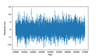
(a)

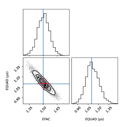
(b)

Figure 1: Timing residuals (panel a) and parameter estimation results (panel b) for the white noise-only simulation (see section 6.1). In panel (b), the blue lines show the injected values, the red point with error bars shows the maximum likelihood estimate obtained using PINT, and the corner plot (black) shows the posterior distribution obtained from the ENTERPRISE analysis.

6.2 EFAC + ECORR

In this simulation, we modify the TOA uncertainties by an EFAC and include an ECORR noise component. Similar to the white noise-only case, we fit the generated TOAs for both timing and noise parameters starting from an initial model with EFAC=1 and ECORR=$10^{-3}$. We explore four versions of this fit, where each noise parameter is allowed to be free or is frozen. The AIC differences for these configurations are listed below:

Configuration	AIC Difference
Free EFAC, Free ECORR	0
Free EFAC, ECORR=0	228
EFAC=1, Free ECORR	331
EFAC=1, ECORR=0	1238

Clearly, both the EFAC and the ECORR are required to model the noise in this dataset. The comparison of the measured EFAC and ECORR values with the injected values is shown in Figure 1, along with the posterior distribution obtained from a Bayesian ENTERPRISE analysis; see Table 4 for the prior distributions used. We see that the maximum likelihood estimates are consistent with the Bayesian estimates within error bars whereas both estimates are slightly offset from the injected values.

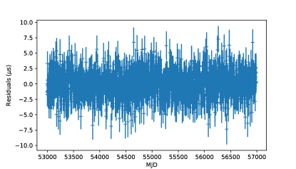
(a)

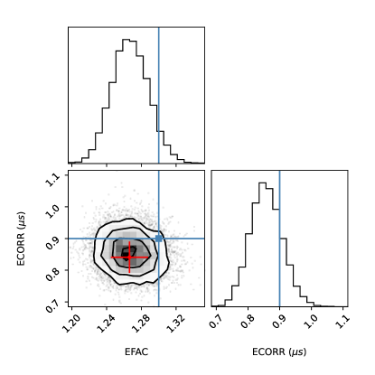
(b)

Figure 2: The timing residuals (panel a) and the parameter estimation results (panel b) for the EFAC + ECORR simulation (see section 6.2). The plotting conventions are identical to Figure 1.

6.3 Achromatic red noise-only

In this simulation, we inject a realization of the achromatic red noise component with a power law spectrum, modeled as a Fourier GP (implemented in PINT as the PLRedNoise model), into the TOAs. We model this noise using the WaveX model, where the component frequencies are taken to be the harmonics of a fundamental frequency $T_{\text{span}}^{-1}$, where $T_{\text{span}}$ is the total observation span. To determine the optimal number of harmonics needed to model the noise, we fit the simulated TOAs using different numbers of harmonics and compute the AIC value corresponding to each case. These AIC values are plotted in Figure 3(a), and the optimum number of harmonics turns out to be 17 (the injected value is 30, see Table 3). The maximum-likelihood estimates for the Fourier coefficients $\hat{a}_{i}$ and $\hat{b}_{i}$ are plotted in the top panel of Figure 3(c), along with its power spectrum in the bottom panel. In Figure 3(c), we see an outlier in the frequency bin containing 1 yr^-1. This can be attributed to the covariance of these Fourier coefficients with the source coordinates, which enter the timing model primarily via the solar system Rømer delay, with a frequency of 1 yr^-1. We fit a power law to the estimated Fourier coefficients as described in section 4.3, estimating the power law amplitude and the spectral index. The best-fit power is also shown in the bottom panel of Figure 3(c), along with its Bayesian counterpart obtained using ENTERPRISE as well as the injected power law spectrum for comparison. Further comparison of these spectral parameter estimates are shown in Figure 3(d), where the posterior distribution obtained from the ENTERPRISE analysis and the injected values are also plotted.

We see that the maximum-likelihood estimates for the red noise spectral parameters differ from the Bayesian estimates only at the $2\sigma$ level. This difference can be attributed to the significant differences in the methods used to obtain these results, as discussed in section 4.3.

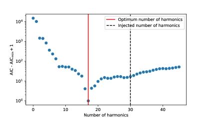
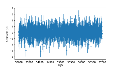
(a)	(b)
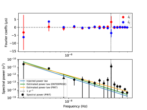
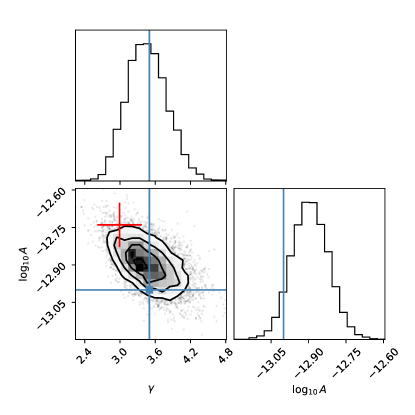
(c)	(d)

Figure 3: Panel (a) shows the $\text{AIC}-\text{AIC}_{\min}+1$ values for the different number of harmonics for the red noise-only simulation (see section 6.3). A red vertical line indicates the optimum number of harmonics. The injected value is indicated by a black dashed vertical line. The Y axis is plotted in a log scale for better visibility (the +1 term is added to $\text{AIC}-\text{AIC}_{\min}$ to enable this). Panel (b) shows the post-fit timing residuals. Panel (c) shows the parameter estimation results. The top sub-panel shows the maximum likelihood estimates of the Fourier sine (blue points) and cosine (red points) coefficients $\hat{a}_{j}$ and $\hat{b}_{j}$ appearing in equation (24). The bottom panel shows the corresponding spectral powers (black points) and the power law fit thereof (orange line) obtained by maximizing the likelihood function given in equation (26). For comparison, the bottom panel also shows the injected power law spectrum (blue line) and the power law spectrum estimated using ENTERPRISE in a Bayesian way (green line). The black dotted line corresponds to 1 yr^-1. Panel (d) shows the comparison of the power law spectral parameters obtained using PINT and ENTERPRISE. The plotting conventions here are identical to Figure 1.

6.4 DM noise-only

In this simulation, we inject a realization of the DM noise with a power law spectrum, modeled as a Fourier GP (implemented in PINT as the PLDMNoise model), into the TOAs. We model this noise using the DMWaveX model, where the component frequencies are taken to be harmonics of $T_{\text{span}}^{-1}$. We begin by determining the optimal number of harmonics using AIC, and the AIC differences for different numbers of harmonics are plotted in Figure 4(a). The optimal number of harmonics turns out to be 22 (the injected value is 30). Figure 4(c) shows the estimated Fourier coefficients in the top panel and the estimated spectral powers, the injected power law spectrum, and the estimated power law spectra (both using PINT and ENTERPRISE) in the bottom panel. The corresponding power law amplitude and spectral index estimates are plotted in Figure 4(d). We see that the power spectrum estimated using PINT and enterprise are consistent with each other as well as with the injected values within the uncertainty levels.

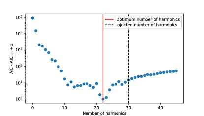
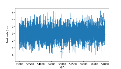
(a)	(b)
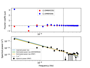
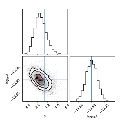
(c)	(d)

Figure 4: Panel (a) shows the $\text{AIC}-\text{AIC}_{\min}+1$ values for the different number of harmonics for the DM noise-only simulation (see section 6.4). The plotting conventions are identical to Figure 3(a). Panel (b) shows the post-fit timing residuals. Panel (c) shows the parameter estimation results. The plotting conventions are identical to Figure 3(c). The error bars in the top sub-panel are too small to be visible. Panel (d) shows the comparison of the power law spectral parameters obtained using PINT and ENTERPRISE. The plotting conventions here are identical to Figure 1.

7 Application to PSR B1855+09

We now proceed to demonstrate and test our methods on the NANOGrav 9-year (NG9) narrowband dataset of PSR B1855+09. This dataset contains 4005 TOAs taken using the Arecibo telescope during 2004–2013 (Arzoumanian et al., 2015). It was chosen because it is distributed as an example dataset together with the PINT source code.

We used the ‘par’ file from the NG9 dataset as a starting point for our analysis after removing the DMX parameters representing piecewise-constant DM variations. We begin our analysis by fitting the timing model parameters, including

1. Astrometric parameters (sky location, proper motion, and parallax)

2. Dispersion measure and its time derivatives (up to the second derivative)

3. Pulsar binary parameters for the BinaryDD model (binary period and period derivative, projected semi-major axis of the pulsar orbit, eccentricity, argument of periapsis, epoch of periapsis passage, companion mass, and orbital sine-inclination.)

4. Frequency-dependent profile evolution parameters (up to third order)

5. Pulsar rotational frequency and its derivative

6. Phase jump between different receivers (430 and L-wide)

7. Overall phase offset

Thereafter, we included the DMWaveX model with 20 harmonics to model the DM variations along with EFAC, EQUAD, and ECORR parameters for each observing system (receiver-backend combinations, denoted as 430_ASP, 430_PUPPI, L-wide_ASP, and L-wide_PUPPI). We have used $T_{\text{span}}^{-1}$ as the fundamental frequency of the DMWaveX components. With this choice, the lower-frequency DM variations will be absorbed into the DM derivatives mentioned above. Note that we did not find any evidence for achromatic red noise in this dataset, likely due to its short time span.

We then used the AIC to determine which noise parameters are truly necessary for the given dataset as demonstrated in subsections 6.1 and 6.2, and it turned out that EQUAD parameters were not needed for 430_ASP and 430_PUPPI. This was verified using the Savage-Dickey ratio (Dickey, 1971) for these parameters, obtained from a Bayesian analysis performed using ENTERPRISE and PTMCMCSampler. Similarly, the optimal number of DMWaveX harmonics was determined to be 10 using the AIC similar to subsection 6.4, and this is shown in Figure 5(a).

Finally, we performed a maximum-likelihood fit using the optimal model. The spectral parameters of the DM noise were estimated following subsection 4.3. The post-fit timing residuals are plotted in 5(b), and the maximum-likelihood DM noise parameter estimates are plotted in 5(c). Figure 5(d) shows a comparison between the maximum-likelihood noise parameter estimates and their Bayesian counterparts (see Table 4 for the prior distributions used) using a corner plot. These plots show that the frequentist and Bayesian estimates agree with each other within their respective uncertainties.

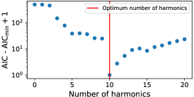
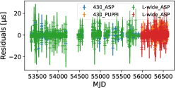
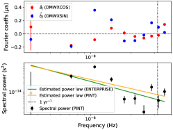
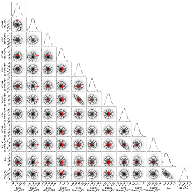
(a) (b) (c) (d)

Figure 5: Parameter estimation results for the NG9 dataset of PSR B1855+09 (see section 7). Panel (a) shows the $\text{AIC}-\text{AIC}_{\min}+1$ values for the different number of DM noise harmonics with identical plotting conventions to Figure 3(a). Panel (b) shows the post-fit timing residuals. The different colors in this panel represent different receiver-backend combinations. Panel (c) shows the parameter estimation results for the DM noise, with identical plotting conventions to Figure 3(c). Panel (d) shows the comparison of the noise parameters obtained using PINT and ENTERPRISE, with identical plotting conventions as Figure 1. Note that the EQUAD and ECORR parameters have units of $\mu$s.

8 New features in PINT

In this section, we briefly summarize the new features that have been implemented in PINT since the publication of Luo et al. (2021). The new timing model components and new fitting methods were discussed in Sections 2.2 and 3–4 respectively, and are not included here.

8.1 Timing model comparison and conversion utilities

Different timing models can be compared with each other using the TimingModel.compare() function. This functionality is also available via the compare_parfiles command line utility.

The convert_binary() function in the pint.binaryconvert module allows the user to convert between different binary models (see Table LABEL:tab:model-components). This functionality can also be accessed via the convert_parfile command line utility. convert_parfile also allows the user to convert between different ‘par’ file formats.

PINT only supports the TDB timescale internally unlike the tempo2 package, which supports both TDB and TCB timescales (Hobbs et al., 2006). However, PINT can now read ‘par’ files in the TCB timescale and convert them to TDB automatically. This conversion can also be performed using the tcb2tdb command line utility.

8.2 Global repository for clock files

Since the TOAs are usually measured against local observatory clocks, a series of clock corrections must be applied to bring them to the TDB timescale (see Luo et al. (2021) for details). These clock corrections are usually distributed as ‘clock files’ containing their deviation from an international time standard (usually UTC(GPS)) over time. PINT now accesses these files from a central repository maintained by the International Pulsar Timing Array consortium (Verbiest et al., 2016). This allows PINT to retain access to the most up-to-date clock corrections without the user having to manually update the clock files.

8.3 TOA simulations

PINT’s simulation functionality is implemented in the pint.simulation module, and can be invoked using the zima command line utility. This module now provides a wide range of functionality on top of simple TOA generation, including the simulation of wideband TOAs, simulation of white noise incorporating EFACs and EQUADs, simulation of different types of single-pulsar correlated noise including ECORR, achromatic red noise, and DM noise, etc. Note that this module can only simulate single-pulsar signals, and it cannot simulate signals that are correlated across pulsars such as the gravitational wave background.

8.4 Bayesian interface

The BayesianTiming class in the pint.bayesian module can be used to perform Bayesian parameter estimation and model selection for pulsar timing datasets. This interface can be used to evaluate the likelihood function, prior distribution, and the prior transform function, and is compatible with both MCMC and nested samplers. This interface supports Bayesian inference on both narrowband and wideband datasets and allows the user to estimate the timing model and white noise parameters. However, estimating correlated noise parameters (in their GP representation) is not yet supported.

8.5 Chi-squared grids

In some cases, rather than determine the best-fit values of all parameters, it is desirable to fit for all but a few parameters while stepping over a grid of a subset of the parameters. This is commonly done with post-Keplerian binary parameters (Damour & Deruelle, 1986) that can constrain the pulsar and companion masses (e.g., Cromartie et al., 2020; Fonseca et al., 2021), since these parameters are often only marginally significant and give overlapping constraints on the masses.

To facilitate this, we have implemented within the pint.gridutils module a number of methods. These enable the $\chi^{2}$ to be computed over grids of intrinsic parameters (such as Shapiro delay companion mass and range) or derived parameters created from combinations of intrinsic parameters (such as characteristic age). The individual model fits are done with the help of the concurrent.futures module (de Groot, 2020) that enables asynchronously launching and tracking multiple jobs and has extensions like clusterfutures that enable deployment on high-performance computing clusters with batch scheduling using slurm (Yoo et al., 2003).

8.6 Publication output

The publish() function in the pint.output.publish module can be used to generate a LaTeX table summary of a dataset comprising a timing model and a set of TOAs. The same functionality is also available through the pintpublish command line utility.

9 Summary and Discussion

In this paper, we describe the new developments in the PINT pulsar timing package, with a focus on frequentist parameter estimation methods. This includes the newly implemented timing model components (Table LABEL:tab:model-components), fitting algorithms (Table 2), and features for performing specific tasks such as simulation, Bayesian inference, etc (Section 8). In particular, we described the Downhill fitter algorithm, an improved version of the linear fitting algorithm commonly used in pulsar timing that is robust against significant non-linearity in the likelihood function as well as regions of the parameter space where the likelihood function is ill-defined.

We presented a new framework within the PINT pulsar timing package to perform frequentist pulsar timing noise characterization, involving the maximum-likelihood estimation of both uncorrelated and correlated noise parameters simultaneously with timing model parameters, as well as a model comparison functionality using the AIC. We demonstrated our parameter estimation and model comparison methods using simulated datasets as well as the NG9 dataset of PSR B1855+09. The results obtained from these exercises show good agreement between our methods and conventional Bayesian methods, indicating the reliability of our methods. Additionally, we also present other new features of PINT, such as new timing model components, timing model comparison & conversion utilities, a global repository for clock files, TOA simulation, an interface for Bayesian analysis, chi-squared grids, and a publication output utility.

The new noise characterization framework should improve the task of pulsar timing in two ways. In pulsar timing projects where Bayesian analysis is deemed not worth the cost, noise characterization is either not done at all or is only done in an ad hoc manner. In such projects, our new framework can provide a convenient and inexpensive alternative for noise characterization, ensuring more robust timing solutions. In high-precision applications where Bayesian noise characterization is necessary, our framework can help accelerate the data preparation/combination stage by integrating noise characterization into interactive pulsar timing workflows and pulsar timing pipelines without needing a Bayesian analysis step. The quick parameter estimates and model comparisons provided by our framework can quicken the iterative refinement of noise models. Further, the frequentist noise parameter estimates can act as independent cross-checks for Bayesian results and as starting points for MCMC samplers to help them converge faster.

Appendix A System and frequency-dependent delays

The phenomenological model used to account for frequency-profile evolution is given by

$$\Delta_{\text{FD}}=\sum_{p}\mathfrak{F}_{p}\left[\log\left(\frac{\nu}{\text{1 GHz}}\right)\right]^{p}\,,$$ (A1)

where $p$ is an index and $\mathfrak{F}_{p}$ is known as an FD parameter. In large data sets containing TOAs obtained using many different observing systems, it is often insufficient to model the frequency-dependent profile evolution using global FD parameters that affect all TOAs. The need for system-dependent FD parameters can arise due to (a) the data reduction procedures used for different observing systems being different, (b) different template profiles being used to compute TOAs for different systems, etc. The system-dependent FD delay is given by

$$\Delta_{\text{FDJump}}=\sum_{pq}\mathfrak{F}_{pq}\left[\log\left(\frac{\nu}{\text{1 GHz}}\right)\right]^{p}\mathcal{M}_{q}\,,$$ (A2)

where $\mathfrak{F}_{pq}$ is known as a system-dependent FD parameter (also known as an FD jump), and $\mathcal{M}_{q}$ is a TOA selection mask. An alternative model for $\Delta_{\text{FDJump}}$, originally implemented in tempo2, is also available:

$$\Delta_{\text{FDJump}}=\sum_{pq}\mathfrak{F}_{pq}\left(\frac{\nu}{\text{1 GHz}}\right)^{p}\mathcal{M}_{q}\,.$$ (A3)

The two expressions above can be toggled using a Boolean parameter FDJUMPLOG.

References

- Agazie et al. (2023) Agazie, G., Antoniadis, J., Anumarlapudi, A., et al. 2023, arXiv e-prints, arXiv:2309.00693, doi: 10.48550/arXiv.2309.00693
- Agazie et al. (2023a) Agazie, G., Anumarlapudi, A., Archibald, A. M., et al. 2023a, The Astrophysical Journal Letters, 951, L10, doi: 10.3847/2041-8213/acda88
- Agazie et al. (2023b) —. 2023b, The Astrophysical Journal Letters, 952, L37, doi: 10.3847/2041-8213/ace18b
- Alam et al. (2021) Alam, M. F., Arzoumanian, Z., Baker, P. T., et al. 2021, The Astrophysical Journal Supplement Series, 252, 5, doi: 10.3847/1538-4365/abc6a1
- Antoniadis et al. (2023) Antoniadis, J., Arumugam, P., Arumugam, S., et al. 2023, Astronomy & Astrophysics, 678, A50, doi: 10.1051/0004-6361/202346844
- Arzoumanian et al. (2015) Arzoumanian, Z., Brazier, A., Burke-Spolaor, S., et al. 2015, The Astrophysical Journal, 813, 65, doi: 10.1088/0004-637X/813/1/65
- Ashton et al. (2022) Ashton, G., Bernstein, N., Buchner, J., et al. 2022, Nature Reviews Methods Primers, 2, 39, doi: 10.1038/s43586-022-00121-x
- Backer & Hellings (1986) Backer, D. C., & Hellings, R. W. 1986, Annual Review of Astronomy and Astrophysics, 24, 537, doi: 10.1146/annurev.aa.24.090186.002541
- Blandford & Teukolsky (1976) Blandford, R., & Teukolsky, S. A. 1976, The Astrophysical Journal, 205, 580, doi: 10.1086/154315
- Burnham & Anderson (2004) Burnham, K. P., & Anderson, D. R. 2004, Sociological Methods & Research, 33, 261, doi: 10.1177/0049124104268644
- Caballero et al. (2018) Caballero, R. N., Guo, Y. J., Lee, K. J., et al. 2018, Monthly Notices of the Royal Astronomical Society, 481, 5501, doi: 10.1093/mnras/sty2632
- Coles et al. (2011) Coles, W., Hobbs, G., Champion, D. J., Manchester, R. N., & Verbiest, J. P. W. 2011, Monthly Notices of the Royal Astronomical Society, 418, 561, doi: 10.1111/j.1365-2966.2011.19505.x
- Cromartie et al. (2020) Cromartie, H. T., Fonseca, E., Ransom, S. M., et al. 2020, Nature Astronomy, 4, 72, doi: 10.1038/s41550-019-0880-2
- Damour & Deruelle (1986) Damour, T., & Deruelle, N. 1986, Annales de L’Institut Henri Poincare Section (A) Physique Theorique, 44, 263
- Damour & Taylor (1992) Damour, T., & Taylor, J. H. 1992, Physical Review D, 45, 1840, doi: 10.1103/PhysRevD.45.1840
- Davis et al. (1985) Davis, J. L., Herring, T. A., Shapiro, I. I., Rogers, A. E. E., & Elgered, G. 1985, Radio Science, 20, 1593, doi: 10.1029/RS020i006p01593
- de Groot (2020) de Groot, C. 2020, The Concurrent.Futures Library (Apress), 12, doi: 10.1007/978-1-4842-6582-6_12
- Demorest et al. (2012) Demorest, P. B., Ferdman, R. D., Gonzalez, M. E., et al. 2012, The Astrophysical Journal, 762, 94, doi: 10.1088/0004-637X/762/2/94
- Deng et al. (2012) Deng, X. P., Coles, W. A., Hobbs, G. B., et al. 2012, Monthly Notices of the Royal Astronomical Society, 424, 244. https://api.semanticscholar.org/CorpusID:118614238
- Dickey (1971) Dickey, J. M. 1971, The Annals of Mathematical Statistics, 42, 204 , doi: 10.1214/aoms/1177693507
- Donner et al. (2020) Donner, J. Y., Verbiest, J. P. W., Tiburzi, C., et al. 2020, Astronomy & Astrophysics, 644, A153, doi: 10.1051/0004-6361/202039517
- Edwards et al. (2006) Edwards, R. T., Hobbs, G. B., & Manchester, R. N. 2006, Monthly Notices of the Royal Astronomical Society, 372, 1549, doi: 10.1111/j.1365-2966.2006.10870.x
- Fiore et al. (2023) Fiore, W., Levin, L., McLaughlin, M. A., et al. 2023, The Astrophysical Journal, 956, 40, doi: 10.3847/1538-4357/aceef7
- Fonseca et al. (2021) Fonseca, E., Cromartie, H. T., Pennucci, T. T., et al. 2021, The Astrophysical Journal Letters, 915, L12, doi: 10.3847/2041-8213/ac03b8
- Foreman-Mackey (2016) Foreman-Mackey, D. 2016, The Journal of Open Source Software, 1, 24, doi: 10.21105/joss.00024
- Foreman-Mackey et al. (2013) Foreman-Mackey, D., Hogg, D. W., Lang, D., & Goodman, J. 2013, Publications of the Astronomical Society of the Pacific, 125, 306, doi: 10.1086/670067
- Foster & Backer (1990) Foster, R. S., & Backer, D. C. 1990, The Astrophysical Journal, 361, 300, doi: 10.1086/169195
- Freire & Wex (2010) Freire, P. C. C., & Wex, N. 2010, Monthly Notices of the Royal Astronomical Society, 409, 199, doi: 10.1111/j.1365-2966.2010.17319.x
- Harris et al. (2020) Harris, C. R., Millman, K. J., van der Walt, S. J., et al. 2020, Nature, 585, 357, doi: 10.1038/s41586-020-2649-2
- Hazboun et al. (2022) Hazboun, J. S., Simon, J., Madison, D. R., et al. 2022, The Astrophysical Journal, 929, 39, doi: 10.3847/1538-4357/ac5829
- Hee et al. (2015) Hee, S., Handley, W. J., Hobson, M. P., & Lasenby, A. N. 2015, Monthly Notices of the Royal Astronomical Society, 455, 2461, doi: 10.1093/mnras/stv2217
- Hobbs (2014) Hobbs, G. 2014, TEMPO2 examples. https://www.jb.man.ac.uk/~pulsar/Resources/tempo2_examples_ver1.pdf
- Hobbs et al. (2019) Hobbs, G., Guo, L., Caballero, R. N., et al. 2019, Monthly Notices of the Royal Astronomical Society, 491, 5951, doi: 10.1093/mnras/stz3071
- Hobbs et al. (2006) Hobbs, G. B., Edwards, R. T., & Manchester, R. N. 2006, Monthly Notices of the Royal Astronomical Society, 369, 655, doi: 10.1111/j.1365-2966.2006.10302.x
- Hotan et al. (2004) Hotan, A. W., van Straten, W., & Manchester, R. N. 2004, Publications of the Astronomical Society of Australia, 21, 302, doi: 10.1071/AS04022
- Hunter (2007) Hunter, J. D. 2007, Computing in Science & Engineering, 9, 90, doi: 10.1109/MCSE.2007.55
- Johnson et al. (2023) Johnson, A. D., Meyers, P. M., Baker, P. T., et al. 2023, arXiv e-prints, arXiv:2306.16223, doi: 10.48550/arXiv.2306.16223
- Jones & Qin (2022) Jones, G. L., & Qin, Q. 2022, Annual Review of Statistics and Its Application, 9, 557, doi: 10.1146/annurev-statistics-040220-090158
- Kopeikin (1995) Kopeikin, S. M. 1995, The Astrophysical Journal Letters, 439, L5, doi: 10.1086/187731
- Kopeikin (1996) —. 1996, The Astrophysical Journal Letters, 467, L93, doi: 10.1086/310201
- Kramer et al. (2006) Kramer, M., Stairs, I. H., Manchester, R. N., et al. 2006, Science, 314, 97, doi: 10.1126/science.1132305
- Kramer et al. (2021) Kramer, M., Stairs, I. H., Manchester, R. N., et al. 2021, Physical Review X, 11, 041050, doi: 10.1103/PhysRevX.11.041050
- Laal et al. (2023) Laal, N., Lamb, W. G., Romano, J. D., et al. 2023, Physical Review D, 108, 063008, doi: 10.1103/PhysRevD.108.063008
- Lange et al. (2001) Lange, C., Camilo, F., Wex, N., et al. 2001, Monthly Notices of the Royal Astronomical Society, 326, 274, doi: 10.1046/j.1365-8711.2001.04606.x
- Lentati et al. (2014) Lentati, L., Alexander, P., Hobson, M. P., et al. 2014, Monthly Notices of the Royal Astronomical Society, 437, 3004, doi: 10.1093/mnras/stt2122
- Lorimer & Kramer (2012) Lorimer, D. R., & Kramer, M. 2012, Handbook of Pulsar Astronomy (Cambridge University Press)
- Luo et al. (2021) Luo, J., Ransom, S., Demorest, P., et al. 2021, The Astrophysical Journal, 911, 45, doi: 10.3847/1538-4357/abe62f
- Madison et al. (2019) Madison, D. R., Cordes, J. M., Arzoumanian, Z., et al. 2019, The Astrophysical Journal, 872, 150, doi: 10.3847/1538-4357/ab01fd
- Manchester (2017) Manchester, R. N. 2017, Journal of Astrophysics and Astronomy, 38, 42, doi: 10.1007/s12036-017-9469-2
- Nice et al. (2015) Nice, D., Demorest, P., Stairs, I., et al. 2015, Tempo: Pulsar timing data analysis, Astrophysics Source Code Library, record ascl:1509.002. http://ascl.net/1509.002
- Niell (1996) Niell, A. E. 1996, Journal of Geophysical Research, 101, 3227, doi: 10.1029/95JB03048
- Park et al. (2021) Park, R. S., Folkner, W. M., Williams, J. G., & Boggs, D. H. 2021, The Astronomical Journal, 161, 105, doi: 10.3847/1538-3881/abd414
- Pennucci (2019) Pennucci, T. T. 2019, The Astrophysical Journal, 871, 34, doi: 10.3847/1538-4357/aaf6ef
- Pennucci et al. (2014) Pennucci, T. T., Demorest, P. B., & Ransom, S. M. 2014, The Astrophysical Journal, 790, 93, doi: 10.1088/0004-637X/790/2/93
- Powell (1964) Powell, M. J. D. 1964, The Computer Journal, 7, 155, doi: 10.1093/comjnl/7.2.155
- Price-Whelan et al. (2022) Price-Whelan, A. M., Lim, P. L., Earl, N., et al. 2022, The Astrophysical Journal, 935, 167, doi: 10.3847/1538-4357/ac7c74
- Rafikov & Lai (2006) Rafikov, R. R., & Lai, D. 2006, Physical Review D, 73, 063003, doi: 10.1103/PhysRevD.73.063003
- Ransom (2001) Ransom, S. M. 2001, PhD thesis, Harvard University, Massachusetts
- Reardon et al. (2023) Reardon, D. J., Zic, A., Shannon, R. M., et al. 2023, The Astrophysical Journal Letters, 951, L6, doi: 10.3847/2041-8213/acdd02
- Sazhin (1978) Sazhin, M. V. 1978, Soviet Astronomy, 22, 36
- Shapiro (1964) Shapiro, I. I. 1964, Phys. Rev. Lett., 13, 789, doi: 10.1103/PhysRevLett.13.789
- Susobhanan et al. (2018) Susobhanan, A., Gopakumar, A., Joshi, B. C., & Kumar, R. 2018, Monthly Notices of the Royal Astronomical Society, 480, 5260, doi: 10.1093/mnras/sty2177
- Taylor (1992) Taylor, J. H. 1992, Philosophical Transactions of the Royal Society of London. Series A: Physical and Engineering Sciences, 341, 117, doi: 10.1098/rsta.1992.0088
- Taylor & Weisberg (1989) Taylor, J. H., & Weisberg, J. M. 1989, The Astrophysical Journal, 345, 434, doi: 10.1086/167917
- Tiburzi et al. (2021) Tiburzi, C., Shaifullah, G. M., Bassa, C. G., et al. 2021, Astronomy & Astrophysics, 647, A84, doi: 10.1051/0004-6361/202039846
- Vallisneri (2020) Vallisneri, M. 2020, libstempo: Python wrapper for Tempo2, Astrophysics Source Code Library, record ascl:2002.017. http://ascl.net/2002.017
- Vallisneri et al. (2020) Vallisneri, M., Taylor, S. R., Simon, J., et al. 2020, The Astrophysical Journal, 893, 112, doi: 10.3847/1538-4357/ab7b67
- van Haasteren & Vallisneri (2014) van Haasteren, R., & Vallisneri, M. 2014, Monthly Notices of the Royal Astronomical Society, 446, 1170, doi: 10.1093/mnras/stu2157
- van Haasteren & Vallisneri (2014) van Haasteren, R., & Vallisneri, M. 2014, Physical Review D, 90, 104012, doi: 10.1103/PhysRevD.90.104012
- van Straten & Bailes (2011) van Straten, W., & Bailes, M. 2011, Publications of the Astronomical Society of Australia, 28, 1–14, doi: 10.1071/AS10021
- Verbiest et al. (2016) Verbiest, J. P. W., Lentati, L., Hobbs, G., et al. 2016, Monthly Notices of the Royal Astronomical Society, 458, 1267, doi: 10.1093/mnras/stw347
- Virtanen et al. (2020) Virtanen, P., Gommers, R., Oliphant, T. E., et al. 2020, Nature Methods, 17, 261, doi: 10.1038/s41592-019-0686-2
- Weisberg & Huang (2016) Weisberg, J. M., & Huang, Y. 2016, The Astrophysical Journal, 829, 55, doi: 10.3847/0004-637X/829/1/55
- Wolszczan & Frail (1992) Wolszczan, A., & Frail, D. A. 1992, Nature, 355, 145, doi: 10.1038/355145a0
- Xu et al. (2023) Xu, H., Chen, S., Guo, Y., et al. 2023, Research in Astronomy and Astrophysics, 23, 075024, doi: 10.1088/1674-4527/acdfa5
- Yoo et al. (2003) Yoo, A. B., Jette, M. A., & Grondona, M. 2003, in Job Scheduling Strategies for Parallel Processing, ed. D. Feitelson, L. Rudolph, & U. Schwiegelshohn (Berlin, Heidelberg: Springer Berlin Heidelberg), 44–60
- You et al. (2012) You, X. P., Coles, W. A., Hobbs, G. B., & Manchester, R. N. 2012, Monthly Notices of the Royal Astronomical Society, 422, 1160, doi: 10.1111/j.1365-2966.2012.20688.x
- You et al. (2007) You, X. P., Hobbs, G. B., Coles, W. A., Manchester, R. N., & Han, J. L. 2007, The Astrophysical Journal, 671, 907, doi: 10.1086/522227
- Zhu et al. (2018) Zhu, W. W., Desvignes, G., Wex, N., et al. 2018, Monthly Notices of the Royal Astronomical Society, 482, 3249, doi: 10.1093/mnras/sty2905