Convex optimization on CAT(0) cubical complexes
Abstract
We consider geodesically convex optimization problems involving distances to a finite set of points in a CAT(0) cubical complex. Examples include the minimum enclosing ball problem, the weighted mean and median problems, and the feasibility and projection problems for intersecting balls with centers in . We propose a decomposition approach relying on standard Euclidean cutting plane algorithms. The cutting planes are readily derivable from efficient algorithms for computing geodesics in the complex.
Key words: convex, cutting plane, geodesic, CAT(0), cubical complex
AMS Subject Classification: 90C48, 52A41, 57Z25, 65K05
1 Introduction: optimization in Hadamard space
Metric spaces in which points can always be joined by geodesics — isometric images of real intervals — support a wide variety of interesting convex optimization problems [31, 4]. Convex optimization is best understood in Hadamard spaces: complete geodesic spaces satisfying the CAT(0) inequality, which requires that squared-distance functions to given points are all 1-strongly convex. Manifolds comprise the most familiar examples, including Hilbert space, hyperbolic space, and the space of positive-definite matrices with its affine-invariant metric.
From a computational perspective, in the special case of manifolds, gradient-based methods are available [8]. On the other hand, even with no differentiable structure, some Hadamard spaces allow efficient computation of geodesics. Particularly interesting are phylogenetic tree spaces [7] and more general CAT(0) cubical complexes [2]. In these spaces, geodesics can be computed in polynomial time [26, 16]. Along with phylogenetic models, applications include reconfigurable systems in robotics [1, 12].
Unfortunately, optimization algorithms in the setting of a general Hadamard space are scarce and slow. Methods based on alternating projections are sometimes available [5], but other general-purpose algorithms typically rely on some predetermined sequence of step sizes. The quintessential example is the problem of computing the mean of a finite set in the geodesic space , which is the unique minimizer of the function
| (1.1) |
To compute the mean, the only known general methods iteratively update the th iterate to a point on the geodesic between and some point , chosen randomly [28] or via some deterministic strategy [17, 6, 22]: a standard example is
To compute the mean of the set by this method, for example, starting at the point and using , results in the slowly converging sequence . Computation in practice confirms this slow convergence: see [24] for experiments in the manifold of positive definite matrices, and [10] for experiments in phylogenetic tree space.
In this work, we focus on the particular case of geodesically convex optimization on a CAT(0) cubical complex. This setting has several features suggesting faster algorithmic possibilities. First, as we have noted, computing geodesics is tractable. Secondly, the underlying space, by definition, decomposes into Euclidean cubes. Lastly, restricted to each cube, geodesically convex optimization problems reduce to standard Euclidean convex optimization. Using these ingredients, we suggest a new cutting plane approach. Our central technique uses geodesics in CAT(0) cubical complexes to derive Euclidean subgradients of distance functions restricted to individual cells in the complex. We illustrate the new algorithm on a simple computational example.
2 CAT(0) cubical complexes
We begin with some standard definitions [9]. Let be a metric space. A geodesic path is a distance-preserving mapping . The image is called a geodesic segment. We say that is a (uniquely) geodesic space if every two points in are joined by a (unique) geodesic segment. A function is convex when its composition with every geodesic path is convex.
Given three points in a geodesic space, a geodesic triangle is the union of three geodesic segments (its sides) joining each pair of points. A comparison triangle for is a triangle in that has side lengths equal to those of . A geodesic metric space is called CAT(0) if in every geodesic triangle, distances between points on its sides are no larger than corresponding distances in a comparison triangle. CAT(0) spaces are uniquely geodesic. A Hadamard space is a complete CAT(0) space. For any nonempty closed convex subset of a Hadamard space , every point in has a unique nearest point in .
Let and be two nonconstant geodesics paths in a CAT(0) space issuing at the same point . For and , denote and , and let be a comparison triangle for . Then the angle is a nondecreasing function of both and , and the Alexandrov angle between and is defined by
A polyhedral cell is a geodesic metric space isometric to the convex hull of finitely many points in a Euclidean space : we usually identify and . By a face of , we mean a nonempty set that is either itself, or is the intersection of with a hyperplane such that belongs to one of the closed half-spaces determined by . The dimension of a face is the dimension of the intersection of all affine subspaces containing it. The -dimensional faces of a cell are called its vertices, and the -dimensional faces are called its edges. A polyhedral complex is a set of polyhedral cells of various dimensions such that the face of any cell is also a cell of the complex, and the intersection of any two cells is either empty or a face of both. The complex is finite if it consists of finitely many cells, and is cubical if each -dimensional cell is isometric to the unit cube .
Given two points in a polyhedral complex , the distance is the infimum of lengths of piecewise geodesic paths joining to . A piecewise geodesic path from to is an ordered sets of points in such that for every , there exists a cell with ; its length is . If is connected and finite, then is a complete geodesic metric space.
In what follows, we will, in general, consider finite cubical complexes. As proved by Gromov [14], a cubical complex is CAT(0) if and only if it is simply connected and satisfies the following “link” condition at each vertex. Consider the edges containing that vertex. Any set of distinct such edges, each pair of which is contained in a common 2-dimensional cell, must consist of edges all contained in a common -dimensional cell. For more discussion, see [16].
Example 2.1 (A simple CAT(0) cubical complex)
Consider the space
with the distance induced by the Euclidean metric: in other words, the distance between points is the Euclidean length of the shortest path between them in . This space is a finite CAT(0) cubical complex, consisting of the three -dimensional cells
More generally than the example above, any simply connected subcomplex of , the integer lattice cubing of , is CAT(0), because no three edges containing a vertex can, pairwise, be edges of common squares, so the link condition holds. On the other hand, consider the cubical complex formed from the cube in by taking just the three faces containing zero. This simply connected cubical complex is not CAT(0) because it fails the link condition: the edges connecting zero with the three standard unit vectors are pairwise contained in common squares, but no cell contains all three.
3 Decomposition
Before describing a decomposition approach to convex optimization on cubical complexes, we first illustrate by considering the mean of three points in the simple space of Example 2.1.
Example 3.1 (A simple mean calculation)
In the CAT(0) cubical complex described in Example 2.1, consider the set consisting of the standard unit vectors and , along with . To compute the mean of , we must solve the underlying optimization problem (1.1). To do so, we decompose into the union of three cells , , and , and solve the restricted problem over each cell in turn:
Worth noting is that the first and third problems are not smooth. The optimal solution of both the second and third problems is the point . However, the optimal solution of the first problem is the strictly better point , where . This point is therefore the mean.
This example illustrates a significant feature of mean calculations in cubical complexes or other Hadamard spaces that are not manifolds. Even when we can compute geodesics efficiently, that tool alone does not immediately allow us to recognize whether or not a given point is the mean, let alone compute the mean. For example, along the geodesics between the point and each point in the set , the objective defined by equation (1.1) is minimized at . However, is not the mean: it does not minimize over the whole space .
Returning to our general problem, we can minimize a convex function over a finite cubical complex by minimizing over each of the finitely many cells comprising separately. To each of these subproblems we can apply a standard algorithm for Euclidean convex minimization. Rather than exhaustively optimizing over every cube, we can instead consider the following conceptual method, inspired by a somewhat analogous conceptual approach sketched in [25, Algorithm 4.4].
Algorithm 3.2 (Minimize convex on cubical complex )
While unnecessary formally, we would naturally always choose a maximal cell , meaning that no strictly larger cell contains .
Proposition 3.3 (Termination)
For any finite cubical complex and any convex function , Algorithm 3.2 terminates, returning a minimizer of .
Proof The procedure terminates, since the space is a finite complex. Throughout the procedure, at the current iterate , the value never increases. At termination, therefore minimizes the objective over every cell containing . Since is convex, therefore minimizes it over the whole space .
As an example, consider the simple example above, on the space (2.1). In Algorithm 3.2, as soon as we choose the cube , the procedure terminates with the iterate equal to the mean, whether or not or have already been searched.
Means in metric trees
It is illuminating to consider the behavior of Algorithm 3.2 for computing means for the simplest class of CAT(0) cubical complex: the case when the space is a finite metric tree. In that case, consists of the edges and vertices of a finite connected acyclic graph, where we identify edges with 1-dimensional cells of unit length, intersecting at common 0-dimensional cells — the vertices. The Gromov link condition holds trivially.
We consider the problem of computing the mean of a finite subset of finite metric tree. We illustrate with the following example [18, Example 1], which is a special case of the “open books” [18] discussed in Appendix A.
Example 3.4 (Stickiness)
The 3-spider is the finite metric tree consisting of three copies of the interval joined at the shared origin . Denote the three copies , and consider a set consisting of three points satisfying
(One particular example is for each .) A quick calculation shows that the mean is the shared origin . Unlike in the Euclidean case, the mean is insensitive to small changes in the points : it is sticky in the sense of [18].
Consider a general finite metric tree , with vertex set and edge set . Via a finite computation, we can exactly compute the mean of a finite subset using Algorithm 3.2 to minimize the function in equation (1.1). The data of the problem, in addition to the graph , consists, for each point , of an endpoint of an edge containing , and the distance between and along the edge .
Problems of this kind have been widely studied in the operations research literature, in the context of facility location problems [15]. More typical than the mean problem in that context are the “median” or “minimax” problems, involving the sum or maximum of the distance functions rather than sum of their squares, although [15, Section 3.4] notes an efficient algorithm for the mean problem due to Goldman. Goldman’s 1972 algorithm [13] for the “1-center problem on a tree network”, in the terminology of [29], involves a “trichotomy” at each iteration: after checking an edge the algorithm stops or is confined to one of the two subtrees resulting from deleting that edge.
Algorithm 3.2, it transpires, has the same trichotomy property. At the outset of each iteration, we have a current vertex , and a current set of already optimized edges. For each point , we first find the unique sequence of edges joining to : its cardinality is the distance . The distance from to is therefore given by
We next choose a vertex neighboring the vertex and with corresponding edge outside the set , terminating if there is no such edge. We then minimize over . Denote the set of those points for which by . If we identify with the unit interval , where corresponds to the point 0 and corresponds to the point 1, then for any point on , we have
We now find the unique point minimizing the strictly convex function
The unconstrained minimizer is
If , then the algorithm terminates: the mean is the point on at a distance from . Otherwise, we update to include , update the current iterate to if , and repeat.
Solving the subproblems
In the case of mean computations for metric trees, Algorithm 3.2 involves one-dimensional subproblems with closed-form solutions. In general, however, the subproblems are multivariate, requiring iterative techniques.
The approach outlined in [25, Algorithm 4.4] for computing means in the phylogenetic tree space of [7] relies on a smooth but nonconvex interior-penalty philosophy, the complexity of which is unclear. By contrast, our approach via Algorithm 3.2 generates subproblems that, while nonsmooth, are convex. At each iteration of Algorithm 3.2 we can identify the cell isometrically with a cube , for some dimension , and then apply a linearly convergent Euclidean cutting plane algorithm, efficient in theory and reliable in practice.
One such cutting plane approach for general convex objectives would be to apply the randomized method of [19], which needs just evaluations of to approximately solve the minimization problem over the cube . More precisely, if , then with constant probability the excess is reduced to after no more than function evaluations. In essence, the method is subgradient-based: at each iteration, it approximates a subgradient, using function evaluations.
In this work, however, we are primarily interested in structured functions composed simply from distance functions: a typical example is the mean objective in equation (1.1). Our central observation is that such objectives support methods based on explicit subgradients, an approach with three potential advantages. First, we arrive at a deterministic rather than randomized algorithm. Secondly, the complexity of the available algorithms is better: the classical ellipsoid method still requires function evaluations, but more recent cutting plane algorithms improve this to [30]. Lastly, we can experiment with algorithms known to be effective in practice, like proximal or level bundle methods [20].
4 Subgradients of distance functions
In a CAT(0) cubical complex , the geodesic between any two points, and , is computable in polynomial time [2]. Suppose that lies in a cell , and consider the distance function to , restricted to . We next show how to use the geodesic to calculate a subgradient of this function at the point .
We start with a simple tool.
Lemma 4.1
Let be a CAT(0) space and consider three points with and . Then
Proof From the triangle inequality we know
We deduce
and hence
Consequently we have
where the second inequality follows from the law of cosines.
Theorem 4.2
In a CAT(0) cubical complex , consider two cells and with a common face , and points and . Denote the nearest point to in by . Then is also the nearest point to in . Furthermore, for any point , if and , then the following angle inequality holds:
| (4.3) |
Before proving the theorem, it helps to keep in mind a simple example.
Example 4.4
Consider any cubical subcomplex of containing the cells
Their common face is the cell
Consider the two points
The closest point to in , in either the Euclidean distance or the distance it induces in , is
At , the angle between the nontrivial geodesic and any nontrivial geodesic with is minimized (either in or in ) when . In fact, the stronger inequality (4.3) holds.
Proof of Theorem 4.2. The result only involves geodesics with endpoints in and . All such geodesics lie in the interval between and , in the terminology of [2], so without loss of generality we can suppose by [2, Theorem 3.5] that is a subcomplex of , the integer lattice cubing of .
Without loss of generality, we can suppose that and are unit cubes in that are contained in and both contain . Corresponding to any two partitions of the index set into disjoint subsets,
we can define such cubes in using the relationship set by
We lose no generality in assuming that and are of this form. To illustrate, Example 4.4 corresponds to the partitions
The point lies in the common face , which is the cube in defined by
Since we deduce
It is easy to compute componentwise the Euclidean nearest point to the point in the cube : since , for each we have
Since , we deduce
for the index set
Clearly we have , and hence the line segment is contained in . That line segment is therefore also a geodesic in . Since distances between points in are no less than their Euclidean distance, we deduce .
Since and , those line segments are also geodesics in . The distance in between pairs of points, one on each line segment, is never less than the Euclidean distance, so in , the angle between those geodesics is never less than their Euclidean angle. Moreover, since the points , , and all lie in the cube , and the points , , and all lie in the cube , the angles and in equal the corresponding Euclidean angles. Thus, it is enough to prove (4.3) for Euclidean angles, and hence, in what follows, we consider all angles to be Euclidean.
Since , the formula above for shows . Consequently we deduce and
Applying the law of cosines, we get
and
Thus,
where the last inequality follows because is the Euclidean nearest point to in and .
Consider any distinct points and in a CAT(0) cubical complex . The CAT(0) property ensures that the distance function to , denoted by is a convex function on [4, Example 2.2.4]. Using the algorithm of [2], we can compute the geodesic : it passes via a sequence of nontrivial geodesics
through some corresponding connected sequence of cells (neither sequence being necessarily unique). We refer to as an initial segment and to as a corresponding initial cell.
Given a cube , a vector is a subgradient of a convex function at a point if
The subdifferential is just the set of such subgradients.
We can now derive our central tool, which allows us to compute subgradients of distance functions restricted to cells in cubical complexes.
Theorem 4.5 (Subgradients of distance functions)
Consider a cube and a point . Suppose that is a cell in a CAT(0) cubical complex , and consider any point . Let denote the restriction of the distance function to . If then . Suppose, on the other hand, that . In the geodesic , let be an initial segment corresponding to an initial cell . Denote by the common face of and . In any ambient Euclidean space for , denote the nearest point to in by . If , then . On the other hand, if , then
Proof The case is trivial, so assume henceforth . By definition, we have .
Consider first the case . In that case, by Theorem 4.2, is the nearest point to in , and since , we deduce that is also the nearest point to in (see [9, Proposition II.2.4]), so follows.
On the other hand, consider the case . We must prove
This inequality holds when . When , we have
To illustrate the result, we consider a simple example.
Example 4.6 (Calculating a subgradient of a distance function)
Consider the CAT(0) cubical complex the cells of which are the following squares in , along with their edges and vertices:
For the point , the distance function is given by
This function must be convex on , so in particular it is convex on . Differentiating shows that, for points in the interior of the set , regarded as a subset of , we have
The two cases in this formula describe a set of full measure around the point , and as approaches within this set, the gradient has a unique limit: . Standard properties of Euclidean convex functions therefore show that the function restricted to has Gateaux derivative at . The Euclidean normal cone to at is , so we deduce
| (4.7) |
We now compare this with the subgradient provided by Theorem 4.5. Let denote the point . The geodesic from to consists of the two line segments in the square and in the square . The common face of and is , and in the square , the nearest point to in the face is the point . The unit vector in the direction is therefore . The angle has cosine , so the theorem asserts that the vector is a subgradient of at . This is confirmed by equation (4.7).
5 Means, medians, and circumcenters
In any metric space , we can consider a variety of interesting optimization problems associated with a given nonempty finite set , posed simply in terms of the distance functions to points . Foremost among these are weighted mean problems, which entail minimizing functions defined by
| (5.1) |
for some given weights , for , and a given exponent . The special case is known as the median problem. Another well-known example is the minimum enclosing ball or circumcenter problem, which entails minimizing over the function
When the space is a finite CAT(0) cubical complex, we can solve weighted mean and minimum enclosing ball problems using Algorithm 3.2 and Theorem 4.5. Consider first the weighted mean problem [4, Example 6.3.4]. The function (5.1) is convex, and a minimizer always exists, by [4, Lemma 2.2.19]. For , the function is strictly convex, so the minimizer is unique. In the case , minimizers may not be unique.
To compute means and medians in general Hadamard spaces, the only methods previously analyzed appear to be the splitting proximal point algorithms described in [6]. As we noted in the introduction, such methods are inevitably slow. In the case of a finite CAT(0) cubical complex, we instead propose Algorithm 3.2 as a faster alternative.
To implement Algorithm 3.2, we first fix attention on some cell in the complex . Via an isometric embedding, we make the identification . Using the notation of Theorem 4.5, we seek to minimize the convex function
For this purpose, we can use a standard Euclidean cutting plane method, of the kind described in [11, Chapter 2]. Such methods require a separation/subgradient oracle of the following form. Consider any input point .
-
•
If , then output a hyperplane separating from .
-
•
Otherwise, return the value and a subgradient .
Theorem 4.5 allows us to implement this oracle. Separating any point from is trivial. On the other hand, for any point in , for each point , the theorem describes how to calculate a corresponding subgradient . We deduce , and then adding gives a subgradient:
Example 5.2 (A simple mean calculation, concluded)
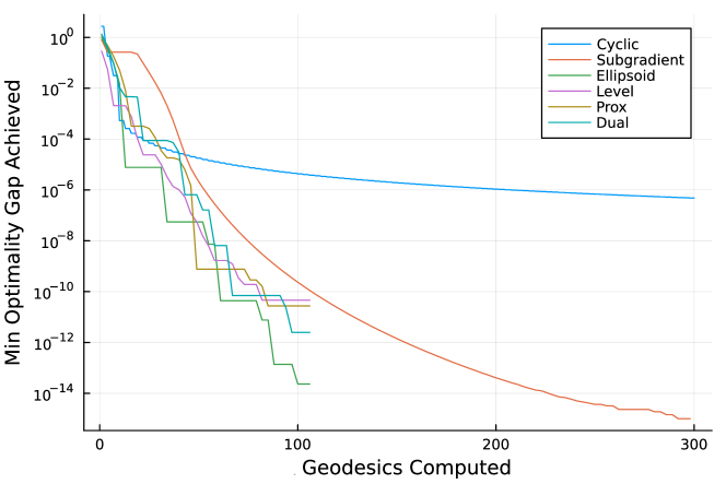
We return to the simple mean problem in Examples 2.1 and 3.1. On each of the three cells we solve the corresponding subproblem using a standard subgradient-based method, deploying the subgradients available through Theorem 4.5. We compare six methods: four cutting plane methods, the classical subgradient method, and the cyclic proximal point method from [6]. The cutting plane methods consist of the classical ellipsoid algorithm and three standard bundle methods from [20]: a level bundle method, a proximal bundle method, and a dual level method. The methods all converge to the optimal solution of each subproblem: the true mean in the cell , and the point in the other two cells. The behavior of the objective value in the case of the cell is shown in Figure 1, plotted against the number of geodesics computed: the behavior in the other cells is similar. Even on this small low-dimensional example, the cyclic proximal point method is relatively slow. The subgradient method, although clearly sublinear, converges reasonably quickly on this example, in part because the objective function happens to be smooth around the optimal solution. The cutting plane methods are all faster, and the plot suggests the linear convergence we expect.
Turning to the minimum enclosing ball problem [4, Example 2.2.18], we can frame the problem as minimizing the strongly convex function defined by
The unique solution is called the circumcenter of . Previous literature makes no apparent reference to algorithms for the minimum enclosing ball problem in general Hadamard spaces. A subgradient-style method has been proposed recently in [21], with the slow convergence rate typical of subgradient methods. In the case of CAT(0) cubical complexes, we again propose Algorithm 3.2 as a faster alternative.
We follow the same approach, focusing on some cell and minimizing the strongly convex function defined by
To compute a subgradient of at a point , we first select, from the set , a point at maximum distance from . We then appeal to Theorem 4.5 to calculate a corresponding subgradient . Standard Euclidean subgradient calculus [27] now gives us the desired subgradient: .
To apply Algorithm 3.2 to a mean, median, or circumcenter problem, having implemented the separation/subgradient oracle, we next choose a cutting plane method to solve the subproblems over cells . Most classically — albeit not the best choice in theory or practice, as discussed in the introduction — we could apply the ellipsoid algorithm, starting with the smallest Euclidean ball containing . That algorithm converges linearly: by [11, Theorem 2.4], if the cell has dimension , then after calls to the oracle, we find an iterate in at which the value of exceeds by no more than
If is in fact strongly convex (as in the case of the mean or circumcenter problems), then the iterates also converge linearly, to the unique minimizer of on .
6 The distance to an intersection of balls
In addition to mean and circumcenter problems, another fundamental problem associated with a given nonempty finite subset of a metric space , and posed simply in terms of distance functions, is the intersecting balls problem. Centered at each point , given a radius , we consider the closed ball . We seek a point in their intersection:
In any Hadamard space , we could approach the intersecting balls problem via the method of cyclic projections [5, 3]: the projection of any point onto a ball centered at is easy to compute from the geodesic , since the projection must lie on the geodesic. However, in a general Hadamard space, the rate at which the method converges to a point in the intersection is not clear, and when the intersection is empty, the behavior of the iterates is not well understood [23].
When the space is a finite CAT(0) cubical complex, we take a different approach to the intersecting balls problem, again using Algorithm 3.2 and Theorem 4.5. Consider the related problem of minimizing over the objective function
Since this function is coercive, it has a minimizer, by [4, Lemma 2.2.19]. Consider any such minimizer . If , then we have solved our problem, and on the other hand, if , then the set must be empty. We therefore seek to minimize the function defined by
We follow the same strategy as for the mean problem in the previous section, focusing on individual cells in the complex , making the identification and seeking to minimize the convex function defined by
As before, to implement a cutting plane algorithm, we need to find a subgradient of at any input point . To that end, for each point , we compute the distances , and calculate a vector as follows. If , then we define . On the other hand, if , then we appeal to Theorem 4.5 to calculate a subgradient . In that way, standard Euclidean subgradient calculus [27] guarantees that is a subgradient of the convex function given by
from which we deduce our desired subgradient:
We can now apply a cutting plane algorithm.
Refining the intersecting balls problem, we might seek to compute the distance from a given point to the intersection of balls . We can approach this problem by a bisection search strategy. We first run the previous algorithm, either finding a point or detecting that none exists, in which case we terminate. If we find , we begin our bisection search, always maintaining an interval containing the distance from to . Initially we set and . At each iteration, we consider the midpoint of the current interval, and apply the previous algorithm to the intersecting balls problem . If the intersection is empty, we update ; otherwise we update . We then repeat.
References
- [1] A. Abrams and R. Ghrist. State complexes for metamorphic robots. The International Journal of Robotics Research, 23:811–826, 2004.
- [2] F. Ardila, M. Owen, and S. Sullivant. Geodesics in CAT(0) cubical complexes. Advances in Applied Mathematics, 48:142–163, 2012.
- [3] D. Ariza-Ruiz, G. López-Acedo, and A. Nicolae. The asymptotic behavior of the composition of firmly nonexpansive mappings. J. Optim. Theory Appl., 167:409–429, 2015.
- [4] M. Bac̆ák. Convex Analysis and Optimization in Hadamard Spaces. De Gruyter, Berlin, 2014.
- [5] M. Bac̆ák, I. Searston, and B. Sims. Alternating projections in CAT(0) spaces. J. Math. Anal. Appl., 385:599–607, 2012.
- [6] M. Bačák. Computing medians and means in Hadamard spaces. SIAM Journal on Optimization, 24:1542–1566, 2014.
- [7] L.J. Billera, S.P. Holmes, and K. Vogtmann. Geometry of the space of phylogenetic trees. Advances in Applied Mathematics, 27:733–767, 2001.
- [8] N. Boumal. An Introduction to Optimization on Smooth Manifolds. Cambridge University Press, Cambridge, 2023.
- [9] M.R. Bridson and A. Haefliger. Metric Spaces of Non-Positive Curvature. Springer-Verlag, Berlin, 1999.
- [10] D.G. Brown and M. Owen. Mean and variance of phylogenetic trees. Systematic Biology, 69:139–154, 2020.
- [11] S. Bubeck. Convex optimization: algorithms and complexity. Foundations and Trends® in Machine Learning, 8(3-4):231–357, 2015.
- [12] R. Ghrist and V. Peterson. The geometry and topology of reconfiguration. Advances in Applied Mathematics, 38:302–323, 2007.
- [13] A.J. Goldman. Minimax location of a facillity in a network. Transportation Science, 6:407–418, 1972.
- [14] M. Gromov. Structures métriques pour les variétés Riemanniennes, volume 1 of Textes Mathématiques. CEDIC, Paris, Edited by J. Lafontaine and P. Pansu, 1981.
- [15] P. Hansen, M. Labbé, D. Peeters, and J.-F. Thisse. Single facility location on networks. Annals of Discrete Mathematics, 31(113-146), 1987.
- [16] K. Hayashi. A polynomial time algorithm to compute geodesics in CAT(0) cubical complexes. Discrete and Computational Geometry, 65:636–654, 2021.
- [17] J. Holbrook. No dice: a deterministic approach to the Cartan centroid. Journal of the Ramanujan Mathematical Society, 27:509–521, 2012.
- [18] T. Holz, S. Huckemann, Huiling Le, J.S. Marron, J.C. Mattingly, E. Miller, J. Nolen, M. Owen, V. Patrangenaru, and S. Skwerer. Sticky central limit theorems on open books. Annals of Applied Probability, 23:2238–2258, 2013.
- [19] Yin Tat Lee, A. Sidford, and S.S. Vempala. Efficient convex optimization with membership oracles. Proceedings of Machine Learning Research, 75:1–3, 2018 arXiv:1706.07357.
- [20] C. Lemaréchal, A. Nemirovskii, and Y. Nesterov. New variants of bundle methods. Math. Programming, 69(1, Ser. B):111–147, 1995. Nondifferentiable and large-scale optimization (Geneva, 1992).
- [21] A.S. Lewis, G. López-Acedo, and A. Nicolae. Horoballs and the subgradient method. arXiv:2403.15749, 2024.
- [22] Yongdo Lim and M. Palfia. Weighted deterministic walks for the least squares mean on Hadamard spaces. Bulletin of the London Mathematical Society, 46:561–570, 2014.
- [23] A. Lytchak and A. Petrunin. Cyclic projections in Hadamard spaces. J. Optim. Theory Appl., 194:636–642, 2022.
- [24] E.M. Massart, J.M. Hendrickx, and P.-A. Absil. Matrix geometric means based on shuffled inductive sequences. Linear Algebra and its Applications, 542:334–359, 2018.
- [25] E. Miller, M. Owen, and J.S. Provan. Polyhedral computational geometry for averaging metric phylogenetic trees. Advances in Applied Mathematics, 68:51–91, 2015.
- [26] M. Owen and S. Provan. A fast algorithm for computing geodesic distances in tree space. IEEE/ACM Transactions on Computational Biology and Bioinformatics, 8:2–13, 2011.
- [27] R.T. Rockafellar. Convex analysis. Princeton Mathematical Series, No. 28. Princeton University Press, Princeton, N.J., 1970.
- [28] K.-T. Sturm. Nonlinear martingale theory for processes with values in metric spaces of nonpositive curvature. Ann. Probab., 30:1195–1222, 2002.
- [29] B.C. Tansel, R.L. Francis, and T.J. Lowe. State of the art — location on networks: a survey. Part I: the p-center and p-median problems. Management Science, 29:482–497, 1983.
- [30] P.M. Vaidya. A new algorithm for minimizing convex functions over convex sets. Mathematical Programming, 73:291–341, 1996.
- [31] Hongyi Zhang and S. Sra. First-order methods for geodesically convex optimization. Journal of Machine Learning Research, 49:1–22, 2016.
Appendix A Appendix: core cells
An interesting source of illustrative computational examples arises from the class of cubical complexes consisting of a collection of cells all sharing one common face. As observed in [18], although this face is lower-dimensional than it often contains the mean of a set of points distributed throughout .
Example A.1 (An open book [18])
Consider three copies of the square joined along the shared edge : the “spine” of the open book. Denote the three copies , and consider any points satisfying
(An example is for each .) A quick calculation shows that the mean is the following point on the spine:
The spine is thus sticky: the mean remains there for all small perturbations of the three points.
Definition A.2
In a cubical complex, if all distinct pairs of maximal cells have the same nonempty intersection , then we call the core.
The core, if it exists, is a common face of all the maximal cells. For example, the 3-spider has the core . The maximal cells may not all have the same dimension. For example, the complex consisting of the maximal cells in
has core .
Proposition A.3
Any cubical complex with a core is CAT(0).
Proof Consider a cubical complex with a core . The cells of consist just of all the faces of maximal cells. Since is contractible to any point in , it is simply connected.
We next observe that Gromov’s link condition holds. To see this, given any vertex, consider any finite set of incident edges, each pair of which lie in a common -dimensional cell of . For each maximal cell , let denote those edges in that lie in but not in the common face . Consider any two maximal cells . Suppose that there exist edges and . Any -dimensional cell containing both and must be a face of some maximal cell . The edge lies in both and , but by assumption not in , so in fact . But the same argument shows , giving a contradiction. We deduce that either or , proving that the collection of sets for maximal cells is totally ordered by inclusion. The collection therefore has maximal element, for some maximal cell . Every edge in lies in this cell , and hence in some -dimensional face of , as required.
We next compute geodesics.
Proposition A.4
Consider points and in a cubical complex with a core . If some cell contains both points, then the geodesic is the line segment joining them in that cell. On the other hand, if no cell contains both, then there are maximal cells and such that and . In , consider the distance between and , its orthogonal projection onto . Analogously, in , consider the distance between and , its orthogonal projection onto . Consider the following convex combination in :
Then the geodesic is the union of the two geodesics and .
Proof Note that the geodesic must pass through the face , so it is the union of two geodesics and for some point . The length of this path is
As varies over , this function is convex, and viewed on any ambient Euclidean space in which lives, its gradient is
| (1.5) |
Notice
so
and hence the first term in the expression (1.5), when , becomes
By symmetry, the second term is identical, after multiplying by . Hence the gradient (1.5) is zero when , so indeed minimizes the length.