Novel Local Characteristic Decomposition Based Path-Conservative Central-Upwind Schemes
Abstract
We introduce local characteristic decomposition based path-conservative central-upwind schemes for (nonconservative) hyperbolic systems of balance laws. The proposed schemes are made to be well-balanced via a flux globalization approach, in which source terms are incorporated into the fluxes: This helps to enforce the well-balanced property when the resulting quasi-conservative system is solved using the local characteristic decomposition based central-upwind scheme recently introduced in [A. Chertock, S. Chu, M. Herty, A. Kurganov, and M. Lukáčová-Medvid’ová, J. Comput. Phys., 473 (2023), Paper No. 111718]. Nonconservative product terms are also incorporated into the global fluxes using a path-conservative technique. We illustrate the performance of the developed schemes by applying them to one- and two-dimensional compressible multifluid systems and thermal rotating shallow water equations.
Key words: Local characteristic decomposition, path-conservative central-upwind schemes, flux globalization, compressible multifluids, thermal rotating shallow water equations.
AMS subject classification: 76M12, 65M08, 35L65, 86-08, 76T99.
1 Introduction
This paper is focused on the development of highly accurate and robust numerical methods for the nonconservative hyperbolic systems of balance laws, which in the one-dimensional (1-D) case read as
| (1.1) |
where is a spatial variable, is the time, is a vector of unknown functions, are nonlinear fluxes, , and are source terms.
Designing a numerical scheme for (1.1) is a challenging task for a number of reasons. First, it is well-known that solutions of (1.1) may develop complicated nonsmooth structures even for smooth initial data. Second, the presence of nonconservative products (when ) brings many challenges for studying these systems both theoretically and numerically. In general, when is discontinuous, weak solutions of (1.1) cannot be understood in the sense of distributions. Instead, one can introduce Borel measure solutions [19, 30, 31]. This concept of weak solutions was utilized to develop path-conservative finite-volume (FV) methods; see, e.g., [35, 6, 7, 8, 36, 38, 1, 9] and reference therein. Third, a novel scheme should be well-balanced (WB) in the sense that it should be capable of exactly preserving some of the physically relevant steady-state solutions satisfying
Here, and is the vector of equilibrium variables, which are constant at the steady states provided is invertible; see [26].
In this paper, we focus on one of the popular classes of FV methods, the Riemann-problem-solver-free central-upwind (CU) schemes, which were originally introduced in [28, 29, 25] as a “black-box” solver for general multidimensional hyperbolic systems of conservation laws and then successfully applied to a variety of hyperbolic systems. In [8], the CU schemes were first reformulated in a path-conservative framework and then extended to the 1-D nonconservative systems (1.1), resulting in the second-order path-conservative CU (PCCU) schemes. These schemes are WB in the sense that they are capable of preserving simple steady-state solutions like “lake-at-rest” of several shallow water models.
In order to design PCCU schemes capable of preserving more complicated steady states, path-conservative techniques were incorporated into the flux globalization framework: This results in a new class of flux globalization based WB PCCU schemes introduced in [26]. A flux globalization approach, which was introduced in [14, 5, 20, 21, 33], relies on the following quasi-conservative form of (1.1):
| (1.2) |
where is a global flux
| (1.3) |
and is an arbitrary number. The flux globalization based WB PCCU schemes are obtained by applying the CU numerical flux to the semi-discretization of (1.2) and by using the path-conservative technique for the evaluation of the integrals in (1.3). These schemes have been applied to a variety of hyperbolic systems in [2, 3, 4, 10, 26, 18].
Even though the flux globalization based WB PCCU schemes from [26] are accurate, efficient, and robust, higher resolution of the numerical solutions can be achieved by reducing numerical dissipation present in those schemes. This can be done, for example, by using the local characteristic decomposition (LCD) based CU (LCD-CU) numerical fluxes instead of the original CU ones employed in [2, 3, 4, 10, 26]. The LCD-CU schemes have been recently introduced in [12] for hyperbolic systems of conservation laws and we use the same LCD based framework to enhance the performance of the flux globalization based WB PCCU schemes. The proposed scheme combines for the first time the modifications enhancing the performance of the CU schemes for both conservative and nonconservative hyperbolic systems in multiple space dimensions. We derive the new LCD-PCCU schemes and apply them to two particular systems. First, we consider the -based compressible multifluid systems, which can be, in principle, written in the conservative form, but we use its nonconservative formulation to achieve high resolution of material interfaces. Second, we consider a challenging thermal rotating shallow water (TRSW) model, which contains geometric source term due to a nonflat bottom topography, source terms due to Coriolis forces, and generically nonconservative momentum exchange terms.
The rest of the paper is organized as follows. In §2, we briefly describe the 1-D second-order LCD-CU scheme. In §3, we propose the novel scheme by considering the nonconservative system (1.1) and design a 1-D flux globalization based WB LCD-PCCU scheme. In §4, we extend the 1-D LCD-PCCU scheme to the two-dimensional (2-D) case. Finally, in §5, we apply the developed LCD-PCCU schemes to the -based compressible multifluid systems and TRSW equations. We illustrate the performance of the scheme on a number of numerical examples.
2 1-D LCD-CU Scheme
In this section, we briefly describe the second-order semi-discrete LCD-CU scheme, which is a slightly modified version of the scheme from [12]. For the difference between the schemes, we refer the reader to Remarks 2.1–2.3 below.
We consider a 1-D hyperbolic system of conservative laws
| (2.1) |
cover the computational domain with the uniform cells of size centered at , and denote by the computed cell averages of ,
which are assumed to be available at a certain time . Note that both and many other indexed quantities below are time-dependent, but from here on, we suppress their time-dependence for the sake of brevity.
The computed cell averages (2.1) are evolved in time by numerically solving the following system of ODEs:
where the LCD-CU numerical fluxes are given by
| (2.2) |
Here, and are the one-sided values of a piecewise linear interpolant
| (2.3) |
at the cell interface , namely
| (2.4) |
In order to ensure the non-oscillatory nature of this reconstruction, we compute the slopes in (2.4) using a generalized minmod limiter [32, 34, 40]:
| (2.5) |
applied in the component-wise manner. Here, the minmod function is defined as
| (2.6) |
and the parameter can be used to control the amount of numerical viscosity present in the resulting scheme. We have taken in all of the numerical experiments reported in §5.
The diagonal matrices , , and are given by
| (2.7) | ||||
with
| (2.8) | |||
where
Here, is the Jacobian and the matrices and are such that is diagonal, where and is either a simple average or another type of average of the and states. The one-sided local speeds of propagation can be estimated using the largest and the smallest eigenvalues of , for example, by taking
Finally, in (2.8) is a very small desingularization constant, which is taken in all of the numerical examples reported in §5.
Remark 2.1
Remark 2.2
We perform a piecewise linear reconstruction for the conservative variables rather than the local characteristic variables as it was done in [12]. As no substantial spurious oscillations have been observed in any of the conducted numerical examples, there is no need to switch to the local characteristic variables in this case. This allows the developed scheme to be more efficient than the original LCD-CU scheme from [12].
3 1-D Flux Globalization Based LCD-PCCU Scheme
In this section, we propose an extension of the LCD-CU scheme from §2 to the nonconservative system (1.1) and design a 1-D flux globalization based LCD-PCCU scheme.
We apply the LCD-CU scheme to the quasi-conservative system (1.2)–(1.3) to obtain
| (3.1) |
where the numerical fluxes are given by (compare with (2.2))
| (3.2) |
Here, are the global fluxes, which are computed as the same as in [3, §2].
The global fluxes are computed using the point values , which, in order to ensure the WB property of the resulting scheme, are to be obtained with the help of a piecewise linear reconstruction (2.3)–(2.6) applied to the equilibrium variables (instead of ):
where . We then obtain the corresponding values by solving the (nonlinear systems of) equations
| (3.3) |
for and , respectively. We emphasize that the values cannot be used in (3.2) instead of as may not be equal to at discrete steady states. We therefore use another set of point values , which are obtained by solving modified versions of (3.3):
Here, the functions are the modifications of the functions , which are made in such a way that as long as and, at the same time, and for smooth solutions; see [10, 3, 2, 4, 26] for examples of such modifications.
The diagonal matrices , , and in (3.2) are defined by (2.7)–(2.8), but with
where and the matrices and are such that is diagonal for . Finally, the one-sided local speeds of propagation are estimated by
Remark 3.1
The introduced 1-D semi-discrete flux globalization based LCD-PCCU scheme is WB. In order to prove this, we only need to show that if the discrete data are at a steady state, namely, if , then the RHS of (3.1) vanishes. Following the proof of [3, Theorem 2.1], we obtain
| (3.4) |
Substituting (3.4) and (2.9) into (3.2) and taking into account the fact that at the steady states , yields
which ensures that the RHS of (3.1) vanishes.
4 2-D Flux Globalization Based LCD-PCCU Scheme
In this section, we propose a novel 2-D LCD-PCCU scheme for
| (4.1) |
where , , , and . To this end, we design the 2-D scheme in a “dimension-by-dimension” manner.
As in the 1-D case, we first rewrite the general 2-D nonconservative system (4.1) in the following quasi-conservative form:
| (4.2) |
where
with and being arbitrary numbers.
Applying the 2-D version of the semi-discrete LCD-CU scheme from §2 to the quasi-conservative system (4.2) results in the following system of ODEs:
| (4.3) |
where the numerical fluxes and are given by
| (4.4) | ||||
All of the terms in (4.4) are computed as in §3 separately in the - and -directions.
The global fluxes and are computed using the WB path-conservative technique as in [2]. The LCD matrices , , , , , and are computed as in [12], but based on the eigensystems of and . As in §2, we do not employ local characteristic variables in the piecewise linear reconstruction and perform the desingularization of , , , , , and as in (2.8).
Remark 4.1
The introduced 2-D semi-discrete flux globalization based LCD-PCCU scheme is WB in the sense that it is capable of exactly preserving discrete steady states, for which is independent of and is independent of . We omit the proof for the sake of brevity.
5 Numerical Examples
In this section, we apply the developed LCD-PCCU schemes to the -based compressible multifluid and TRSW equations. We conduct several numerical experiments and compare the performance of the LCD-PCCU schemes with their PCCU counterparts obtained by applying the original CU numerical fluxes in (3.1) and (4.3). For instance, in the 1-D case, such a PCCU scheme is obtained by replacing (2.8) by
In all of the numerical examples, we have solved the ODE systems (3.1) and (4.3) using the three-stage third-order strong stability preserving (SSP) Runge-Kutta method (see, e.g., [23, 22]) and used the CFL number 0.45.
5.1 -Based Compressible Multifluid Equations
In this section, we show the applications of the developed LCD-PCCU schemes introduced in §3 and §4 to the 1-D and 2-D -based compressible multifluid systems [11, 39], which in the 2-D case can be written as (4.1) with , , , , , and . Here, is the density, and are the - and -velocities, is the pressure, and is the total energy. The system is closed through the following (stiff) equation of state (EOS) for each of the fluid components:
| (5.1) |
where the parameters and represent the specific heat ratio and stiffness parameter, respectively (when for all of the components, the system reduces to the ideal gas multicomponent case). The variables and are defined as and .
Remark 5.1
We note that the studied -based compressible multifluid equations contain no source terms and thus there is no need to numerically enforce the WB property. We therefore do not need to introduce any equilibrium variables—instead, we reconstruct the conservative quantities and replace , , and in (3.2) and (4.4) by , , and , respectively.
Remark 5.2
In Appendix A, we provide the expressions for the matrices and and the corresponding matrices and for the 1-D and 2-D -based compressible multifluid systems, respectively. The matrices and can be obtained in an analogous way.
5.1.1 One-Dimensional Examples
In this section, we consider two numerical examples for the 1-D version of the -based compressible multifluid equations.
Example 1—“Shock-Bubble” Interaction
In the first example taken from [17], we consider the “shock-bubble” interaction problem. The initial data are given by
which correspond to a left-moving shock, initially located at , and a resting “bubble” with a radius of 0.25, initially located at the origin.
We impose the solid wall boundary conditions at the both ends of the computational domain and compute the numerical solutions by both the LCD-PCCU and PCCU schemes until the final time on a uniform mesh with . The obtained densities are presented in Figure 5.1 together with the reference solution computed by the PCCU scheme on a much finer mesh with . As one can see, the LCD-PCCU scheme achieves sharper resolution than the PCCU one.
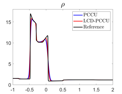
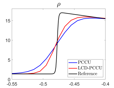
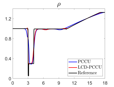
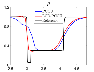
Example 2—Water-Air “Shock-Bubble” Interaction
In the second 1-D example also taken from [17], we consider a gas-liquid multifluid system, where the liquid component is modeled by the stiff EOS (5.1) with . The initial conditions,
correspond to the left-moving shock, initially located at , and a resting air “bubble” with a radius 3, initially located at .
We impose the free boundary conditions at the both ends of the computational domain and compute the numerical solutions until the final time on a uniform mesh with by both the LCD-PCCU and PCCU schemes. The obtained results are presented in Figure 5.2 together with the reference solution computed by the PCCU scheme on a much finer mesh with . As one can see, the LCD-PCCU solution achieves sharper resolution than its PCCU counterpart, especially of the contact wave located at about .
5.1.2 Two-Dimensional Examples
We now consider three 2-D examples, in which we plot the Schlieren images of the magnitude of the density gradient field, . To this end, we use the shading function
where the numerical derivatives of the density are computed using standard central differencing.
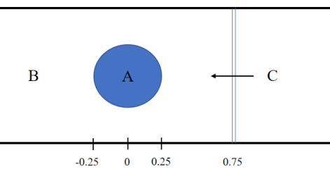
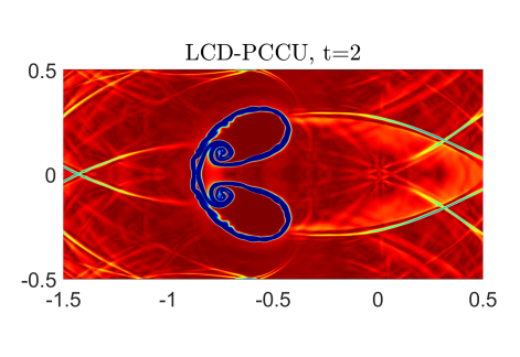
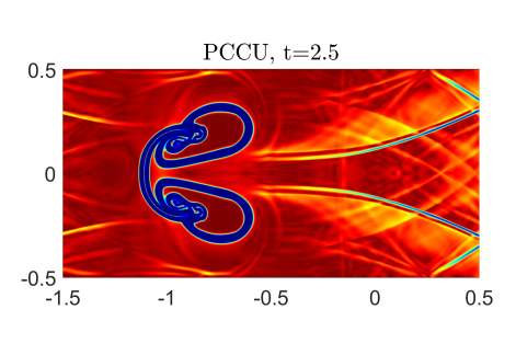
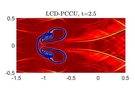
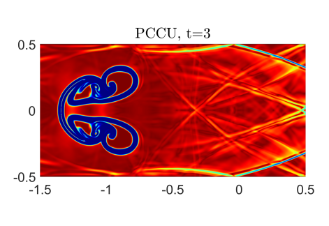
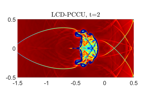
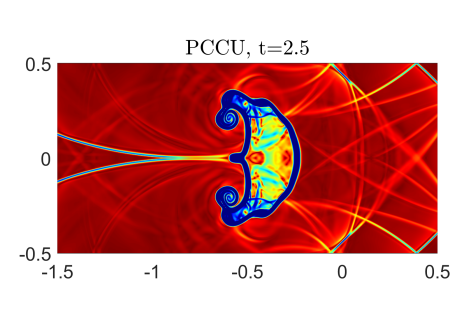
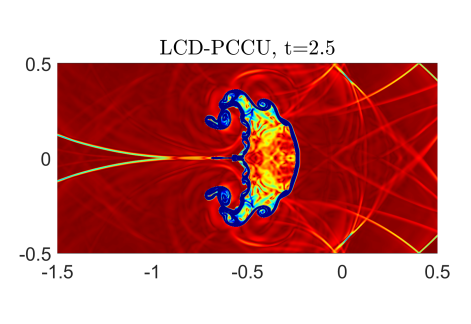
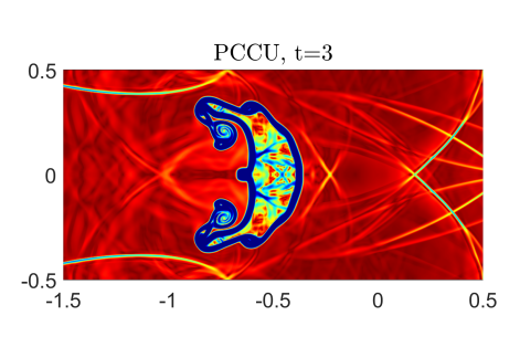
Example 3—Shock-Helium Bubble Interaction
In the first 2-D example taken from [37, 15], a shock wave in the air hits the light resting bubble which contains helium. We take the following initial conditions:
where regions A, B, and C are outlined in Figure 5.3, and the computational domain is . We impose the solid wall boundary conditions on the top and bottom and the free boundary conditions on the left and right edges of the computational domain.
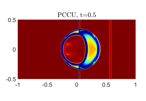
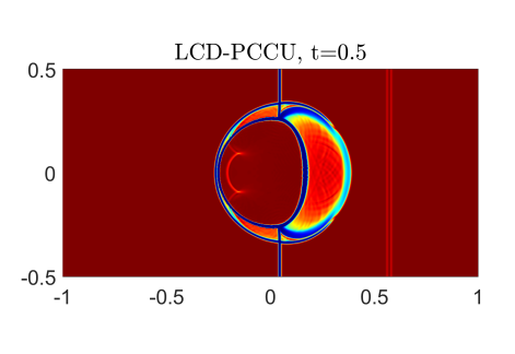
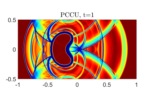
We compute the numerical solutions until the final time on a uniform mesh with . In Figure 5.4, we present different stages of the shock-bubble interaction computed by the PCCU and LCD-PCCU schemes. One can clearly see that the bubble interface develops very complex structures after the bubble is hit by the shock, especially at large times. We note that the obtained results are in a good agreement with the experimental findings presented in [24] and the computational results presented in [37, 15, 13]. Notably, at an early time , the resolution of the bubble interface significantly improves with the implementation of the LCD-PCCU scheme. As time progresses, instabilities arise within the interface, which are smeared by a more dissipative PCCU scheme. The differences in resolution become more pronounced at later times and , and especially at , indicating that the LCD-PCCU scheme clearly outperforms the PCCU one.
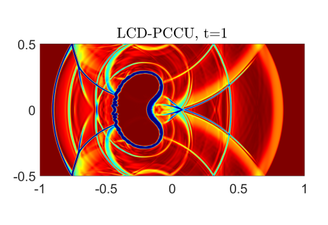
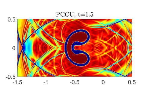
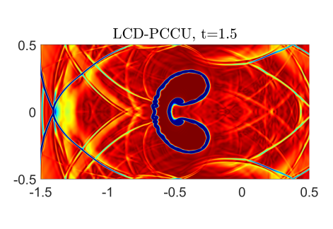
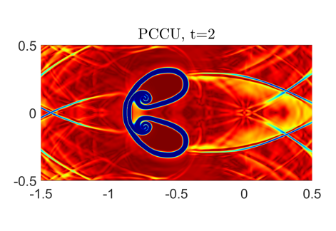
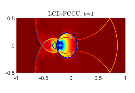
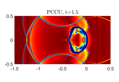
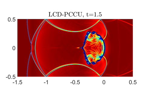
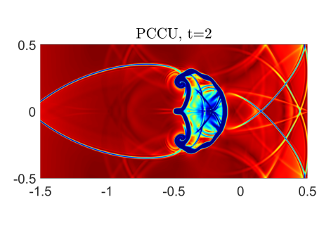
Example 4—Shock-R22 Bubble Interaction
In the second 2-D example also taken from [37, 15], a shock wave in the air hits the heavy resting bubble which contains R22 gas. The initial conditions are
and the rest of the settings are the same as in Example 3.
We compute the numerical solutions until the final time on a uniform mesh with and present different stages of the shock-bubble interaction computed by the PCCU and LCD-PCCU schemes in Figure 5.5. One can clearly see that upon encountering the bubble, the shock wave undergoes both refraction and reflection. Under the force of the shock, the bubble undergoes compression and motion. These findings are in a good agreement with the computational results reported in [37, 15]. Figure 5.5 demonstrates that the LCD-PCCU scheme captures material interfaces more accurately (compared to the PCCU scheme) and also enhances the resolution of fine details of the computed solution. Once again, this indicates that the LCD-PCCU scheme is less diffusive than its PCCU counterpart.
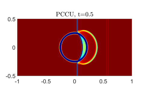
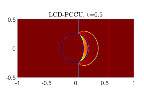
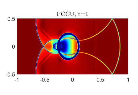
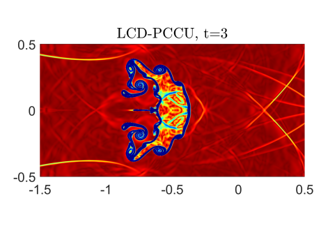
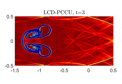
Example 5—A Cylindrical Explosion Problem
In the last 2-D example taken from [17] (see also [41]), we consider the case where a cylindrical explosive source is located between an air-water interface and an impermeable wall. The initial conditions are given by
with the solid wall boundary conditions imposed at the bottom, and the free boundary conditions set on the other sides of the computational domain .
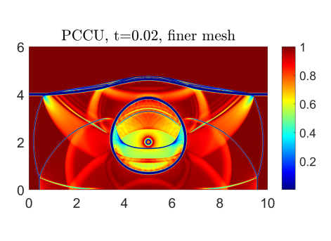
We compute the numerical solutions until the final time on a uniform mesh with by the studied PCCU and LCD-PCCU schemes. In Figure 5.6, we present time snapshots of the obtained results, which qualitatively look similar to the numerical results reported in [17, 41]. As one can see, the LCD-PCCU scheme captures both the material interfaces and many of the developed wave structures substantially sharper than the PCCU scheme.
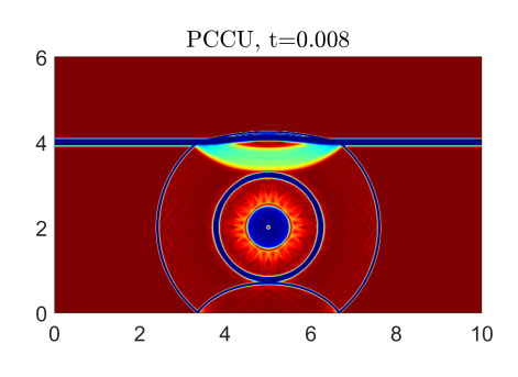
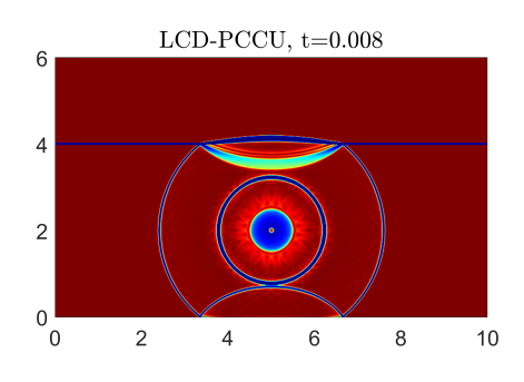
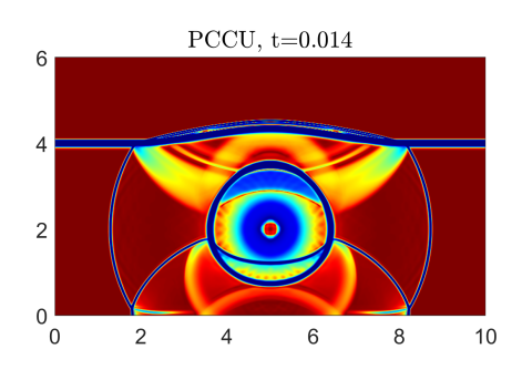
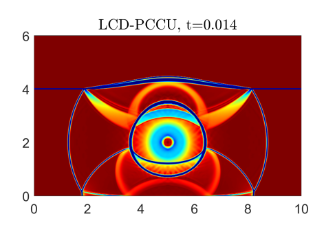
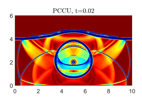
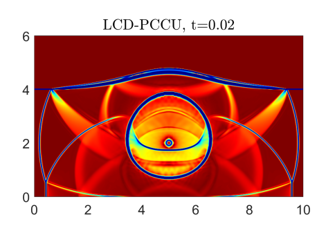
One can also notice a substantial difference between the PCCU and LCD-PCCU solutions at the final time. In order to clarify this point, we refine the mesh and compute the numerical solution on a finer mesh with by the PCCU scheme and present the obtained result in Figure 5.7, where one can clearly see that the PCCU solution computed on a finer mesh is close to the LCD-PCCU solution computed with . Once again, this indicates that the LCD-PCCU solution is more accurate than the PCCU one.
5.2 Thermal Rotating Shallow Water Equations
In this section, we apply the developed LCD-PCCU schemes to the 1-D and 2-D TRSW equations [27], which in the 2-D case can be written as the system (4.1) with
|
|
(5.2) |
where denotes the thickness of the fluid layer, and are the zonal and meridional velocities, and are the corresponding discharges, is the layer-averaged buoyancy variable, and stands for a time-independent bottom topography. In the oceanic context, , where is the acceleration due to gravity, and are the variable and constant parts of the water density, respectively. In the atmospheric context, the densities and should be replaced with the potential temperatures and . Finally, is the Coriolis parameter, where and are positive constants.
Remark 5.3
For the TRSW equations, we use the equilibrium variables introduced in [2] and compute the point values ( and in the 1-D case and , , , and in the 2-D case) as well as the global fluxes ( in the 1-D case and and in the 2-D case) precisely as it was done in [2]. We have also used the same numerical diffusion switch function, which helps to enforce the WB property, as in [2].
Remark 5.4
In Appendix B, we provide the expressions for the matrices and and the corresponding matrices and for the 1-D and 2-D TRSW equations, respectively. The matrices and can be obtained in an analogous way.
5.2.1 One-Dimensional Examples
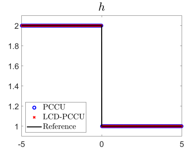
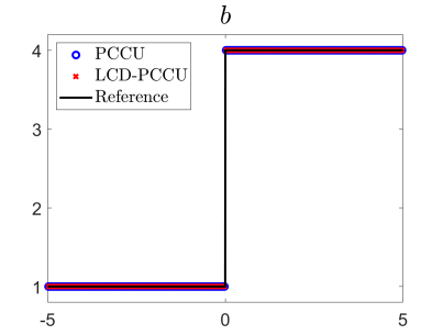
Example 6—Constant Pressure Equilibrium
In the first example taken from [2], we consider the following initial data:
| (5.3) |
which are prescribed in the computational domain together with the flat bottom topography subject to the free boundary conditions.
We first compute the numerical solution by the PCCU and LCD-PCCU schemes until the final time on the uniform mesh with and plot the obtained fluid thickness and buoyancy variables in Figure 5.8, where the reference solution is computed by the PCCU scheme on a much finer mesh with . One can clearly see that both the PCCU and LCD-PCCU schemes can exactly preserve the steady state.
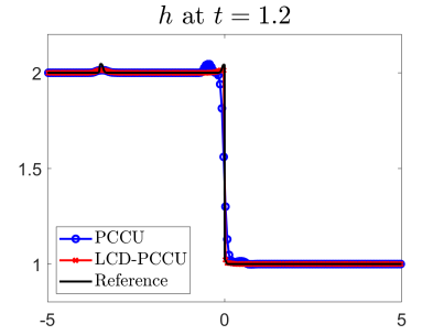
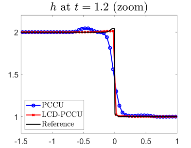
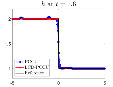
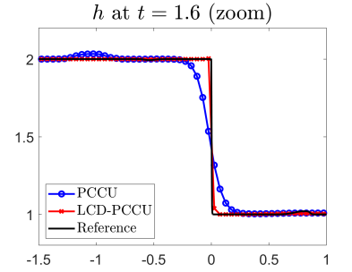
We then test the ability of the proposed schemes to capture small perturbations of this steady state. To this end, we first denote by given by (5.3), and then modify the initial condition of in the following manner:
We compute the solution until the final time on a uniform mesh with and plot the obtained fluid thickness at different times and 1.6 in Figure 5.9 together with the reference solution computed by the LCD-PCCU scheme on a much finer mesh with . One can clearly see that the LCD-PCCU scheme achieves sharper resolution than the PCCU scheme. Moreover, the LCD-PCCU solution is substantially less oscillatory than the PCCU one.
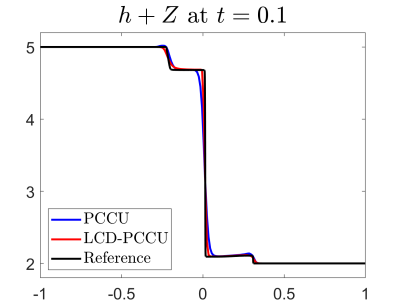
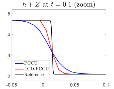
Example 7—Dam Break Over a Nonflat Bottom
In the second example taken from [16], we consider the dam break problem subject to the following initial data:
and the nonflat bottom topography
The initial conditions are prescribed in the computational domain subject to the free boundary conditions.
We compute the numerical solution by the PCCU and LCD-PCCU schemes until the final time on a uniform mesh with and plot the obtained water surface in Figure 5.10, where the reference solution is computed by the PCCU scheme on a much finer mesh with . One can clearly see that the LCD-PCCU scheme produces higher-resolution results than the PCCU one.
5.2.2 Two-Dimensional Examples
In this section, we consider three numerical examples for the 2-D TRSW equations.
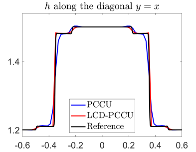
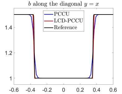
Example 8—Small Perturbations of a 2-D Steady State
In this example taken from [16], we take and consider the following initial conditions:
with the nonflat bottom topography consisting of two Gaussian shaped humps:
The initial data are prescribed in the computational domain subject to the free boundary conditions.
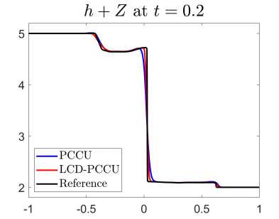
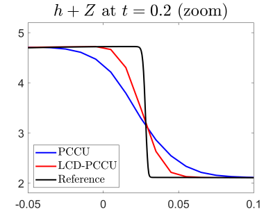
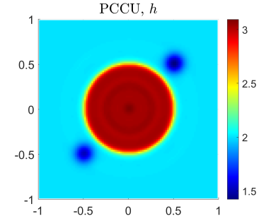
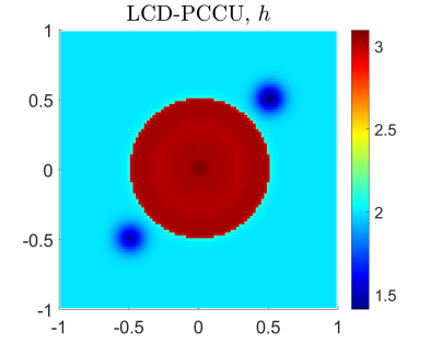
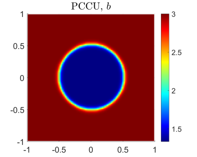
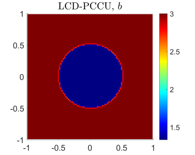
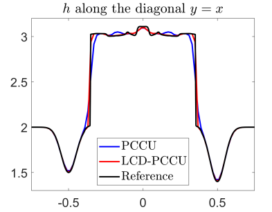
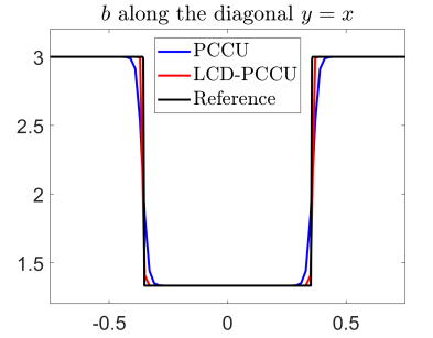
We compute the numerical solution by the PCCU and LCD-PCCU schemes until the final time on a uniform mesh with . The obtained results are presented in Figure 5.11, where one can clearly see that the LCD-PCCU scheme outperforms the PCCU one, since the - and -components computed by the PCCU scheme are smeared; see Figure 5.11. We also plot the 1-D slices of and along the diagonal ; see Figure 5.12, where the reference solution is computed by the PCCU scheme on a much finer mesh with . As one can see, the LCD-PCCU scheme achieves higher resolution than the PCCU one.
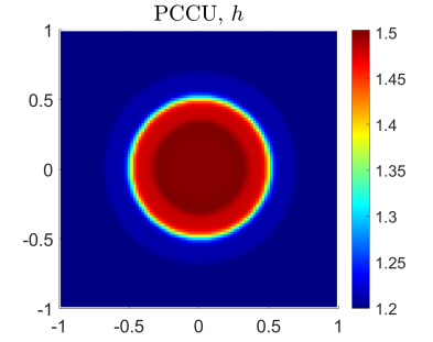
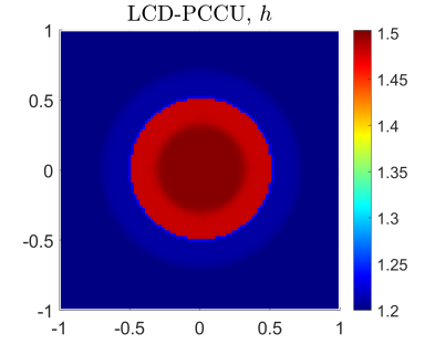
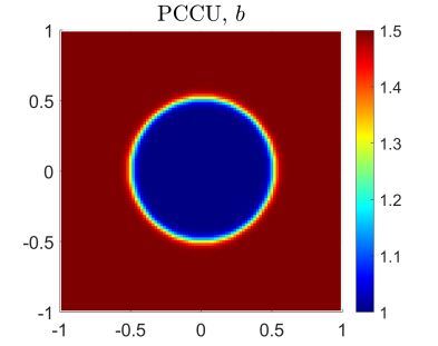
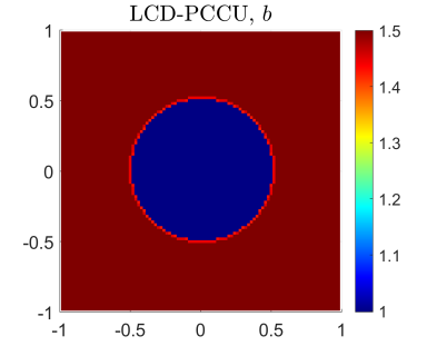
Example 9—Radial Dam Break Over the Flat Bottom
In this example taken from [16], we compare the PCCU and LCD-PCCU schemes on a circular dam-break problem with a flat bottom topography () and no Coriolis forces . The initial conditions,
are prescribed in the computational domain subject to the free boundary conditions.
We compute the numerical solution by the PCCU and LCD-PCCU schemes until the final time on a uniform mesh with . The computed results are presented in Figure 5.13, where one can clearly see that the LCD-PCCU scheme outperforms the PCCU scheme. We also plot the 1-D slices of and along the diagonal ; see Figure 5.14, where the reference solution is computed by the PCCU scheme on a much finer mesh with . As one can see, the LCD-PCCU scheme outperforms its PCCU counterpart.
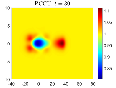
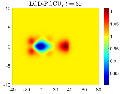
Example 10—Relaxation of Localized Anomalies on the Equatorial -Plane
In the last example taken from [27], we consider the relaxation of localized anomalies on the -plane, where the Coriolis parameter is , with the initial data
prescribed in the computational domain subject to the free boundary conditions.
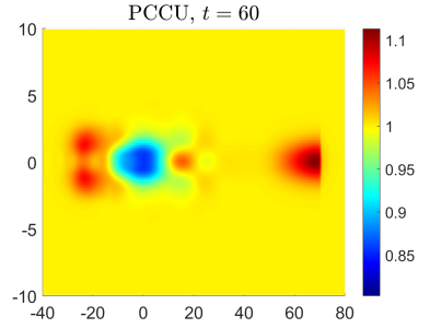
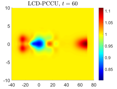
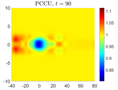
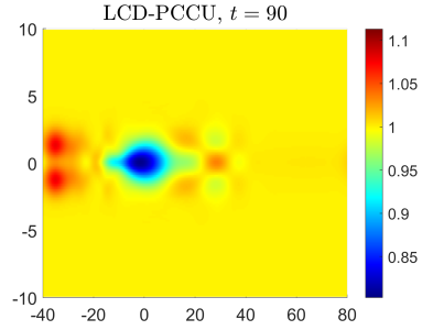
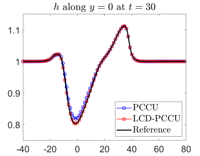
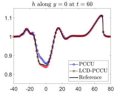
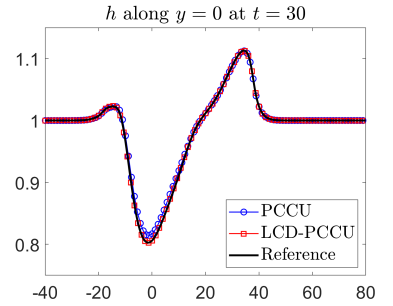
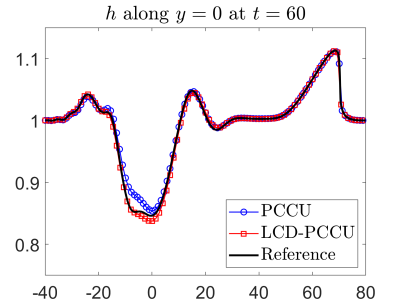
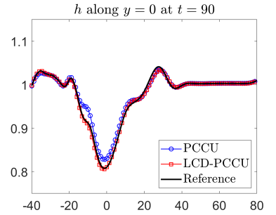
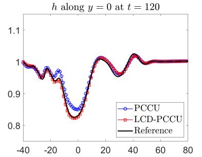
We compute the numerical solution by the PCCU and LCD-PCCU schemes until the final time on a uniform mesh with and plot the obtained numerical results in Figure 5.15, where one can see that our results are consistent with those reported in [27], and at the same time, the LCD-PCCU scheme outperforms the PCCU one. In order to better see the difference between the computed solutions, we also plot the 1-D slices of along in Figure 5.16, where the reference solution is computed by the PCCU scheme on a finer mesh with . One can see that the LCD-PCCU scheme achieves significantly better resolution than the PCCU one.
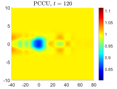
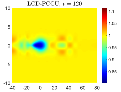
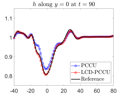
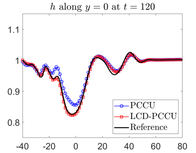
In this example, we also check the efficiency of the proposed LCD-PCCU scheme by performing a more thorough comparison between the studied schemes. To this end, we measure the CPU time consumed during the above calculations by the LCD-PCCU scheme and refine the mesh used by the PCCU scheme to the level that exactly the same CPU time is consumed to compute both of the numerical solutions: This way, we take into account additional computational cost of the LCD-PCCU scheme. The corresponding grids are for the LCD-PCCU scheme, and for the PCCU scheme. The obtained numerical results are plotted in Figure 5.17, where one can clearly see that the LCD-PCCU solution is still more accurate than the PCCU one.
Acknowledgments
The work of Michael Herty was funded by the Deutsche Forschungsgemeinschaft (DFG, German Research Foundation)–SPP 2183: Eigenschaftsgeregelte Umformprozesse with the Project(s) HE5386/19-2,19-3 Entwicklung eines flexiblen isothermen Reckschmiedeprozesses für die eigenschaftsgeregelte Herstellung von Turbinenschaufeln aus Hochtemperaturwerkstoffen (424334423) and by the Deutsche Forschungsgemeinschaft (DFG, German Research Foundation)–SPP 2410 Hyperbolic Balance Laws in Fluid Mechanics: Complexity, Scales, Randomness (CoScaRa) within the Project(s) HE5386/26-1 (Numerische Verfahren für gekoppelte Mehrskalenprobleme,525842915) and (Zufällige kompressible Euler Gleichungen: Numerik und ihre Analysis, 525853336) HE5386/27-1. The work of A. Kurganov was supported in part by NSFC grant 12171226 and by the fund of the Guangdong Provincial Key Laboratory of Computational Science and Material Design (No. 2019B030301001).
Appendix A LCD Matrices for the -Based Compressible Multifluid Equations
A.1 One-Dimensional Case
In order to compute the LCD matrices for the 1-D -based compressible multifluid system, we first compute the matrix :
| (A.1) |
where is the speed of sound, and then introduce , which is given by (A.1) with , , , and replaced with
respectively. Here,
Notice that all of the quantities have to have a subscript index, that is, , but we omit it for the sake of brevity for all of the quantities except for . We then compute the matrix composed of the right eigenvectors of and obtain
A.2 Two-Dimensional Case
We now compute the matrix and the corresponding matrices and for the 2-D -based compressible multifluid system.
We first compute :
|
|
(A.2) |
and then introduce the matrix , which is given by (A.2) with , , , , and replaced with
respectively. Here,
Notice that all of the quantities have to have a subscript index, that is, , but we omit it for the sake of brevity for all of the quantities except for . We then compute the matrix composed of the right eigenvectors of and obtain
Appendix B LCD Matrices for the TRSW Equations
B.1 One-dimensional Case
In order to compute the LCD matrices for the 1-D TRSW equations, we first compute the matrix :
| (B.1) |
and then introduce the matrices , which are given by (B.1) with , , , and replaced with
respectively. Here, , , and .
Notice that all of the quantities have to have a subscript index, that is, , but we omit it for the sake of brevity for all of the quantities except for . We then compute the matrix composed of the right eigenvectors of and obtain
B.2 Two-Dimensional Case
We now compute the matrix and the corresponding matrices and for the 2-D TRSW equations.
We first compute :
| (B.2) |
and then introduce the matrices , which are given by (B.2) with , , , and replaced with
respectively. Here , , and .
Notice that all of the quantities have to have a subscript index, that is, , but we omit it for the sake of brevity for all of the quantities except for . We then compute the matrix composed of the right eigenvectors of and obtain
References
- [1] S. Busto, M. Dumbser, S. Gavrilyuk, and K. Ivanova, On thermodynamically compatible finite volume methods and path-conservative ADER discontinuous Galerkin schemes for turbulent shallow water flows, J. Sci. Comput., 88 (2021). Paper No. 28, 45 pp.
- [2] Y. Cao, A. Kurganov, and Y. Liu, Flux globalization based well-balanced path-conservative central-upwind scheme for the thermal rotating shallow water equations, Commun. Comput. Phys., 34 (2023), pp. 993–1042.
- [3] Y. Cao, A. Kurganov, Y. Liu, and R. Xin, Flux globalization based well-balanced path-conservative central-upwind schemes for shallow water models, J. Sci. Comput., 92 (2022). Paper No. 69, 31 pp.
- [4] Y. Cao, A. Kurganov, Y. Liu, and V. Zeitlin, Flux globalization based well-balanced path-conservative central-upwind scheme for two-layer thermal rotating shallow water equations, J. Comput. Phys., 474 (2023). Paper No. 111790, 29 pp.
- [5] V. Caselles, R. Donat, and G. Haro, Flux-gradient and source-term balancing for certain high resolution shock-capturing schemes, Comput. & Fluids, 38 (2009), pp. 16–36.
- [6] M. J. Castro, T. Morales de Luna, and C. Parés, Well-balanced schemes and path-conservative numerical methods, in Handbook of numerical methods for hyperbolic problems, vol. 18 of Handb. Numer. Anal., Elsevier/North-Holland, Amsterdam, 2017, pp. 131–175.
- [7] M. J. Castro and C. Parés, Well-balanced high-order finite volume methods for systems of balance laws, J. Sci. Comput., 82 (2020). Paper No. 48, 48 pp.
- [8] M. J. Castro Díaz, A. Kurganov, and T. Morales de Luna, Path-conservative central-upwind schemes for nonconservative hyperbolic systems, ESAIM Math. Model. Numer. Anal., 53 (2019), pp. 959–985.
- [9] C. Chalons, Path-conservative in-cell discontinuous reconstruction schemes for non conservative hyperbolic systems, Commun. Math. Sci., 18 (2020), pp. 1–30.
- [10] Y. Chen, A. Kurganov, and M. Na, A Flux Globalization Based Well-Balanced Path-Conservative Central-Upwind Scheme for the Shallow Water Flows in Channels, ESAIM Math. Model. Numer. Anal., 57 (2023), pp. 1087–1110.
- [11] J. Cheng, F. Zhang, and T. G. Liu, A discontinuous Galerkin method for the simulation of compressible gas-gas and gas-water two-medium flows, J. Comput. Phys., 403 (2020). Paper No. 109059, 29 pp.
- [12] A. Chertock, S. Chu, M. Herty, A. Kurganov, and M. Lukáčová-Medviďová, Local characteristic decomposition based central-upwind scheme, J. Comput. Phys., 473 (2023). Paper No. 111718, 24 pp.
- [13] A. Chertock, S. Chu, and A. Kurganov, Hybrid multifluid algorithms based on the path-conservative central-upwind scheme, J. Sci. Comput., 89 (2021). Paper No. 48, 24 pp.
- [14] A. Chertock, M. Herty, and Ş. N. Özcan, Well-balanced central-upwind schemes for systems of balance laws, in Theory, Numerics and Applications of Hyperbolic Problems. I, C. Klingenberg and M. Westdickenberg, eds., vol. 236 of Springer Proc. Math. Stat., Springer, Cham, 2018, pp. 345–361.
- [15] A. Chertock, S. Karni, and A. Kurganov, Interface tracking method for compressible multifluids, M2AN Math. Model. Numer. Anal., 42 (2008), pp. 991–1019.
- [16] A. Chertock, A. Kurganov, and Y. Liu, Central-upwind schemes for the system of shallow water equations with horizontal temperature gradients, Numer. Math., 127 (2014), pp. 595–639.
- [17] S. Chu, A. Kurganov, and R. Xin, Low-dissipation central-upwind schemes for compressible multifluids, Submitted. Preprint available at https://sites.google.com/view/alexander-kurganov/publications.
- [18] S. Chu, A. Kurganov, and R. Xin, A well-balanced fifth-order A-WENO scheme based on flux globalization, Submitted. Preprint available at https://sites.google.com/view/alexander-kurganov/publications.
- [19] G. Dal Maso, P. G. Lefloch, and F. Murat, Definition and weak stability of nonconservative products, J. Math. Pures Appl., 74 (1995), pp. 483–548.
- [20] D. Donat and A. Martinez-Gavara, Hybrid second order schemes for scalar balance laws, J. Sci. Comput., 48 (2011), pp. 52–69.
- [21] L. Gascón and J. M. Corderán, Construction of second-order TVD schemes for nonhomogeneous hyperbolic conservation laws, J. Comput. Phys., 172 (2001), pp. 261–297.
- [22] S. Gottlieb, D. Ketcheson, and C.-W. Shu, Strong stability preserving Runge-Kutta and multistep time discretizations, World Scientific Publishing Co. Pte. Ltd., Hackensack, NJ, 2011.
- [23] S. Gottlieb, C.-W. Shu, and E. Tadmor, Strong stability-preserving high-order time discretization methods, SIAM Rev., 43 (2001), pp. 89–112.
- [24] J.-F. Haas and B. Sturtevant, Interaction of weak shock waves with cylindrical and spherical gas inhomogeneities, J. Fluid Mech., 181 (1987), pp. 41–76.
- [25] A. Kurganov and C.-T. Lin, On the reduction of numerical dissipation in central-upwind schemes, Commun. Comput. Phys., 2 (2007), pp. 141–163.
- [26] A. Kurganov, Y. Liu, and R. Xin, Well-balanced path-conservative central-upwind schemes based on flux globalization, J. Comput. Phys., 474 (2023). Paper No. 111773, 32 pp.
- [27] A. Kurganov, Y. Liu, and V. Zeitlin, Thermal versus isothermal rotating shallow water equations: comparison of dynamical processes by simulations with a novel well-balanced central-upwind scheme, Geophys. Astrophys. Fluid Dyn., 115 (2021), pp. 125–154.
- [28] A. Kurganov, S. Noelle, and G. Petrova, Semidiscrete central-upwind schemes for hyperbolic conservation laws and Hamilton-Jacobi equations, SIAM J. Sci. Comput., 23 (2001), pp. 707–740.
- [29] A. Kurganov and E. Tadmor, New high-resolution semi-discrete central schemes for Hamilton-Jacobi equations, J. Comput. Phys., 160 (2000), pp. 720–742.
- [30] Philippe G. LeFloch, Hyperbolic systems of conservation laws, Lectures in Mathematics ETH Zürich, Birkhäuser Verlag, Basel, 2002. The theory of classical and nonclassical shock waves.
- [31] P. G. Lefloch, Graph solutions of nonlinear hyperbolic systems, J. Hyperbolic Differ. Equ., 1 (2004), pp. 643–689.
- [32] K.-A. Lie and S. Noelle, On the artificial compression method for second-order nonoscillatory central difference schemes for systems of conservation laws, SIAM J. Sci. Comput., 24 (2003), pp. 1157–1174.
- [33] A. Martinez-Gavara and R. Donat, A hybrid second order scheme for shallow water flows, J. Sci. Comput., 48 (2011), pp. 241–257.
- [34] H. Nessyahu and E. Tadmor, Nonoscillatory central differencing for hyperbolic conservation laws, J. Comput. Phys., 87 (1990), pp. 408–463.
- [35] C. Parés, Path-conservative numerical methods for nonconservative hyperbolic systems, vol. 24 of Quad. Mat., Dept. Math., Seconda Univ. Napoli, Caserta, 2009.
- [36] E. Pimentel-García, M. J. Castro, C. Chalons, T. Morales de Luna, and C. Parés, In-cell discontinuous reconstruction path-conservative methods for non conservative hyperbolic systems—second-order extension, J. Comput. Phys., 459 (2022). Paper No. 111152, 35 pp.
- [37] J. J. Quirk and S. Karni, On the dynamics of a shock-bubble interaction., J. Fluid Mech., 318 (1996), pp. 129–163.
- [38] K. A. Schneider, J. M. Gallardo, D. S. Balsara, B. Nkonga, and C. Parés, Multidimensional approximate Riemann solvers for hyperbolic nonconservative systems. Applications to shallow water systems, J. Comput. Phys., 444 (2021). Paper No. 110547, 49 pp.
- [39] K.-M. Shyue, An efficient shock-capturing algorithm for compressible multicomponent problems, J. Comput. Phys., 142 (1998), pp. 208–242.
- [40] P. K. Sweby, High resolution schemes using flux limiters for hyperbolic conservation laws, SIAM J. Numer. Anal., 21 (1984), pp. 995–1011.
- [41] L. Xu and T. G. Liu, Explicit interface treatments for compressible gas-liquid simulations, Comput. & Fluids, 153 (2017), pp. 34–48.