SlotGAT: Slot-based Message Passing for Heterogeneous Graph Neural Network

Abstract

Heterogeneous graphs are ubiquitous to model complex data. There are urgent needs on powerful heterogeneous graph neural networks to effectively support important applications. We identify a potential semantic mixing issue in existing message passing processes, where the representations of the neighbors of a node $v$ are forced to be transformed to the feature space of $v$ for aggregation, though the neighbors are in different types. That is, the semantics in different node types are entangled together into node $v$’s representation. To address the issue, we propose SlotGAT with separate message passing processes in slots, one for each node type, to maintain the representations in their own node-type feature spaces. Moreover, in a slot-based message passing layer, we design an attention mechanism for effective slot-wise message aggregation. Further, we develop a slot attention technique after the last layer of SlotGAT, to learn the importance of different slots in downstream tasks. Our analysis indicates that the slots in SlotGAT can preserve different semantics in various feature spaces. The superiority of SlotGAT is evaluated against 13 baselines on 6 datasets for node classification and link prediction. Our code is at https://github.com/scottjiao/SlotGAT_ICML23/.

1 Introduction

Heterogeneous graphs with node and edge types (Hu et al., 2020a; Dong et al., 2017; Yang et al., 2020a), are ubiquitous in many real applications, e.g., protein prediction (Fout et al., 2017), recommendation (Fan et al., 2019; Yang et al., 2020b), social analysis (Qiu et al., 2018; Li & Goldwasser, 2019), and traffic prediction (Guo et al., 2019). Figure 1(a) displays a heterogeneous academic graph with 5 nodes in 3 types, i.e., author, paper, venue. Usually edge type is related to the node types of the two ends of an edge. For instance, the edge between $v_{1}$ (author) and $v_{2}$ (paper) is an authorship edge; $v_{2}$ and $v_{5}$ (paper) have a citation edge.

Heterogeneous graphs have attracted great research attentions. Conventional graph neural networks (GNNs) (Hamilton et al., 2017; Klicpera et al., 2019; Kipf & Welling, 2017; Velickovic et al., 2018; Monti et al., 2017; Liu et al., 2020) can be applied by regarding heterogeneous graphs as homogeneous ones. GNNs are good enough, but still ignore the heterogeneous semantics (Lv et al., 2021). Hence, several heterogeneous graph neural networks (HGNNs) are developed (Wang et al., 2019d; Yun et al., 2019; Zhu et al., 2019; Zhang et al., 2019; Fu et al., 2020; Hu et al., 2020b; Hong et al., 2020; Schlichtkrull et al., 2018; Cen et al., 2019; Wang et al., 2019b, a, c; Lv et al., 2021; Zhao et al., 2022). Some HGNNs rely on meta-paths, either predefined manually (Wang et al., 2019d; Fu et al., 2020) or learned automatically (Yun et al., 2019), which incur extra costs. Then there are studies of relation oriented HGNNs (Zhu et al., 2019; Schlichtkrull et al., 2018), HGNNs with random walks and RNNs (Zhang et al., 2019), empowering GNNs for HGNNs (Lv et al., 2021), etc. Zhao et al. (2022) define a unified design space for HGNNs.

It is known that different node types have different semantics, and naturally should have different impacts (Wang et al., 2019d; Lv et al., 2021; Hu et al., 2020b). However, when aggregating the messages from different types of nodes, the semantics are mixed in existing work, which may hamper the effectiveness (Wang et al., 2019d; Yun et al., 2019; Zhu et al., 2019; Fu et al., 2020). Specifically, in existing message passing layers, when a node $v$ aggregates messages from its neighbors $u$ that may be in different node type, they force the representation of $u$ in another type-specific feature space to be transformed to the feature space of $v$’s type, and then aggregate the transformed message to $v$. We argue that this forced transformation mixes different feature spaces, making representations entangled with each other. This semantic mixing issue is illustrated in Figure 1(c). Given the heterogeneous graph in the figure, every node is with a single initial representation as input. Then in Layer 1, when node $v_{2}$ (paper type id 1) aggregates the message from its neighbor $v_{1}$ (author type id 0) in a different node type, it first applies a transformation $\tau(0,1)$ to convert the representation of $v_{1}$ from author’s feature space to paper’s feature space, and then aggregates it to paper $v_{2}$’s representation. Similar forced transformation also exists when aggregating $v_{3}$ (venue) to $v_{2}$ (paper) in Layer 1. Instead of converting all $v$’s neighboring representations to $v$’s feature space, if we separate and preserve the impacts of different node-type features to $v$, we could learn more effective representations.

Hence, we propose SlotGAT, which has separate message slots of different node types (i.e., feature spaces), with dedicated attention mechanisms to measure the importance of slots. SlotGAT conducts slot-based message passing processes to alleviate the semantic mixing issue. We explain the idea of slot-based message passing in Figure 1(b). For a node $v$, we maintain a slot for every node type in the heterogeneous graph, e.g., every node with 3 slots in Figure 1(b) for author, paper, venue types, respectively. When initializing the input slot representations of $v_{2}$ (paper), the slot for paper type (slot 1) is initialized by $v_{2}$’s features, while other slots (slots 0, 2) of $v_{2}$ for author and venue are initialized as empty. In Layer 1, when aggregating neighbors to $v_{2}$, the slot 0 message from $v_{1}$ is aggregated to the corresponding slot 0 of $v_{2}$, without mixing with the representations in other slots (i.e., other node types). The slot 2 message from $v_{3}$ (venue) is aggregated to the respective slot 2 of $v_{2}$. Obviously, though $v_{2}$ is in paper type, it can maintain slot representations of other node types, compared with existing methods in Figure 1(c) where $v_{2}$ mixes the representations of $v_{1}$, $v_{2}$, $v_{3}$, $v_{5}$ in different node types. In the layers of SlotGAT, we also design an attention-based aggregation mechanism that considers all slot representations of a node and its neighbors as well as edge type representations for aggregation. In downstream tasks, to effectively integrate the slot representations of a node, after the last layer of SlotGAT, we develop a slot attention technique to learn the importance of different slots. Our analysis indicates that SlotGAT can preserve different semantics into slots.

Compared with numerous existing methods, SlotGAT achieves superior performance on all datasets under various evaluation metrics. We also conduct model analysis, including statistical significance test, visualization, and ablation analysis, to analyze the effectiveness of SlotGAT.

We summarize our contributions as follows:

• We propose a novel slot-based heterogeneous graph neural network model SlotGAT for heterogeneous graphs.

• We develop a new slot-based message passing mechanism, so that semantics of different node-type feature spaces do not entangle with each other.

• We further design attention mechanisms to effectively process the representations in slots.

• Extensive experiments demonstrate the superiority of SlotGAT on real-world heterogeneous graphs.

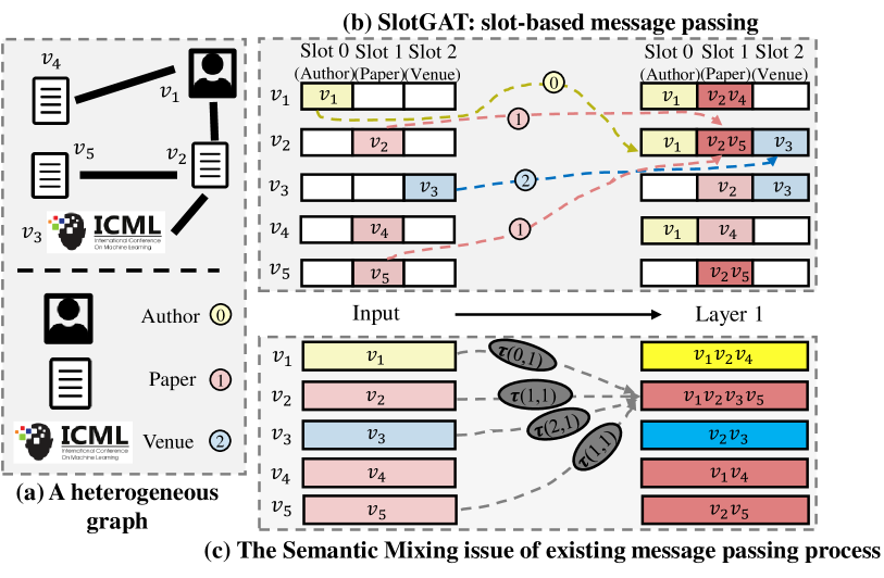
Figure 1: (a) A heterogeneous graph. (b) The slot-based message passing in the proposed SlotGAT: every node has 3 slots, corresponding to 3 node-type feature spaces. For example, in the input layer, $v_{2}$’s slot 1 is initialized by its features since $v_{2}$ is in type 1, while slots 0 and 2 of $v_{2}$ are empty. The message passing in SlotGAT is slot specific (colored dashed arrows), e.g., neighboring slot messages passed to the slots of the same node type on node $v_{2}$ in Layer 1. (c) The semantic mixing issue: every node maintains a single representation; in Layer 1, $v_{2}$ aggregates message from $v_{1}$ by firstly applying transformation $\tau(0,1)$ to convert $v_{1}$’s representation in type 0 to the feature space of $v_{2}$ in type 1, which mixes the two feature spaces.

2 Preliminary

A heterogeneous graph is $\mathcal{G}=\left(\mathcal{V},{\mathcal{E}},\phi,\psi\right)$, where $\mathcal{V}$ is the set of nodes, ${\mathcal{E}}$ is the set of edges, $\phi$ is a node type mapping function, and $\psi$ is an edge type mapping function. Every node $v$ has node type $\phi(v)$, and every edge $e=(v,u)$ has edge type $\psi(e)$, also denoted as $\psi(v,u)$. Let $\Phi$ and $\Psi$ be the set of all node types and the set of all edge types respectively in graph $\mathcal{G}$. Assume that node types in $\Phi$ are represented by consecutive integers starting from $0$, and denote $t$ as the $t$-th node type. Let $n$ be the number of nodes, i.e., $n=|\mathcal{V}|$, and $m$ be the number of edges, i.e., $m=|{\mathcal{E}}|$. For a heterogeneous graph $|\Psi|+|\Phi|>2$.

A node $v$ has a feature vector $\mathbf{x}_{v}$. For node type $t\in\Phi$, all type-$t$ nodes $v\in\{v\in{\mathcal{V}}|\phi(v)=t\}$ have the same feature dimension $d_{0}^{t}=d_{0}^{\phi(v)}$, i.e., $\mathbf{x}_{v}\in^{d_{0}^{\phi(v)}}$. Nodes of different types can have different feature dimensions (Lv et al., 2021).

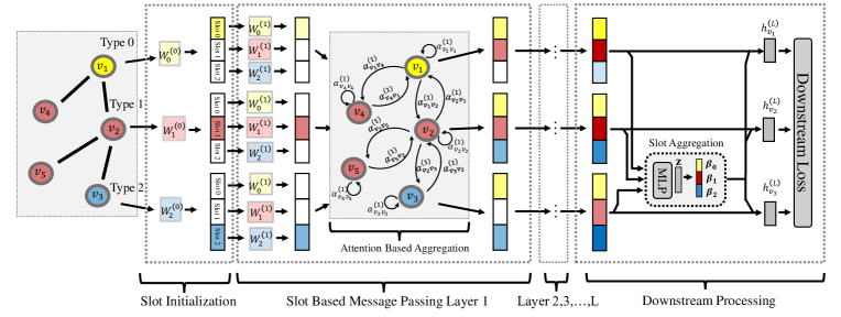
Figure 2: The SlotGAT architecture. (i) SlotGAT initializes every node with multiple slots corresponding to all node types (3 types in the example), and the slot for the node’s type is initialized by its transformed features, while the other slots are empty. (ii) In a slot-based message passing layer, slot representations are transformed and propagated separately, with an attention based aggregation technique. (iii) After the last $L$-th layer, SlotGAT includes a slot attention technique to integrate slots for downstream tasks.

3 Related Work

Homogeneous GNNs handle graphs without node/edge types (Kipf & Welling, 2017; Liu et al., 2020; Bruna et al., 2014; Defferrard et al., 2016; Velickovic et al., 2018; Monti et al., 2017; Chen et al., 2020b; Klicpera et al., 2019). GCN (Kipf & Welling, 2017) simplifies spectral networks on graphs (Bruna et al., 2014) into its GNN form. GAT (Velickovic et al., 2018) introduces self-attention to GNNs. Then, there is a plethora of HGNNs to handle heterogeneous graphs. Meta-paths are used in (Wang et al., 2019d; Fu et al., 2020; Yun et al., 2019). HAN (Wang et al., 2019d) consists of a hierarchical attention mechanism to capture node-level importance between nodes and semantic-level importance of meta-paths. MAGNN (Fu et al., 2020) is an enhanced method with several meta-path encoders to encode all the information along meta-paths. Both MAGNN and HAN require meta-paths generated manually. Graph transformer network (GTN) (Yun et al., 2019) can automatically learn meta-paths with graph transformation layers. For heterogeneous graphs with many edge types, meta-path based methods are not easily applicable, due to the high cost on obtaining meta-paths. There are methods treating heterogeneous graphs as relation graphs to develop graph neural network methods. RSHN is a relation structure-aware HGNN (Zhu et al., 2019), which builds coarsened line graph to get edge features and adopts a Message Passing Neural Network (MPNN) (Gilmer et al., 2017) to propagate node and edge features. RGCN (Schlichtkrull et al., 2018) splits a heterogeneous graph to multiple subgraphs by building an independent adjacency matrix for each edge type. Furthermore, HGT (Hu et al., 2020b) is a graph transformer model to handle large heterogeneous graphs with heterogeneous subgraph sampling techniques. HetGNN (Zhang et al., 2019) uses random walks to sample fixed-size neighbors for nodes in different node type, and then applies RNNs for representation learning. As shown in experiments, HetGNN is inferior to our method. HetSANN (Hong et al., 2020) contains type-specific graph attention layers to aggregate local information. In experiments, SlotGAT is better than HetSANN. Recently, Lv et al., (Lv et al., 2021) develop simpleHGN with several techniques on homogeneous GNNs to handle heterogeneous graphs. Space4HGNN (Zhao et al., 2022) defines a unified design space for HGNNs, to exhaustively evaluate the combinations of many techniques. Wang et al. (2020) propose a disentangled mechanism in which an aspect of a target node aggregates semantics from all neighbors for recommendation, regardless of node types. Contrarily, we learn separate semantics in different node type feature spaces, which is different.

4 The SlotGAT Method

Figure 2 shows the architecture of SlotGAT, consisting of node-type slot initialization, slot-based message passing layers with attention based aggregation, and a slot attention module.

Given a heterogeneous graph $\mathcal{G}$, SlotGAT creates $|\Phi|$ slots for every node (3 slots per node in Figure 2). The $t$-th slot of a node $v$ represents the semantic representation of $v$ with respect to node type $t$. For initialization, as in Figure 2, if slot $t$ of $v$ (e.g., $v_{3}$) corresponds to the node type of $v$, $\phi(v)$ (e.g., $t=2$), then slot $t$ is initialized by node $v$’s features $\mathbf{x}_{v}$ via a linear transformation. All other slots of $v$ are initialized as zero (e.g., slots 0, 1 of $v_{3}$ in Figure 2).

Then within a slot-based message passing layer of SlotGAT, given a node $v$, its neighbors transform and pass slot-wise messages to it. Compared with existing methods that only pass one message from a neighbor $u$ to $v$, SlotGAT passes $|\Phi|$ slot messages separately to $v$, and these messages do not mix with each other in intermediate layers. As illustrated in Figure 2, in Layer $l=1$, for any neighbor $u$ of $v$, we apply transformation by $\mathbf{W}_{t}^{(l)}$ independently on each slot $t$ of $u$, and then pass the transformed slot messages to $v$ for slot-wise aggregation with an attention mechanism that leverages slot representations and edge types to compute attention scores, elaborated in Section 4.2. Remark that the slot $t$ of $v$ preserves the type-$t$ specific semantics delivered from the graph to $v$, regardless whether $v$ is in type $t$ or not. With this novel slot-based message passing in a layer, SlotGAT are able to maintain distinguishable representations of a node in a finer granularity.

After $L$ layers of slot-based message passing in SlotGAT, every node $v$ has $|\Phi|$ slot representations as shown in Figure 2. For downstream tasks, we develop a slot attention technique in Section 4.3 to learn slot importance scores to get final representations, which are then fed into downstream tasks. Algorithm 1 shows the pseudo code of SlotGAT.

4.1 Node Type Slot Initialization

We create $|\Phi|$ type-specific slots for every node. Then given a node $v$ with type $\phi(v)$, its slot $t$ $\mathbf{h}_{v}^{(0),t}$ is initialized by Eq. 1. Specifically, if slot $t$ is not type $\phi(v)$, then $\mathbf{h}_{v}^{(0),t}$ is set to zero initially; otherwise, $\mathbf{h}_{v}^{(0),t}$ is initialized by the feature vector of $v$ with a $t$ type-specific linear transformation $\mathbf{W}_{t}^{(0)}$. Since the feature vectors of different types of nodes can be in different dimensions, $\mathbf{W}_{t}^{(0)}$ is a pre-processor to map heterogeneous node features to the same dimension $d_{1}$.

$$\small\mathbf{h}_{v}^{(0),t}= \begin{cases}\mathbf{W}_{t}^{(0)}\mathbf{x}_{v}\in^{d_{1}}&\text{ if }t=\phi(v),\\ \mathbf{0}\in^{d_{1}}&\text{ if }t\neq\phi(v),\end{cases}$$ (1)

where $\mathbf{W}_{t}^{(0)}\in^{d_{1}\times d_{0}^{\phi(v)}}$ is a $t$-type transformation matrix.

4.2 Slot-based Message Passing Layer

In this section, we present the slot-based message passing layer of SlotGAT with slot-specific transformations and a new attention mechanism.

In the $l$-th layer of SlotGAT, all $t$-type slots of all nodes in $\mathcal{G}$ maintain type-specific (or slot-specific) transformations $\mathbf{W}_{t}^{(l)}$. Given a node $v$ with slot $t$ representation $\mathbf{h}_{v}^{(l-1),t}$ from the $(l-1)$-th layer, in current $l$-th layer, the representation is transformed to $\hat{\mathbf{h}}_{v}^{(l),t}$ by $\mathbf{W}_{t}^{(l)}$ in Eq. 2. Note that the transformation is within the feature space of node type $t$, and does not affect the feature spaces of other types.

$$\small\hat{\mathbf{h}}_{v}^{(l),t}=\mathbf{W}_{t}^{(l)}\mathbf{h}_{v}^{(l-1),t},$$ (2)

where $\mathbf{W}_{t}^{(l)}\in^{d_{l}\times d_{l-1}}$ is a slot-specific transformation.

For instance, in Figure 2, in the first layer, the transformation matrix $\mathbf{W}_{1}^{(1)}$ for slot $1$ (in red) is applied to the slots 1 of all nodes. Even if the node is not in type $t=1$, its slot 1 will be transformed by $\mathbf{W}_{1}^{(1)}$. Observe that, if a slot is empty, its message will still be zero vector after transformation.

In the $l$-th layer of SlotGAT ($0<l\leq L$), for every slot $t$ of every node $v\in\mathcal{V}$ ($t\in\Phi$), we perform the above type-specified linear transformation to get slot messages $\hat{\mathbf{h}}_{v}^{(l),t}$, which will be aggregated in the $l$-th layer via a generic slot-based message aggregation function $aggr$. In particular, given a node $v$, its slot $t$ receives messages $\hat{\mathbf{h}}_{u}^{(l),t}$ from its neighbors $u\in N(v)$, which are then aggregated to update its slot $t$ to be $\mathbf{h}_{v}^{(l),t}$,

$$\small\mathbf{h}_{v}^{(l),t}=aggr\left(\{\hat{\mathbf{h}}_{u}^{(l),t}\}_{u\in N(v)}\right),\forall t\in\Phi,$$ (3)

where $\mathbf{h}_{v}^{(l),t}\in^{d_{l}}$, $\mathbf{h}_{v}^{(l),t}\in^{d_{l}}$.

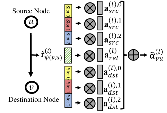
Figure 3: Attention mechanism in a message passing layer.

Observe that in the propagation and aggregation process above, SlotGAT uses the whole graph topology to propagate slot messages. Moreover, there can be multiple options for the $aggr$ function, e.g., mean and max (Hamilton et al., 2017). Instead of using these vanilla aggregation functions, we develop an attention mechanism to learn the aggregation weights $\alpha^{(l)}_{vu}$ in Eq. 4, where the aggregation result is then passed via non-linear ReLu activation $\sigma$.

$$\small\mathbf{h}_{v}^{(l),t}=\sigma\left(\sum_{u\in N(v)}\alpha^{(l)}_{vu}\hat{\mathbf{h}}_{u}^{(l),t}\right),\forall t\in\Phi.$$ (4)

Now we elaborate how to get aggregation weight $\alpha^{(l)}_{vu}$. Intuitively, node $u$ passes all its slot messages to $v$ for all slots $t\in\Phi$. Thus, weight $\alpha^{(l)}_{vu}$ should be computed by considering all the slot messages from $u$ to $v$, as well as edge types, instead of only using a specific slot $t$. In other words, all slot messages from node $u$ to $v$ share the same aggregation weight. Specifically,we develop a self-attention technique with slot message encoders and edge-type encoders to compute $\alpha^{(l)}_{vu}\in$, as illustrated in Figure 3. In the $l$-th layer, all nodes serving as the source of messages (e.g., $u$ in Figure 3) share a slot-specific attention vector $\mathbf{a}^{(l),t}_{src}\in^{d_{l}}$ for every $t\in\Phi$. Similarly, all nodes that serve as the destination to receive messages (e.g., $v$ in Figure 3) share a slot-specific attention vector $\mathbf{a}^{(l),t}_{dst}\in^{d_{l}}$ for every $t\in\Phi$. Further, let $\mathbf{a}^{(l)}_{rel}\in^{d_{e}}$ be an attention vector for edge types. Then the overall attention vector $\mathbf{a}^{(l)}$ is obtained by

$$\small\mathbf{a}^{(l)}=\left(\bigparallel_{t\in\Phi}\mathbf{a}^{(l),t}_{src}\right)\Big{|}\left(\bigparallel_{t\in\Phi}\mathbf{a}^{(l),t}_{dst}\right)\Big{|}\mathbf{a}^{(l)}_{rel}.$$ (5)

To get the edge type embedding of $l$-th layer, $\hat{\mathbf{r}}^{(l)}_{\psi(v,u)}$, we use a similar idea in (Lv et al., 2021). Let $\mathbf{r}_{\psi(v,u)}\in^{d_{e}}$ be a learnable representation of edge type $\psi(v,u)$, and it is randomly initialized and shared across all layers for all edges with type $\psi(v,u)$. It is transformed to get the $l$-th layer representation ${\textstyle\hat{\mathbf{r}}^{(l)}_{\psi(v,u)}=\mathbf{W}_{rel}^{(l)}\mathbf{r}_{\psi(v,u)}}$, where ${\textstyle\mathbf{W}_{rel}^{(l)}\in^{d_{e}\times d_{e}}}$ is a learnable matrix. Then we compute the attention score $\alpha_{vu}^{(l)}$ by Eq. 6 and 7. In Eq. 6, we first get an intermediate $\hat{\alpha}_{vu}^{(l)}$ by inner product between the corresponding attention vectors and representations, including source node’s slot representations ${\textstyle\hat{\mathbf{h}}_{u}^{(l),t}}$, destination node’s slot representations ${\textstyle\hat{\mathbf{h}}_{v}^{(l),t}}$, and edge type representations ${\textstyle\hat{\mathbf{r}}^{(l)}_{\psi(v,u)}}$. Then we use softmax normalization and LeakyReLU to get ${\textstyle\alpha^{(l)}_{vu}}$ in Eq. 7.

$$\small\hat{\alpha}_{vu}^{(l)}=\sum_{t\in\Phi}\langle\mathbf{a}^{(l),t}_{dst},\hat{\mathbf{h}}_{v}^{(l),t}\rangle+\sum_{t\in\Phi}\langle\mathbf{a}^{(l),t}_{src},\hat{\mathbf{h}}_{u}^{(l),t}\rangle+\langle\mathbf{a}^{(l)}_{rel},\hat{\mathbf{r}}^{(l)}_{\psi(v,u)}\rangle$$ (6)

$$\small\alpha^{(l)}_{vu}=\frac{\exp\left(\text{LeakyReLU}\left(\hat{\alpha}_{vu}^{(l)}\right)\right)}{\textstyle\sum_{u\in N(v)}\exp\left(\text{LeakyReLU}\left(\hat{\alpha}_{vu}^{(l)}\right)\right)}$$ (7)

After $L$ slot-based message passing layers, SlotGAT outputs the representation $\mathbf{h}^{(L),t}_{v}$ of every slot $t$ in every node $v\in\mathcal{V}$.

To provide stability to the training process, SlotGAT employs multi-head attention mechanism with $K$ heads (Wang et al., 2019d; Velickovic et al., 2018; Hu et al., 2020b),

$$\hat{\mathbf{h}}_{v,(k)}^{(l),t}= \mathbf{W}_{t,(k)}^{(l)}\mathbf{h}_{v}^{(l-1),t}\in^{d_{l}},$$ (8)

$$\mathbf{h}_{v}^{(l),t}= \textstyle\bigparallel_{k=1,2,...,K}\sigma\left(\textstyle\sum_{u\in N(v)}\alpha^{(l)}_{vu,(k)}\hat{\mathbf{h}}_{u,(k)}^{(l),t}\right),$$

where subscript $(k)$ represents the corresponding variables for the $k$-th head.

4.3 Slot Attention

After $L$ layers, SlotGAT returns slot representations $\mathbf{h}^{(L),t}_{v}$ for $|\Phi|$ slots of nodes $v\in\mathcal{V}$. To handle the downstream tasks with objectives to be elaborated in Section 4.4, we explain how to leverage all slot representations of node $v$ to get its final representation $\mathbf{h}_{v}$ by a slot attention technique.

Given the slot representations of node $v$, $\mathbf{h}^{(L),t}_{v},\forall t\in\Phi$, a simple way is to average them by Eq. 9, which however, does not differentiate slot importance.

$$\mathbf{h}_{v}=\frac{1}{|\Phi|}\textstyle\sum_{t\in\Phi}\mathbf{h}_{v}^{(L),t}.$$ (9)

Another way is to stack a fully connected layer,

$$\mathbf{h}_{v}=\mathbf{W}_{fc}\mathbf{h}_{v}^{(L),t},$$ (10)

where $\mathbf{W}_{fc}\in^{d_{task}\times(|\Phi|d_{L})}$ is a learnable matrix.

But the way above is not explainable to demonstrate the importance of different slots in different tasks. Therefore, we develop a slot attention technique (illustrated in Figure 4), which achieves better performance than the two ways above as validated in experiments.

Specifically, in slot attention, we first apply a one-layer MLP to transform every slot representation ${\textstyle\mathbf{h}_{v}^{(L),t}}$ of every node $v$ of the $L$-th layer to vector $\mathbf{s}_{v,t}$,

$$\mathbf{s}_{v,t}=\tanh\left(\mathbf{W}_{b}\mathbf{h}_{v}^{(L),t}+\mathbf{b}_{b}\right),$$ (11)

where ${\small\textstyle\mathbf{W}_{b}\in^{d_{s}\times d_{L}}}$, ${\small\textstyle\mathbf{b}_{b}\in^{d_{s}}}$ are weights and bias.

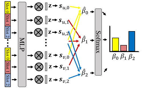
Figure 4: Slot attention

$\mathbf{s}_{v,t}$ represents the slot semantics decoded from slot $t$ of node $v$ in last $L$-th layer. Then, for each slot $t$, we get its semantic importance, by computing the expected similarity between the decoded semantics $\mathbf{s}_{v,t}$ and a learnable attention vector $\mathbf{z}\in^{d_{L}}$, which is shared across all slots of all nodes. For slot $t$, its intermediate attention score (without normalization) $\hat{\beta}_{t}$ is computed as follows, which considers the $t$-th slots of all nodes in $\mathcal{V}$. Then we apply softmax to all $\hat{\beta}_{t},\forall t\in\Phi$, to get the slot attention weight $\beta_{t}$,

$$\small\hat{\beta}_{t}=\frac{1}{|{\mathcal{V}}|}\textstyle\sum_{v\in{\mathcal{V}}}\langle\mathbf{z},\mathbf{s}_{v,t}\rangle;\beta_{t}=\frac{\exp\left(\hat{\beta}_{t}\right)}{\sum_{\theta\in\Phi}\exp\left(\hat{\beta}_{\theta}\right)}.$$ (12)

Finally, we aggregate the representations of all slots in a node $v$ to get its final representation $\mathbf{h}_{v}$. Let matrix $\mathbf{H}$ represented all representations $\mathbf{h}_{v}$ of all nodes $v\in\mathcal{V}$.

$$\small\mathbf{h}_{v}=\sum_{t\in\Phi}\beta_{t}\mathbf{h}_{v}^{(L),t}.$$ (13)

Algorithm 1 SlotGAT

  Input: Heterogeneous graph ${\mathcal{G}}=(\mathcal{V},{\mathcal{E}},\phi,\psi)$, number of heads $K$, number of layers $L$, number of epochs $T$

  Output: The learned representations $\mathbf{H}$.

  Generate initial parameters for all learnable parameters.

  for each epoch $i=0,1,2,...,T$ do

    Perform node type based slot initialization to get $\mathbf{h}_{v}^{(0),t}$;

    for each layer $l=0,1,2,...,L$ do

       for each head $k=0,1,2,...,K$ do

          Construct slot messages ${\textstyle\hat{\mathbf{h}}_{v,(k)}^{(l),t}=\mathbf{W}_{t,(k)}^{(l)}\mathbf{h}_{v}^{(l-1),t}}$;

          Compute attention ${\textstyle\alpha_{vu,(k)}^{(l)}}$;

       end for

       Aggregate the messages with attention

       $\mathbf{h}_{v}^{(l),t}\leftarrow\bigparallel_{k=1,2,...,K}\sigma(\sum_{u\in N(v)}\alpha^{(l)}_{vu,(k)}\hat{\mathbf{h}}_{u,(k)}^{(l),t})$;

    end for

    Compute semantics vectors $\mathbf{s}_{v,t}\leftarrow\text{MLP}(\mathbf{h}_{v}^{(L),t})$;

    Compute slot attention $\beta_{t}$;

    Aggregate the slots ${\textstyle\mathbf{h}_{v}\leftarrow\sum_{t\in\Phi}\beta_{t}\mathbf{h}_{v}^{(L),t}}$;

  end for

4.4 Downstream Objectives

Node Classification. The representation $\mathbf{h}_{v}$ is used as the final output prediction vector for every node $v\in{\mathcal{V}}$. Supposing that there are $C$ classes, $\mathbf{h}_{v}$ is in $\mathbb{R}^{d_{C}}$. Let $\mathbf{H}_{v,c}$ be the probability that node $v$ is predicted to have class label $c$.

Denote $\mathbf{Y}$ as the groundtruth label matrix whose entries $\mathbf{Y}_{v,c}=1$ if node $v$ has label $c$; otherwise $\mathbf{Y}_{v,c}=0$. A cross-entropy loss function is used to train the model over labeled training nodes $\small{\mathcal{L}}_{train}\subset{\mathcal{V}}:\mathbf{L}_{NC}(\mathbf{H},{\mathcal{G}})=-\frac{1}{|{\mathcal{L}}_{train}|}\sum_{v\in{\mathcal{L}}_{train}}\sum_{c\in[C]}\mathbf{Y}_{v,c}\log\left(\mathbf{H}_{v,c}\right)$.

Link Prediction. Link prediction is binary classification on node pairs. Positive pairs ${\mathcal{E}}_{pos}\subset{\mathcal{V}}\times{\mathcal{V}}$ are the edges actually in ${\mathcal{E}}$, and negative pairs ${\mathcal{E}}_{neg}\subset{\mathcal{V}}\times{\mathcal{V}}$ are non-existing ones. ${\mathcal{E}}_{pos}$ and ${\mathcal{E}}_{neg}$ together are training samples. The model is expected to distinguish node pairs in test set whether it should be positive or negative. Given two nodes $v,u$ with representations $\mathbf{H}_{v}$ and $\mathbf{H}_{u}$ respectively, a common method is to decode them to get a similarity score, which is then fed into a binary cross-entropy loss: $\small\mathbf{L}_{LP}(\mathbf{H},{\mathcal{G}})=-\sum_{(v,u)\in{\mathcal{E}}_{pos}}\log\left[Decoder\left(\mathbf{H}_{v},\mathbf{H}_{u}\right)\right]-\sum_{(v,u)\in{\mathcal{E}}_{neg}}\log\left[1-Decoder\left(\mathbf{H}_{v},\mathbf{H}_{u}\right)\right]$. Two decoders are considered: dot product and DistMult (Yang et al., 2015), with details in Appendix A.4.

4.5 Analysis

We conduct theoretical analysis to motivate the design of slots for different node types to learn different semantics, which mitigates the semantic mixing issue. We adopt the row-normalized Laplacian model in (Kipf & Welling, 2017) for analysis, and the empirical property of attention models are similar to spectra-based graph convolution methods with row-normalization (Chen et al., 2020a).

Let $A$ be the adjacency matrix and $D$ be the degree matrix of heterogeneous graph $\mathcal{G}$, and define $L_{rw}=D^{-1}(D-A)$. The spectral graph convolution operator $G$ is $G=I-\alpha L_{rw}$, where $\alpha\in(0,1]$. Suppose that $\mathcal{G}$ has $k$ maximal connected components (CC) $\{CC_{i}\}_{i=1}^{k}$. Let $cc(j)$ denote the CC where node ${v}_{j}$ is, and $|cc(j)|$ be the size of the CC. Considering the slot initialization in Section 4.1, let $\mathbf{X}^{(t)}\in\mathbb{R}^{n\times d^{t}_{0}}$ be the initial feature matrix of slots $t$ of all $n$ nodes in $\mathcal{G}$, and the $i$-th row vector $\mathbf{x}_{i}^{(t)}$ be the initial feature vector of slot $t$ of node $v_{i}$. Only nodes in type $t$ have nonzero $\mathbf{x}_{i}^{(t)}$ in $\mathbf{X}^{(t)}$; otherwise, $\mathbf{x}_{i}^{(t)}=0$. With self-loop added to every node, there is no bipartite component in the graph. Then inspired by (Li et al., 2018), we derive Theorem 4.1, with proof in Appendix A.8.

Theorem 4.1.

Given a heterogeneous graph $\mathcal{G}$, for the $t$-slot feature matrix $\mathbf{X}^{(t)}\in\mathbb{R}^{n\times d^{t}_{0}}$ in which only nodes of type $t$ have non-zero features, if the graph has no bipartite components, after infinite number of convolution operations $G$, the slot $t$ representation of node $v_{i}$ is

$$\small[\lim_{\ell\to+\infty}G^{\ell}\mathbf{X}^{(t)}]_{i}=\frac{1}{|cc(i)|}\sum_{\forall v_{j}\in cc(i),\phi(v_{j})=t}\mathbf{x}^{(t)}_{j}.$$

As proved in the theorem, after infinite steps, the representation of the slot $t$ in node $v_{i}$ converges to the average feature vector of all the nodes in the same type $t$ in $cc(i)$. Since the semantics of the nodes in a different node type $t^{\prime}$ with initial features $\mathbf{X}^{(t^{\prime})}$, are usually very different from $\mathbf{X}^{(t)}$, the representations for slots $t^{\prime}$ will apparently converge to a different state. Theorem 4.1 proves that the slots of the nodes within the same connected component $cc(i)$ converge to different states $\frac{1}{|cc(i)|}\sum_{\forall v_{j}\in cc(i),\phi(v_{j})=t}\mathbf{x}_{j}^{(t)}$ that are relevant to node type $t$ feature spaces, which explains the power of SlotGAT to mitigate the semantic mixing issue. On the other hand, (Li et al., 2018) prove that all node representations in a homogeneous connected component converge to the same state. SlotGAT performs $L$ layers (${\textstyle\ll+\infty})$, and thus the slot representations output by SlotGAT, $\mathbf{h}^{(L),t}_{v_{i}}$ are semantically different from $\mathbf{h}^{(L),t^{\prime}}_{v_{i}}$ for slots $t$ and $t^{\prime}$ of node $v_{i}$ in $\mathcal{G}$. We further provide visualization results of slot representations in Section 5.3 to validate that the slot-based message passing in SlotGAT captures rich semantics.

Complexity. We then provide the complexity analysis of SlotGAT, by following a similar fashion as (Velickovic et al., 2018). Let $m$, $n$ and $|\Phi|$ be the number of nodes, edges, and node types, respectively, and assume that all representations in all layers have the same dimension $d$. In one SlotGAT layer (Section 4.2), (i) feature transformation in Eq. 2 needs $O(nd^{2}|\Phi|)$; (ii) attention computation in Eq. 6 and Eq. 7 needs $O(md|\Phi|)$. Hence, the complexity of a single layer is $O(nd^{2}|\Phi|+md|\Phi|)$, which is on par with baseline methods if factor $|\Phi|$ is regarded as a constant. According to (Velickovic et al., 2018), applying $K$ heads multiplies the storage and parameters, while the computation of individual heads is fully independent and parallelized. The computation of Eq. 1 in Section 4.1 is only performed once for all $n$ nodes before the $L$-layer message passing, and it needs time $O(ndd_{0}|\Phi|)$, which is $O(nd^{2}|\Phi|)$ if the input feature dimension $d_{0}$ is $d$ as well. The slot attention in Section 4.3 is also computed only once after message passing, and its complexity is $O(ndd_{s}|\Phi|)$, which is $O(nd^{2}|\Phi|)$ if the embedding dimension of slot attention $d_{s}$ is also $d$. The number of layers $L$ is usually small as a constant, e.g., 3. Hence, the complexity of SlotGAT is $O(nd^{2}|\Phi|+md|\Phi|)$.

Table 1: Statistics of Benchmark Datasets.

Node Classification	#Nodes	#Node Types	#Edges	#Edge Types	Target	#Classes
DBLP	26,128	4	239,566	6	author	4
IMDB	21,420	4	86,642	6	movie	5
ACM	10,942	4	547,872	8	paper	3
Freebase	180,098	8	1,057,688	36	book	7
PubMed_NC	63,109	4	244,986	10	disease	8
Link Prediction					Target
LastFM	20,612	3	141,521	3	user-artist
PubMed_LP	63,109	4	244,986	10	disease-disease

Table 2: Node classification results with mean and standard deviation of Macro-F1/Micro-F1. Vacant positions (“-”) mean out of memory. Best is in bold, and runner up is underlined.

	DBLP		IMDB		ACM		PubMed_NC		Freebase
	Macro-F1	Micro-F1	Macro-F1	Micro-F1	Macro-F1	Micro-F1	Macro-F1	Micro-F1	Macro-F1	Micro-F1
RGCN	91.52±0.50	92.07±0.50	58.85±0.26	62.05±0.15	91.55±0.74	91.41±0.75	18.02±1.98	20.46±2.39	46.78±0.77	58.33±1.57
HAN	91.67±0.49	92.05±0.62	57.74±0.96	64.63±0.58	90.89±0.43	90.79±0.43	15.43±2.41	24.88±2.27	21.31±1.68	54.77±1.40
DisenHAN	93.66±0.39	94.18±0.36	63.40±0.49	67.48±0.45	92.52±0.33	92.45±0.33	41.71±4.43	50.93±4.25	-	-
GTN	93.52±0.55	93.97±0.54	60.47±0.98	65.14±0.45	91.31±0.70	91.20±0.71	-	-	-	-
RSHN	93.34±0.58	93.81±0.55	59.85±3.21	64.22±1.03	90.50±1.51	90.32±1.54	-	-	-	-
HetGNN	91.76±0.43	92.33±0.41	48.25±0.67	51.16±0.65	85.91±0.25	86.05±0.25	21.86±3.21	29.93±3.51	-	-
MAGNN	93.28±0.51	93.76±0.45	56.49±3.20	64.67±1.67	90.88±0.64	90.77±0.65	-	-	-	-
HetSANN	78.55±2.42	80.56±1.50	49.47±1.21	57.68±0.44	90.02±0.35	89.91±0.37	-	-	-	-
HGT	93.01±0.23	93.49±0.25	63.00±1.19	67.20±0.57	91.12±0.76	91.00±0.76	47.50±6.34	51.86±4.85	29.28±2.52	60.51±1.16
GCN	90.84±0.32	91.47±0.34	57.88±1.18	64.82±0.64	92.17±0.24	92.12±0.23	9.84±1.69	21.16±2.00	27.84±3.13	60.23±0.92
GAT	93.83±0.27	93.39±0.30	58.94±1.35	64.86±0.43	92.26±0.94	92.19±0.93	24.89±8.47	34.65±5.71	40.74±2.58	65.26±0.80
simpleHGN	94.01±0.27	94.46±0.20	63.53±1.36	67.36±0.57	93.42±0.44	93.35±0.45	42.93±4.01	49.26±3.32	47.72±1.48	66.29±0.45
space4HGNN	94.24±0.42	94.63±0.40	61.57±1.19	63.96±0.43	92.50±0.14	92.38±0.10	45.53±4.64	49.76±3.92	41.37±4.49	65.66±4.94
SlotGAT	94.95±0.20	95.31±0.19	64.05±0.60	68.54±0.33	93.99±0.23	94.06±0.22	47.79±3.56	53.25±3.40	49.68±1.97	66.83±0.30

5 Experiments

5.1 Experiment Settings

Datasets. Table 1 reports the statistics of benchmark datasets widely used in (Lv et al., 2021; Wang et al., 2019d; Zhao et al., 2022; Zhang et al., 2019; Yun et al., 2019; Yang et al., 2022). The datasets cover various domains, including academic graphs (e.g., DBLP, ACM), information graphs (e.g., IMDB, LastFM, Freebase), and medical biological graph (e.g., PubMed). For node classification, each dataset contains a target node type, and all nodes with the target type are the nodes for classification (Lv et al., 2021). PubMed_LP is the same as PubMed_NC, but for link prediction. Each link prediction dataset has a target edge type, and edges in the target edge type are the target for prediction. The descriptions of all datasets are in Appendix A.1.

Baselines. We compare with HAN (Wang et al., 2019d), DisenHAN (Wang et al., 2020), GTN (Yun et al., 2019), MAGNN (Fu et al., 2020), HetGNN (Zhang et al., 2019), HGT (Hu et al., 2020b), RGCN (Schlichtkrull et al., 2018), RSHN(Zhu et al., 2019), HetSANN (Hong et al., 2020), simpleHGN (Lv et al., 2021), and Space4HGNN (Zhao et al., 2022). We also compare with GCN (Kipf & Welling, 2017) and GAT (Velickovic et al., 2018).

Evaluation Settings. For node classification, following (Lv et al., 2021), we split labeled training set into training and validation with ratio $80\%:20\%$, while the testing data are fixed with detailed numbers in Appendix A.2 Table 12. For link prediction, we adopt ratio $81\%:9\%:10\%$ to divide the edges into training, validation, and testing. For each dataset, we repeat experiments on 5 random splits and then report the average and standard deviation. For node classification, we report the averaged Macro-F1 and Micro-F1 scores. We also conduct paired t-tests (Student, 1908; Klicpera et al., 2019) to evaluate the statistical significance of SlotGAT. For link prediction, we report MRR (mean reciprocal rank) and ROC-AUC. The evaluation metrics are summarized in Appendix A.6. Link prediction needs negative samples (i.e., non-existence edges) for test, which are generated within 2-hop neighbors of a node (Lv et al., 2021).

Hyper-parameter Search Space. We search learning rate within $\{1,5\}\times\{1e^{-5},1e^{-4},1e^{-3},1e^{-2}\}$, weight decay rate within $\{1,5\}\times\{1e^{-5},1e^{-4},1e^{-3}\}$, dropout rate for features within $\{0.2,0.5,0.8,0.9\}$, dropout rate for connections within $\{0,0.2,0.5,0.8,0.9\}$, and number of hidden layers $L$ within $\{2,3,4,5,6\}$. We use the same dimension of hidden embeddings across all layers $d_{l}$ within $\{32,64,128\}$. We search the number of epochs within the range of $\{40,300,1000\}$ with early stopping patience $40$, and dimension $d_{s}$ of slot attention vector within the range of $\{3,8,32,64\}$. Following (Lv et al., 2021), for input feature type, we use feat = 0 to denote the use of all given features, feat = 1 to denote using only target node features (zero vector for others), and feat = 2 to denote all nodes with one-hot features. For node classification, we use feat 1 and set the number of attention heads $K$ to be 8. For link prediction, we use feat 2 and set $K$ to be 2. Link prediction has two decoders, dot product and DistMult, which are also searchable. The search space and strategies of all baselines follow (Lv et al., 2021; Zhao et al., 2022). The searched hyper parameters are in Appendix A.5.

Table 3: Link prediction results with mean and standard deviation of ROC-AUC/MRR. Vacant positions (“-”) means out of memory.

	LastFM		PubMed_LP
	ROC-AUC	MRR	ROC-AUC	MRR
RGCN	57.21±0.09	77.68±0.17	78.29±0.18	90.26±0.24
DisenHAN	57.37±0.2	76.75±0.28	73.75±1.13	85.61±2.31
HetGNN	62.09±0.01	83.56±0.14	73.63±0.01	84.00±0.04
MAGNN	56.81±0.05	72.93±0.59	-	-
HGT	54.99±0.28	74.96±1.46	80.12±0.93	90.85±0.33
GCN	59.17±0.31	79.38±0.65	80.48±0.81	90.99±0.56
GAT	58.56±0.66	77.04±2.11	78.05±1.77	90.02±0.53
simpleHGN	67.59±0.23	90.81±0.32	83.39±0.39	92.07±0.26
space4HGNN	66.89±0.69	90.77±0.32	81.53±2.51	90.86±1.02
SlotGAT	70.33±0.13	91.72±0.50	85.39±0.28	92.22±0.28

5.2 Evaluation Results

Node Classification. Table 2 reports the node classification results of all methods on five datasets, with mean Macro-F1 and Micro-F1 and their standard deviation. The overall observation is that SlotGAT consistently outperforms all baselines for both Macro-F1 and Micro-F1 on all datasets, often by a significant margin, which validates the power of SlotGAT. For instance, in IMDB that is a multi-label classification dataset, the Micro-F1 of SlotGAT is 68.54%, while that of the best competitor is 67.48%; moreover, SlotGAT has a smaller standard deviation 0.33, compared to 0.57 of the competitor. On the largest Freebase, SlotGAT achieves 49.68% Macro-F1, while the best competitor has 47.72%. On PubMed_NC, SlotGAT has higher Micro-F1 53.25% compared with 51.86% of HGT. On DBLP and ACM, where all methods are with relatively high performance, SlotGAT still achieves the best performance. The superior performance of SlotGAT on node classification indicates that SlotGAT with slot-based message passing mechanism is able to learn richer representations to preserve the node heterogeneity in various heterogeneous graphs.

Link Prediction. Table 3 reports the link prediction results on LastFM and PubMed_LP, with mean ROC-AUC and MRR and their standard deviations. SlotGAT achieves the best performance on both datasets over both metrics. For instance, on LastFM, SlotGAT is with ROC-AUC 70.33%, 2.74% higher than simpleHGN, the best competitor, and also the MRR of SlotGAT is 91.72%, while that of simpleHGN is 90.81%. On PubMed_LP, SlotGAT is with ROC-AUC 85.39%, 2% higher than simpleHGN. The performance of SlotGAT for link prediction again reveals the effectiveness of the proposed slot-based message passing mechanism and attention techniques to avoid semantic mixing issue and preserve pairwise node relationships for link prediction.

5.3 Model Analysis

Table 4: Statistical Significance Test (Node Classification)

	DBLP	IMDB	ACM	PubMed_NC	Freebase
micro-F1	0.000244	0.000111	0.00713	0.00102	0.0421
macro-F1	0.000209	0.160	0.00783	0.000192	0.156

Table 5: Statistical Significance Test (Link Prediction)

	LastFM	PubMed_LP
ROC-AUC	0.0252	0.00801
MRR	0.0445	0.0261

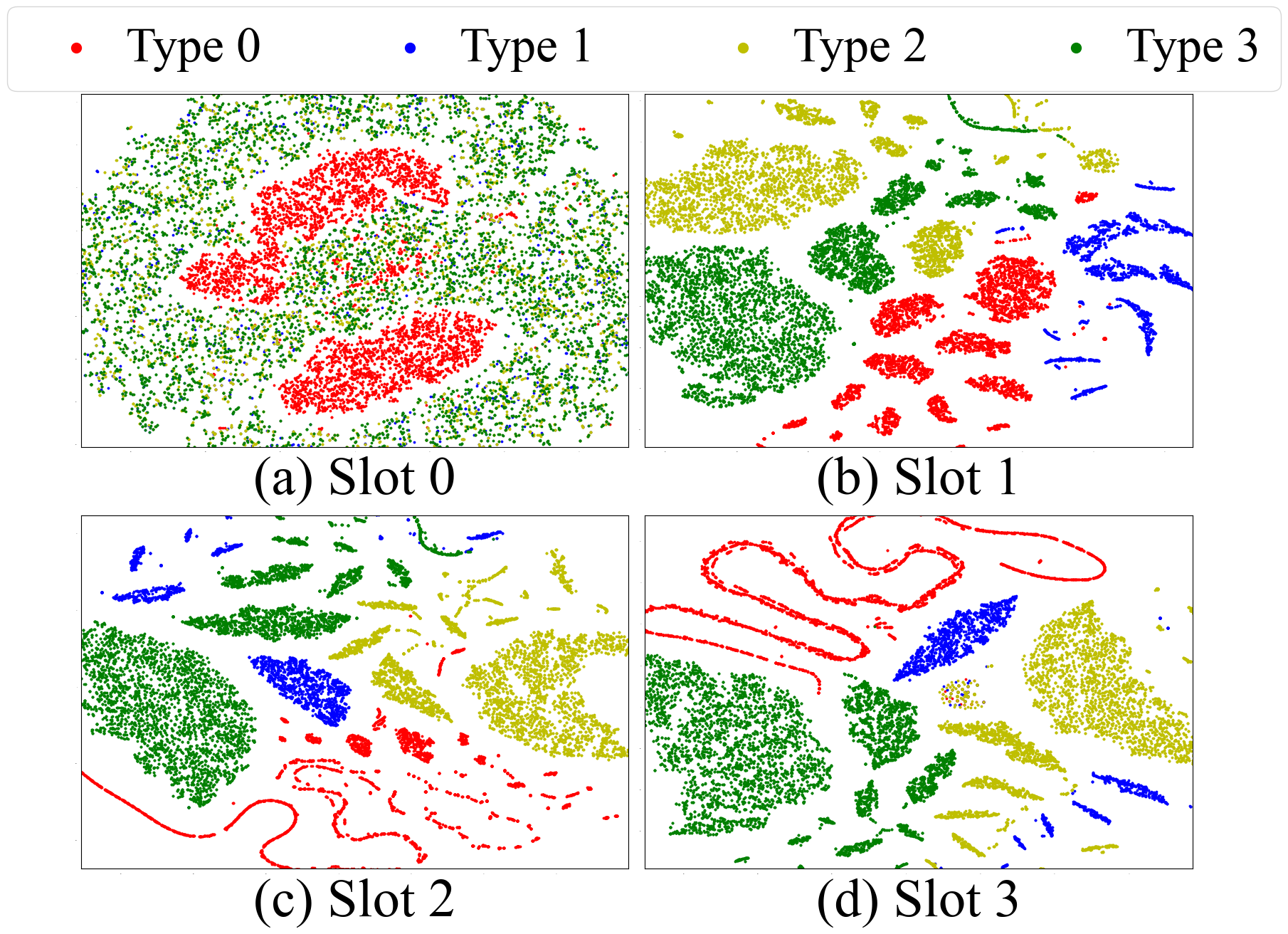
Figure 5: Tsne visualization on all slot representations of $2$-nd SlotGAT layer on IMDB

Slot Visualization. We adopt Tsne (van der Maaten & Hinton, 2008) to visualize the slot representations of SlotGAT. Figure 5 reports the slot visualization of the 2-nd SlotGAT layer on IMDB. Figure 5(a) is the visualization of the 0-th slots (in type-0 feature space) of all nodes with colors representing their own types. Figure 5(b), (c), (d) are the visualization of 1-st, 2-nd, and 3-rd slots of all nodes respectively. First, observe that the 4 slots of a node (for all nodes in a graph) learn radically different representations, as the visualizations in the four figures exhibit different patterns. For instance, in Figure 5(a), 0-th slots can distinguish nodes in type 0 (red) from others, but cannot distinguish nodes of types 1, 2, 3. On the other hand, in Figure 5(b), 1-st slots can distinguish nodes of all types in 0, 1, 2, 3. Similar observations can be made in Figures 5(c) (d). The visualization in Figure 5 validates that SlotGAT is able to learn richer semantics in a finer granularity and also preserve the semantic differences of different node-type feature spaces, which explains the superior performance of SlotGAT. Additional visualization on DBLP is provided in Appendix A.3.

Table 6: Ablation for Slot Attention (Macro-F1/Micro-F1) on node classification. Best is in bold, and runner up is underlined.

	DBLP		IMDB		ACM		PubMed_NC		Freebase
	Macro-F1	Micro-F1	Macro-F1	Micro-F1	Macro-F1	Micro-F1	Macro-F1	Micro-F1	Macro-F1	Micro-F1
SlotGAT	94.95±0.20	95.31±0.19	64.05±0.60	68.54±0.33	93.99±0.23	94.06±0.22	47.79±3.56	53.25±3.40	49.68±1.97	66.83±0.30
SlotGAT (average)	94.52±0.31	94.93±0.25	62.71±1.10	67.56±0.42	93.43±0.50	93.35±0.43	47.18±4.16	52.61±3.23	47.90±1.61	67.01±0.90
SlotGAT (target slot)	87.12±8.44	87.73±7.91	39.35±18.9	48.91±11.2	93.63±1.03	93.50±1.15	44.60±4.14	50.54±4.65	48.77±2.86	66.38±0.50
SlotGAT (last fc)	94.72±0.22	95.11±0.21	63.15±0.53	68.16±0.31	93.91±0.35	93.99±0.35	48.24±5.37	53.72±2.88	51.63±0.75	66.68±0.42

Table 7: Statistical Significance Test between SlotGAT and its variants w.r.t. Micro-F1.

	DBLP	IMDB	ACM	PubMed	Freebase
SlotGAT (average)	0.0090	0.0362	0.0379	0.0226	0.3054
SlotGAT (target slot)	0.0129	0.1014	0.0300	0.0248	0.1988
SlotGAT (last fc)	0.0832	0.6714	0.2840	0.1588	0.2571

Table 8: Statistical Significance Test between SlotGAT and its variants w.r.t. Macro-F1.

	DBLP	IMDB	ACM	PubMed	Freebase
SlotGAT (average)	0.0042	0.0325	0.0359	0.1833	0.2611
SlotGAT (target slot)	0.0304	0.1074	0.0372	0.1984	0.1160
SlotGAT (last fc)	0.0420	0.6952	0.2748	0.9704	0.2114

Statistical Significance Test. In Table 4, we report the p-values of paired t-tests between SlotGAT and the best baseline simpleHGN, w.r.t., micro-F1 and macro-F1 for node classification. In Table 5 we report the p-values on link prediction w.r.t. ROC-AUC and MRR. P-value below 0.05 means statistical significance. Observe that most p-values are below $0.05$ except two p-values, indicating the improvement of SlotGAT over simpleHGN is statistically significant and robust.

Slot Attention Ablation. We ablate the slot attention technique in Section 4.3 that integrates all slots of a node, and compare with other ways, including average (Eq. 9), non-biased fully connected layer (last fc) in Eq. 10, and target slot only (target): $\small\mathbf{h}_{v}^{(L)}=\frac{1}{|\Phi_{target}|}\sum_{t\in\Phi_{target}}\mathbf{h}_{v}^{(L),t}\in^{d_{L}}.$ The results are reported in Table 6. Observe that SlotGAT with slot attention is the best on DBLP, IMDB, and ACM, and is top-2 on PubMed_NC and Freebase. The results validate the effectiveness of slot attention. Moreover, SlotGAT (average) and SlotGAT (target) are not with high performance, indicating that blindly averaging slot representations or only using the target slot are less effective. Moreover, We provide the paired t-test results between SlotGAT and its variants w.r.t. Micro-F1 and Macro-F1 in Table 7 and Table 8 respectively. Combining with the results in Table 6, we have the following observations. (i) On DBLP, IMDB, ACM and PubMed_NC for Micro-F1 (Table 7), the improvement of SlotGAT over SlotGAT(average) and SlotGAT(target slot) is statistically significant, since 7 out of the 8 corresponding p-values are below 0.05, and similar observation can be made on Table 8 for these methods. (ii) As shown in Table 6, SlotGAT(last fc) is comparable to SlotGAT, and thus the corresponding p-values are relatively large in the last rows of Tables 7 and 8. Note that SlotGAT (last fc) is less explainable than SlotGAT with slot attention. (iii) On Freebase, all methods have close F1 scores in Table 6, and thus the p-values are relatively large in the last columns of Tables 7 and 8. These observations, combined with Table 6, validate our statement that SlotGAT with slot attention is the best on DBLP, IMDB, and ACM, and is top-2 on PubMed_NC and Freebase.

Efficiency. Tables 9 and 10 report the training time and inference time of SlotGAT compared with simpleHGN and HGT, two strong baselines. Table 11 reports the peak memory usage. As shown, SlotGAT has moderate training and inference time and slightly higher memory usage to achieve the state-of-the-art effectiveness reported ahead.

Table 9: Training time per epoch (millisecond)

	DBLP	IMDB	ACM	PubMed_NC	Freebase
simpleHGN	76.21	75.57	105.44	170.77	423.32
SlotGAT	230.61	241.36	131.98	520.95	458.23
HGT	741.23	613.12	1097.8	2384.14	3711.24

Table 10: Inference time (millisecond)

	DBLP	IMDB	ACM	PubMed_NC	Freebase
simpleHGN	57.1	54.42	47.16	70.67	175.34
SlotGAT	127.19	119.95	69.1	258.44	231.31
HGT	531.13	410.52	650.12	1818.42	2939.8

Table 11: Peak GPU memory (GB)

	DBLP	IMDB	ACM	PubMed_NC	Freebase
simpleHGN	3.46	3.01	6.32	5.96	7.06
SlotGAT	6.36	5.97	5.5	13.37	9.32
HGT	1.34	1.08	2.02	2.54	6.75

6 Conclusion, Limitation, and Future Work

In this paper, we identify a semantic mixing issue that potentially hampers the performance on heterogeneous graphs. To alleviate the issue, we design SlotGAT with separate message passing processes in slots, one for each node type. In such a way, SlotGAT conducts slot-based message passing. We also design an attention-based aggregation mechanism over all slot representations to conduct effective slot-wise message aggregation per layer. To effectively support downstream tasks, we further develop a slot attention technique. Extensive experiments validate the superiority of SlotGAT.

SlotGAT has factor $|\Phi|$ as a trade-off of efficiency for effectiveness, which is a potential limitation if many node types exist. There are several ways to handle this in the future, e.g., being selective on node types to reduce the number of slots and setting a limit on the dimension of all slots.

Appendix A Appendix

All experiments are conducted on a machine powered by an Intel(R) Xeon(R) E5-2603 v4 @ 1.70GHz CPU, 131GB RAM, and a Nvidia Geforce 3090 Cards with Cuda version 11.3. Source codes of all competitors are obtained from respective authors.

A.1 Dataset Descriptions

For all of the benchmark datasets, one could access them in online platform HGB. In the following, we provide the descriptions of these datasets. The detailed data statistics, including the number of nodes in every type and the number of edges in every type, can be found at https://github.com/scottjiao/SlotGAT_ICML23/data_statistics.txt.

• DBLP is a bibliography website of computer science. There are 4 node types, including authors, papers, terms, and venues, as well as $6$ edge types. The edge types include paper-term, paper-term, paper-venue, paper-author, term-paper, and venue-paper. The target is to predict the class labels of authors. The classes are database, data mining, AI, and information retrieval.

• IMDB is a website about movies. There are 4 node types: movies, directors, actors, and keywords. A movie can have multiple class labels. The $6$ edge types include movie-director, director-movie, movie-actor, actor-movie, movie-keyword, and keyword-movie. There are 5 classes: action, comedy, drama, romance, and thriller. Movies are the targets to classify.

• ACM is a citation network (Wang et al., 2019d), containing node types of authors, papers, terms, and subjects. The edge types include paper-cite-paper, paper-ref-paper, paper-author, author-paper, paper-subject, subject-paper, paper-term, and term-paper. The node classification target is to classify papers into 3 classes: database, wireless communication, and data mining.

• Freebase (Bollacker et al., 2008) is a large knowledge graph with 8 node types, including book, film, music, sports, people, location, organization, and business, and 36 edge types. The target is to classify books in 7 classes: scholarly work, book subject, published work, short story, magazine, newspaper, journal, and poem.

• LastFM  is an online music website. There are 3 node types: user, artist, and tag. And it has $3$ edge types: user-artist , user-user, artist-tag. The link prediction task aims to predict the edges between users and artists.

• PubMed is a biomedical literature library. We use the data constructed by (Yang et al., 2022). The node types are gene, disease, chemical, and species. The $10$ edge types contain gene-and-gene, gene-causing-disease, disease-and-disease, chemical-in-gene, chemical-in-disease, chemical-and-chemical, chemical-in-species, species-with-gene, species-with-disease, and species-and-species. The target of the node classification task is to predict the disease into eight categories with class labels from (Yang et al., 2022). The target of link prediction is to predict the existence of edges between genes and diseases.

Table 12: Data Split of Node Classification Datasets.

	#Nodes	#Training	#Validation	#Testing
DBLP	26,128	974	243	2,840
IMDB	21,420	1,097	274	3,159
ACM	10,942	726	181	2,118
Freebase	180,098	1,909	477	4,446
PubMed_NC	63,109	295	73	86

Table 13: The searched hyper-parameters for SlotGAT with best performances on various datasets.

Datasets	AttDim	lr	wd	dropAttn	droptFeat	featType	hiddenDim	Layers	Epoch	Heads	Decoder	EdgeDim
DBLP	32	1e-4	1e-3	0.5	0.5	1	64	4	300	8	-	64
IMDB	3	1e-4	1e-3	0.2	0.8	1	128	3	300	8	-	64
ACM	32	1e-3	1e-4	0.8	0.8	1	64	2	300	8	-	64
pubmed_NC	3	5e-3	1e-3	0.8	0.2	1	128	2	300	8	-	64
Freebase	8	5e-4	1e-3	0.5	0.5	2	16	2	300	8	-	0
LastFM	64	5e-4	1e-4	0.9	0.2	2	64	8	1000	2	DotProduct	64
pubmed_LP	32	1e-3	1e-4	0.5	0.5	2	64	4	1000	2	DistMult	64

A.2 Node Classification Data Split

Following (Lv et al., 2021), we have the training and validiation ratio 8:2, while keeping fixed testing test, and the statistics of testing data, as well as training and validation data are listed in Table 12.

A.3 Additional Visualization Results

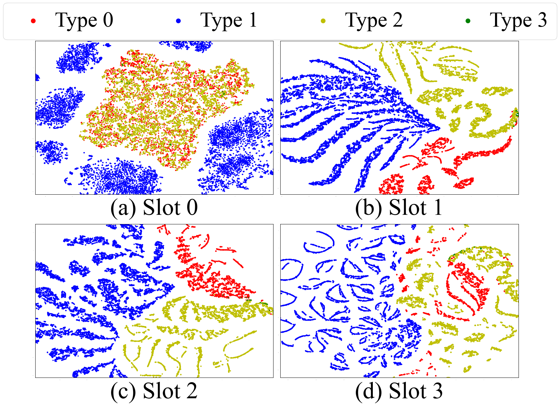
Figure 6: Tsne visualization on all slot representations of $3$-rd SlotGAT layer on DBLP

Figure 6 reports the Tsne visualization on the slot representations of the 3-rd SlotGAT layer on DBLP. In particular, Figure 6(a) is the visualization of the 0-th slots (in type-0 feature space) of all nodes with colors representing their own types, and Figure 5(b), (c), (d) are the visualization of 1-st slots (in type-1 feature space), 2-nd slots (in type-2 feature space), 3-rd slots (in type-3 feature space) of all nodes respectively. First, observe that the 4 slots of a node (for all nodes in a graph) learn very different representations, as the visualizations in the four figures exhibit different patterns. Note that the number of nodes in type 3 is very few compared to other three node types, and thus are nearly invisible in these figures. Therefore, we focus the discussion on nodes of the other three types in red, blue and yellow. In particular, as shown in Figure 6(a), the 0-th slots (in type-0 feature space) are able to distinguish nodes in type 1 (blue) from others, but cannot distinguish nodes of types 0, 2, 3. On the other hand, in Figure 6(b), the 1-st slots (in type-1 feature space) are able to distinguish nodes of different types in 0, 1, 2. Similar observation can be made in Figures 6(c),(d). The visualization in Figure 6 proves that SlotGAT is able to learn richer semantics in finer granularity and also preserve the semantic differences of different node-type feature spaces into different slots. This visualization also provide evidence on the superior performance of SlotGAT.

A.4 Link Prediction Decoders

Given $\mathbf{H}_{v}$ and $\mathbf{H}_{u}$, dot product decoder first computes dot product and then applies a sigmoid activation function: $Decoder(\mathbf{H}_{v},\mathbf{H}_{u})=\sigma(\langle\mathbf{H}_{v},\mathbf{H}_{u}\rangle)$.

DistMult requires a learnable square weight matrix $\mathbf{W}_{\psi(v,u)}\in^{d_{L}\times d_{L}}$ for edge type $\psi(v,u)$.Then a bi-linear form between $\mathbf{H}_{v},\mathbf{H}_{u}$ is calculated as: $Decoder(\mathbf{H}_{v},\mathbf{H}_{u})=\sigma(\mathbf{H}_{v}^{\top}\mathbf{W}_{\psi(v,u)}\mathbf{H}_{u})$. The choice of dot product or DistMult is regarded as a part of hyper-tuning process (Lv et al., 2021).

A.5 Searched Hyper-parameters

To facilitate the re-producibility of this work, we present the searched hyper-parameters of SlotGAT in Table 13 on different datasets. Note that due to the high computational cost in dataset Freebase, we set the dimension $d_{e}=0$ of attention vector for edge types in this dataset, while $d_{e}=64$ in all other datasets. Moreover, three tricks are used in the implementation of SlotGAT as suggested in (Lv et al., 2021): residual connection, attention residual and using hidden embedding in middle layers for link prediction tasks.

A.6 Metrics

Here we illustrate how we compute the four metrics: Macro-F1, Micro-F1, ROC-AUC and MRR.

Macro-F1: The macro F1 score is computed using the average of all the per-class F1 scores. Denote $\text{Precision}_{c}$ as the precision of class $c$, and $\text{Recall}_{c}$ as the recall of class $c$. We have

$$\text{Macro-F1}=\frac{1}{C}\sum_{c\in[C]}\frac{2\text{Precision}_{c}\cdot\text{Recall}_{c}}{\text{Precision}_{c}+\text{Recall}_{c}}.$$ (14)

Micro-F1: The Micro-F1 score directly uses the total precision and recall scores. With the Precision and Recall scores of all nodes regardless of their classes, we have

$$\text{Micro-F1}=\frac{2\text{Precision}\cdot\text{Recall}}{\text{Precision}+\text{Recall}}.$$ (15)

ROC-AUC: The Area Under the Curve (AUC) score is calculated from Receiver Operating Characteristic (ROC). Define the True Positive Rate (TPR) as $\text{TPR}=\frac{\text{TP}}{\text{TP+FN}}$, where TP, FN represent true positive and false negative respectively. The False Positive Rate (FPR) is calculated as $\text{FPR}=\frac{\text{FP}}{\text{FP+TN}}$, where FP, TN represent false positive and true negative respectively. One can see that, TPR and FPR scores vary if we change the classification threshold. One can also prove that, there exists a one-to-one function $f$ such that under every threshold: $f(\text{FPR})=\text{TPR}$. Then the ROC-AUC score is the area under the graph of this function $f$:

$$\text{ROC-AUC}=\int_{x\in[0,1]}f(x).$$ (16)

MRR: Mean reciprocal rank (MRR) is a metric usually used in recommendation system. Here we use it to evaluate performance in link prediction as in (Lv et al., 2021). For each node $v$ involved in concerned edges, i.e., positive and negative edges to be evaluated, one can sort its all related nodes $u$, i.e., connected by these positive or negative nodes, by the similarities of their computed embeddings. Then, denote the minimal rank of the first occurred nodes $u$ connected with positive links $(v,u)\in{\mathcal{E}}_{pos}$ in the above sorted nodes list as $R_{v}$, we have the MRR as the mean of reciprocal of this minimal rank over all the involved nodes $\{(v,u)\in{\mathcal{E}}_{pos}\text{ or }{\mathcal{E}}_{neg}\}$.

A.7 Meta-paths Used in Baselines

We provide the meta-paths used in baselines in Table 14, which are widely adopted in  (Lv et al., 2021; Fu et al., 2020; Wang et al., 2019d).

Table 14: Meta-paths used in our experiments.

Dataset	Meta-paths	Meaning
DBLP	APA, APTPA, APVPA	A: Author, P: Paper, T: Term, V: Venue
IMDB	MDM, MAM, DMD, DMAMD, AMA, AMDMA, MKM	M: Movie, D: Director, A: Actor, K: Keyword
ACM	PAP, PSP, PcPAP, PcPSP, PrPAP, PrPSP, PTP	P: Paper, A: Author, S: Subject, T: Term, c: citation relation, r: reference relation
Freebase	BB, BFB, BLMB, BPB, BPSB, BOFB, BUB	B: Book, F: Film, L: Location, M: Music, P: Person, S: Sport, O: Organization, U: bUsiness
LastFM	UU, UAU, UATAU, AUA, ATA, AUUA	U: User, A: Artist, T: Tag
PubMed	DD, DGGD, DCCD, DSSD	D: Disease, G: Gene, C: Chemical, S: Species

A.8 Proof of Theorem 4.1

Proof.

The indication vector for the $i$-th CC is denoted by $\mathbf{1}^{(i)}\in\mathbb{R}^{n}$. This vector indicates whether a node is in the maximal connected component $CC_{i}$, i.e.,

$$\small\mathbf{1}^{(i)}_{j}=\left\{\begin{array}[]{l}1,v_{j}\in CC_{i}\\ 0,v_{j}\not\in CC_{i}\end{array}\right.$$ (17)

If a graph has no bipartite components, the eigenvalues are all in [0,2) (Chung, 1997). The eigenspace of $L_{rw}$ corresponding to eigenvalue 0 is spanned by $\{\mathbf{1}^{(i)}\}_{i=1}^{k}$ (von Luxburg, 2007). For $\alpha\in(0,1]$, the eigenvalues of $(I-\alpha L_{rw})$ fall into (-1,1], and the eigenspace of eigenvalue 1 is spanned by $\{\mathbf{1}^{(i)}\}_{i=1}^{k}$.

Denote $(I-\alpha L_{rw})=G=P\text{diag}\{\lambda_{1},\lambda_{2},...,\lambda_{n}\}P^{\top}$ as the diagnolization of symetric matrix $G$, where $\lambda_{i}$ is the eigenvalues and the $i$-th column of matrix $P$ is the corresponding eigenvector. We compute

$$[\lim_{\ell\to+\infty}{(I-\alpha L_{rw})}^{\ell}\mathbf{X}^{(t)}]_{i}$$ (18)

$$= [\lim_{\ell\to+\infty}G^{\ell}\mathbf{X}^{(t)}]_{i}$$

$$= [P\text{diag}\{\lim_{\ell\to+\infty}\lambda_{1}^{\ell},\lim_{\ell\to+\infty}\lambda_{2}^{\ell},...,\lim_{\ell\to+\infty}\lambda_{n}^{\ell}\}P^{\top}\mathbf{X}^{(t)}]_{i}$$

Since all eigenvalues $\lambda_{i}\in(-1,1]$, only the eigenvalues equal to one could avoid shrinking to $0$. Thus,

$$[P\text{diag}\{\lim_{\ell\to+\infty}\lambda_{1}^{\ell},\lim_{\ell\to+\infty}\lambda_{2}^{\ell},...,\lim_{\ell\to+\infty}\lambda_{n}^{\ell}\}P^{\top}\mathbf{X}^{(t)}]_{i}$$ (19)

$$= \sum_{j=1}^{n}\sum_{o=1}^{n}(\lim_{\ell\to+\infty}\lambda_{o}^{\ell})P_{io}P_{jo}\mathbf{x}^{(t)}_{j}$$

$$= \sum_{j=1}^{n}\sum_{1\leq o\leq n,\atop\lambda_{o}=1}P_{io}P_{jo}\mathbf{x}^{(t)}_{j}$$

Since the eigenspace of matrix $G$ corresponding to eigenvalue $1$ are spanned by $\{\mathbf{1}^{(i)}\}_{i=1}^{k}$ (von Luxburg, 2007), and all of the eigenvectors within the matrix $P$’s columns are orthogonal to each other, we can see that each column $P_{:,o}$ corresponding to eigenvalue $1$ (the count of this kind of vectors is equal to $k$) will be one of the vectors in the set $\{\frac{1}{\sqrt{|CC_{i}|}}\cdot\mathbf{1}^{(i)}\}_{i=1}^{k}$. These $k$ vectors all have $2$-norm equal to $1$, where $|CC_{i}|$ is the size of the $i$-th CC. Thus if $\lambda_{o}=1$, $P_{:,o}$ is one of the vectors in set $\{\frac{1}{\sqrt{|CC_{i}|}}\mathbf{1}^{(i)}\}_{i=1}^{k}$. Then $P_{io}P_{jo}=\frac{1}{|cc(i)|}\iff v_{j}\in cc(i)$ (node $v_{i}$ and node $v_{j}$ in the same CC), where $|cc(i)|$ is the size of the CC which node $i$ is in, otherwise $P_{io}P_{jo}=0$. Therefore,

$${}_{i}= \sum_{j=1}^{n}\sum_{1\leq o\leq n,\atop\lambda_{o}=1}P_{io}P_{jo}\mathbf{x}^{(t)}_{j}$$ (20)

$$= \sum_{v_{j}\in cc(i)}\frac{1}{|cc(i)|}\mathbf{x}^{(t)}_{j}.$$

Since only nodes with type $t$ have non-zero features, Eq. 20 is re-written as:

$${}_{i}= \sum_{v_{j}\in cc(i)}\frac{1}{|cc(i)|}\mathbf{x}^{(t)}_{j}$$ (21)

$$= \sum_{v_{j}\in cc(i),\atop\phi(v_{j})=t}\frac{1}{|cc(i)|}\mathbf{x}^{(t)}_{j}.$$

∎

References

- Bollacker et al. (2008) Bollacker, K., Evans, C., Paritosh, P., Sturge, T., and Taylor, J. Freebase: a collaboratively created graph database for structuring human knowledge. In SIGMOD’08, pp. 1247–1250, 2008.
- Bruna et al. (2014) Bruna, J., Zaremba, W., Szlam, A., and LeCun, Y. Spectral networks and locally connected networks on graphs. In ICLR’14, 2014.
- Cen et al. (2019) Cen, Y., Zou, X., Zhang, J., Yang, H., Zhou, J., and Tang, J. Representation learning for attributed multiplex heterogeneous network. In KDD’19, pp. 1358–1368, 2019.
- Chen et al. (2020a) Chen, D., Lin, Y., Li, W., Li, P., Zhou, J., and Sun, X. Measuring and relieving the over-smoothing problem for graph neural networks from the topological view. In AAAI, pp. 3438–3445. AAAI Press, 2020a.
- Chen et al. (2020b) Chen, M., Wei, Z., Huang, Z., Ding, B., and Li, Y. Simple and deep graph convolutional networks. In ICML’20, pp. 1725–1735, 2020b.
- Chung (1997) Chung, F. R. Spectral graph theory, volume 92. American Mathematical Soc., 1997.
- Defferrard et al. (2016) Defferrard, M., Bresson, X., and Vandergheynst, P. Convolutional neural networks on graphs with fast localized spectral filtering. In NeurIPS’16, pp. 3837–3845, 2016.
- Dong et al. (2017) Dong, Y., Chawla, N. V., and Swami, A. metapath2vec: Scalable representation learning for heterogeneous networks. In KDD ’17, pp. 135–144. ACM, 2017.
- Fan et al. (2019) Fan, W., Ma, Y., Li, Q., He, Y., Zhao, Y. E., Tang, J., and Yin, D. Graph neural networks for social recommendation. In WWW’19, pp. 417–426, 2019.
- Fout et al. (2017) Fout, A., Byrd, J., Shariat, B., and Ben-Hur, A. Protein interface prediction using graph convolutional networks. In NeurIPS’17, pp. 6530–6539, 2017.
- Fu et al. (2020) Fu, X., Zhang, J., Meng, Z., and King, I. Magnn: metapath aggregated graph neural network for heterogeneous graph embedding. In WWW’20, pp. 2331–2341, 2020.
- Gilmer et al. (2017) Gilmer, J., Schoenholz, S. S., Riley, P. F., Vinyals, O., and Dahl, G. E. Neural message passing for quantum chemistry. In ICML’17, pp. 1263–1272. PMLR, 2017.
- Guo et al. (2019) Guo, S., Lin, Y., Feng, N., Song, C., and Wan, H. Attention based spatial-temporal graph convolutional networks for traffic flow forecasting. In AAAI’19, pp. 922–929, 2019.
- Hamilton et al. (2017) Hamilton, W. L., Ying, Z., and Leskovec, J. Inductive representation learning on large graphs. In NeurIPS’17, pp. 1024–1034, 2017.
- Hong et al. (2020) Hong, H., Guo, H., Lin, Y., Yang, X., Li, Z., and Ye, J. An attention-based graph neural network for heterogeneous structural learning. In AAAI’20, volume 34, pp. 4132–4139, 2020.
- Hu et al. (2020a) Hu, Z., Dong, Y., Wang, K., Chang, K.-W., and Sun, Y. Gpt-gnn: Generative pre-training of graph neural networks. In KDD‘20, pp. 1857–1867, 2020a.
- Hu et al. (2020b) Hu, Z., Dong, Y., Wang, K., and Sun, Y. Heterogeneous graph transformer. In WWW’20, pp. 2704–2710, 2020b.
- Kipf & Welling (2017) Kipf, T. N. and Welling, M. Semi-supervised classification with graph convolutional networks. In ICLR’17, 2017.
- Klicpera et al. (2019) Klicpera, J., Bojchevski, A., and Günnemann, S. Predict then propagate: Graph neural networks meet personalized pagerank. In ICLR’19, 2019.
- Li & Goldwasser (2019) Li, C. and Goldwasser, D. Encoding social information with graph convolutional networks for political perspective detection in news media. In ACL’19, pp. 2594–2604, 2019.
- Li et al. (2018) Li, Q., Han, Z., and Wu, X.-M. Deeper insights into graph convolutional networks for semi-supervised learning. In AAAI’18, volume 32, 2018.
- Liu et al. (2020) Liu, M., Gao, H., and Ji, S. Towards deeper graph neural networks. In KDD’20, pp. 338–348, 2020.
- Lv et al. (2021) Lv, Q., Ding, M., Liu, Q., Chen, Y., Feng, W., He, S., Zhou, C., Jiang, J., Dong, Y., and Tang, J. Are we really making much progress?: Revisiting, benchmarking and refining heterogeneous graph neural networks. In KDD ’21, pp. 1150–1160, 2021.
- Monti et al. (2017) Monti, F., Boscaini, D., Masci, J., Rodolà, E., Svoboda, J., and Bronstein, M. M. Geometric deep learning on graphs and manifolds using mixture model cnns. In CVPR’17, pp. 5425–5434, 2017.
- Qiu et al. (2018) Qiu, J., Tang, J., Ma, H., Dong, Y., Wang, K., and Tang, J. Deepinf: Social influence prediction with deep learning. In KDD’18, pp. 2110–2119, 2018.
- Schlichtkrull et al. (2018) Schlichtkrull, M., Kipf, T. N., Bloem, P., Van Den Berg, R., Titov, I., and Welling, M. Modeling relational data with graph convolutional networks. In ESWC’18, pp. 593–607. Springer, 2018.
- Student (1908) Student. The probable error of a mean. Biometrika, pp. 1–25, 1908.
- van der Maaten & Hinton (2008) van der Maaten, L. and Hinton, G. Visualizing data using t-sne. JMLR’08, 9(86):2579–2605, 2008.
- Velickovic et al. (2018) Velickovic, P., Cucurull, G., Casanova, A., Romero, A., Liò, P., and Bengio, Y. Graph attention networks. In ICLR’18, 2018.
- von Luxburg (2007) von Luxburg, U. A tutorial on spectral clustering. Stat. Comput., 17(4):395–416, 2007.
- Wang et al. (2019a) Wang, H., Zhang, F., Zhang, M., Leskovec, J., Zhao, M., Li, W., and Wang, Z. Knowledge-aware graph neural networks with label smoothness regularization for recommender systems. In KDD’19, pp. 968–977, 2019a.
- Wang et al. (2019b) Wang, H., Zhao, M., Xie, X., Li, W., and Guo, M. Knowledge graph convolutional networks for recommender systems. In WWW’19, pp. 3307–3313, 2019b.
- Wang et al. (2019c) Wang, X., He, X., Cao, Y., Liu, M., and Chua, T.-S. Kgat: Knowledge graph attention network for recommendation. In KDD’19, pp. 950–958, 2019c.
- Wang et al. (2019d) Wang, X., Ji, H., Shi, C., Wang, B., Ye, Y., Cui, P., and Yu, P. S. Heterogeneous graph attention network. In WWW’19, 2019d.
- Wang et al. (2020) Wang, Y., Tang, S., Lei, Y., Song, W., Wang, S., and Zhang, M. Disenhan: Disentangled heterogeneous graph attention network for recommendation. In CIKM ’20, pp. 1605–1614. ACM, 2020.
- Yang et al. (2015) Yang, B., Yih, W., He, X., Gao, J., and Deng, L. Embedding entities and relations for learning and inference in knowledge bases. 2015.
- Yang et al. (2020a) Yang, C., Pal, A., Zhai, A., Pancha, N., Han, J., Rosenberg, C., and Leskovec, J. Multisage: Empowering gcn with contextualized multi-embeddings on web-scale multipartite networks. In KDD’20, pp. 2434–2443, 2020a.
- Yang et al. (2022) Yang, C., Xiao, Y., Zhang, Y., Sun, Y., and Han, J. Heterogeneous network representation learning: A unified framework with survey and benchmark. IEEE Trans. Knowl. Data Eng., 34(10):4854–4873, 2022.
- Yang et al. (2020b) Yang, G., Zhang, X., and Li, Y. Session-based recommendation with graph neural networks for repeat consumption. In ICCPR’20, pp. 519–524, 2020b.
- Yun et al. (2019) Yun, S., Jeong, M., Kim, R., Kang, J., and Kim, H. J. Graph transformer networks. In NeurIPS’19, 2019.
- Zhang et al. (2019) Zhang, C., Song, D., Huang, C., Swami, A., and Chawla, N. V. Heterogeneous graph neural network. In KDD’19, pp. 793–803, 2019.
- Zhao et al. (2022) Zhao, T., Yang, C., Li, Y., Gan, Q., Wang, Z., Liang, F., Zhao, H., Shao, Y., Wang, X., and Shi, C. Space4hgnn: A novel, modularized and reproducible platform to evaluate heterogeneous graph neural network. In SIGIR ’22, pp. 2776–2789, 2022.
- Zhu et al. (2019) Zhu, S., Zhou, C., Pan, S., Zhu, X., and Wang, B. Relation structure-aware heterogeneous graph neural network. In ICDM’19, 2019.