Task-Driven Computational Framework for Simultaneously Optimizing Design and Mounted Pose of Modular Reconfigurable Manipulators

Abstract

Modular reconfigurable manipulators enable quick adaptation and versatility to address different application environments and tailor to the specific requirements of the tasks. Task performance significantly depends on the manipulator’s mounted pose and morphology design, therefore posing the need of methodologies for selecting suitable modular robot configurations and mounted pose that can address the specific task requirements and required performance. Morphological changes in modular robots can be derived through a discrete optimization process involving the selective addition or removal of modules. In contrast, the adjustment of the mounted pose operates within a continuous space, allowing for smooth and precise alterations in both orientation and position. This work introduces a computational framework that simultaneously optimizes modular manipulators’ mounted pose and morphology. The core of the work is that we design a mapping function that implicitly captures the morphological state of manipulators in the continuous space. This transformation function unifies the optimization of mounted pose and morphology within a continuous space. Furthermore, our optimization framework incorporates a array of performance metrics, such as minimum joint effort and maximum manipulability, and considerations for trajectory execution error and physical and safety constraints. To highlight our method’s benefits, we compare it with previous methods that framed such problem as a combinatorial optimization problem and demonstrate its practicality in selecting the modular robot configuration for executing a drilling task with the CONCERT modular robotic platform.

I Introduction

Modular manipulators are an intuitive solution to the increasing need for mass-customized manipulation tasks. Specifically, these manipulators, composed of multiple interchangeable body modules, enable rapid and reversible assembly into various morphologies, i.e., the form and structure of a modular robot can be tailored for specific tasks, with an assembly in a few minutes [1].

Determining the morphology of a modular manipulator entails selecting and arranging various modules to assemble a kinematic structure tailored to the needs of particular tasks. This process demands traversal through the modular combinatorial spaces to identify viable morphologies. However, given the exponential increase in possible permutations from adding new modules, conducting an exhaustive search for the various morphologies becomes impractical. Moreover, for the different morphologies, changing the mounted pose of the manipulator affects both the end-effector’s precision and performance in executing the specified task [2, 3].

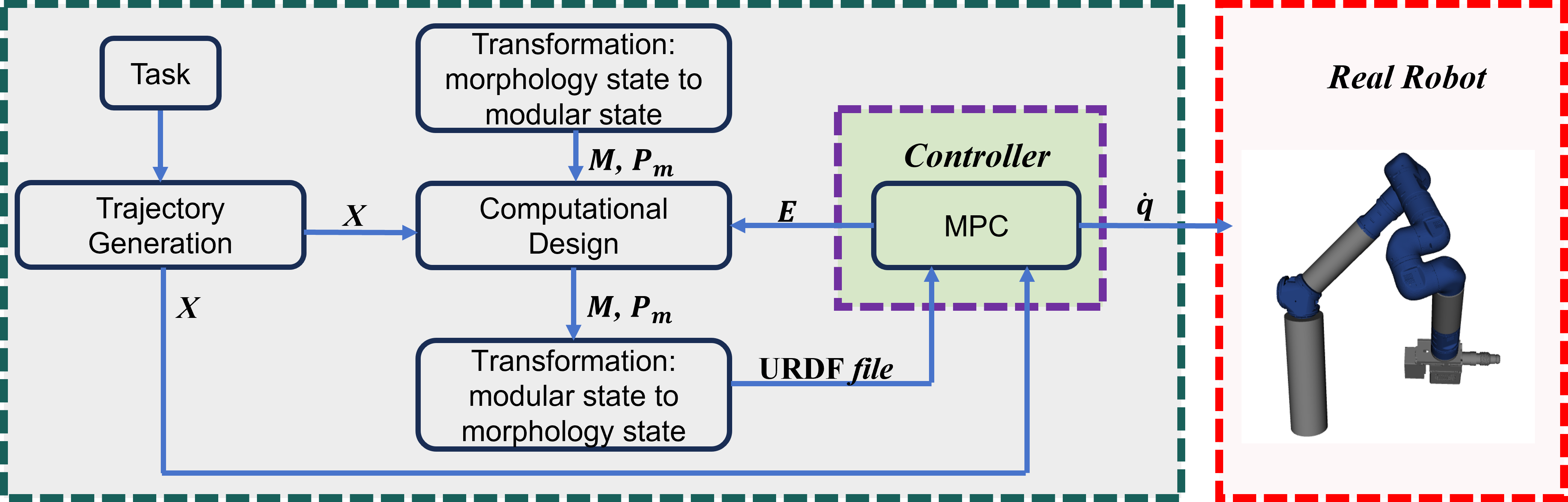
Figure 1: Schematic for the computational framework

Owing to the significant computational effort required to evaluate the vast discrete morphological design space for candidate designs, heuristic-based search methods  [4, 5, 6, 7, 8] have been effectively adapted for modular robot design optimization, streamlining the process by efficiently condensing the combinatorial design space to identify high-performing designs. Meanwhile, optimizing modular robotic manipulators also involves the simultaneous adjustment of the robot’s mounted pose due to its significant impact on the morphological configuration performance. The optimization problem’s complexity escalates when it includes the simultaneous optimization of the robot’s morphology within a discontinuous design space and its mounted pose within a continuous Cartesian space, presenting the challenge of navigating two fundamentally different optimization spaces concurrently. The previous study in [5] addresses this challenge by discretizing the mounted pose into various states, thereby converting the optimization of the mounted pose into a selection process. This method still approaches the simultaneous optimization of mounted pose and morphology as a combinatorial optimization problem.

In this work, we introduce a computational framework for simultaneously optimizing the physical morphology and the mounted pose of modular manipulators, ensuring the optimized result is specifically fit for the given tasks. Unlike the approach in the previous work  [5], our method incorporates the development of a mapping function that implicitly represents the manipulator’s morphology, facilitating the transition of the manipulator’s discontinuous morphological states into a continuous domain. We then apply the sample-efficient Covariance Matrix Adaptation Evolutionary Strategy (CMA-ES) [9] to efficiently search for high-performance solutions within this new framework. Importantly, the mapping function draws inspiration from Natural Language Processing (NLP), since we transform the robot discrete morphology state into a continuous spectrum by assigning variably continuous state variables to each module, a concept parallel but not identical to NLP’s context-driven word selection probabilities [10, 11].

Additionally, we integrate application-specific constraints, such as dynamic boundaries and collision avoidance, to ensure the manipulator’s practical applicability. Moreover, joint space optimization objectives are also considered to refine the optimal results for varying demands of different application scenarios. Particularly in field environments where battery conservation is critical, selecting a robot morphology that minimizes effort is advantageous. On the other hand, in situations where energy consumption is not a primary concern, opting for a morphology that maximizes manipulability may be more beneficial, especially to address challenges related to singularity.

In this framework, manipulation tasks were defined as trajectories in Cartesian space, consisting of a series of desired end-effector poses. We utilize Model Predictive Control (MPC) [12] to control the robot to execute the specified trajectory. The execution’s performance, assessed through designated evaluation metrics, is then leveraged to evaluate different morphologies and mounted pose. Additionally, MPC is able to be applied to control the actual robot in real experiments across varied morphologies. The diagram of our computational framework is shown in Fig.1. The main contributions of this work include:

(i) The mapping function was designed to transform the optimization variables for the manipulator’s morphology and mounted pose both into continuous ones, enabling their simultaneous optimization within a continuous space. We compare it with genetic algorithms(GAs) to show the advantage of our method, which is commonly used to address combinatorial optimization problems.

(ii) A two-level optimization framework was proposed, first ensuring task feasibility through considerations of task executing accuracy, collision avoidance and dynamic boundaries. Then, the framework optimizes performance by maximizing manipulability or minimizing joint effort, further refining the optimal results. We analyze the optimal results by considering various objective functions to demonstrate the effectiveness of our method.

(iii) In our real-world experiments, the CONCERT mobile modular manipulator equipped with a 10kg drilling end-effector continuously is able to executed drilling tasks at various locations. Despite the heavy payload in executing such tasks and two drilling points close to the base link’s horizontal level, the computational results still ensure collision-free with the mounted platform and satisfy dynamic constraints of the robot.

II Related Work

Since the design spaces of modular manipulators are discontinuous, most related research focuses on addressing morphology optimization as a combinatorial optimization problem. This approach needs an exhaustive exploration of the design space to identify the optimal morphology of the modular manipulator. One effective exploration method is to enumerate all possible morphologies of the modular manipulator, as discussed in studies by [13, 14, 6, 15]. This method ensures comprehensive coverage in the search process. However, the enumeration approach demands significant computational resources due to the large number of potential morphologies that need to be explored. To reduce this computational load, the studies in [13, 14, 6, 15] introduced incidence metrics to simply the enumeration’s search space, making it more efficient for practical application. However, this improved efficiency might result in less comprehensive design space exploration.

Another method utilizes population-based stochastic optimization algorithms to address the combinatorial optimization problem in exploring the morphology of modular manipulators. Specifically, genetic algorithms [4, 7, 5, 6] are employed to maintain and update a population of potential solutions. This approach includes processes such as mutation, crossover, evaluation, and selection, all aimed at identifying high-quality candidate individuals within the population. Compared to the enumeration approach, these methods can be more efficient. However, they are sensitive to parameters like population size, mutation rates, and crossover rates. Additionally, there is limited evidence to demonstrate their convergence to global or even local minima [16]. A further method for optimizing the modular manipulators’ morphology employs heuristic-based search strategies. This approach requires mapping the design space onto a search graph and conducting evolutionary searches within this search graph [17, 8, 18]. The main challenge for the heuristic-based search method lies in finding an effective mapping function and developing a practical heuristic function to guide the search. The work in [17] introduced the approach inspired by the A* algorithm, which formulated the design optimization as a shortest path-finding problem with a predefined heuristics function. Meanwhile, the work [8, 18] proposed to iteratively learn heuristic functions from evaluated design’s results with different given tasks. The latter method simplifies the heuristic design process and demonstrates the potential for broader application of modular robots in various environments.

The design automation methods previously discussed are typically addressed using approaches related to combinatorial optimization due to the non-continuous nature of the design space. However, recent work by [19] proposed to employ the Variational Autoencoder (VAE) network to map the discontinuous design space into a continuous latent space. This transformation allows the design optimization problem to be viewed as a continuous black-box optimization problem, potentially enhancing search efficiency compared to using related methods in combinatorial optimization. Nevertheless, the training of the VAE presents a significant challenge due to the necessity for high-quality datasets. The approach described in [19] involves collecting data based on a pre-trained model. However, ensuring the dataset’s quality remains challenging without the pre-trained models [19].

III Preliminaries

III-A Hardware Description

This subsection briefly delineates the hardware components for the modular reconfigurable manipulators. The modular manipulator system is comprised of several pre-designed body modules; each module can be interchangeably connected with another. These body modules are classified into two principal categories: joint and passive.

(i) Joint Modules: The joint modules are categorized into two distinct types: ”straight” and ”elbow.” The straight-type joint modules are actuated along the common central normal to the modular input and output flange interfaces. Conversely, the elbow-type joint modules pivot around a central axis perpendicular to the common central normal. (ii) Passive Link Modules: In contrast to their active counterparts, passive modules are devoid of internal motors and are available in both straight and elbow configurations. The straight-type passive modules are further differentiated by their lengths, including 0.3m, 0.4m, and 0.6m passive link modules.

The modular manipulator is mounted on a mobile platform, which can move to any desired pose within the given environment. For detailed information on the hardware components and the types of modules, readers can refer to [1] for details on our first-generation modular robot, and to Fig. 2(right) for specifics.

III-B Controller

The task to be executed by the modular manipulator is defined as the manipulator end-effector’s desired trajectory. For this purpose, we define the internal model state $\bm{X}$ as follows: $\bm{X}:=[\bm{p}\ \ \bm{o}\ \ \bm{\dot{p}}\ \ \bm{\omega}]^{T}\in\mathbb{R}^{13},$ where $\bm{p}\in\mathbb{R}^{3}$ and $\bm{\dot{p}}\in\mathbb{R}^{3}$ denote the position and linear velocity of the robot’s end-effector in the world frame $\{\bm{W}\}$, respectively. The quaternion $\bm{o}=[\eta,\bm{\epsilon}]\in\mathbb{R}^{4}$ represents the end-effector’s orientation relative to $\{\bm{W}\}$, with $\|\bm{o}\|=1$, where $\eta=o_{w}$ and $\bm{\epsilon}=[o_{x},o_{y},o_{z}]^{T}$. $\bm{\omega}\in\mathbb{R}^{3}$ represents the end-effector’s angular velocity relative to $\{\bm{W}\}$. We them employ MPC as the controller for the modular manipulator. Using the kinematic model, we relate joint velocities $\bm{\dot{q}}$ to the end-effector velocity $\bm{v}_{e}$ via the Jacobian matrix $\bm{J}$, expressed as $\bm{J\dot{q}}=\bm{v}_{e}$. The end-effector’s acceleration is calculated using $\bm{\dot{J}\dot{q}}+\bm{J\ddot{q}}=\bm{\dot{v}}_{e}$. According to the kinematics of the manipulator, the discretized state-space equation, following Forward Euler integration with step size $dt$, is:

$$\bm{X_{k+1}}=\left[\begin{array}[]{c}\bm{p_{k}}+\bm{\dot{p}_{k}}dt\\ \bm{o_{k}}+\bm{o_{k}}\otimes[0,\bm{\omega_{k}}/2]^{T}dt\\ \bm{v_{k}}+\bm{\dot{J}_{k}\dot{q}_{k}}dt+\bm{J_{k}}(\bm{\dot{q}_{k}}-\bm{\dot{q}_{k-1}})\\ \bm{\omega_{k}}+\bm{\dot{J}_{k}\dot{q}_{k}}dt+\bm{J_{k}}(\bm{\dot{q}_{k}}-\bm{\dot{q}_{k-1}})\end{array}\right]$$ (1)

where $k$ represents the node index of the MPC’s prediction horizon. The MPC ensures the task execution within physical limits:

$$\min_{\bm{u}}\sum_{k=1}^{N_{h}}\bigg{(} \lVert\bm{X}(k+1)-\bm{X}_{\text{ref}}(k+1)\rVert_{{\textbf{Q}}_{k}}+\lVert\bm{u}(k)\rVert_{{\textbf{P}}_{k}}\bigg{)}$$ (2)

state-space equation

joint constraints

The solve results $\bm{u}$ can be used for controlling the real robot. For more details, readers can refer to [12].

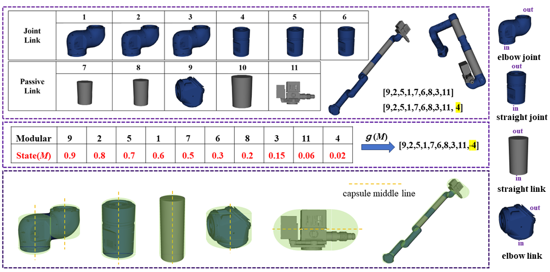
Figure 2: Top left: Encoding of modules by numbers, illustrated with a morphology state example. Middle left: An example of mapping modular states to morphology, where the red word indicates the state variable for different modules. Among them, the 9th module’s state variable is the highest, followed by the 2nd module’s state variable as the second highest. Bottom left: Collision model representation. Right: Types of modules with ”in” indicating connection from the previous module and ”out” showing the connection channel for subsequent modules.

IV Morphology and Mounted Pose Co-Optimization

IV-A Manipulator Morphology Representation

The selection and assembly of diverse modules in various sequences lead to different final morphology for the robot. To accurately represent the morphology of the modular manipulator, we devised an encoder method for the various modules. Assuming our system comprises $m$ modules, each module is assigned a unique numerical identifier. These identifiers are allocated from 1 to $m$, where each number uniquely represents a module. The identified end-effector number is also designated as $m+1$. In cases where multiple units of the same module type are present, each unit is assigned a unique numerical code to differentiate it, even though they are the same. This approach of unique identification eliminates the need for imposing numerical constraints on module quantities in subsequent optimization problems. Since the modular manipulator is structured in series, the morphology of the manipulator can be represented as a vector $\bm{C}_{v}$, known as the morphology state, where $n$ represents the vector’s dimension and the total number of modules used. To clarify the relationship between the actual morphology of the robot and the represented morphology state vector $\bm{C}_{v}$, we provide the following details:

(i): In the morphology vector $\bm{C}_{v}$, the value at each position directly corresponds to the module assembled in that order. Specifically, the first element in this vector represents the first module in the assembly sequence, the second element represents the second module, and so on.

(ii): The total number of the modules $m+1$ can be predetermined. This information allows us to define the maximum dimension of the morphology vector $\bm{C}_{v}\in\mathbb{R}^{n}$. The number of modules used in the manipulator should be less than or equal to $m+1$(the total number of available modules), i.e., $n\leq m+1$.

(iii): The concept of the End of Manipulator (EoM) is introduced, represented by the m+1 module, and serves as the end-effector of the manipulator. The EoM module in the sequence also signifies the completion of the assembly. Therefore, any modules after the EoM module are not considered part of the connected manipulator’s morphology.

This representation method is similar to sentence representation in NLP, wherein the concept of EoM parallels the End Of Sentence (EoS) [10] marker in NLP. In NLP, words following the EoS are not analyzed, and similarly, in the proposed modular robot representation, modules listed after the EoM are not to be assembled. To further illustrate this method with an example, assuming that there are 10 distinct modules ($m=10$), the end-effector module is numbered as $m+1=11$. In this case, the modular manipulator with a morphology state represented by the vector $[9,2,5,1,7,6,8,3,11,4]$ is effectively equivalent to a morphology represented by $[9,2,5,1,7,6,8,3,11]$, since any modules listed after the 11th EoM in the sequence are not considered for assembly with the preceding modules. In other words, if the framework generates two distinct morphological states, such as $[9,2,5,1,7,6,8,3,11,4]$ and $[9,2,5,1,7,6,8,3,11]$, despite the differences in their lengths, module $4$—positioned after the EoM, module $11$—will not be considered for inclusion as one of the modules in the final manipulator morphology. The example of the manipulator’s morphology state is showed in Fig. 2.

IV-B Mapping Function for Morphology Representation

We introduce a mapping function $g(\bm{.})$, designed to transform this discrete morphology state into a continuous module state $\bm{M}\in R^{m+1}$. The mapping function $g(\bm{.})$ in our computational framework draws an intriguing parallel to the concept of word generation probabilities in NLP. In NLP, each word in a sentence has a certain probability of being generated or selected, influenced by the context set by preceding words. This probabilistic approach underscores that word selection is not merely a discrete choice but is guided by continuously varying probabilities [10, 11]. Similarly, our framework assigns each modular component a state variable that varies continuously. This way, the dimension of $\bm{M}\in\mathbb{R}^{m+1}$ is fixed, equaling the total number of modules ($m+1$), where $m+1$ includes the all body modules and the end-effector of the modular. The first element in $\bm{M}$ represents the state of the module with the encoded number $1$, the second element corresponds to the module with the encoded number $2$, and so on. By implementing the mapping function as $\bm{C}_{v}=g(\bm{M})$, the encoded results of each module’s state in $\bm{M}$ implicitly represent the robot’s morphology state $\bm{C}_{v}$. An example is illustrated in the middle of Fig. 2, where each module exhibits different states. These states can implicitly represent the manipulator’s morphology according to the mapping function.

With different states of various modules, the mapping function $g(\bm{.})$ selects and assembles modules in descending order based on their state variable values. It is noted that if the given states of modules are same, then a random method will be employed to sort the modules with the same state, ensuring each module with the same state has an equal probability of being sorted first. The module with the highest value is placed first, continuing until the module with the lowest value is last. This order forms the morphology state vector $\bm{C}_{v}$. This function enables the selection and arrangement of modules according to their state variable values, mirroring the probabilistic selection of words in NLP to form coherent sentences. Thus, our method evolves from a conventional discrete module selection to one influenced by a continuum of values akin to the spectrum of probabilities in NLP word selection.

IV-C Morphology and Mounted Pose Optimization

The optimization objective is to concurrently optimize both the morphology state $\bm{C}_{v}$ and the mounted pose state $\bm{P}_{m}$ of the modular manipulator. The morphology state $\bm{C}_{v}$ is inherently discontinuous, whereas the space for the robot’s mounted pose $\bm{P}_{m}$ is continuous. Here, $\bm{P}_{m}=[x,y,\theta]\in\mathbb{R}^{3}$ represents the mounted pose, where $x$, $y$, and $\theta$ denote the position on the $x$ and $y$ axes and the orientation in the yaw direction in the world frame $\{W\}$ , respectively. The mapping function introduced in the last section transforms the robot’s discontinuous morphological state into a continuous state. Consequently, the problem of optimizing the morphology state $\bm{C}_{v}$ is reframed as optimizing the module state $\bm{M}$. The mapping function ensures that both the morphology $\bm{M}$ and the mounted pose $\bm{P}_{m}$ are in a continuous space.

The optimization focuses on refining two optimal states, including modular state $\bm{M}$ and its mounted pose $\bm{P}_{m}$. The objective is to derive these states to achieve more accurate reference trajectory tracking while considering the given optimization function. For the control policy, regardless of the varying morphologies and mounted pose, all manipulators in this study are controlled using MPC. This controller is designed to optimize the joint states of the manipulator, represented as $\bm{q}\in\mathbb{R}^{d}$, to track the reference trajectory. Here, $d$ is the DoFs of the manipulator. In addition to the tracking error objective, the optimization function must include two constraints: the robot must satisfy dynamic constraints and generate collision-free motion.

IV-C1 Dynamic Constraints

The complete dynamics equation for the manipulator can be expressed as:

$$\bm{M}(\mathbf{q})\ddot{\mathbf{q}}+\mathbf{B}(\mathbf{q},\dot{\mathbf{q}})\dot{\mathbf{q}}+\mathbf{g}(\mathbf{q})+\mathbf{J}^{T}(\mathbf{q})\mathbf{F}_{ext}=\bm{\tau}$$ (3)

In this equation: $\bm{M}(\mathbf{q})$ represents the mass (or inertia) matrix, which depends on the joint positions $\mathbf{q}$;$\ddot{\mathbf{q}}$ is the joint acceleration; $\mathbf{B}(\mathbf{q},\dot{\mathbf{q}})$ is a vector function that includes Coriolis and centrifugal forces; $\dot{\mathbf{q}}$ denotes the joint velocity; $\mathbf{g}(\mathbf{q})$ represents the torque or force due to gravity; $\mathbf{\bm{\tau}}$ is the torque applied to the joints; $\mathbf{J}^{T}(\mathbf{q})$ is the transpose of the Jacobian matrix; $\mathbf{F}_{ext}$ is the vector of external forces acting on the manipulator. For the dynamic constraints of the manipulator, every joint of the manipulator must ensure $||\mathbf{\tau}_{i}||<\mathbf{\tau}_{\text{max}}$ with $i$ represent the $i$-th joint of the manipulator.

IV-C2 Collision-Free Constraints

To efficiently detect collision between the manipulator with various morphologies and the environment, each module is approximated as a capsule(Fig. 2). With these predefined capsule dimensions and parameters, we can assess collisions between each manipulator module and environmental obstacles, which facilitates the detection of collisions for the entire manipulator in different morphologies. Additionally, the position of each module within the environment can be determined through forward kinematics. To calculate the distance between a capsule and an environmental obstacle, we measure the distance between the capsule and the obstacle by using the FCL [20]. The collision constraints are formulated as follows:

$$\text{C}(\bm{p}_{r})\geq d_{\text{safe}},\ \forall\bm{p}_{r}\in\text{Robot},$$ (4)

where $\bm{p}_{r}$ represents the point on the robot, and $d_{\text{safe}}$ is the minimum allowable distance between robot and obstacles.

IV-C3 Joint Space Optimization

In addition to the primary objectives, we also consider an optimized state by considering the ’soft objective.’ We design two distinct objective functions: one focused on minimizing effort and the other on maximizing manipulability. This dual-focused approach enables us to optimize for the most appropriate result based on specific operational requirements. For the minimizing effort function, we can write as:

$$\text{min}\ \ F_{\text{eff}}=\frac{1}{N}\sum_{i=1}^{N}\sum_{j=1}^{d}|\tau(q_{i,j})|$$ (5)

In this equation, $\tau()$ represents the torque at the joint. The specific process of calculating this torque can be further referenced in [1]. The second metric aims at maximizing manipulability, which can be expressed as:

$$\text{max}\ \ M_{\text{man}}=\frac{1}{N}\sum_{i=1}^{N}{\text{det}(\bm{J}(\bm{q}_{i})\bm{J}(\bm{q}_{i})^{T})}$$ (6)

where $\bm{J}(\bm{q})$ is the Jacobian matrix of the manipulator at a given configuration $\bm{q}$ at the $i$-th control loop, $N$ and $d$ represent the total number of control loops of the controller and the DoFs, respectively.

IV-C4 Optimization Formulation

The primary objective for the manipulator is to proficiently execute assigned tasks while adhering to the given constraints. To ensure both the feasibility of the trajectory and the robot’s safety, it is imperative that the tracking error remains below a specified threshold. Additionally, the robot must satisfy dynamic constraints and avoid collisions with the obstacles. The formulation of the optimization problem, which encapsulates these requirements, can be expressed as follows:

$$\underset{g(\bm{M}),\textbf{P}_{m}}{\text{minimum}} X_{e}=-we^{-w_{f}F_{\text{eff}}+w_{m}M_{\text{man}}}$$ (7)

subject to $$\bm{q}_{i}\in[\bm{\underline{q}},\ \ \bm{\overline{q}}],$$

$$||FK(\bm{M},\bm{P}_{m},\bm{q}_{i})\bm{T}_{d,i}^{-1}||^{2}\leq\xi,\ \forall i,$$

$$\text{C}(\bm{p}_{r})\geq d_{\text{safe}},\ \forall\bm{p}_{r}\in\text{Robot},$$

$$\forall i\ \ ||\tau_{i}(\mathbf{q}_{i},\dot{\mathbf{q}}_{i},\ddot{\mathbf{q}}_{i})||<\mathbf{\tau}_{\text{max,i}},$$

where $w$, ${w}_{f}$ and ${w}_{m}$ represent the weight for optimization objective, optimizing minimum joint effort and maximum manipulability, respectively. The variables $\bm{\underline{q}}$ and $\bm{\overline{q}}$ denote the lower and upper bounds of the robot’s joint state, respectively, namely the manipulator joint limits. The $FK(\bm{.})$ represents the forward kinematics results of the manipulator, with the output being the manipulator’s end-effector state, $\bm{T}_{d,i}$ represents the desired state of the end-effector at $i$-th control loop, and $\xi$ represents the threshold for the tracking error. This final optimization result includes the modular state $\bm{M}$ and mounted pose $\bm{P}_{m}$, thereby fulfilling the requirements of the task. Then, we rewrite the optimization in a non-constrained formulation. The optimization function considers five key aspects: manipulator’s manipulability, joint effort, tracking error, collision constraints penalty, and dynamic constraints penalty. The primary objective of this optimization formulation is to minimize the tracking error. If dynamic or collision constraints are not satisfied, a significant penalty is imposed on the optimization function. Once the tracking error is diminished to below a specified threshold $\xi$, the optimization function then shifts focus to joint space for minimize joint effort or maximum manipulability. The objective function is articulated as follows:

$$\underset{\bm{M},\bm{P}_{m}}{\text{minimize}}\ \ E=\underbrace{E_{\text{track}}+E_{\text{collision}}+E_{\text{dynamic}}}_{E_{\text{sum}}}-$$ (8)

$$\quad\begin{cases}we^{-w_{f}F_{\text{eff}}+w_{m}M_{\text{man}}},&\text{if }E_{\text{sum}}<\xi\\ 0,&\text{otherwise.}\end{cases}$$

where

$$E_{\text{track}}(\bm{M},\bm{P}_{m},\bm{q})=\frac{1}{N}\sum_{i=1}^{N}||FK(\bm{M},\bm{P}_{m},\bm{q}_{i})\bm{T}_{d,i}^{-1}||^{2},$$ (9)

$$E_{\text{collision}}(\bm{M},\bm{P}_{m},\bm{q})=\begin{cases}${10}^{10}$,&\text{collision detected}\\ 0,&\text{otherwise},\end{cases}$$ (10)

$$E_{\text{dynamic}}(\bm{M},\bm{P}_{m},\bm{q})=\begin{cases}${10}^{10}$,&\text{dynamic constraints violated}\\ 0,&\text{otherwise}.\end{cases}$$ (11)

$$E_{\text{sum}}=E_{\text{track}}+E_{\text{collision}}+E_{\text{dynamic}}$$ (12)

The function is structured hierarchically. Only when the tracking error is smaller than the given threshold, while adhering to collision and dynamic constraints, the optimization process proceed to consider further the optimization for maximum manipulability and minimum joints’ effort. This layered approach ensures that fundamental performance metrics are prioritized before advancing to refine additional aspects of the robot’s functionality. To address this optimization problem, we employ the CMA-ES as the gradient-free optimizer, considering both the optimal state’s continuous space and the object’s constraints. The optimal results from Eq. 8 include the modular state $\bm{M}$, and the mounted pose $\bm{P}_{m}$. The final morphology state can be calculated using the mapping function as $\bm{C}_{v}=g(\bm{M})$.

V Experiments and Evaluations

V-A Experimental Setup

For the parameters in the CMA-ES algorithm, we set the maximum number of generations to 100, and the maximum number of populations in each evaluation loop is set to 20, with sigma being 0.25. The evaluation process is executed on multi-process CPUs. Regarding the parameters in the controller, The tracking gains for position and orientation in MPC are set at $10$ and $4$ in $\bm{Q}_{k}$. The gains for the regularizer $\bm{P}_{k}$ in the controller are set at 0.0001, horizon set at 10,and the control frequency is 100Hz(dt = 0.01). The controller’s parameters remain consistent across different morphologies of the robot. Meanwhile, the maximum continues joint torque for modules $1$, $2$, $4$, and $5$ is set at 120 Nm, whereas for modules $3$ and $6$, it is 200 Nm. The joint position limits for each module range from -2.7 to 2.7 radians and the maximum joint velocity is capped at 2.0 rad/s. The optimization gains $w$ in Eq. 8 was set to 10, and tracking threshold $\xi$ was set to 0.001. Additionally, with a total of 10 modules available, there are approximately $10!=3,628,800$ different morphologies that can be constructed. We have a mobile platform on which the modular manipulator can be installed. This platform can be positioned in various pose within the environment.

V-B Task Description

We designed one specific task to demonstrate the effectiveness of our proposed framework. This task involves using an end-effector drilling tool for drilling into walls, a common task in building scenarios. The task requires drilling six points on the vertical wall with the same orientation. During the drilling process, the end-effector requires maintaining an orientation perpendicular to the wall while orientation in the $z$-direction, relative to the end-effector’s framework along the axis of the drill-bit is less critical and can be overlooked. There are two main obstacles in the environment: the mobile platform and the walls within the environment. However, the collision problem can be ignored between the robot and the walls during the drilling process. During the drilling process, it is also necessary to consider the contact force exerted on the end-effector between the robot and the wall.

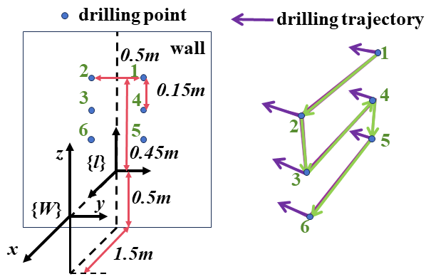
Figure 3: Arrangement of drilling points relative to the wall and world frame.

The drilling points are specified relative to the world frame $\{W\}$. The height between the base link and the ground is 0.5m (the height of the mobile platform). The coordinates of the drilling points are as follows: at a distance of 1.5 m to the world frame’s origin on the $x$-direction, the points alternate along the $y$-axis at intervals of 0.15 m forward and backward, with $z$-axis values descending in increments of 0.15 m from a starting height of 0.45 m. The drilling sequence corresponding locations are given by the coordinates $[-1.5,0.15,0.45]$, $[-1.5,-0.15,0.45]$, $[-1.5,-0.15,0.30]$, $[-1.5,0.15,0.30]$, $[-1.5,0.15,0.15]$, and $[-1.5,-0.15,0.15]$ with respect to the world frame $\{W\}$. Fig.3 on the left illustrates the arrangement of the drilling points relative to the wall and the world frame. The dashed lines indicate the horizontal distances from the wall to the drilling points, while the solid lines with arrows represent the axes of the wall coordinate frame $\{l\}$ and the world frame $\{W\}$. Fig.3 on the right shows the designated 3D trajectory for the drilling task; the purple line signifies the drilling trajectory, with a depth of 0.1 meter, and the green line illustrates the trajectory for moving the robot from one point to the next.

V-C Comparison Study

We conduct a comparative analysis with the baseline algorithms to demonstrate the efficiency and advantages of our proposed computational method. The weights assigned to the objectives of manipulability and effort were set at 1 and 0.01, respectively, indicating that [$w_{m}$, $w_{f}$] = [1.00, 0.01]. The baseline methodology involves adapting GAs, with the implementation following the approach described in [5]. This approach discretizes the mounted pose into various states, effectively transforming the state of the mounted pose into a discretized format. This enables the simultaneous optimization of the robot’s mounted pose and morphology while still addressing it as a combinatorial optimization problem. In our evaluation’s context, we situate the scenario within a work-cell where the limitation of the robot’s base position is $1.2m\times 0.6m$, and rotationally in the world frame’s $z$-axis, ranging from $\pi$ to $-\pi$, a setup that mirrors the design outlined in [5]. In alignment with [5], the position discretization step was set at $0.2m$ and the angle discretization step at $\frac{\pi}{2}$ rad. Consequently, the established mounted position yields 5 and 3 discrete states along the $x$ and $y$ axes, respectively, and 4 possible rotational states along the $z$-axis.

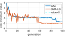
(a) 20 population

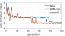
(b) 40 population

Figure 4: Minimum cost evolution over generations with different population.

In GAs setup, the mutation probability was set at 0.5, and the crossover probability was set at 0.1 with the 100 generations. For the first comparison group, we aligned the population size for each generation at 20, mirroring the settings used in CMA-ES. In the second comparison group, we adjusted the population size for both GAs and CMA-ES to 40, consistent with the parameters set in [5].

To execute the specified tasks, we first tackle the inverse kinematics (IK) challenge to pinpoint the trajectory’s initial desired point, setting this as the MPC’s initial joint state. We then simulate five distinct IK solutions as initial configurations for the joint setup to enable a productive warm start for the MPC, evaluating their performance in the process. The most efficient initial configuration state and its performance evaluation are recorded to optimize the morphology and mounted pose. These warm-start findings are also valuable for application in real-world experimental conditions.

Fig. 4 depicts the minimum value achieved by each generation when employing GAs and CMA-ES for the optimization with the different given population. It is important to note that a cost value smaller than zero indicates that the task at the first level was successfully accomplished. It means the tracking error is smaller than the given threshold while also adhering to the dynamic and collision constraints. Compared to GAs, our computational methods demonstrate superior performance in both convergence speed and the quality of solutions for the specified cost function, regardless of the population size, which is reflected in consistently lower fitness values in the figure. Notably, this improvement occurs even though the population size in the CMA-ES is 20 in every generation, which is smaller than the population size used in our previous work [5]. To be honest, the rationale behind setting discrete parameters for comparative analysis is to align with the setting presented in the paper [5]. Therefore, we adopt the parameterization outlined in this reference. In real-world applications, finer discretization of our space could be considered to enhance the quality of optimization results. However, this refinement tends to decelerate the convergence speed of GAs by broadening the spectrum of choices, thereby complicating the selection process. Moreover, it is note that, in practical scenarios, the potential for discretization is essentially boundless.

V-D Evaluations with Different Optimization Objectives

M	$\textbf{{P}}_{m}$	$w_{m}$, $w_{f}$	$E_{\text{track}}$	$M_{\text{man}}$	$F_{\text{eff}}$
C-1	[-0.15, 0.21, 1.57]	1, 0.01	$3.6\text{\times}{10}^{-5}$	0.41	198.7
C-2	[0.29, -0.03, 2.2]	1, 0.00	$1.06\text{\times}{10}^{-4}$	0.83	329.5
C-3	[0.13, 0.09, 1.57]	0, 0.01	$9.1\text{\times}{10}^{-5}$	0.35	186.6

TABLE I: Optimal results with different objectives

We designed three different scenarios with three other optimization objectives to showcase the proposed framework’s effectiveness further. In the first scenario, our optimization objective combines maximizing manipulability with minimizing joint effort, with weights of 1 and 0.01 assigned to these objectives, respectively, denoted as [$w_{m}$, $w_{f}$] = [1.00, 0.01]. The second scenario maximizes the manipulability objective alone, setting its weight at 1, thus [$w_{m}$, $w_{f}$] = [1.00, 0.00]. In contrast, the third scenario is focused on minimizing joint effort exclusively, with a weight of 0.01 allocated to this objective, represented as [$w_{m}$, $w_{f}$] = [0.00, 0.01]. Given these varied optimization objectives, our computational framework identified different optimization solutions for executing the given task accordingly. Detailed information regarding these specific weight assignments and optimization results is presented in TAB. I and Fig. 5. The $\bm{P}_{m}$ was represented in the world frame $\{W\}$. In Fig. 5, C-1 denotes the morphology optimized for the combined objective of maximizing manipulability and minimizing joint effort, while C-2 and C-3 represent morphology optimized for maximum manipulability and minimum joint effort, respectively. These results demonstrate that the tracking error remains below a specified threshold while avoiding collisions and adhering to dynamic constraints.

In the optimized results C-2, shown in TAB. I second line, focusing solely on maximizing manipulability led to approximately increases by $\frac{0.83-0.41}{0.41}\approx 102.4\%$ (from $0.41$ to $0.83$) and $\frac{0.83-0.35}{0.35}\approx 137.1\%$ (from $0.35$ to $0.83$) when compared to results in C-1 and C-3, respectively. Meanwhile, we observed that the modular robot’s extended length implies the necessity for more modules to construct the manipulator. However, when comparing the morphology in C-1 and C-3, there is a noticeable increment in the joint effort to execute the given task. In the optimized results of C-3, presented in the third line of TAB. I, with the sole objective of minimizing joint effort, we observed the reduction compared to the results in C-1 and C-2. The joint effort decreased from $198.7$ to $186.6$, equivalent to a reduction of approximately $\frac{186.6-198.7}{186.6}\approx-6.5\%$ (from C-1 to C-3), and from $329.5$ to $186.6$, which decrease approximately $\frac{186.6-329.5}{329.5}\approx-43.4\%$ (from C-2 to C-3). Meanwhile, we observe that parallel alignment of the manipulator’s second-to-last and third-to-last rotational axes in the final optimal results leads to lower torque requirements. This reduction is due to the shared load across the parallel axes, which decreases the torque arm length — the perpendicular distance from the axis to the force’s line of action. Consequently, a shorter torque arm demands less torque to generate the required rotational force, thus minimizing joint effort. However, this morphology leads to decreased manipulability; despite the robot having six degrees of freedom, the parallel alignment of two rotational axes essentially subtracts one effective degree of freedoms, constraining its ability to achieve certain positions and orientations at the end-effector.

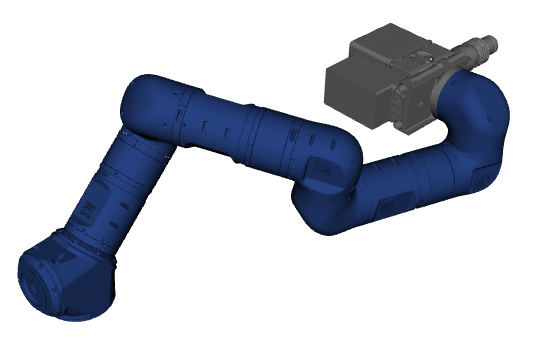
(a) C-1

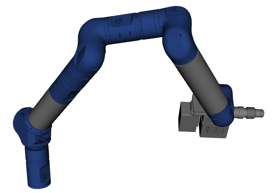
(b) C-2

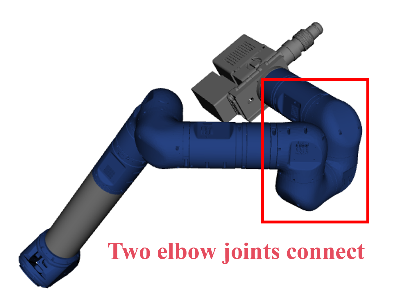
(c) C-3

Figure 5: The derived manipulator morphologies for the drilling task

V-E Experiments

We also conducted experiments with the CONCERT modular mobile manipulation robot executing the given drilling task to further validate the optimization results. The experiments snapshots can be obtained in Fig 6, from left to right in the images represent the morphology from C-1, C-2, and C-3, as illustrated in Fig. 5 For executing the task, the process begins with the assembly of the manipulator according to the desired morphology and adjusting it to the initial joint state. The initial joint state is also the warm-start of the MPC controller, which has record during the optimization as we introduced in the SEC. V-C’s third paragraph. Subsequently, MPC is applied as the controller for the modular manipulator with the given warm-start to track the reference trajectory in the task space. The experimental execution of the task, which considers different optimization objectives, can be found in the attached video. Notably, the mobile platform pose represents the initial pose corresponding to the desired mounted pose of the base link. At this juncture, the end-effector’s pose of the manipulator corresponds to the first desired point on the trajectory. During the execution of the task the effort of the robot joints remained within the maximum continues limits considered. It also shows that the robot avoids collisions with the mobile base of the robot and the wall in the environment.

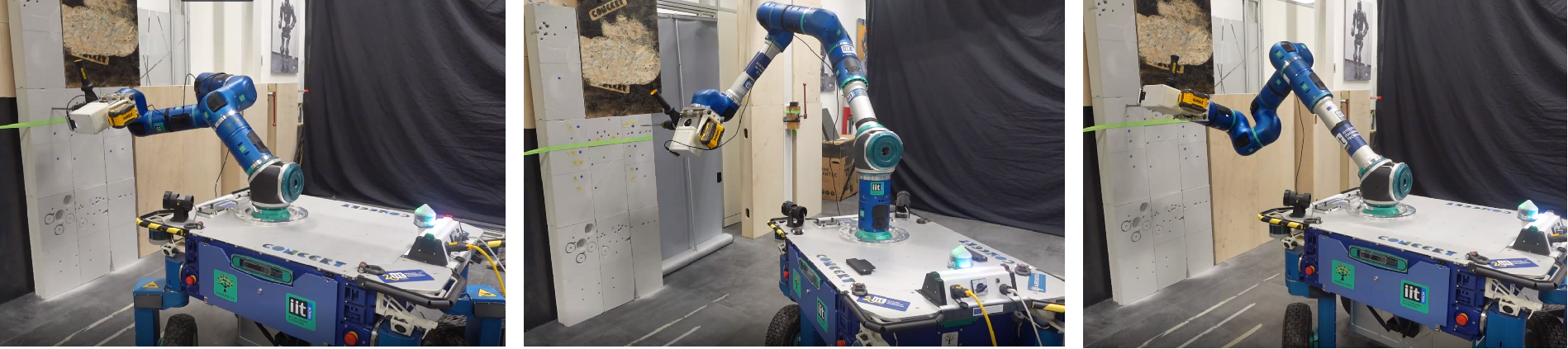
Figure 6: Snapshots of the experiments for various computational results.

VI Conclusion

This paper introduces a computational framework for simultaneously optimizing modular manipulators’ physical structure and mounted pose, ensuring their customization for specific tasks. Initially, we developed a mapping function that converts the discrete morphology state into a continuous modular state. This approach enables the implicit representation of the morphology state, allowing it to be optimized concurrently alongside the mounted pose of the manipulator within continuous space. Compared to our previous work, which tackled such issues through combinatorial optimization, this methodology accelerates the convergence speed and facilitates the attainment of more optimal solutions. Finally, we conducted experiments using the CONCERT modular mobile manipulation robot in practical scenarios, such as executing drilling tasks, a common application in construction environments.

References

- [1] E. Romiti, J. Malzahn, N. Kashiri, F. Iacobelli, M. Ruzzon, A. Laurenzi, E. M. Hoffman, L. Muratore, A. Margan, L. Baccelliere, et al., “Toward a plug-and-work reconfigurable cobot,” T-Mech, vol. 27, no. 5, pp. 3219–3231, 2021.
- [2] F. Cursi, W. Bai, E. M. Yeatman, and P. Kormushev, “Optimization of surgical robotic instrument mounting in a macro–micro manipulator setup for improving task execution,” T-RO, vol. 38, no. 5, pp. 2858–2874, 2022.
- [3] X. Qin, H. Zhang, T. Zhou, and Z. Xiong, “Where to install the manipulator: Optimal installation pose planning based on whale algorithm,” in 2022 AIM, pp. 962–967, IEEE, 2022.
- [4] W. K. Chung, J. Han, Y. Youm, and S. Kim, “Task based design of modular robot manipulator using efficient genetic algorithm,” in 1997 ICRA, vol. 1, pp. 507–512, IEEE, 1997.
- [5] E. Romiti, F. Iacobelli, M. Ruzzon, N. Kashiri, J. Malzahn, and N. Tsagarakis, “An optimization study on modular reconfigurable robots: Finding the task-optimal design,” in 2023 CASE, pp. 1–8, IEEE, 2023.
- [6] J. Külz and M. Althoff, “Optimizing modular robot composition: A lexicographic genetic algorithm approach,” arXiv preprint arXiv:2309.08399, 2023.
- [7] I.-M. Chen and G. Yang, “Automatic model generation for modular reconfigurable robot dynamics,” 1998.
- [8] A. Zhao, J. Xu, M. Konaković-Luković, J. Hughes, A. Spielberg, D. Rus, and W. Matusik, “Robogrammar: graph grammar for terrain-optimized robot design,” TOG, vol. 39, no. 6, pp. 1–16, 2020.
- [9] N. Hansen, S. D. Müller, and P. Koumoutsakos, “Reducing the time complexity of the derandomized evolution strategy with covariance matrix adaptation (cma-es),” Evolutionary computation, vol. 11, no. 1, pp. 1–18, 2003.
- [10] A. Radford, K. Narasimhan, T. Salimans, I. Sutskever, et al., “Improving language understanding by generative pre-training,” 2018.
- [11] R. Yu, K. Yang, and B. Guo, “The interaction graph auto-encoder network based on topology-aware for transferable recommendation,” in Proceedings of the 31st ACM International Conference on Information & Knowledge Management, pp. 2403–2412, 2022.
- [12] M. Lei, L. Lu, A. Laurenzi, L. Rossini, E. Romiti, J. Malzahn, and N. G. Tsagarakis, “An mpc-based framework for dynamic trajectory re-planning in uncertain environments,” in 2022 IEEE Humanoids, pp. 594–601, IEEE, 2022.
- [13] S. B. Liu and M. Althoff, “Optimizing performance in automation through modular robots,” in 2020 ICRA, pp. 4044–4050, IEEE, 2020.
- [14] E. Romiti, N. Kashiri, J. Malzahn, and N. Tsagarakis, “Minimum-effort task-based design optimization of modular reconfigurable robots,” in 2021 ICRA, pp. 9891–9897, IEEE, 2021.
- [15] A. Sathuluri, A. V. Sureshbabu, and M. Zimmermann, “Robust co-design of robots via cascaded optimisation,” in 2023 ICRA, pp. 11280–11286, IEEE, 2023.
- [16] S. Sivanandam, S. Deepa, S. Sivanandam, and S. Deepa, Genetic algorithms. Springer, 2008.
- [17] S. Ha, S. Coros, A. Alspach, J. M. Bern, J. Kim, and K. Yamane, “Computational design of robotic devices from high-level motion specifications,” T-RO, vol. 34, no. 5, pp. 1240–1251, 2018.
- [18] R. Koike, R. Ariizumi, and F. Matsuno, “Simultaneous optimization of discrete and continuous parameters defining a robot morphology and controller,” IEEE Transactions on Neural Networks and Learning Systems, 2023.
- [19] J. Hu, J. Whitman, and H. Choset, “Glso: Grammar-guided latent space optimization for sample-efficient robot design automation,” in CoRL, pp. 1321–1331, PMLR, 2023.
- [20] J. Pan, S. Chitta, and D. Manocha, “Fcl: A general purpose library for collision and proximity queries,” in 2012 ICRA, pp. 3859–3866, IEEE, 2012.