A Full Adagrad algorithm with $O(Nd)$ operations

Abstract

A novel approach is given to overcome the computational challenges of the full-matrix Adaptive Gradient algorithm (Full AdaGrad) in stochastic optimization. By developing a recursive method that estimates the inverse of the square root of the covariance of the gradient, alongside a streaming variant for parameter updates, the study offers efficient and practical algorithms for large-scale applications. This innovative strategy significantly reduces the complexity and resource demands typically associated with full-matrix methods, enabling more effective optimization processes. Moreover, the convergence rates of the proposed estimators and their asymptotic efficiency are given. Their effectiveness is demonstrated through numerical studies.

Keywords: Stochastic Optimization; Robbins-Monro algorithm; AdaGrad; Online estimation

1 Introduction

Stochastic optimization plays a crucial role in machine learning and data science, particularly relevant in the context of high-dimensional data (Genevay et al.,, 2016; Bottou et al.,, 2018; Sun et al.,, 2019). This paper focuses on the stochastic gradient-based methods. It targets on a scalar objective function $f(X,\theta)$, where $X$ is a random variable taking values in a measurable space $\mathcal{X}$ and $\theta$ is a parameter vector in $\mathbb{R}^{d}$. This function is assumed to be differentiable with respect to $\theta$. Our goal is to minimize the expected value of this function, denoted as $F(\theta):=\mathbb{E}\left[f(X,\theta)\right]$, in relation to $\theta$. The realizations of $X$ at different time steps are denoted as $X_{1},\cdots,X_{t},\cdots$, and $g_{t}(\theta):=\nabla_{\theta}f(X_{t},\theta)$ refers to the gradient of $f(X_{t},\cdot)$.

A popular approach in addressing this problem of optimization is Stochastic Gradient Descent(SGD), introduced by Robbins and Monro, (1951). It recursively updates the parameter estimate based on the last estimate of the gradient, i.e.

$$\theta_{t}=\theta_{t-1}-\nu_{t}g_{t}(\theta_{t-1}),$$

where $\nu_{t}$ is the learning rate and $\theta_{0}$ is arbitrarily chosen. Despite its computational efficiency and favorable convergence properties, SGD faces limitations, particularly in adapting the learning rate to the varying scales of features (Ruder,, 2016).

To address these limitations, many extensions of SGD have been proposed. A widely used variant is the Adaptive Gradient algorithm (AdaGrad) introduced by Duchi et al., (2011). It adapts the learning rate for each parameter, offering improved performances on problems with sparse gradients. The full-matrix version of AdaGrad can be expressed as follows:

$$\theta_{t}=\theta_{t-1}-\nu_{t}\mathcal{G}_{t}^{-1/2}g_{t}(\theta_{t-1}),$$

where $\mathcal{G}_{t}:=\sum^{t}_{k=1}g_{k}(\theta_{k-1})g_{k}(\theta_{k-1})^{T}$ is a recursive estimate of the covariance matrix of the gradient and $\mathcal{G}_{t}^{-1/2}$ is the inverse of the square root of it. However, a notable challenge with AdaGrad is computing the square root of the inverse of $\mathcal{G}_{t}$. This computation is particularly demanding in terms of computational resources, with a complexity of order $\mathcal{O}(d^{3})$. Such complexity is often prohibitive, especially in scenarios involving high-dimensional data. To deal with it, a diagonal version of AdaGrad was proposed, simplifying the process by using only the diagonal elements of $\mathcal{G}_{t}$, i.e

$$\theta_{t}=\theta_{t-1}-\nu_{t}\text{diag}\left(\mathcal{G}_{t}\right)^{-1/2}g_{t}(\theta_{t-1}).$$ (1)

In practice, this approach is more feasible and is broadly applied for machine learning tasks (Dean et al.,, 2012; Seide et al.,, 2014; Smith,, 2017). Furthermore, Défossez et al., (2022) establishes the standard convergence rate for Adagrad in the non convex case. Despite being more practical, the diagonal version of AdaGrad inherently loses information compared to the full-matrix version, especially in the case where the gradient have coordinates highly correlated.

Our work focuses on the full-matrix version of AdaGrad, proposing a recursive method to estimate the inverse of the square root of the covariance matrix $\Sigma:=\mathbb{E}\left[\nabla_{\theta}f(X,\theta^{*})\nabla_{\theta}f(X,\theta^{*})^{T}\right],$ where $\theta^{*}$ minimizes the function $F$. Unlike the original Full AdaGrad, which uses $G_{t}$ to estimate $\Sigma$ and then computes $G_{t}^{-1/2}$, we will directly estimate $\Sigma^{-1/2}$. Using the fact that

$$\Sigma^{-1/2}\Sigma\Sigma^{-1/2}-I_{d}=\mathbb{E}\left[\Sigma^{-1/2}\nabla_{\theta}f(X,\theta^{*})\nabla_{\theta}f(X,\theta^{*})^{T}\Sigma^{-1/2}-I_{d}\right]=0,$$

we introduce a Robbins-Monro algorithm to estimate $\Sigma^{-1/2}$. This estimator, denoted as $A_{t}$, is defined recursively for all $t\geq 1$, by:

$$A_{t}=A_{t-1}-\gamma_{t}\left(A_{t-1}g_{t}(\theta_{t-1})g_{t}(\theta_{t-1})^{T}A_{t-1}-I_{d}\right),$$

where $A_{0}=I_{d}$ and $(\gamma_{t})_{t\geq 1}$ is a sequence of positive real numbers, decreasing towards 0. This estimate is used in updating the estimate of $\theta$:

$$\theta_{t}=\theta_{t-1}-\nu_{t}A_{t-1}g_{t}(\theta_{t-1}).$$

Consequently, this approach enables us to avoid the expensive computation of the square root of the inverse of $\mathcal{G}_{t}$, enhancing the computational efficiency of the algorithm. Nevertheless, $A_{t}$ is not necessarily positive definite, and we so propose a slight modification in this sense. In addition, $\theta_{t}$ cannot be asymptotically efficient, and we so introduced its (weighted) averaged version (Polyak and Juditsky,, 1992; Pelletier,, 2000; Mokkadem and Pelletier,, 2011; Boyer and Godichon-Baggioni,, 2023).

Although the propose approach to estimate $\Sigma^{-1/2}$ enables to reduce the calculus time, this only enables to achieve a total complexity of order $O(Nd^{2})$, where $N$ is the sample size. Then, we propose a Streaming version of our algorithm, updating the estimate of $\Sigma^{-1/2}$ and $\theta$ only after observing every $n$ gradients and using their average. This approach further reduces the algorithm’s complexity, making it more practical for large-scale applications. More precisely, a good choice of $n$ ($n=d$ for instance) enables to obtain asymptotically efficient estimates with a complexity of order $O(Nd)$, i.e. with the same complexity as for Adagrad algorithm.

The paper is organized as follows. The general framework is introduced in Section 2. In Section 3, we present a detailed description of the proposed Averaged Full AdaGrad algorithm before establishing its asymptotic efficiency. Following this, we introduce a streaming variant of the Full AdaGrad algorithm in 4 and we obtain the asymptotic efficiency of the proposed estimates. In Section 5, we illustrate the practical applicability of our algorithms through numerical studies. The proofs are postponed in Section 6.

2 Framework

Let us recall that the aim is to minimize the functional $F:\mathbb{R}^{d}\longrightarrow\mathbb{R}$ defined for all $\theta\in\mathbb{R}^{d}$ by:

$$F(\theta):=\mathbb{E}\left[f(X,\theta)\right],$$

where $f:\mathcal{X}\times\mathbb{R}^{d}\to\mathbb{R}$. In all the sequel, we suppose that the following assumptions are fulfilled:

Assumption 1

The function $F$ is strictly convex, twice continuously differentiable, and there is $\theta^{*}\in\mathbb{R}^{d}$ such that $\nabla F(\theta^{*})=0$.

This assumption ensures that $\theta^{*}$ is the unique minimizer of the functional $F$ and legitimates the use of gradient-type methods.

Assumption 2

There exists an integer $p\geq 1$ and a positive constant $C_{p}<\infty$ such that for all $\theta\in\mathbb{R}^{d}$

$$\mathbb{E}\left[\left\|\nabla_{\theta}f(X,\theta)\right\|^{2p}\right]\leq C_{p}+C_{p}\left(F(\theta)-F(\theta^{*})\right)^{p}.$$

In the literature on stochastic gradient algorithms, it is common to consider moments of order 2 ($p=1$) or 4 ($p=2$) for the gradient of $f$ (see, e.g., Pelletier, (1998, 2000)). However, due to some hyperparameters within our algorithm, we must strongly constraint the moment order of the gradient of $f$ when determining the convergence rate of our estimates. The specific value of $p$ will be delineated in the theorem statements.

Assumption 3

The function $\Sigma:\theta\longmapsto\mathbb{E}\left[\nabla_{\theta}f(X,\theta)\nabla_{\theta}f(X,\theta)^{T}\right]$ is $L_{\Sigma}$-Lipschitz and $\Sigma\left(\theta^{*}\right)$ is positive.

This assumption is quite specific to our work on FullAdagrad as it ensures the convergence of estimates of the variance, and more specifically in our case, of the square root of their inverse. It is worth noting that this assumption is quite common in the literature, particularly when considering the estimation of asymptotic covariance (Zhu et al.,, 2023; Godichon-Baggioni and Lu,, 2024).

The above are assumptions regarding the first-order derivatives of $F$. Next, we present some necessary assumptions concerning the second-order derivatives of the function.

Assumption 4

The Hessian of $F$ is uniformly bounded by $L_{\nabla F}$.

This assumption ensures that the gradient of $F$ is $L_{\nabla F}$-Lipschitz which is crucial to obtain the consistency of the estimates (via a Taylor’s expansion of the gradient at order $2$).

Assumption 5

The Hessian of $F$ is Locally Lipschitz: there exists $\eta>0$ and $L_{\eta}>0$ such that for all $\theta\in\mathcal{B}\left(\theta^{*},\eta\right)$,

$$\left\|\nabla F(\theta)-\nabla^{2}F\left(\theta^{*}\right)\left(\theta-\theta^{*}\right)\right\|\leq L_{\eta}\left\|\theta-\theta^{*}\right\|^{2}.$$

These assumptions are close to those found in the literature (Pelletier,, 2000; Gadat and Panloup,, 2023; Boyer and Godichon-Baggioni,, 2023). The main differences come from Assumption 2 and 3. These last ones are crucial for the theoretical study of the estimates of $\Sigma^{-1/2}$, i.e. to prove their strong consistency.

3 A Full AdaGrad algorithm with $\mathcal{O}(td^{2})$ operations

In this section, we introduce a Full AdaGrad algorithm with $\mathcal{O}(td^{2})$ operations. We focus on recursively estimating $\Sigma^{-1/2}$ using a Robbins-Monro algorithm, in order to refine estimates of $\theta^{*}$ while ensuring computational performance.

3.1 Estimating $\Sigma^{-1/2}$ with the help of a Robbins-Monro algorithm

First, we focus on recursive estimates of the matrix $\Sigma^{-1/2}$. In all the sequel, let $X_{1},\ldots,X_{t},\ldots$ be i.i.d. copies of $X$ and for all $\theta\in\mathbb{R}^{d}$, we denote $g_{t}(\theta):=\nabla_{\theta}f(X_{t},\theta)$. Let us recall that the Robbins-Monro algorithm for estimating $\Sigma^{-1/2}$, described in the Introduction, is defined recursively for all $t\geq 0$ by

$$A_{t+1}=A_{t}-\gamma_{t+1}\left(A_{t}g_{t+1}(\theta_{t})g_{t+1}(\theta_{t})^{T}A_{t}-I_{d}\right),$$

where $A_{0}$ is a symmetric positive definite matrix, $(\theta_{t})_{t\geq 0}$ is a sequence of estimates of $\theta^{*}$, and $\gamma_{t}=c_{\gamma}t^{-\gamma}$ with $c_{\gamma}>0$ and $1/2<\gamma<1$. Observe that $A_{t+1}g_{t}(\theta_{t})$ is a vector, implying that the complexity of this operation is of order $O(d^{2})$. However, we cannot ensure that the matrix $A_{t}$ is always positive definite. Nevertheless, in Full AdaGrad, $A_{t}$ must always be positive to guarantee that at each step, we go in the direction of the gradient (in average). To address this issue, we propose a slightly modified version of $A_{t}$ by defined for all $t\geq 0$ by

$$A_{t+1}=A_{t}-\gamma_{t+1}\left(A_{t}g_{t+1}\left(\theta_{t}\right)g_{t+1}\left(\theta_{t}\right)^{T}A_{t}-Id\right)\mathbf{1}_{\left\{g_{t+1}\left(\theta_{t}\right)^{T}A_{t}g_{t+1}\left(\theta_{t}\right)\leq\beta_{t+1}\right\}},$$

where $\beta_{t}=c_{\beta}t^{\beta}$ with $0<\beta<1/2$ and $0<c_{\beta}c_{\gamma}<1$. In fact, $g_{t+1}(\theta_{t})^{T}A_{t}g_{t+1}(\theta_{t})$ is the unique positive eigenvalue of the rank-1 matrix $A_{t}g_{t+1}(\theta_{t})g_{t+1}(\theta_{t})^{T}$. We update $A_{t}$ only when this value is not excessively large and thanks to this modification, $A_{t}$ is positive definite for any $t\geq 0$.

3.2 Full AdaGrad algorithms with $\mathcal{O}(td^{2})$ operations

We can now propose a Full AdaGrad algorithm defined for all $t\geq 0$ by

$$\theta_{t+1} =\theta_{t}-\nu_{t+1}A_{t}g_{t+1}\left(\theta_{t}\right),$$ (2)

$$A_{t+1} =A_{t}-\gamma_{t+1}\left(A_{t}g_{t+1}\left(\theta_{t}\right)g_{t+1}\left(\theta_{t}\right)^{T}A_{t}-Id\right)\mathbf{1}_{\left\{g_{t+1}\left(\theta_{t}\right)^{T}A_{t}g_{t+1}\left(\theta_{t}\right)\leq\beta_{t+1}\right\}},$$ (3)

where $\theta_{0}$ is arbitrarily chosen. Although our numerical studies show that this algorithm performs well (see Section 5), the obtained estimates are not asymptotically efficient. Therefore, to ensure the asymptotic optimality of the estimates, and to enhance the performance of the algorithm in practice, we follow the idea of Mokkadem and Pelletier, (2011); Boyer and Godichon-Baggioni, (2023). More precisely, we introduce the Weighted Averaged Full AdaGrad (WAFA for short) defined recursively for all $t\geq 0$ by

$$\theta_{t+1} =\theta_{t}-\nu_{t+1}A_{t}g_{t+1}\left(\theta_{t}\right)$$ (4)

$$\theta_{t+1,\tau} =\left(1-\frac{\ln(t+1)^{\tau}}{\sum_{k=0}^{t}\ln(k+1)^{\tau}}\right)\theta_{t,\tau}+\frac{\ln(t+1)^{\tau}}{\sum_{k=0}^{t}\ln(k+1)^{\tau}}\theta_{t+1}$$ (5)

$$A_{t+1} =A_{t}-\gamma_{t+1}\left(A_{t}g_{t+1}\left(\theta_{t,\tau}\right)g_{t+1}\left(\theta_{t,\tau}\right)^{T}A_{t}-Id\right)\mathbf{1}_{\left\{g_{t+1}\left(\theta_{t,\tau}\right)^{T}A_{t}g_{t+1}\left(\theta_{t,\tau}\right)\leq\beta_{t+1}\right\}}$$ (6)

$$A_{t+1,\tau^{\prime}} =\left(1-\frac{\ln(t+1)^{\tau^{\prime}}}{\sum_{k=0}^{t}\ln(k+1)^{\tau^{\prime}}}\right)A_{t,\tau^{\prime}}+\frac{\ln(t+1)^{\tau^{\prime}}}{\sum_{k=0}^{t}\ln(k+1)^{\tau^{\prime}}}A_{t+1}$$ (7)

with $\theta_{0,\tau}=\theta_{0}$, $A_{0,\tau^{\prime}}=A_{0}$ and $\tau,\tau^{\prime}\geq 0$. Note that when $\tau,\tau^{\prime}=0$, we obtain the usual averaged estimates. However, taking both greater than zero allows to place more weight on the recent estimations, which are supposed to be better. The following theorem gives the strong consistency of the Full Adagrad estimates of $\theta^{*}$.

Theorem 3.1

Suppose Assumptions 1, 2 and 4 hold. Suppose also that $2\gamma+2\nu>3$ and $\nu+\beta<1$. Then $\theta_{t}$ and $\theta_{t,\tau}$ defined by (4) and (5) converge almost surely to $\theta^{*}$.

The proof is given in Section 6. The hyperparameters constraints introduced here are for technical reasons. These conditions are not necessary in practice (see Section 5). In the following theorem, we establish the strong consistency of the estimates of $\Sigma^{-1}$ and the almost sure convergence rates of the estimates of $\theta^{*}$.

Theorem 3.2

Suppose Assumptions 1, 3 and 4 hold as well as 2 with $p>\max\left\{\frac{8-8\gamma}{\gamma+\beta-1},2\left(\frac{1}{\gamma}-1\right)\right\}$. Suppose also that $2\gamma+2\nu>3$, $\nu+\beta<1$, $2\gamma-2\beta>1$ and that $\gamma+\beta>1$. Then

$$A_{t}\xrightarrow[t\to+\infty]{a.s}\Sigma^{-1/2}\quad\quad\text{ and }\quad\quad A_{t,\tau^{\prime}}\xrightarrow[t\to+\infty]{a.s}\Sigma^{-1/2}$$

In addition,

$$\left\|\theta_{t}-\theta^{*}\right\|^{2}=O\left(\frac{\ln t}{t^{\nu}}\right)\quad a.s.\quad\quad\text{ and }\quad\quad\left\|\theta_{t,\tau}-\theta^{*}\right\|^{2}=O\left(\frac{\ln t}{t^{\nu}}\right)\quad a.s.$$

The proof is given in Section 6. Observe that the conditions on $\gamma,\nu,\beta$ imply that $\nu<\gamma$ and $\gamma>3/4$. These conditions are due to the use of Robbins-Siegmund Theorem and should be certainly improved. Indeed, we will see in Section 5 that these conditions do not need to be fulfilled in practice. Finally, under slightly restricted conditions, the following theorem gives better convergence rates of $\theta^{*}$.

Theorem 3.3

Suppose Assumptions 1, 3, 4 and 5 hold as well as 2 with $p>\max\left\{\frac{8-8\gamma}{\gamma+\beta-1},2\left(\frac{1}{\gamma}-1\right)\right\}$. Suppose also that $2\gamma+2\nu>3$, $\nu+\beta<1$, $2\gamma-2\beta>1$ and that $\gamma+\beta>1$. Then,

$$\left\|\theta_{t,\tau}-\theta^{*}\right\|^{2}=O\left(\frac{\ln t}{t}\right)\quad a.s.\quad\quad\text{ and }\quad\quad\sqrt{t}\left(\theta_{t,\tau}-\theta^{*}\right)\xrightarrow[t\to+\infty]{\mathcal{L}}\mathcal{N}\left(0,H^{-1}\Sigma H^{-1}\right)$$

with $\Sigma:=\Sigma(\theta^{*})$ and $H:=\nabla^{2}F(\theta^{*})$.

The proof is given in Section 6. Thus, we obtain the asymptotic efficiency of the weighted averaged estimate. In addition, these last ones only necessitates $O(Nd^{2})$ operations, compare it a complexity of order $O(Nd^{3})$ operations if we directly calculate $\mathcal{G}_{t}^{-1/2}$.

4 A Streaming Full AdaGrad algorithm with $\mathcal{O}(N_{t}d)$ operations

In this section,, following the idea of Godichon-Baggioni and Werge, (2023), we introduce a Streaming Weighted Averaged Full AdaGrad algorithm (SWAFA for short) to reduce the computational complexity of the algorithm. We consider that samples arrive (or are dealt with) by blocks of size $n\in\mathbb{N}$. More precisely, we suppose that at time $t$, we have $n$ new i.i.d copies of $X$ denoted as $(X_{t,1},\ldots,X_{t,n})$. Therefore, at time $t$, we will have observed a total of $N_{t}=nt$ i.i.d copies of $X$.

In this scenario, let us denote $g_{t+1}(\theta_{t})=\frac{1}{n}\sum_{i=1}^{n}\nabla_{\theta}f(X_{t+1,i},\theta_{t})$. Then, the streaming algorithm is defined recursively for all $t\geq 0$ by

$$\theta_{t+1} =\theta_{t}-\nu_{t+1}A_{t}g_{t+1}\left(\theta_{t}\right)$$ (8)

$$\theta_{t+1,\tau} =\left(1-\frac{\ln(t+1)^{\tau}}{\sum_{k=0}^{t}\ln(k+1)^{\tau}}\right)\theta_{t,\tau}+\frac{\ln(t+1)^{\tau}}{\sum_{k=0}^{t}\ln(k+1)^{\tau}}\theta_{t+1}$$ (9)

$$A_{t+1} =A_{t}-\gamma_{t+1}\left(nA_{t}g_{t+1}\left(\theta_{t,\tau}\right)g_{t+1}\left(\theta_{t,\tau}\right)^{T}A_{t}-Id\right)\mathbf{1}_{\left\{ng_{t+1}\left(\theta_{t,\tau}\right)^{T}A_{t}g_{t+1}\left(\theta_{t,\tau}\right)\leq\beta_{t+1}\right\}}$$ (10)

$$A_{t+1,\tau^{\prime}} =\left(1-\frac{\ln(t+1)^{\tau^{\prime}}}{\sum_{k=0}^{t}\ln(k+1)^{\tau^{\prime}}}\right)A_{t,\tau^{\prime}}+\frac{\ln(t+1)^{\tau^{\prime}}}{\sum_{k=0}^{t}\ln(k+1)^{\tau^{\prime}}}A_{t+1}$$ (11)

Then, we still have $O(d^{2})$ operations for updating $A_{t},A_{t,\tau^{\prime}}$ and $\theta_{t}$. Nevertheless, we only have $t=\frac{N_{t}}{n}$ iterations. This leads to total number of operations of order $O(N_{t}d^{2}n^{-1})$ operations detailed as follows:

$$\underbrace{N_{t}d+\frac{N_{t}d^{2}}{n}}_{\text{updating }\theta_{t},A_{t},A_{t,\tau^{\prime}}}+\underbrace{\frac{N_{t}d}{n}}_{\text{updating }\theta_{t,\tau}}.$$

Considering $n=d$ enables the complexity of the algorithm to be reduced to $\mathcal{O}(N_{t}d)$ operations, which is equivalent to the complexity of the AdaGrad algorithm defined by (1). We next give three theorems that establish the strong consistency, convergence rates, and asymptotic efficiency of the SWAFA estimates.

Theorem 4.1

Suppose Assumptions 1 and 4 hold. Suppose also that $2\gamma+2\nu>3$ and $\nu+\beta<1$. Then $\theta_{t}$ and $\theta_{t,\tau}$ defined by (8) and (9) converge almost surely to $\theta^{*}$.

The proof is very similar to the one of Theorem 3.1 and is therefore not given.

Theorem 4.2

Suppose Assumptions 1, 3 and 4 hold as well as 2 with $p>\max\left\{\frac{8-8\gamma}{\gamma+\beta-1},2\right\}$. Suppose also that $2\gamma+2\nu>3$, $\nu+\beta<1$, $2\gamma-2\beta>1$, $6\gamma+2\nu>7$ and that $\gamma+\beta>1$. Then

$$A_{t}\xrightarrow[t\to+\infty]{a.s}\Sigma^{-1/2}\quad\quad\text{ and }\quad\quad A_{t,\tau^{\prime}}\xrightarrow[t\to+\infty]{a.s}\Sigma^{-1/2}$$

In addition, $\theta_{t}$ and $\theta_{t,\tau}$ defined by (8) and (9) satisfy

$$\left\|\theta_{t}-\theta^{*}\right\|^{2}=O\left(\frac{\ln t}{t^{\nu}}\right)\quad a.s.\quad\quad\text{ and }\quad\quad\left\|\theta_{t,\tau}-\theta^{*}\right\|^{2}=O\left(\frac{\ln t}{t^{\nu}}\right)\quad a.s.$$

The proof is given in Section 6. Again, the restricted conditions on $\gamma,\nu,\beta$ are due to the use of Robbins-Siegmund Theorem and should be improved.

Theorem 4.3

Suppose Assumptions 1, 3, 4 and 5 hold as well as 2 for $p>\max\left\{\frac{8-8\gamma}{\gamma+\beta-1},2\right\}$. Suppose also that $2\gamma+2\nu>3$, $\nu+\beta<1$, $2\gamma-2\beta>1$, $6\gamma+2\nu>7$ and that $\gamma+\beta>1$. Then $\theta_{t,\tau}$ defined by (9) satisfy

$$\left\|\theta_{t,\tau}-\theta^{*}\right\|^{2}=O\left(\frac{\ln nt}{nt}\right)\quad a.s.\quad\quad\text{ and }\quad\quad\sqrt{nt}\left(\theta_{t,\tau}-\theta^{*}\right)\xrightarrow[t\to+\infty]{\mathcal{L}}\mathcal{N}\left(0,H^{-1}\Sigma H^{-1}\right)$$

with $\Sigma:=\Sigma\left(\theta^{*}\right)$ and $H:=\nabla^{2}F\left(\theta^{*}\right)$.

The proof is very similar to the one of Theorem 3.3 and is therefore not given. Note that we ultimately obtain $\|\theta_{t,\tau}-\theta^{*}\|^{2}=O\left(\frac{\ln N_{t}}{N_{t}}\right)$ a.s., which means the convergence rate is the same as the one of the WAFA algorithm and the estimates are still asymptotically efficient, but we drastically reduce the calculus time.

5 Applications

In this section, we carry out some numerical experiments to investigate the performance of our proposed Full AdaGrad and Streaming Full AdaGrad algorithms. Our investigation begins with the application of these algorithms to the linear regression model on simulated data. The choice of linear regression is strategic. Indeed, with this model we are able to obtain the exact values of the matrix $\Sigma=\Sigma(\theta^{*})$, which allows us to also evaluate the performances of our estimates of $\Sigma^{-1/2}$. Furthermore, we extend our experimentation to real-world data by applying our algorithms to logistic regression tasks. It tests the adaptability of our proposed methods in handling complex, real-life datasets. Throughout these comparative experiments, we employ the AgaGrad algorithm defined in (1) and its weighted averaged version as a benchmark. The Weighted Averaged AdaGrad (WAA) is formulated following the same principles as those outlined for $\theta_{t,\tau}$ in (5).

5.1 Discussion about the hyper-parameters involved in the different algorithms

Although in the previous sections, we imposed several restrictions on hyperparameters $\beta$, $\gamma$, and $\nu$ purely for technical reasons to derive the convergence rates of the algorithms theoretically, in our experiments, we simply set $\beta=\gamma=\nu=\frac{3}{4}$. We will demonstrate that such a choice of hyperparameters does not affect the practical performance of the algorithms. Furthermore, for Full AdaGrad, we choose $c_{\beta}=c_{\gamma}=c_{\nu}=1$, but for Full AdaGrad Streaming, while $c_{\beta}$ and $c_{\gamma}$ are still set to 1, we set $c_{\nu}=\sqrt{n}$. Since Full AdaGrad Streaming updates $\theta_{t}$ only $\frac{1}{n}$ times as often as Full AdaGrad and AdaGrad , we increase the step size of each $\theta_{t}$ update in Full AdaGrad Streaming by choosing a larger $c_{\nu}$. However, for the AdaGrad algorithm defined in (1), we set $\nu_{t}=t^{-1/4}$, since $\left\{\mathcal{G}_{t}\right\}^{-1/2}$ inherently converges to zero at a rate of $1/\sqrt{t}$. For the Full AdaGrad algorithms, we always initialize $A_{0}$ as $0.1I_{d}$. Finally, we set $\tau,\tau^{\prime}=2$ for all weighted averaged estimates.

5.2 Linear regression on simulated data

We first perform experiments with simulated data, considering the linear regression model. Let $(X,Y)$ be a random vector taking values in $\mathbb{R}^{d}\times\mathbb{R}$. Consider the case where $X$ is a centered Gaussian random vector and

$$Y=X^{T}\theta^{*}+\varepsilon,$$

where $\theta^{*}$ is a parameter of $\mathbb{R}^{d}$ and $\varepsilon\sim\mathcal{N}(0,1)$ is independent from $X$. If the matrix $\mathbb{E}[XX^{T}]$ is positive, $\theta^{*}$ is the unique minimizer of the function $F$ defined for all $h\in\mathbb{R}^{p}$ by

$$F(h)=\frac{1}{2}\mathbb{E}\left[(Y-h^{T}X)^{2}\right].$$

In the upcoming simulations, we fix $d=20$. For each sample, we simulate $N=30,000$ i.i.d copies of $X\sim\mathcal{N}(0,\Sigma_{X})$, where $\Sigma_{X}$ is a positive definite covariance matrix given later. Note that in this case the variance of the gradient satisfy $\Sigma=\Sigma_{X}$. Parameter $\theta^{*}$ is randomly selected as a realization from a uniform distribution over the hypercube $[-2,2]^{d}$. We then estimate $\theta^{*}$ using the different algorithms and compare their performances.

5.2.1 AdaGrad vs. Full AdaGrad

We first compare the performance of Full AdaGrad, AdaGrad and their weighted averaged versions. We consider two different structures for $\Sigma_{X}$. The first one is $\Sigma_{X}=I_{d}$, leading to the case of independent predictors. The second one is $\Sigma_{X}=R$ with $R_{i,j}=0.9^{\left|i-j\right|}$, leading to strong correlation between predictors. To compare the two algorithms, we compute the mean-squared error of the distance from $\theta_{t}$ to $\theta^{*}$ by averaging over 100 samples. We initialize $\theta_{0}$ as $\theta_{0}=\theta^{*}+\frac{1}{2}E$, where $E\sim\mathcal{N}(0,I_{d})$ for both algorithms. Figure 1 shows the evolution of the mean squared error with respect to the sample size for the four algorithms.

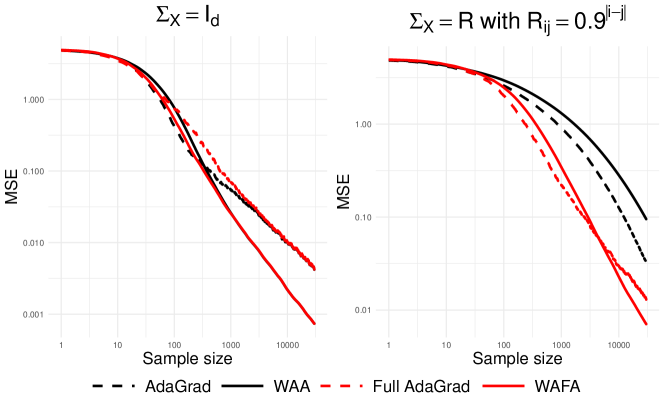
Figure 1: Linear regression case with $(N,d)=(30000,20)$. Mean squared error with respect to the sample size for AdaGrad and Full AdaGrad algorithms with their weighted averaged versions. Two values of $\Sigma_{X}$ are considered: $\Sigma_{X}=I_{d}$ (one the left) and $\Sigma_{X}=R$ (on the right).

When $\Sigma_{X}$ is the identity matrix, AdaGrad and FullAdaGrad perform almost identically, and without surprise, the weighted averaged estimates enables to accelerate the convergence. In this case, $\Sigma$ is a diagonal matrix, hence when AdaGrad only uses the diagonal elements, it does not lose any information. However, when there are strong correlations between predictors, as the off-diagonal elements of $\Sigma$ are no longer zero, Full AdaGrad significantly outperforms AdaGrad. This highlights the significance of using Full AdaGrad over AdaGrad when addressing non-diagonal variance.

5.2.2 Study of the full Adagrad streaming version.

In this section, we demonstrate that the SWAFA can run in shorter time on the same dataset compared to WAFA, while achieving comparable results. We consider three different block sizes: $n=d=20$, $n=5$, and $n=1$. Note that in the case $n=1$, SWAFA and WAFA algorithms are the same. We simulate the data in exactly the same manner as in the previous paragraph. Through 100 samples, we plot the algorithm’s running time, and the estimation error of $\theta$ given by $\left\|\theta_{t,\tau}-\theta^{*}\right\|$ for the three different block sizes. Moreover, since we have the exact values of $\Sigma$, we also evaluate the estimates of $\Sigma^{-1/2}$ by computing the error defined by $\left\|A_{t,\tau}-\Sigma^{-1/2}\right\|_{F}$.

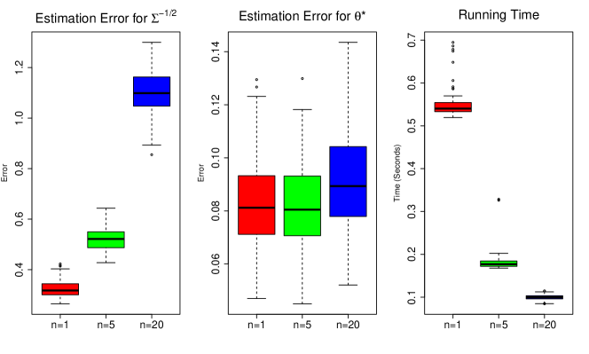
Figure 2: From the left to the right: boxplots of the estimation errors for $\Sigma^{-1/2}$, boxplot of the estimation errors for $\theta$ and boxplots of running time. In each case, $\Sigma_{X}=R$, $(N,d)=(30000,20)$ and three possible values of the streaming batch size are considered: $n=1,5,20$.

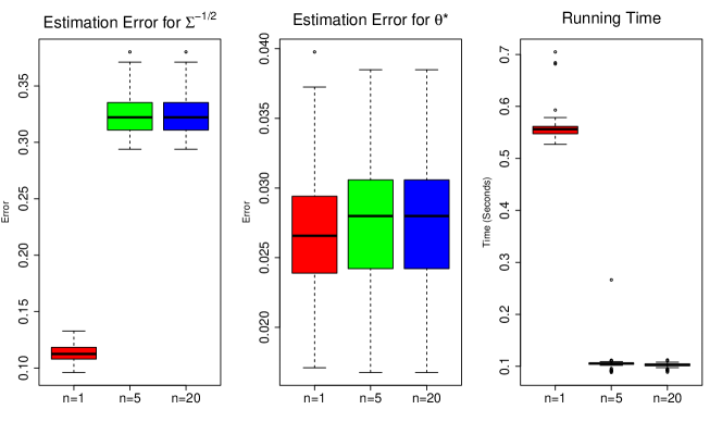
Figure 3: From the left to the right: boxplots of the estimation errors for $\Sigma^{-1/2}$, boxplot of the estimation errors for $\theta$ and boxplots of running time. In each case, $\Sigma_{X}=I_{d}$, $(N,d)=(30000,20)$ and three possible values of the streaming batch size are considered: $n=1,5,20$.

We can see from Figures 2 and 3 that SWAFA significantly reduced computation time. In fact, when $n=d=20$, the majority of computation time is spent on reading the data and estimating the gradient. SWAFA has a larger estimation error for $\Sigma^{-1/2}$ compared to WAFA, which is acceptable in practice, because it can still accurately estimate $\theta^{*}$.

Considering higher dimensions, we conducted the same experiments and obtained similar results which are given in the Appendix.

5.3 Logistic regression on real data

Now, we apply algorithms to real-world data. We use the COVTYPE dataset, which was initially collected by Blackard, (1998). This dataset contains information on 581,011 areas and 54 different features and is often used in research (Lazarevic and Obradovic,, 2002; Toulis and Airoldi,, 2017; Reagen et al.,, 2016). Our focus is on the most common forest cover type, ”Spruce/Fir,” accounting for about half of the data set. We have simplified the ”covertype” variable for our analysis by marking ”Spruce/Fir” as 1 and all other types as 0. The objective is to use logistic regression to predict this binary variable. The data is split into two portions: 50% for training and 50% for testing. We apply AdaGrad, Full AdaGrad, WAA, WAFA, and SWAFA with $n=d=54$. We calculate their accuracy on both the training and testing sets. For all algorithms, we initialize $\theta_{0}=(0,\ldots,0)$.

	Full AdaGrad	WAFA	SWAFA	AdaGrad	WAA
Training Accuracy(%)	75.67	75.58	75.59	75.71	75.56
Test Accuracy(%)	75.69	75.61	75.62	75.74	75.58

Table 1: Accuracy of AdaGrad, Full AdaGrad, WAA, WAFA, and SWAFA on ”COVTYPE” dataset.

Since this experiment is based on real data, the real parameter $\theta^{*}$ remains unknown to us, making it impossible to determine the accuracy of the estimations. However, all five algorithms achieved almost identical correct classification rates, indicating that the proposed methods are applicable to real data.

Conclusion

This work propose novel approaches to Full AdaGrad algorithms. The core innovation lies in applying a Robbins-Monro type algorithm for estimating the inverse square root of the variance of the gradient. By proving the convergence rate of the proposed estimates, we lay a theoretical foundation that establishes the reliability of our approach. Through numerical studies, we have shown that our approach offers substantial advantages over traditional AdaGrad algorithms that rely solely on diagonal elements. Moreover, we introduce a streaming variant of our method, which further reduces computational complexity. We show that the streaming estimates are also asymptotically efficient. An extension of this work would be to understand the possible impact of the dimension of the behavior of the estimates, maybe through a non asymptotic theoretical study.

6 Proofs

To simplify our notation, in the following we denote $\widehat{\Sigma}_{t}=g_{t}(\theta_{t-1,\tau})g_{t}(\theta_{t-1,\tau})^{T}$ , $W_{t}:=g_{t+1}\left(\theta_{t,\tau}\right)g_{t+1}\left(\theta_{t,\tau}\right)^{T}A_{t}$ and $Q_{t}=A_{t}^{1/2}\widehat{\Sigma}_{t+1}A_{t}^{1/2}$ with $\left\|Q_{t}\right\|_{F}=g_{t+1}\left(\theta_{t,\tau}\right)^{T}A_{t}g_{t+1}\left(\theta_{t,\tau}\right)$.

6.1 Proof of Theorem 3.1

The aim is to apply Theorem 1 in Godichon-Baggioni and Werge, (2023). Observe that in the proof of this theorem, no assumption on the continuity of the function $\Sigma$ is used. Then, we just have to control the eigenvalues of the random stepsequence $A_{t,\tau^{\prime}}$. In this aim, we first give an upper bound of $\lambda_{\max}(A_{t})$ without requiring knowledge on the behavior of the estimate $\theta_{t}$.

Study on the largest eigenvalue of $A_{t}$ and $A_{t,\tau^{\prime}}$.

It is obvious that the matrix $A_{t}\widehat{\Sigma}_{t+1}A_{t}$ is positive semi-definite, so that

$$\lambda_{\max}(A_{t+1})\leq\lambda_{\max}\left(A_{t}+\gamma_{t+1}I_{d}\mathbf{1}_{\left\{\left\|Q_{t}\right\|_{F}\leq\beta_{t+1}\right\}}\right)\leq\lambda_{\max}\left(A_{t}+\gamma_{t+1}I_{d}\right)$$

Therefore,

$$\lambda_{\max}(A_{t+1})\leq\lambda_{\max}\left(A_{0}\right)+\sum_{k=0}^{t}\gamma_{k+1}=\mathcal{O}\left(t^{1-\gamma}\right),$$ (12)

and one can derive that $\lambda_{\max}\left(A_{t,\tau}\right)=O\left(t^{1-\gamma}\right)$ a.s.

Study on the smallest eigenvalue of $A_{t}$ and $A_{t,\tau^{\prime}}$.

We now provide an asymptotic bound of $\lambda_{\min}(A_{t})^{-1}$, without necessitating knowledge on the behavior of the estimate $\theta_{t}$. Thanks to the truncation term ($\mathbf{1}_{\left\|Q_{t}\right\|_{F}\leq\beta_{t+1}}$), one can easily verify that $A_{t}$ is positive for all $t\geq 0$. We now give a better lower bound of its eigenvalues. First, remark that since $A_{t}$ is symmetric and positive, one can rewrite $A_{t+1}$ as

$$A_{t+1} =A_{t}-\gamma_{t+1}A_{t}\widehat{\Sigma}_{t+1}A_{t}\mathbf{1}_{\left\{\left\|Q_{t}\right\|_{F}\leq\beta_{t+1}\right\}}+\gamma_{t+1}I_{d}\mathbf{1}_{\left\{\left\|Q_{t}\right\|_{F}\leq\beta_{t+1}\right\}}$$

$$=A_{t}^{1/2}\left(I_{d}-\gamma_{t+1}A_{t}^{1/2}\widehat{\Sigma}_{t+1}A_{t}^{1/2}\mathbf{1}_{\left\{\left\|Q_{t}\right\|_{F}\leq\beta_{t+1}\right\}}\right)A_{t}^{1/2}+\gamma_{t+1}I_{d}\mathbf{1}_{\left\{\left\|Q_{t}\right\|_{F}\leq\beta_{t+1}\right\}}$$ (13)

Note that by definition of $\widehat{\Sigma}_{t+1}$, the matrix $A_{t}^{1/2}\widehat{\Sigma}_{t+1}A_{t}^{1/2}$ is of rank $1$ and

$$\left\|A_{t}^{1/2}\widehat{\Sigma}_{t+1}A_{t}^{1/2}\right\|_{op}=\left\|A_{t}^{1/2}\widehat{\Sigma}_{t+1}A_{t}^{1/2}\right\|_{F}=\left\|Q_{t}\right\|_{F}.$$

Thus,

$$\lambda_{\min}(A_{t+1}) \geq\lambda_{\min}\left(A_{t}^{1/2}\left(I_{d}-\gamma_{t+1}A_{t}^{1/2}\widehat{\Sigma}_{t+1}A_{t}^{1/2}\mathbf{1}_{\left\{\left\|Q_{t}\right\|_{F}\leq\beta_{t+1}\right\}}\right)A_{t}^{1/2}\right)+\gamma_{t+1}\mathbf{1}_{\left\{\left\|Q_{t}\right\|_{F}\leq\beta_{t+1}\right\}}$$

$$\geq\lambda_{\min}(A_{t})\left(1-\gamma_{t+1}\left\|A_{t}^{1/2}\widehat{\Sigma}_{t+1}A_{t}^{1/2}\right\|_{op}\mathbf{1}_{\left\{\left\|Q_{t}\right\|_{F}\leq\beta_{t+1}\right\}}\right)+\gamma_{t+1}\mathbf{1}_{\left\{\left\|Q_{t}\right\|_{F}\leq\beta_{t+1}\right\}}$$

$$\geq\lambda_{\min}(A_{t})\left(1-\gamma_{t+1}\beta_{t+1}\right)+\gamma_{t+1}\mathbf{1}_{\left\{\left\|Q_{t}\right\|_{F}\leq\beta_{t+1}\right\}}.$$

Let us now prove by induction that $\lambda_{\min}\left(A_{t}\right)\geq\frac{\lambda_{0}}{\beta_{t+1}}$ where $\lambda_{0}:=\min\left\{1,\lambda_{\min}\left(A_{0}\right)\beta_{1}^{-1}\right\}$. By definition of $\lambda_{0}$, the property is clearly satisfied for $t=0$ and we suppose that is now the case for $t\geq 0$, i.e that $\lambda_{\min}(A_{t})>\frac{1}{\beta_{t+1}}$. Then, if $\left\|W_{t}\right\|_{F}>\beta_{t+1}$, one has

$$\lambda_{\min}(A_{t+1})=\lambda_{\min}(A_{t})\geq\frac{1}{\beta_{t+1}}>\frac{1}{\beta_{t+2}}.$$

If $\left\|W_{t}\right\|_{F}\leq\beta_{t+1}$, one has

$$\lambda_{\min}(A_{t+1}) \geq\lambda_{\min}(A_{t})\left(1-\gamma_{t+1}\beta_{t+1}\right)+\gamma_{t+1}$$

$$\geq\frac{\lambda_{0}}{\beta_{t+1}}\left(1-\gamma_{t+1}\beta_{t+1}\right)+\gamma_{t+1}$$

$$\geq\frac{\lambda_{0}}{\beta_{t+1}},$$

where the last inequality comes from the fact that $\lambda_{0}\leq 1$. Then, one has

$$\lambda_{\max}\left(A_{t,\tau^{\prime}}^{-1}\right)=O(\beta_{t})\quad a.s.$$ (14)

Then, applying Theorem 1 in Godichon-Baggioni and Werge, (2023), it comes that $\theta_{t}$ and $\theta_{t,\tau}$ converge almost surely to $\theta^{*}$.

6.2 Proof of Theorem 3.2

Let $(D_{t})$ be a sequence defined by $D_{t}:=A_{t}\Sigma_{t-1}A_{t}-I_{d}$ where $\Sigma_{t}:=\Sigma\left(\theta_{t,\tau}\right)$. By definition of $A_{t+1}$, we have

$$D_{t+1} =\left(A_{t}-\gamma_{t+1}\left(A_{t}W_{t}-I_{d}\right)\mathbf{1}_{\left\{\left\|Q_{t}\right\|_{F}\leq\beta_{t+1}\right\}}\right)\Sigma_{t}\left(A_{t}-\gamma_{t+1}\left(A_{t}W_{t}-I_{d}\right)\mathbf{1}_{\left\{\left\|Q_{t}\right\|_{F}\leq\beta_{t+1}\right\}}\right)-I_{d}$$

$$=A_{t}\Sigma_{t}A_{t}-I_{d}-\gamma_{t+1}\left(\left(A_{t}W_{t}-I_{d}\right)\Sigma_{t}A_{t}-A_{t}\Sigma_{t}\left(A_{t}W_{t}-I_{d}\right)\right)\mathbf{1}_{\left\{\left\|Q_{t}\right\|_{F}\leq\beta_{t+1}\right\}}$$

$$\quad+\gamma_{t+1}^{2}A_{t}W_{t}\Sigma_{t}A_{t}W_{t}\mathbf{1}_{\left\{\left\|Q_{t}\right\|_{F}\leq\beta_{t+1}\right\}}-\gamma^{2}_{t+1}\left(A_{t}W_{t}-I_{d}\right)\Sigma_{t}\mathbf{1}_{\left\{\left\|Q_{t}\right\|_{F}\leq\beta_{t+1}\right\}}$$

$$\quad-\gamma^{2}_{t+1}\Sigma_{t}\left(A_{t}W_{t}-I_{d}\right)\mathbf{1}_{\left\{\left\|Q_{t}\right\|_{F}\leq\beta_{t+1}\right\}}+\gamma^{2}_{t+1}\Sigma_{t}\mathbf{1}_{\left\{\left\|Q_{t}\right\|_{F}\leq\beta_{t+1}\right\}}.$$

In all the sequel let us denote

$$R_{t} =\left\|\gamma_{t+1}^{2}A_{t}W_{t}\Sigma_{t}A_{t}W_{t}\mathbf{1}_{\left\{\left\|Q_{t}\right\|_{F}\leq\beta_{t+1}\right\}}\right\|_{F}+\left\|\gamma^{2}_{t+1}\left(A_{t}W_{t}-I_{d}\right)\Sigma_{t}\mathbf{1}_{\left\{\left\|Q_{t}\right\|_{F}\leq\beta_{t+1}\right\}}\right\|_{F}$$

$$+\left\|\gamma^{2}_{t+1}\Sigma_{t}\left(A_{t}W_{t}-I_{d}\right)\mathbf{1}_{\left\{\left\|Q_{t}\right\|_{F}\leq\beta_{t+1}\right\}}\right\|_{F}+\left\|\gamma^{2}_{t+1}\Sigma_{t}\mathbf{1}_{\left\{\left\|Q_{t}\right\|_{F}\leq\beta_{t+1}\right\}}\right\|_{F}.$$

Then, applying inequality $ab\leq\frac{1}{2c}a^{2}+\frac{c}{2}b^{2}$ (with $a,b,c>0$), it comes

$$\left\|D_{t+1}\right\|_{F}^{2} \leq\left(1+\gamma_{t+1}^{2}\beta_{t+1}^{2}\right)\left\|A_{t}\Sigma_{t}A_{t}-I_{d}\right\|_{F}^{2}+\left(2+\frac{1}{\gamma_{t+1}^{2}\beta_{t+1}^{2}}\right)R_{t}^{2}$$

$$-2\gamma_{t+1}\left\langle\left(A_{t}W_{t}-I_{d}\right)\Sigma_{t}A_{t}\mathbf{1}_{\left\{\left\|Q_{t}\right\|_{F}\leq\beta_{t+1}\right\}},A_{t}\Sigma_{t}A_{t}-I_{d}\right\rangle_{F}$$

$$+2\gamma_{t+1}^{2}\left\|\left(A_{t}W_{t}-I_{d}\right)\Sigma_{t}A_{t}-A_{t}\Sigma_{t}\left(A_{t}W_{t}-I_{d}\right)\right\|_{F}^{2}\mathbf{1}_{\left\{\left\|Q_{t}\right\|_{F}\leq\beta_{t+1}\right\}}$$

The aim is then to give an upper bound of the four terms composing $R_{t}$.

Upper bound of $\mathbb{E}\left[\left\|\gamma_{t+1}^{2}A_{t}W_{t}\Sigma_{t}A_{t}W_{t}\mathbf{1}_{\left\{\left\|Q_{t}\right\|_{F}\leq\beta_{t+1}\right\}}\right\|^{2}_{F}|\mathcal{F}_{t}\right]$.

Thanks to Assumption 2, we have

$$\mathbb{E}\left[\left\|A_{t}W_{t}\right\|_{F}^{4}\mathbf{1}_{\left\{\left\|Q_{t}\right\|_{F}\leq\beta_{t+1}\right\}}|\mathcal{F}_{t}\right] \leq\mathbb{E}\left[\left\|g_{t+1}\left(\theta_{t,\tau}\right)\right\|^{4}\left\|A_{t}g_{t+1}\left(\theta_{t,\tau}\right)\right\|^{4}\mathbf{1}_{\left\{\left\|Q_{t}\right\|_{F}\leq\beta_{t+1}\right\}}|\mathcal{F}_{t}\right]$$

$$\leq\mathbb{E}\left[\left\|g_{t+1}\left(\theta_{t,\tau}\right)\right\|^{4}\left\|A_{t}^{1/2}Q_{t}A_{t}^{1/2}\right\|_{F}^{2}\mathbf{1}_{\left\{\left\|Q_{t}\right\|_{F}\leq\beta_{t+1}\right\}}|\mathcal{F}_{t}\right]$$

$$\leq\beta_{t+1}^{2}d\left(C_{4}+C_{4}\left(F\left({\theta}_{t,\tau}\right)-F\left(\theta^{*}\right)\right)^{2}\right)\left\|A_{t}\right\|_{F}^{2}$$

Then, remark that

$$\frac{1}{\gamma_{t+1}^{2}\beta_{t+1}^{2}} \mathbb{E}\left[\left\|\gamma_{t+1}^{2}A_{t}W_{t}\Sigma_{t}A_{t}W_{t}\mathbf{1}_{\left\{\left\|Q_{t}\right\|_{F}\leq\beta_{t+1}\right\}}\right\|^{2}_{F}|\mathcal{F}_{t}\right]\leq\frac{\gamma_{t+1}^{2}}{\beta_{t+1}^{2}}\mathbb{E}\left[\left\|A_{t}W_{t}\right\|_{F}^{4}|\mathcal{F}_{t}\right]\left\|A_{t}\Sigma_{t}A_{t}\right\|^{2}$$

$$\quad\leq{\gamma_{t+1}^{2}d\left(C_{4}+C_{4}\left(F\left({\theta}_{t,\tau}\right)-F\left(\theta^{*}\right)\right)^{2}\right)\left\|A_{t}\right\|_{F}^{2}}\left\|A_{t}\Sigma_{t}A_{t}\right\|^{2}_{F}$$

$$\quad\leq\underbrace{2{\gamma_{t+1}^{2}d\left(C_{4}+C_{4}\left(F\left({\theta}_{t,\tau}\right)-F\left(\theta^{*}\right)\right)^{2}\right)\left\|A_{t}\right\|_{F}^{2}}}_{R_{0,t}}\left\|A_{t}\Sigma_{t}A_{t}-I_{d}\right\|^{2}_{F}$$

$$\qquad+\underbrace{2{\gamma_{t+1}^{2}d^{2}\left(C_{4}+C_{4}\left(F\left({\theta}_{t,\tau}\right)-F\left(\theta^{*}\right)\right)^{2}\right)\left\|A_{t}\right\|_{F}^{2}}}_{\tilde{R}_{0,t}}.$$ (15)

Since $\left\|A_{t}\right\|^{2}_{F}=\mathcal{O}\left(t^{1-\gamma}\right)$ and $\gamma>3/4$, one has

$$\sum_{t\geq 0}R_{0,t}<+\infty\quad a.s.\quad\quad\text{ and }\quad\quad\sum_{t\geq 0}\tilde{R}_{0,t}<+\infty\quad a.s.$$

Upper bound of $\mathbb{E}\left[\left\|\gamma^{2}_{t+1}\Sigma_{t}\left(A_{t}W_{t}-I_{d}\right)\mathbf{1}_{\left\{\left\|Q_{t}\right\|_{F}\leq\beta_{t+1}\right\}}\right\|_{F}^{2}|\mathcal{F}_{t}\right]$.
First, note that

$$\mathbb{E}\left[\left\|A_{t}W_{t}-I_{d}\right\|^{2}_{F}\mathbf{1}_{\left\{\left\|Q_{t}\right\|_{F}\leq\beta_{t+1}\right\}}|\mathcal{F}_{t}\right] \leq\mathbb{E}\left[\left\|A_{t}W_{t}-I_{d}\right\|^{2}_{F}|\mathcal{F}_{t}\right]$$

$$\leq 2\|A_{t}\|_{F}^{4}\mathbb{E}\left[\|g_{t+1}\left(\theta_{t,\tau}\right)g_{t+1}\left(\theta_{t,\tau}\right)^{T}\|^{2}_{F}|\mathcal{F}_{t}\right]+2d.$$

Thanks to Assumption 2, one has

$$\mathbb{E} \left[\left\|A_{t}W_{t}-I_{d}\right\|^{2}_{F}|\mathcal{F}_{t}\right]\leq 2\|A_{t}\|_{F}^{4}\left(C_{4}+C_{4}\left(F\left({\theta}_{t,\tau}\right)-F\left(\theta^{*}\right)\right)^{2}\right)+2d.$$

Observe that $\Sigma_{t}$ converges almost surely to $\Sigma$ which is positive, so that

$$\left\|A_{t}\right\|_{F}^{4} \leq\frac{4}{\lambda_{\min}(\Sigma)^{2}}\left\|A_{t}\Sigma_{t}A_{t}\right\|_{F}^{2}+\left\|A_{t}\right\|^{4}\mathbf{1}_{\lambda_{\min}(\Sigma_{t})<\lambda_{\min}(\Sigma)/2}$$

$$\leq\frac{8}{\lambda_{\min}(\Sigma)^{2}}\left\|A_{t}\Sigma_{t}A_{t}-I_{d}\right\|_{F}^{2}+\frac{8}{\lambda_{\min}(\Sigma)^{2}}d+\left\|A_{t}\right\|^{4}\mathbf{1}_{\lambda_{\min}(\Sigma_{t})<\lambda_{\min}(\Sigma)/2}.$$ (16)

Then

$$\mathbb{E} \left[\left\|A_{t}W_{t}-I_{d}\right\|^{2}_{F}\mathbf{1}_{\left\{\left\|Q_{t}\right\|_{F}\leq\beta_{t+1}\right\}}|\mathcal{F}_{t}\right]\leq\overbrace{\left(C_{4}+C_{4}\|\theta_{t,\tau}-\theta\|^{4}\right)\frac{16}{\lambda_{\min}^{2}(\Sigma)}}^{=:\tilde{R}_{1,t}}\|A_{t}\Sigma_{t}A_{t}-I_{d}\|_{F}^{2}$$ (17)

$$+\underbrace{\mathcal{C}_{t}\frac{16}{\lambda_{\min}(\Sigma)^{2}}d+2d+2\|A_{t}\|_{F}^{4}\mathbf{1}_{\lambda_{\min}(\Sigma_{t})<\lambda_{\min}(\Sigma)/2}\mathcal{C}_{t}}_{=:\tilde{R}_{2,t}}$$ (18)

where $\mathcal{C}_{t}=C_{4}+C_{4}\left(F\left({\theta}_{t,\tau}\right)\right)$. Since $\mathbf{1}_{\lambda_{\min}(\Sigma_{t})<\lambda_{\min}(\Sigma)/2}$ converges almost surely to $0$

$$\sum_{t\geq 1}\|A_{t}\|_{F}^{4}\frac{1}{\gamma_{t+1}^{2}\beta_{t+1}^{2}}\mathbf{1}_{\lambda_{\min}(\Sigma_{t})<\lambda_{\min}(\Sigma)/2}(C_{4}+C_{4}\left(F\left({\theta}_{t,\tau}\right)-F\left(\theta^{*}\right)\right)^{2})<+\infty\quad a.s.$$

Then,

$$\frac{1}{\gamma_{t+1}^{2}\beta_{t+1}^{2}}\mathbb{E}\left[\left\|\gamma^{2}_{t+1}\Sigma_{t}\left(A_{t}W_{t}-I_{d}\right)\mathbf{1}_{\left\{\left\|Q_{t}\right\|_{F}\leq\beta_{t+1}\right\}}\right\|_{F}|\mathcal{F}_{t}\right] \leq\overbrace{\frac{\gamma_{t+1}^{2}}{\beta_{t+1}^{2}}\left\|\Sigma_{t}\right\|_{F}^{2}\tilde{R}_{1,t}}^{=:R_{1,t}}\left\|A_{t}\Sigma_{t}A_{t}-I_{d}\right\|_{F}$$

$$+\underbrace{\frac{\gamma_{t+1}^{2}}{\beta_{t+1}^{2}}\left\|\Sigma_{t}\right\|_{F}^{2}\tilde{R}_{2,t}}_{=:R_{2,t}}$$ (19)

with

$$\sum_{t\geq 0}R_{1,t}<+\infty\quad a.s\quad\quad\text{ and }\quad\quad\sum_{t\geq 0}R_{2,t}<+\infty\quad a.s$$

From $\left\|A_{t}\Sigma_{t}A_{t}-I_{d}\right\|_{F}^{2}$ to $\left\|D_{t}\right\|_{F}^{2}$.

Observe that

$$\left\|A_{t}\Sigma_{t}A_{t}-I_{d}\right\|_{F} \leq\left\|A_{t}\Sigma_{t-1}A_{t}-I_{d}\right\|_{F}+\left\|A_{t}\left(\Sigma_{t-1}-\Sigma_{t}\right)A_{t}\right\|_{F}.$$

In addition, thanks to Assumption 3

$$\left\|A_{t}\left(\Sigma_{t-1}-\Sigma_{t}\right)A_{t}\right\|_{F}^{2} \leq\left\|A_{t}\right\|_{F}^{4}\left\|\Sigma_{t-1}-\Sigma_{t}\right\|_{F}^{2}$$

$$\leq\left\|A_{t}\right\|_{F}^{4}L_{\Sigma}\left\|\theta_{t,\tau}-\theta_{t-1,\tau}\right\|^{2}$$

$$\leq\left\|A_{t}\right\|_{F}^{4}L_{\Sigma}\frac{2\ln t^{2\tau}}{\left(\sum_{k=0}^{t-1}\ln(k+1)^{\tau}\right)^{2}}\left(\left\|\theta_{t-1,\tau}-\theta^{*}\right\|^{2}+\left\|\theta_{t}-\theta^{*}\right\|^{2}\right)$$

With the same arguments as for inequality (6.2), it comes

$$\left\|A_{t}\left(\Sigma_{t-1}-\Sigma_{t}\right)A_{t}\right\|_{F}^{2} \leq\left(\frac{16}{\lambda_{\min}(\Sigma)^{2}}\left\|A_{t-1}\Sigma_{t-1}A_{t}-I_{d}\right\|_{F}^{4}+\frac{16}{\lambda_{\min}(\Sigma)^{2}}d^{2}+\left\|A_{t}\right\|^{4}\mathbf{1}_{\lambda_{\min}(\Sigma_{t-1})<\lambda_{\min}(\Sigma)/2}\right)$$

$$\times L_{\Sigma}\frac{2\ln t^{2\tau}}{\left(\sum_{k=0}^{t-1}\ln(k+1)^{\tau}\right)^{2}}\left(\left\|\theta_{t-1,\tau}-\theta^{*}\right\|^{2}+\left\|\theta_{t}-\theta^{*}\right\|^{2}\right)$$

In order to avoid problems in application of Robbins-Siegmund Theorem, we now have to prove that there is a positive constant $\mu$ such that

$$\left\|\theta_{t}-\theta^{*}\right\|^{2}=O\left(\frac{1}{t^{\mu}}\right)\quad a.s.$$

A first rate of convergence for $\theta_{t}$.

With the help of a Taylor’s expansion of the functional $F$ and thanks to Assumption 4, we obtain, denoting $V_{t}=F(\theta_{t})-F(\theta^{*})$,

$$\mathbb{E}\left[V_{t+1}|\mathcal{F}_{t}\right]\leq V_{t}-\nu_{t+1}\nabla F\left(\theta_{t}\right)^{T}A_{t,\tau^{\prime}}\nabla F\left(\theta_{t}\right)+\frac{L_{\nabla F}}{2}\nu_{t+1}^{2}\mathbb{E}\left[\left\|A_{t,\tau}g_{t+1}\left(\theta_{t}\right)\right\|^{2}|\mathcal{F}_{t}\right]$$

Then, thanks to Assumption 1

$$\mathbb{E}\left[V_{t+1}|\mathcal{F}_{t}\right] \leq\left(1+\frac{L_{\nabla F}C}{2}\nu_{t+1}^{2}\lambda_{\max}(A_{t,\tau})^{2}\right)V_{t}-\nu_{t+1}\nabla F(\theta_{t})^{T}A_{t,\tau}\nabla F(\theta_{t})+\frac{L_{\nabla F}C}{2}\nu_{t+1}^{2}\lambda_{\max}(A_{t,\tau})^{2}.$$

Thanks to Assumption 1, there exists a positive constant $c_{0}$ such that

$$\|\nabla F(\theta_{t})\|^{2}\geq c_{0}\lambda_{\min}(A_{t,\tau})\left(F(\theta_{t})-F(\theta)\right).$$

Given $2\gamma+2\nu-2>1$, there exists $\mu>0$ such that $\mu<2\gamma+2\nu-3$. We define $\widetilde{V}_{t}:=t^{\mu}V_{t}$, thus

$$\mathbb{E}\left[\widetilde{V}_{t+1}|\mathcal{F}_{t}\right] =\left(\frac{t+1}{t}\right)^{\mu}\left(\left(1+\frac{L_{\nabla F}C}{2}\nu_{t+1}^{2}\lambda_{\max}(A_{t,\tau})^{2}\right)-c_{0}\nu_{t+1}\lambda_{\min}(A_{t,\tau})\right)\widetilde{V}_{t}$$

$$+\frac{L_{\nabla F}C}{2}\nu_{t+1}^{2}\lambda_{\max}(A_{t,\tau})^{2}(t+1)^{\mu}.$$

Let $\zeta_{t}:=\left(\frac{t+1}{t}\right)^{\mu}\left(\left(1+\frac{L_{\nabla F}C}{2}\nu_{t+1}\lambda_{\max}(A_{t,\tau})^{2}\right)-c_{0}\nu_{t+1}^{2}\lambda_{\min}(A_{t,\tau})\right)$, then

$$\mathbb{E}\left[\widetilde{V}_{t+1}|\mathcal{F}_{t}\right] \leq\widetilde{V}_{t}+\frac{L_{\nabla F}C}{2}\nu_{t+1}^{2}\lambda_{\max}(A_{t,\tau})^{2}(t+1)^{\mu}+\widetilde{V}_{t}\mathbf{1}_{\zeta_{t}>1}.$$

As $\nu+\beta<1$ and with the help of equality (14), it comes that ${1}_{\zeta_{t}>1}$ converges almost surely to $0$. Then, applying Robbins-Siegmund Theorem, it follows that $\tilde{V}_{t}$ converges almost surely to a random finite variable, i.e

$$F(\theta_{t})-F(\theta^{*})=\mathcal{O}(t^{-\mu})$$

for all $\mu<2\gamma+2\nu-3$. Due to the local strong convexity of $G$ (Assumption 1), it leads to

$$\|\theta_{t}-\theta^{*}\|^{2}=\mathcal{O}(t^{-\mu})\quad a.s\quad\quad\text{ and }\quad\quad\|\theta_{t,\tau}-\theta^{*}\|^{2}=\mathcal{O}(t^{-\mu})\quad a.s.$$ (20)

Upper bound of $\left\|A_{t}\Sigma_{t}A_{t}-I_{d}\right\|_{F}^{2}$.

Since

$$\left\|A_{t}\Sigma_{t}A_{t}-I_{d}\right\|_{F}^{2}\leq\left(1+\frac{1}{t^{1+\mu/2}}\right)\left\|D_{t}\right\|^{2}+\left(1+\frac{1}{}t^{1+\mu/2}\right)\left\|A_{t}\left(\Sigma_{t-1}-\Sigma_{t}\right)A_{t}\right\|_{F}^{2}$$

it comes

$$\left\|A_{t}\Sigma_{t}A_{t}-I_{d}\right\|_{F}^{2}\leq\left(1+R_{3,t}\right)\left\|D_{t}\right\|_{F}^{2}+R_{4,t}$$

with

$$R_{3,t} =\frac{1}{t^{1+\mu/2}}+\frac{16L_{\Sigma}}{\lambda_{\min}(\Sigma)^{2}}t^{1+\mu/2}L_{\Sigma}\frac{\ln t^{2\tau}}{\left(\sum_{k=0}^{t-1}\ln(k+1)^{\tau}\right)^{2}}\left(\left\|\theta_{t-1,\tau}-\theta^{*}\right\|^{2}+\left\|\theta_{t}-\theta^{*}\right\|^{2}\right)$$ (21)

$$R_{4,t} =\left(1+t^{1+\mu/2}\right)\left(\frac{16}{\lambda_{\min}(\Sigma)^{2}}d^{2}+\left\|A_{t}\right\|^{4}\mathbf{1}_{\lambda_{\min}(\Sigma_{t-1})<\lambda_{\min}(\Sigma)/2}\right)$$

$$\times L_{\Sigma}\frac{2\ln t^{2\tau}}{\left(\sum_{k=0}^{t-1}\ln(k+1)^{\tau}\right)^{2}}\left(\left\|\theta_{t-1,\tau}-\theta^{*}\right\|^{2}+\left\|\theta_{t}-\theta^{*}\right\|^{2}\right)$$ (22)

and it comes from (20) that

$$\sum_{t\geq 1}R_{3,t}<+\infty\quad a.s\quad\quad\text{ and }\quad\quad\sum_{t\geq 1}R_{4,t}<+\infty\quad a.s$$

Bounding $(*):=-2\gamma_{t+1}\left\langle\left(A_{t}W_{t}-I_{d}\right)\Sigma_{t}A_{t}\mathbf{1}_{\left\{\left\|Q_{t}\right\|_{F}\leq\beta_{t+1}\right\}},A_{t}\Sigma_{t}A_{t}-I_{d}\right\rangle_{F}$.

First, note that

$$(*)=-\underbrace{2\gamma_{t+1}\left\langle\left(A_{t}W_{t}-I_{d}\right)\Sigma_{t}A_{t},A_{t}\Sigma_{t}A_{t}-I_{d}\right\rangle_{F}}_{=:K_{1,t}}$$

$$\quad+\underbrace{2\gamma_{t+1}\left\langle\left(A_{t}W_{t}-I_{d}\right)\Sigma_{t}A_{t},A_{t}\Sigma_{t}A_{t}-I_{d}\right\rangle_{F}\mathbf{1}_{\left\{\left\|Q_{t}\right\|_{F}>\beta_{t+1}\right\}}}_{=:K_{2,t}}.$$

We now bound each term on the right-hand side of previous equality.

Upper bound of $K_{2,t}$.

Thanks to the Cauchy–Schwarz inequality, we have

$$\mathbb{E}\left[\left|K_{2,t}\right||\mathcal{F}_{t}\right]\leq 2\gamma_{t+1}\left\|A_{t}\right\|_{F}\left\|\Sigma_{t}\right\|_{F}\left\|A_{t}\Sigma_{t}A_{t}-I_{d}\right\|_{F}\mathbb{E}\left[\left\|A_{t}W_{t}-I_{d}\right\|_{F}\mathbf{1}_{\left\{\left\|Q_{t}\right\|_{F}>\beta_{t+1}\right\}}|\mathcal{F}_{t}\right]$$

In addition,

$$\mathbb{E}\left[\left\|A_{t}W_{t}-I_{d}\right\|_{F}\mathbf{1}_{\left\{\left\|Q_{t}\right\|_{F}>\beta_{t+1}\right\}}|\mathcal{F}_{t}\right] \leq\left\|A_{t}\right\|^{2}\mathbb{E}\left[\left\|g_{t+1}\left(\theta_{t,\tau}\right)g_{t+1}^{T}\left(\theta_{t,\tau}\right)\right\|_{F}\mathbf{1}_{\left\{\left\|Q_{t}\right\|_{F}>\beta_{t+1}\right\}}|\mathcal{F}_{t}\right]$$

$$\quad+\sqrt{d}\mathbb{P}\left[\left\|Q_{t}\right\|_{F}>\beta_{t+1}|\mathcal{F}_{t}\right]$$

With the help of Assumption 2 and Markov’s inequality, since $\|Q_{t}\|_{F}\leq\|A_{t}\|_{F}\|g_{t+1}(\theta_{t,\tau})\|^{2}$ and since $\theta_{t,\tau}$ converges almost surely to $\theta^{*}$,

$$\mathbb{P}\left[\left\|Q_{t}\right\|_{F}>\beta_{t+1}|\mathcal{F}_{t}\right]\leq\frac{\mathbb{E}\left[\left\|Q_{t}\right\|^{p}_{F}|\mathcal{F}_{t}\right]}{\beta_{t+1}^{p}}\leq\frac{\left\|A_{t}\right\|_{F}^{p}\mathbb{E}\left[\left\|g_{t+1}\left(\theta_{t,\tau}\right)\right\|^{2p}|\mathcal{F}_{t}\right]}{\beta_{t+1}^{p}}=\mathcal{O}(n^{p(1-\gamma-\beta)})\quad a.s..$$

In a same way, one can check that

$$\mathbb{E}\left[\left\|g_{t+1}\left(\theta_{t,\tau}\right)g_{t+1}^{T}\left(\theta_{t,\tau}\right)\right\|_{F}\mathbf{1}_{\left\{\left\|Q_{t}\right\|_{F}>\beta_{t+1}\right\}}|\mathcal{F}_{t}\right]=\mathcal{O}(n^{p(1-\gamma-\beta)/2})\quad a.s.$$

Then, with the help of equality (12),

$$R_{5,t}:=\mathbb{E}\left[\left|K_{2,t}\right||\mathcal{F}_{t}\right]=\mathcal{O}(n^{3-4\gamma+p(1-\gamma-\beta)/2})\quad a.s.$$ (23)

Note that $p>\frac{8-8\gamma}{\gamma+\beta-1}$ gives us $3-4\gamma+p(1-\gamma-\beta)/2<-1.$

Positivity of $\mathbb{E}\left[K_{1,t}|\mathcal{F}_{t}\right]$.

Let us denote $\widetilde{D}_{t}:=A_{t}\Sigma_{t}A_{t}-I_{d}$ and remark that $\mathbb{E}\left[K_{1,t}|\mathcal{F}_{t}\right]=2\gamma_{t+1}\langle A_{t}\Sigma_{t}\widetilde{D}_{t}\;,\;\widetilde{D}_{t}\rangle_{F}.$ One has, since $\tilde{D}_{t}$ and $A_{t}\Sigma_{t}A_{t}$ commute and since $\tilde{D}_{t}$ is symmetric,

$$\langle A_{t}\Sigma_{t}\widetilde{D}_{t}\;,\;\widetilde{D}_{t}\rangle_{F}=\text{tr}\left(A_{t}\Sigma_{t}\widetilde{D}_{t}^{2}\right)=\text{tr}\left(A_{t}\Sigma_{t}A_{t}A_{t}^{-1}\widetilde{D}_{t}^{2}\right)=\text{tr}\left(A_{t}^{-1}A_{t}\Sigma_{t}A_{t}\widetilde{D}_{t}^{2}\right).$$

In a same way,

$$\langle A_{t}\Sigma_{t}\widetilde{D}_{t}\;,\;\widetilde{D}_{t}\rangle_{F} =\text{tr}\left(A_{t}^{-1}(A_{t}\Sigma_{t}A_{t}\widetilde{D}_{t})\widetilde{D}_{t}\right)=\text{tr}\left((A_{t}\Sigma_{t}A_{t})(\widetilde{D}_{t}A_{t}^{-1}\widetilde{D}_{t})\right).$$

Both $A_{t}\Sigma_{t}A_{t}$ and $\widetilde{D}_{t}A_{t}^{-1}\widetilde{D}_{t}$ are positive symmetric matrix, so that

$$\langle A_{t}\Sigma_{t}\widetilde{D}_{t}\;,\;\widetilde{D}_{t}\rangle_{F}=\text{tr}\left((A_{t}\Sigma_{t}A_{t})^{1/2}(\widetilde{D}_{t}A_{t}^{-1}\widetilde{D}_{t})(A_{t}\Sigma_{t}A_{t})^{1/2}\right)\geq 0.$$

Therefore, $K_{1,t}\geq 0$ for all $t\geq 0$.

Upper bound of $\mathbb{E}\left[\left\|D_{t+1}\right\|_{F}^{2}|\mathcal{F}_{t}\right]$ and first conclusions.

Resuming all previous bounds, one has

$$\mathbb{E}\left[\left\|D_{t+1}\right\|_{F}^{2}|\mathcal{F}_{t}\right]\leq\left(1+S_{1,t}\right)\left\|D_{t}\right\|_{F}^{2}+S_{2,t}-\mathbb{E}\left[K_{1,t}|\mathcal{F}_{t}\right]$$

with $K_{1,t}$ positive and

$$S_{1,t} =\left(16\gamma_{t+1}^{2}\beta_{t+1}^{2}\left(R_{0,t}+2R_{1,t}\right)+8\left(R_{0,t}+2R_{1,t}\right)\right)\left(1+R_{3,t}\right)+R_{3,t}$$

$$S_{2,t} =16\gamma_{t+1}^{2}\beta_{t+1}^{2}\left(\tilde{R}_{0,t}+2R_{2,t}\right)+8\left(\tilde{R}_{0,t}+2R_{2,t}\right)+R_{4,t}+R_{5,t}$$

and we have seen that

$$\sum_{t\geq 1}S_{1,t}<+\infty\quad a.s\quad\quad\text{ and}\quad\quad\sum_{t\geq 1}S_{2,t}<+\infty\quad a.s.$$

Then, applying Robbins-Siemund Theorem, $\left\|D_{t}\right\|_{F}^{2}:=\left\|A_{t}\Sigma_{t-1}A_{t}-I_{d}\right\|_{F}^{2}$ converges almost surely to a finite random variable. Observe that since $\Sigma_{t}$ converges almost surely to $\Sigma$ which is positive, this leads to

$$\lambda_{\max}\left(A_{t}\right)=O(1)\quad a.s.$$ (24)

In addition, Robbins-Siegmund Theorem ensures that

$$\sum_{t\geq 1}\mathbb{E}\left[K_{1,t}|\mathcal{F}_{t}\right]<+\infty\quad a.s.$$

Remark that

$$\mathbb{E}\left[K_{1,t}|\mathcal{F}_{t}\right] =2\gamma_{t+1}\text{tr}\left((A_{t}\Sigma_{t}A_{t})^{1/2}(\widetilde{D}_{t}A_{t}^{-1}\widetilde{D}_{t})(A_{t}\Sigma_{t}A_{t})^{1/2}\right) \geq 2\gamma_{t+1}\frac{\lambda_{\min}\left(A_{t}\right)^{2}}{\lambda_{\max}\left(A_{t}\right)}\left\|A_{t}\Sigma_{t}A_{t}-I_{d}\right\|_{F}^{2}.$$

Then, in order to conclude, one has to obtain a better lower bound of the smallest eigenvalue of $A_{t}$.

New lower bound of $\lambda_{\min}\left(A_{t}\right)$.

We denote $\beta^{\prime}_{t}=\beta_{1}t^{\frac{1-\gamma}{4}}$ for all $t\geq 0$. With the same expression of $A_{t+1}$ that we have seen in (13), we can prove that

$$\lambda_{\min}(A_{t+1})\geq\lambda_{\min}(A_{t})\left(1-\gamma_{t+1}\beta^{\prime}_{t+1}\right)+\gamma_{t+1}-\gamma_{t+1}\left(1+\lambda_{\min}(A_{t})\left\|W_{t}\right\|_{F}\right)\mathbf{1}_{\left\{\left\|Q_{t}\right\|_{F}>\beta^{\prime}_{t+1}\right\}}.$$

By induction, we have for all $t\geq 1$ that

$$\lambda_{\min}(A_{t})\geq\prod_{j=1}^{t}\left(1-\gamma_{j}\beta_{j}^{\prime}\right)\lambda_{\min}(A_{0})+\sum_{k=1}^{t}\prod_{j=k+1}^{t}(1-\gamma_{j}\beta^{\prime}_{j})\gamma_{k}-\mathcal{V}_{t},$$

where

$$\mathcal{V}_{t}:=\sum_{k=1}^{t}\prod_{j=k+1}^{t}(1-\gamma_{j}\beta^{\prime}_{j})\gamma_{k}\left(1+\lambda_{\min}(A_{k-1})\left\|Q_{k-1}\right\|_{F}\right)\mathbf{1}_{\left\{\left\|Q_{k-1}\right\|_{F}>\beta^{\prime}_{k}\right\}}.$$

In addition, $\mathcal{V}_{t}=\mathcal{V}_{t}^{\prime}+\mathcal{M}_{t}$ with

$$\mathcal{V}_{t}^{\prime} :=\sum_{k=1}^{t}\prod_{j=k+1}^{t}(1-\gamma_{j}\beta^{\prime}_{j})\gamma_{k}\mathbb{E}\left[\left(1+\lambda_{\min}(A_{k-1})\left\|W_{k-1}\right\|_{F}\right)\mathbf{1}_{\left\{\left\|W_{k-1}\right\|_{F}>\beta^{\prime}_{k}\right\}}|\mathcal{F}_{k-1}\right]$$

$$\mathcal{M}_{t} :=\sum_{k=1}^{t}\prod_{j=k+1}^{t}(1-\gamma_{j}\beta^{\prime}_{j})\gamma_{k}\mathcal{E}_{k}$$

and $\mathcal{E}_{k}=\left(1+\lambda_{\min}(A_{k-1})\left\|Q_{k-1}\right\|_{F}\right)\mathbf{1}_{\left\{\left\|Q_{k-1}\right\|_{F}>\beta^{\prime}_{k}\right\}}-\mathbb{E}\left[\left(1+\lambda_{\min}(A_{k-1})\left\|Q_{k-1}\right\|_{F}\right)\mathbf{1}_{\left\{\left\|Q_{k-1}\right\|_{F}>\beta^{\prime}_{k}\right\}}|\mathcal{F}_{k-1}\right]$ is a sequence of martingale differences. Then, applying Theorem 6.1 in Cénac et al., (2020), one has since $\|A_{t}\|_{F}=O(1)$ a.s.,

$$\mathcal{M}_{t}^{2}=O\left(\frac{\gamma_{t}}{\beta_{t}^{\prime}}\right)\quad a.s.$$

and this term is negligible since $\frac{\gamma}{2}-\frac{1-\gamma}{8}>\frac{1-\gamma}{4}$ (since $\gamma>3/7$). In addition, following the same reasoning as for the upper bound of $R_{2,t}$ and since we now know that $\|A_{t}\|_{F}=O(1)$ a.s., one has

$$\mathbb{E}\left[\left(1+\lambda_{\min}(A_{t-1})\left\|Q_{t-1}\right\|_{F}\right)\mathbf{1}_{\left\{\left\|Q_{t-1}\right\|_{F}>\beta^{\prime}_{t}\right\}}|\mathcal{F}_{t-1}\right]=O\left(t^{-p\beta^{\prime}/2}\right)a.s.$$

and applying Lemma 6.1 in Godichon-Baggioni et al., (2024), it comes that for any $a_{p}<p\beta^{\prime}/2$,

$$\mathcal{V}_{t}^{\prime}=o\left(t^{-a_{p}}\right)\quad a.s$$

which is negligible as soon as $p>2$.

Finally,

$$\sum_{k=1}^{t}\prod_{j=k+1}^{t}(1-\gamma_{j}\beta^{\prime}_{j})\gamma_{k} \geq\sum_{k=1}^{t}\frac{1}{\beta^{\prime}_{k}}\prod_{j=k+1}^{t}(1-\gamma_{j}\beta^{\prime}_{j})\gamma_{k}\beta^{\prime}_{k}$$

$$=\sum_{k=1}^{t}\frac{1}{\beta^{\prime}_{k}}\left(\prod_{j=k+1}^{t}(1-\gamma_{j}\beta^{\prime}_{j})-\prod_{j=k}^{t}(1-\gamma_{j}\beta^{\prime}_{j})\right)$$

$$\geq\frac{1}{\beta_{t}^{\prime}}\left(1-\prod_{j=1}^{t}(1-\gamma_{j}\beta^{\prime}_{j})\right)$$

$$\geq\frac{\gamma_{1}\beta_{1}}{\beta_{t}^{\prime}}.$$

Since $\prod_{j=0}^{t}\left(1-\gamma_{t}\beta_{t}^{\prime}\right)\lambda_{\min}(A_{0})\geq 0$, we have

$$\frac{1}{\lambda_{\min}(A_{t})}=\mathcal{O}(\beta^{\prime}_{t})=\mathcal{O}(t^{\frac{1-\gamma}{4}})\quad a.s.$$

which means that $\liminf\lambda_{\min}\left(A_{t}\right)t^{\frac{1-\gamma}{4}}>0$ a.s so that

$$\sum_{t\geq 1}\gamma_{t+1}\lambda^{2}_{\min}(A_{t})=+\infty\quad a.s.$$

and since $\lambda_{\max}\left(A_{t}\right)=O(1)$ a.s., it comes

$$\sum_{t\geq 1}\gamma_{t+1}\frac{\lambda^{2}_{\min}(A_{t})}{\lambda_{\max}\left(A_{t}\right)}=+\infty\quad a.s.$$

Conclusion 1

Observe that

$$\mathbb{E}\left[K_{1,t}|\mathcal{F}_{t}\right] \geq 2\gamma_{t+1}\frac{\lambda_{\min}\left(A_{t}\right)^{2}}{\lambda_{\max}\left(A_{t}\right)}\left\|A_{t}\Sigma_{t}A_{t}-I_{d}\right\|_{F}^{2}\geq\underbrace{\gamma_{t+1}\frac{\lambda_{\min}\left(A_{t}\right)^{2}}{\lambda_{\max}\left(A_{t}\right)}\left\|D_{t}\right\|_{F}^{2}}_{\tilde{K}_{1,t}}$$

$$\quad-\underbrace{4\gamma_{t+1}\frac{\lambda_{\min}\left(A_{t}\right)^{2}}{\lambda_{\max}\left(A_{t}\right)}\left\|A_{t}\left(\Sigma_{t}-\Sigma_{t-1}\right)A_{t}\right\|_{F}^{2}}_{=:R_{6,t}}$$

and one can remark that

$$R_{6,t}\leq 4\gamma_{t+1}\left\|A_{t}\right\|_{F}^{5}\frac{\ln t^{2\tau}}{\left(\sum_{k=0}^{t}\ln(k+1)^{\tau}\right)^{2}}L_{\Sigma}^{2}\left\|\theta_{t}-\theta_{t-1,\tau}\right\|^{2}=o\left(\frac{1}{t^{2}}\right)\quad a.s.$$

i.e $\sum_{t\geq 1}R_{6,t}<+\infty$ a.s. and rewriting

$$\mathbb{E}\left[\left\|\Delta_{t+1}\right\|_{F}^{2}|\mathcal{F}_{t}\right]\leq\left(1+S_{1,t}\right)\left\|\Delta_{t}\right\|_{F}^{2}+S_{2,t}+R_{6,t}-\tilde{K}_{1,t}$$

and applying Robbins-Siegmund Theorem, it comes

$$\sum_{t\geq 1}\gamma_{t+1}\frac{\lambda_{\min}\left(A_{t}\right)^{2}}{\lambda_{\max}\left(A_{t}\right)}\left\|D_{t}\right\|_{F}^{2}<+\infty\quad a.s.$$

Then, equality (6.2) implies that $\liminf\left\|D_{t}\right\|_{F}^{2}=0$ a.s, so that, since $\left\|D_{t}\right\|_{F}^{2}$ converges almost surely to a finite random variable, $\left\|D_{t}\right\|_{F}^{2}$ converges almost surely to $0$, i.e

$$A_{t}\Sigma_{t-1}A_{t}-I_{d}\xrightarrow[n\to+\infty]{a.s}0$$

and since $\Sigma_{t-1}$ converges almost surely to $\Sigma$,

$$A_{t}\xrightarrow[n\to+\infty]{a.s}\Sigma^{-1/2}.$$

Conclusion 2

Applying Theorem 2 in Godichon-Baggioni and Werge, (2023), it comes

$$\left\|\theta_{t}-\theta^{*}\right\|^{2}=O\left(\frac{\ln t}{t^{\nu}}\right)\quad a.s.$$

6.3 Proof of Theorem 3.3

The aim is to apply Theorem 4 in Godichon-Baggioni and Werge, (2023). Then, we just have to check that equality (8) in Godichon-Baggioni and Werge, (2023) is satisfied in our case, i.e that for some $\delta>0$,

$$\frac{1}{\sum_{k=0}^{t}\ln(k+1)^{\tau}}\sum_{k=0}^{t}\ln(k+1)^{\tau+1/2+\delta}\left\|A_{k+1,\tau}^{-1}-A_{k,\tau}^{-1}\right\|_{op}(k+1)^{\gamma/2}=O\left(\frac{1}{t^{\nu^{\prime}}}\right)\quad a.s.$$

for some $\nu^{\prime}>1/2$.

First, observe that

$$\left\|A_{k+1,\tau}^{-1}-A_{k,\tau}^{-1}\right\|_{op}\leq\left\|A_{k+1,\tau}^{-1}\right\|\left\|A_{k,\tau}^{-1}\right\|_{op}\left\|A_{k+1,\tau}-A_{k,\tau}\right\|_{op}\leq\frac{\ln(t+1)^{\tau^{\prime}}}{\sum_{k=0}^{t}\ln(k+1)^{\tau^{\prime}}}\left\|A_{k+1}-A_{k,\tau}\right\|.$$

Since $A_{t}$ and $A_{t,\tau}$ converge almost surely to the positive matrix $\Sigma^{-1/2}$, it comes that

$$\left\|A_{k+1,\tau}^{-1}-A_{k,\tau}^{-1}\right\|_{op}=o\left(\frac{1}{t}\right)\quad a.s.$$

which concludes the proof since $\gamma<1$.

6.4 Proof of Theorem 4.2

The proof is analogous to the one of Theorem 3.2. We so just give the main difference here. Observe that in this case, $W_{t}=\frac{1}{n}\left(\sum_{i=1}^{t}\nabla_{\theta}f\left(X_{t+1,i},\theta_{t,\tau}\right)\right)\left(\sum_{i=1}^{t}\nabla_{\theta}f\left(X_{t+1,i},\theta_{t,\tau}\right)\right)^{T}$.

New values of $\tilde{R}_{1,t}$ and $\tilde{R}_{2,t}$

Observe that in the streaming case, one has

$$\mathbb{E}\left[\left\|A_{t}W_{t}-I_{d}\right\|^{2}_{F}\mathbf{1}_{\left\{\left\|Q_{t}\right\|_{F}\leq\beta_{t+1}\right\}}|\mathcal{F}_{t}\right] \leq 2n^{2}\|A_{t}\|_{F}^{4}\mathbb{E}\left[\|g_{t+1}\left(\theta_{t,\tau}\right)g_{t+1}\left(\theta_{t,\tau}\right)^{T}\|^{2}_{F}|\mathcal{F}_{t}\right]+2d.$$

and

$$\mathbb{E}\left[\left\|g_{t+1}\left(\theta_{t,\tau}\right)g_{t+1}\left(\theta_{t,\tau}\right)\right\|_{F}^{2}|\mathcal{F}_{t}\right] \leq\left(\frac{1}{n}\sum_{i=1}^{n}\left(\mathbb{E}\left[\left\|\nabla_{\theta}\left(f(X_{t+1,i},\theta_{t,\tau}\right)\right\|^{4}|\mathcal{F}_{t}\right]\right)^{\frac{1}{4}}\right)^{4}$$

$$\leq C_{4}+C_{4}\left(F\left({\theta}_{t,\tau}\right)-F\left(\theta^{*}\right)\right)^{2}$$

Then, in the streaming case one has

$$\tilde{R}_{1,t}:=n\left(C_{4}+C_{4}\|\theta_{t,\tau}-\theta^{*}\|^{4}\right)\frac{16}{\lambda_{\min}^{2}(\Sigma)}$$ (25)

$$\tilde{R}_{2,t}:=n\left(C_{4}+C_{4}\|\theta_{t,\tau}-\theta^{*}\|^{4}\right)\frac{16}{\lambda_{\min}(\Sigma)^{2}}d+2d+2\|A_{t}\|_{F}^{4}\mathbf{1}_{\lambda_{\min}(\Sigma_{t})<\lambda_{\min}(\Sigma)/2}\left(C_{4}+C_{4}\|{\theta}_{t,\tau}-\theta^{*}\|^{4}\right).$$ (26)

New values in the upper bound of $K_{2,t}$

The only difference there is that

$$\mathbb{P}\left[\left\|Q_{t}\right\|_{F}>\beta_{t+1}|\mathcal{F}_{t}\right]\leq\frac{n^{p}\left\|A_{t}\right\|^{p}\left(C_{p}+C_{p}\left\|\theta_{t,\tau}\right\|^{2p}\right)}{\beta_{t+1}^{p}}.$$

Main difference with the proof of Theorem 3.2

The main difference results in $\mathbb{E}\left[K_{1,t}|\mathcal{F}_{t}\right]$. Indeed, in the streaming case,

$$\mathbb{E}\left[ng_{t+1}\left(\theta_{t,\tau}\right)g_{t+1}\left(\theta_{t,\tau}\right)|\mathcal{F}_{t}\right] =\frac{1}{n}\sum_{i=1}^{n}\mathbb{E}\left[\nabla_{\theta}f\left(X_{t+1,i},\theta_{t,\tau}\right)\nabla_{\theta}f\left(X_{t+1,i},\theta_{t,\tau}\right)^{T}|\mathcal{F}_{t}\right]$$

$$+\frac{1}{n}\sum_{i=1}^{n}\sum_{j\neq i}\mathbb{E}\left[\nabla_{\theta}f\left(X_{t+1,i},\theta_{t,\tau}\right)\nabla_{\theta}f\left(X_{t+1,j},\theta_{t,\tau}\right)^{T}|\mathcal{F}_{t}\right]$$

$$=\Sigma_{t}+(n-1)\nabla F\left(\theta_{t,\tau}\right)\nabla F\left(\theta_{t,\tau}\right)^{T}.$$

Then, in the streaming case, one has

$$\mathbb{E}\left[K_{1,t}|\mathcal{F}_{t}\right]\geq\left\langle A_{t}\Sigma_{t}\tilde{D}_{t},\tilde{D}_{t}\right\rangle_{F}+(n-1)\left\langle A_{t}\Sigma_{t}A_{t}\nabla F\left(\theta_{t,\tau}\right)\nabla F\left(\theta_{t,\tau}\right)^{T}A_{t},\tilde{D}_{t}\right\rangle_{F}$$

Following the same reasoning as in the proof of Theorem 3.2, for all $\mu<2\gamma+2\mu-3$,

$$\left\|\theta_{t}-\theta^{*}\right\|^{2}=o\left(\frac{1}{t^{\mu}}\right)\quad a.s\quad\quad\text{ and }\quad\quad\left\|\theta_{t,\tau}-\theta^{*}\right\|^{2}=o\left(\frac{1}{t^{\mu}}\right)\quad a.s$$

and since $\nabla F$ is $L_{\nabla F}$ Lispchitz,

$$\left\|\nabla F\left(\theta_{t}\right)\right\|^{2}=o\left(\frac{1}{t^{\mu}}\right)\quad a.s\quad\quad\text{ and }\quad\quad\left\|\nabla F\left(\theta_{t,\tau}\right)\right\|^{2}=o\left(\frac{1}{t^{\mu}}\right)\quad a.s.$$

In addition, for all $\mu^{\prime}>0$, one has

$$\gamma_{t+1}\left|\left\langle A_{t}\Sigma_{t}A_{t}\nabla F\left(\theta_{t,\tau}\right)\nabla F\left(\theta_{t,\tau}\right)^{T}A_{t},\tilde{D}_{t}\right\rangle_{F}\right| \leq\left(1+\frac{1}{t^{1+\mu^{\prime}}}\right)\left\|\tilde{D}_{t}\right\|_{F}^{2}$$

$$\quad+\underbrace{t^{1+\mu^{\prime}}\gamma_{t+1}^{2}\left\|A_{t}\right\|_{F}^{6}\left\|\Sigma_{t}\right\|_{F}\left\|\nabla F\left(\theta_{t,\tau}\right)\right\|^{4}}_{=:R_{n,t}}$$

Then,

$$R_{n,t}=o\left(\frac{1}{t^{8\gamma-7+2\mu-\mu^{\prime}}}\right)\quad a.s$$

Taking $\mu>4-4\gamma$ (since $\mu<2\gamma+2\nu-3$, this is possible as soon as $6\gamma+2\nu>7$) and $\mu^{\prime}<8\gamma-7+2\mu-1$, one has

$$\sum_{t\geq 1}R_{n,t}<+\infty\quad a.s.$$

Conclusion

One can so rewrite the upper bound of $\mathbb{E}\left[\left\|D_{t}\right\|_{F}^{2}\right]$ as

$$\mathbb{E}\left[\left\|D_{t+1}\right\|_{F}^{2}|\mathcal{F}_{t}\right]\leq\left(1+S_{1,t}\right)\left\|D_{t}\right\|_{F}^{2}+S_{2,t}-\gamma_{t+1}\left\langle A_{t}\Sigma_{t}\tilde{D}_{t},\tilde{D}_{t}\right\rangle_{F}$$

with

$$S_{1,t} =\left(\frac{1}{t^{1+\mu^{\prime}}}+16\gamma_{t+1}^{2}\beta_{t+1}^{2}\left(R_{0,t}+2R_{1,t}\right)+8\left(R_{0,t}+2R_{1,t}\right)\right)\left(1+R_{3,t}\right)+R_{3,t}$$

$$S_{2,t} =R_{n,t}+16\gamma_{t+1}^{2}\beta_{t+1}^{2}\left(\tilde{R}_{0,t}+2R_{2,t}\right)+8\left(\tilde{R}_{0,t}+2R_{2,t}\right)+R_{4,t}+R_{5,t}$$

and conclude as in the proof of Theorem 3.2.

Appendix A Simulations with higher dimensions

We provide here the numerical results for the linear model in the case where $d=80$ and $N=120000$. More precisely, Figure 4 gives a comparison of the evolution of the mean squared errors of the estimates obtained with Adagrad and Full Adagrad algorithms, as well as their weighted averaged versions.

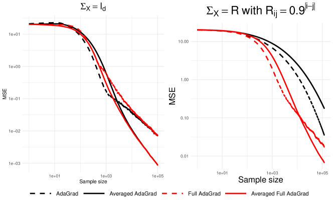
Figure 4: Linear regression case with $(N,d)=(120000,80)$. Mean squared error with respect to the sample size for AdaGrad and Full AdaGrad algorithms with their weighted averaged versions. Two values of $\Sigma_{X}$ are considered: $\Sigma_{X}=I_{d}$ (one the left) and $\Sigma_{X}=R$ (on the right).

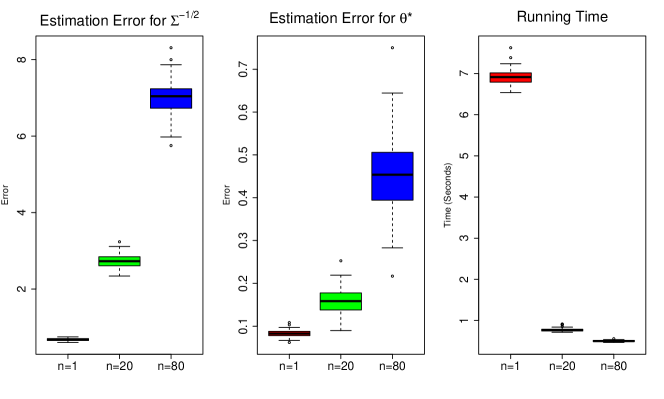
Figure 5: From the left to the right: boxplots of the estimation errors for $\Sigma^{-1/2}$, boxplot of the estimation errors for $\theta$ and boxplots of running time. In each case, $\Sigma_{X}=R$, $(N,d)=(120000,80)$ and three possible values of the streaming batch size are considered: $n=1,20,80$.

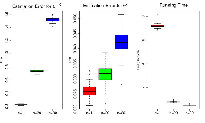
Figure 6: From the left to the right: boxplots of the estimation errors for $\Sigma^{-1/2}$, boxplot of the estimation errors for $\theta$ and boxplots of running time. In each case, $\Sigma_{X}=I_{d}$, $(N,d)=(120000,80)$ and three possible values of the streaming batch size are considered: $n=1,20,80$.

In Figures 5 and 6, we focus on the comparison between the performance of the of the estimates of $\Sigma^{-1/2}$ and $\theta^{*}$ as well as the calculus time obtained with the SWAFA algorithm, with $n=1,20$ and $80$.

We conducted the same experiment with $d=80$ and $N=120000$, considering the logistic model. In Figure 7, we present a comparison of the evolution of the mean squared errors of the estimates obtained with the Adagrad and Full Adagrad algorithms, along with their weighted-averaged versions.

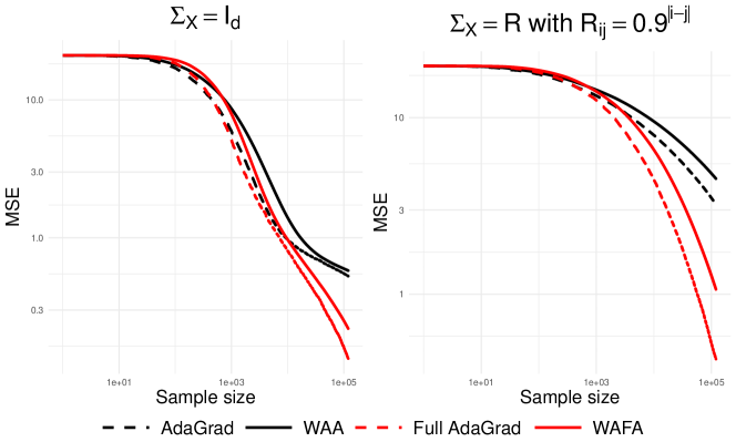
Figure 7: Logstic regression case with $(N,d)=(120000,80)$. Mean squared error with respect to the sample size for AdaGrad and Full AdaGrad algorithms with their weighted averaged versions. Two values of $\Sigma_{X}$ are considered: $\Sigma_{X}=I_{d}$ (one the left) and $\Sigma_{X}=R$ (on the right).

References

• Blackard, (1998) Blackard, J.Β A. (1998). Comparison of neural networks and discriminant analysis in predicting forest cover types. Colorado State University.
• Bottou etΒ al., (2018) Bottou, L., Curtis, F.Β E., and Nocedal, J. (2018). Optimization methods for large-scale machine learning. SIAM review, 60(2):223–311.
• Boyer and Godichon-Baggioni, (2023) Boyer, C. and Godichon-Baggioni, A. (2023). On the asymptotic rate of convergence of stochastic newton algorithms and their weighted averaged versions. Computational Optimization and Applications, 84(3):921–972.
• CΓ©nac etΒ al., (2020) CΓ©nac, P., Godichon-Baggioni, A., and Portier, B. (2020). An efficient averaged stochastic gauss-newton algorithm for estimating parameters of non linear regressions models. arXiv preprint arXiv:2006.12920.
• Dean etΒ al., (2012) Dean, J., Corrado, G., Monga, R., Chen, K., Devin, M., Mao, M., Ranzato, M., Senior, A., Tucker, P., Yang, K., etΒ al. (2012). Large scale distributed deep networks. Advances in neural information processing systems, 25.
• DΓ©fossez etΒ al., (2022) DΓ©fossez, A., Bottou, L., Bach, F., and Usunier, N. (2022). A simple convergence proof of adam and adagrad. Transactions on Machine Learning Research.
• Duchi etΒ al., (2011) Duchi, J., Hazan, E., and Singer, Y. (2011). Adaptive subgradient methods for online learning and stochastic optimization. Journal of machine learning research, 12(7).
• Gadat and Panloup, (2023) Gadat, S. and Panloup, F. (2023). Optimal non-asymptotic analysis of the ruppert–polyak averaging stochastic algorithm. Stochastic Processes and their Applications, 156:312–348.
• Genevay etΒ al., (2016) Genevay, A., Cuturi, M., PeyrΓ©, G., and Bach, F. (2016). Stochastic optimization for large-scale optimal transport. Advances in neural information processing systems, 29.
• Godichon-Baggioni and Lu, (2024) Godichon-Baggioni, A. and Lu, W. (2024). Online stochastic newton methods for estimating the geometric median and applications. Journal of Multivariate Analysis, page 105313.
• Godichon-Baggioni etΒ al., (2024) Godichon-Baggioni, A., Lu, W., and Portier, B. (2024). Online estimation of the inverse of the hessian for stochastic optimization with application to universal stochastic newton algorithms. arXiv preprint arXiv:2401.10923.
• Godichon-Baggioni and Werge, (2023) Godichon-Baggioni, A. and Werge, N. (2023). On adaptive stochastic optimization for streaming data: A newton’s method with o (dn) operations. arXiv preprint arXiv:2311.17753.
• Lazarevic and Obradovic, (2002) Lazarevic, A. and Obradovic, Z. (2002). Boosting algorithms for parallel and distributed learning. Distributed and parallel databases, 11:203–229.
• Mokkadem and Pelletier, (2011) Mokkadem, A. and Pelletier, M. (2011). A generalization of the averaging procedure: The use of two-time-scale algorithms. SIAM Journal on Control and Optimization, 49(4):1523–1543.
• Pelletier, (1998) Pelletier, M. (1998). On the almost sure asymptotic behaviour of stochastic algorithms. Stochastic processes and their applications, 78(2):217–244.
• Pelletier, (2000) Pelletier, M. (2000). Asymptotic almost sure efficiency of averaged stochastic algorithms. SIAM Journal on Control and Optimization, 39(1):49–72.
• Polyak and Juditsky, (1992) Polyak, B.Β T. and Juditsky, A.Β B. (1992). Acceleration of stochastic approximation by averaging. SIAM journal on control and optimization, 30(4):838–855.
• Reagen etΒ al., (2016) Reagen, B., Whatmough, P., Adolf, R., Rama, S., Lee, H., Lee, S.Β K., HernΓ‘ndez-Lobato, J.Β M., Wei, G.-Y., and Brooks, D. (2016). Minerva: Enabling low-power, highly-accurate deep neural network accelerators. ACM SIGARCH Computer Architecture News, 44(3):267–278.
• Robbins and Monro, (1951) Robbins, H. and Monro, S. (1951). A stochastic approximation method. The annals of mathematical statistics, pages 400–407.
• Ruder, (2016) Ruder, S. (2016). An overview of gradient descent optimization algorithms. arXiv preprint arXiv:1609.04747.
• Seide etΒ al., (2014) Seide, F., Fu, H., Droppo, J., Li, G., and Yu, D. (2014). 1-bit stochastic gradient descent and its application to data-parallel distributed training of speech dnns. In Fifteenth annual conference of the international speech communication association.
• Smith, (2017) Smith, L.Β N. (2017). Cyclical learning rates for training neural networks. In 2017 IEEE winter conference on applications of computer vision (WACV), pages 464–472. IEEE.
• Sun etΒ al., (2019) Sun, S., Cao, Z., Zhu, H., and Zhao, J. (2019). A survey of optimization methods from a machine learning perspective. IEEE transactions on cybernetics, 50(8):3668–3681.
• Toulis and Airoldi, (2017) Toulis, P. and Airoldi, E.Β M. (2017). Asymptotic and finite-sample properties of estimators based on stochastic gradients.
• Zhu etΒ al., (2023) Zhu, W., Chen, X., and Wu, W.Β B. (2023). Online covariance matrix estimation in stochastic gradient descent. Journal of the American Statistical Association, 118(541):393–404.